The effect of delay in viral production in within-host models during early infection

ABSTRACT

Delay in viral production may have a significant impact on the early stages of infection. During the eclipse phase, the time from viral entry until active production of viral particles, no viruses are produced. This delay affects the probability that a viral infection becomes established and timing of the peak viral load. Deterministic and stochastic models are formulated with either multiple latent stages or a fixed delay for the eclipse phase. The deterministic model with multiple latent stages approaches in the limit the model with a fixed delay as the number of stages approaches infinity. The deterministic model framework is used to formulate continuous-time Markov chain and stochastic differential equation models. The probability of a minor infection with rapid viral clearance as opposed to a major full-blown infection with a high viral load is estimated from a branching process approximation of the Markov chain model and the results are confirmed through numerical simulations. In addition, parameter values for influenza A are used to numerically estimate the time to peak viral infection and peak viral load for the deterministic and stochastic models. Although the average length of the eclipse phase is the same in each of the models, as the number of latent stages increases, the numerical results show that the time to viral peak and the peak viral load increase.

KEYWORDS:

• Markov chain
• probability of extinction
• stochastic differential equation
• viral infection

MSC CODE:

• 92D30
• 60J28
• 60J70
• 60J85

1. Introduction

The time lag between viral entry into a host cell and active viral production is referred to as the eclipse phase. The duration of this phase is specific to each type of virus. For example, the average length of the eclipse phase for human immunodeficiency virus-1 (HIV-1) infection is around 24 hours and for different strains of influenza virus, the duration of the eclipse phase varies from 4 to 12 hours [14,19,26]. Inclusion of the eclipse phase is important in the study of the early infection of target cells, since the infected host cell may die or be cleared by the immune system prior to active viral production [39].

In this investigation, deterministic and stochastic models are used to study the effect of the eclipse phase on the dynamics of viral establishment and on the peak viral load. Many investigations have focused on the dynamics of HIV and influenza A virus (IAV), applying models with an eclipse phase, e.g. [10,13,14,23,26,32,33,35,39]. A few models have applied stochastic within-host models to study viral infections [18,26,34,42,43,47]. Beauchemin and Handel review the pros and cons of within-host models for influenza infection [13]. In addition, a recent review of within-host models summarizes the many applications to infectious diseases [17].

One of the early deterministic within-host models by Perelson et al. considered the interaction of HIV with CD4+ T cells in  [35]. This model contained an explicit compartment for the eclipse phase. Baccam et al. [10] fitted models with and without an eclipse phase to human influenza patient data and showed that models with an eclipse phase provided a better fit. Similarly, Beauchemin et al. [14] examined treatment effects on IAV applying in vitro data to fit within-host models with and without an eclipse phase and found inclusion of an eclipse phase was also a better fit. Holder and Beauchemin [23] fit influenza A data to a cell culture experiment with high MOI to study average dynamics of a single cell. They found normal and lognormal delays were a better fit to data than either a fixed delay or exponential delay. Anderson and Watson [8] considered the epidemic model with independent gamma-distributed latent and infectious periods and analysed the probability of the major/minor outbreak. Subsequently, many publications analysed models with gamma-distributed periods, e.g. [29–31]. Kakizoe et al. [26] applied several models with different numbers of stages in the eclipse phase to determine the model that best fit data for in vitro experiments with highly pathogenic simian/human immunodeficiency virus (SHIV). The Erlang distribution with three stages in the eclipse phase was the best fit for SHIV. Connections between viral replication and the length of the eclipse phase were discussed in[21], [36].

The delay due to the eclipse phase is the focus of this investigation. We account for different distributions for the delay via a gamma distribution with different shape parameters in a system of ordinary differential equations (ODEs). Inclusion of multiple stages in the eclipse phase allows for different shapes for the distribution of the delay. As the number of stages in the eclipse phase approaches infinity and the mean time to active viral production is held constant, the dynamics of the models with multiple stages approach that of a fixed delay model, a system of delay differential equations (DDEs). We extend this ODE model to include variability in cell/virus numbers to a continuous-time Markov chain (CTMC) and a system of stochastic differential equations (SDEs) and a system of stochastic delay differential equations (SDDEs).

The CTMC model, where the random variables are discrete-valued, accounts for variability in viral establishment due to small cell/virus numbers at the initiation of an infection. The SDE model accounts for variability in timing and in peak viral load after the infection is established. The SDDE is the limiting case of the SDE, where the delay in the eclipse phase has a fixed duration. Although the duration for the eclipse phase in each model has the same mean, it is shown that the time to the peak and the peak viral load increase with the number of stages in the eclipse phase. The mean is insufficient to determine the time to peak viral load or viral peak. Hereafter, we refer to the multiple stages in the eclipse phase as latent stages.

Branching process (BP) approximations of CTMC models have yielded estimates for probability of viral infection in stochastic model formulations [18,33,34,47]. Conway and Coombs [18] were the first to apply BP approximations to an HIV model with an eclipse phase. Noecker et al. [33] applied a within-host model with an eclipse phase to data on SIV. They compared bursting and budding on viral emergence using BPs and other methods to compute the probability of a viral infection. Yan et al. [46] applied BP approximations to a model with multiple latent and infected stages with no cell death except during last stage of the infected cell. Others have used BP with no eclipse stage [34,47]. Stochastic differential equation models of within-host infection have also been constructed to include variability in the infection process during the early stages [42,43,47].

A BP approximation of a CTMC SIR epidemic model was first used by Whittle [45] to compute the probability of a minor or a major epidemic. Here, we use the term ‘minor infection’ to mean that the infection is cleared quickly and the viral load is relatively low so that it may be undetectable, whereas a major infection means the peak viral load is high and the infection has become established. These two types of infection can be distinguished mathematically when ${\mathcal{R}}_0>1$ with a BP approximation, as the BP either hits zero (minor infection) or approaches infinity (major infection). The probability of either a minor or a major infection can be computed as a function of the initial number of virions and the initial number of infected cells in each stage. As expected the BP estimates show that a minor infection (rapid viral clearance) has a greater probability of occurrence when the initial viral load is small with no or few latent and infected cells and the greater the number of infected cells the more likely that there will be a major infection.

Numerical examples illustrating the infection dynamics by the various deterministic and stochastic modelling approaches are investigated in the context of IAV infection. Influenza A virus targets the epithelial cells of the upper respiratory tract with an incubation period of about 48 hours and a range of 24–96 hours [13]. Beauchemin and Handel [13] report the lifespan of an infected cell from 12 to 48 hours, the average lifespan of a virion from 0.5 to 3 hours and the length of eclipse phase from 3 to 12 hours. We apply the in vitro experimental data for IAV estimated by Beauchemin et al. [14] for the model with one stage during the eclipse phase (the eclipse model) and the model with a fixed delay (the delay model). We rescale the parameter values to satisfy our model assumptions (see details in Section 5), and numerical experiments are performed to compare model outcomes.

In the following Section 2, the deterministic within-host model is introduced with a single latent stage. This deterministic model is extended to one with multiple latent stages and with a fixed delay. The basic reproduction number ${\mathcal{R}}_0$ is calculated for each model. In Section 3, a continuous-time Markov chain model for multiple latent stages is formulated. Applying theory from BP, expressions for the probabilities of a minor infection are derived near the infection-free equilibrium, with constant number of uninfected cells, during the early stages of infection. In Section 4, a stochastic differential equation model for multiple latent stages and a stochastic delay differential equation model are formulated. In Section 5, several numerical simulations show the parameter sensitivity of the BP estimate for probability of a minor infection for IAV. In addition, the variability in the dynamics at specific time points and at the time to peak viral infection are compared in the ordinary and stochastic differential equation models. We conclude by summarizing the results of this modelling study and discuss some implications for early therapeutic intervention and some ways to extend to this study.

2. Deterministic models

We first introduce the basic deterministic model with one latent stage. Then we extend this model, allowing time for the virus to replicate inside the cell. The second model assumes n latent stages for the eclipse phase, $L_1,\dots ,L_n$, each with transition rate ${\delta }_k$, $k=1,\dots ,n$ and the third model assumes a fixed delay of length $1/\delta$. One important assumption is that the infection rate of the target cells by one virion is accompanied by a loss of one virion. In particular, one virion results in infection of a target cell. We focus on the case ${\delta }_k=n\delta$. In the particular case when there is no death during any of the latent stages, the average time of the eclipse phase is equal to $1/\delta$ for all three models, for either one or n latent stages or for a fixed delay.

2.1. Basic model with one latent stage

A simple model for viral infection of target cells includes variables for the density of uninfected target cells, H, eclipse-phase cells, L, infected cells, I, and the concentration of virions V or free viruses, outside the cells. The model has the form: (1) $\mathrm{TargetCells}\left\{\begin{array}{ll}\frac{\mathrm{d}H}{\mathrm{d}t}& =\mathrm{\Lambda }-\beta VH-{\mu }_{H}H\\ \frac{\mathrm{d}L}{\mathrm{d}t}& =\beta VH-\delta L-\mu L\\ \frac{\mathrm{d}I}{\mathrm{d}t}& =\delta L-{\mu }_{I}I,\end{array}\right.$(1) (2) $\mathrm{Virions}\left\{\begin{array}{ll}\frac{\mathrm{d}V}{\mathrm{d}t}& =bI-\beta VH-cV,\end{array}\right.$(2) where β is the transmission rate of the virus, δ is the rate an eclipse-phase cell becomes an infected cell, b is the viral production rate, c is the clearance rate of the virus, and ${\mu }_H$, μ, and ${\mu }_I$ are the death rates of H, L, and I, respectively. An eclipse-phase cell and an infected cell may have a shorter lifespan (larger death rates) than a healthy cell: ${\mu }_H\le \mu \le {\mu }_I.$ The transmission term $\beta VH$ also appears in the equation for virions because of the assumption that it takes only one virion to infect a target cell. The possibility of multiply-infected cells is excluded. The total number of cells that have not died is $N\left(t\right)=H\left(t\right)+L\left(t\right)+I\left(t\right),$ where $\frac{\mathrm{d}N}{\mathrm{d}t}=\mathrm{\Lambda }-{\mu }_{H}H-\mu L-{\mu }_{I}I.$ The infection-free equilibrium is L=I=V =0 and $\overline{H}=\mathrm{\Lambda }/{\mu }_H$. For in vitro experiments, it is often the case that $\mathrm{\Lambda }=0$ and ${\mu }_H=0$. For this case, $\overline{H}=H\left(0\right)$. For simplicity, we refer to model (1(1) $\mathrm{TargetCells}\left\{\begin{array}{ll}\frac{\mathrm{d}H}{\mathrm{d}t}& =\mathrm{\Lambda }-\beta VH-{\mu }_{H}H\\ \frac{\mathrm{d}L}{\mathrm{d}t}& =\beta VH-\delta L-\mu L\\ \frac{\mathrm{d}I}{\mathrm{d}t}& =\delta L-{\mu }_{I}I,\end{array}\right.$(1) )–(2(2) $\mathrm{Virions}\left\{\begin{array}{ll}\frac{\mathrm{d}V}{\mathrm{d}t}& =bI-\beta VH-cV,\end{array}\right.$(2) ) as the HLIV model.

The basic reproduction number for the HLIV models (1(1) $\mathrm{TargetCells}\left\{\begin{array}{ll}\frac{\mathrm{d}H}{\mathrm{d}t}& =\mathrm{\Lambda }-\beta VH-{\mu }_{H}H\\ \frac{\mathrm{d}L}{\mathrm{d}t}& =\beta VH-\delta L-\mu L\\ \frac{\mathrm{d}I}{\mathrm{d}t}& =\delta L-{\mu }_{I}I,\end{array}\right.$(1) )–(2(2) $\mathrm{Virions}\left\{\begin{array}{ll}\frac{\mathrm{d}V}{\mathrm{d}t}& =bI-\beta VH-cV,\end{array}\right.$(2) ) can be computed from the next generation matrix approach at the infection-free equilibrium as in [38,44]: (3) ${\mathcal{R}}_0^{\left(1\right)}=\frac{b\beta \overline{H}\delta }{{\mu }_I(\beta \overline{H}+c)(\delta +\mu )},$(3) where the superscript $\left(1\right)$ refers to one latent stage. The basic reproduction number can also be computed by counting the number of secondary cases arising from one infected cell. Each infected cell produces $b/{\mu }_I$ virions during its lifetime. Each virion produces $\beta \overline{H}/(\beta \overline{H}+c)$ eclipse-phase cells during its lifetime and the fraction $\delta /(\delta +\mu )$ that survives become infected cells. A similar interpretation applies to production of virions. The infection-free equilibrium $\overline{H}$ is locally asymptotically stable if ${\mathcal{R}}_0^{\left(1\right)}<1$ [44]. If $\delta \to \mathrm{\infty }$, then the model with no latent stage has a basic reproduction number given by (4) ${\mathcal{R}}_0^{\left(0\right)}=\frac{b\beta \overline{H}}{{\mu }_I(\beta \overline{H}+c)}.$(4)

2.2. Multiple latent stage model

The model with a single latent stage L is extended to one with n stages (Figure 1). The length of each stage is shortened and has a distinct transition rate ${\delta }_k$ ($k=1,\dots ,n$). In the case that there are no deaths during each latent stage, the total mean duration of the eclipse phase is $1/\delta =\sum _{k=1}^{n}1/{\delta }_k$. The advantage of increasing the number of the latent stages is to ensure viral reproduction does not occur immediately after a virus enters a cell. Lloyd showed that including n infectious stages corresponds to an underlying gamma-distributed infectious period [29,30]. The sum of n independent exponential distributions with parameter $1/\left(n\delta \right)$ is an Erlang distribution, a special case of the gamma distribution, with shape parameter n and rate parameter $n\delta$. Figure 2 displays the Erlang probability density function (pdf) for n=1,2,3,4,5 latent stages as well as for the limiting case when $n\to \mathrm{\infty }$, a fixed delay, with a dirac delta function with probability mass concentrated at $1/\delta$.

Figure 1. Compartmental diagram of the model with multiple latent stages. The circles represent compartments H, $L_1$, $\dots$, $L_n$, I, (right to left), virions V . The terms ${\mu }_H$, ${\mu }_k$ $(k=1,\dots ,n)$, and ${\mu }_I$ are death rates associated with the particular state H, $L_k$ $(k=1,\dots ,n)$, and I, respectively. Parameter Λ is the birth rate of cells, b is the viral production rate of virions from an actively producing cell and c is the clearance rate of virus. Parameter ${\delta }_k$ $(k=1,\dots ,n)$ is the transition rate between latent stages and the transition rate into stage I. Parameter β is the rate that virions V infect a cell H.

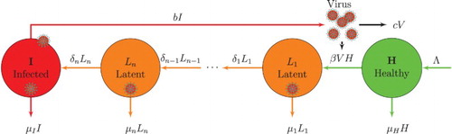
Figure 2. The probability density function (pdf) corresponding to an Erlang distribution is graphed with shape parameter $\ell =n$ and rate parameter $\lambda =n\delta$ for $\delta =0.31$ (see Table 2 for IAV infection) [14]. The pdf has the form $f\left(t\right)={\lambda }^{\ell }{t}^{\ell -1}\exp (-\lambda t)/(\ell -1)!$. The mean of the pdf is $1/\delta$. The fixed delay model has a generalized pdf, with a fixed duration of $1/\delta$, i.e. a dirac delta function with probability mass concentrated at $1/\delta$.

The differential equations for target cells H and virions V are the same as in the original HLIV models (1(1) $\mathrm{TargetCells}\left\{\begin{array}{ll}\frac{\mathrm{d}H}{\mathrm{d}t}& =\mathrm{\Lambda }-\beta VH-{\mu }_{H}H\\ \frac{\mathrm{d}L}{\mathrm{d}t}& =\beta VH-\delta L-\mu L\\ \frac{\mathrm{d}I}{\mathrm{d}t}& =\delta L-{\mu }_{I}I,\end{array}\right.$(1) )–(2(2) $\mathrm{Virions}\left\{\begin{array}{ll}\frac{\mathrm{d}V}{\mathrm{d}t}& =bI-\beta VH-cV,\end{array}\right.$(2) ). However, there are n latent stages that make up the eclipse phase. See Figure 1. The differential equations for n latent stages and one infected stage are given below: (5) $\begin{array}{rl}\frac{\mathrm{d}{L}_1}{\mathrm{d}t}& =\beta VH-{\delta }_1{L}_1-{\mu }_1{L}_1\\ \frac{\mathrm{d}{L}_k}{\mathrm{d}t}& ={\delta }_{k-1}{L}_{k-1}-{\delta }_k{L}_k-{\mu }_k{L}_k,\mathrm{for}k=2,3,\dots ,n,\\ \frac{\mathrm{d}I}{\mathrm{d}t}& ={\delta }_n{L}_n-{\mu }_{I}I.\end{array}$(5) The generalization from one stage to n stages yields the following basic reproduction number: ${\hat{\mathcal{R}}}_0^{\left(n\right)}=\frac{b\beta \overline{H}}{{\mu }_I(\beta \overline{H}+c)}\prod _{k=1}^n\left(\frac{{\delta }_k}{{\delta }_k+{\mu }_k}\right)={\mathcal{R}}_0^{\left(0\right)}\prod _{k=1}^n\left(\frac{{\delta }_k}{{\delta }_k+{\mu }_k}\right),$ where ${\mathcal{R}}_0^{\left(0\right)}$ is defined in (4(4) ${\mathcal{R}}_0^{\left(0\right)}=\frac{b\beta \overline{H}}{{\mu }_I(\beta \overline{H}+c)}.$(4) ). If there is no cell death during the eclipse phase, ${\mu }_k=0$, then ${\mathcal{R}}_0^n={\mathcal{R}}_0^{\left(0\right)}$. Local stability of $\overline{H}$ follows if ${\hat{\mathcal{R}}}_0^{\left(n\right)}<1$ [44]. The following analysis is restricted to the case with ${\delta }_k=n\delta$ and death rates ${\mu }_k=\mu \ge 0$. The basic reproduction number in this case has the form: (6) ${\mathcal{R}}_0^{\left(n\right)}=\frac{b\beta \overline{H}}{{\mu }_I(\beta \overline{H}+c)}{\left(\frac{n\delta }{n\delta +\mu }\right)}^n={\mathcal{R}}_0^{\left(0\right)}{\left(\frac{n\delta }{n\delta +\mu }\right)}^n.$(6)

2.3. Fixed delay model

Next, we extend the original HLIV model (1(1) $\mathrm{TargetCells}\left\{\begin{array}{ll}\frac{\mathrm{d}H}{\mathrm{d}t}& =\mathrm{\Lambda }-\beta VH-{\mu }_{H}H\\ \frac{\mathrm{d}L}{\mathrm{d}t}& =\beta VH-\delta L-\mu L\\ \frac{\mathrm{d}I}{\mathrm{d}t}& =\delta L-{\mu }_{I}I,\end{array}\right.$(1) )–(2(2) $\mathrm{Virions}\left\{\begin{array}{ll}\frac{\mathrm{d}V}{\mathrm{d}t}& =bI-\beta VH-cV,\end{array}\right.$(2) ) to one with a fixed delay τ. The differential equations for the latent and infected cell densities are given below: (7) $\begin{array}{rl}\frac{\mathrm{d}L\left(t\right)}{\mathrm{d}t}& =\beta V\left(t\right)H\left(t\right)-\beta V(t-\tau )H(t-\tau ){\mathrm{e}}^{-\mu \tau }-\mu L\left(t\right)\\ \frac{\mathrm{d}I\left(t\right)}{\mathrm{d}t}& =\beta V(t-\tau )H(t-\tau ){\mathrm{e}}^{-\mu \tau }-{\mu }_{I}I\left(t\right),\end{array}$(7) where the proportion of eclipse-phase cells that survives to become infected is ${\mathrm{e}}^{-\mu \tau }={\mathrm{e}}^{-\mu /\delta }$. Since the delay until viral reproduction is fixed at τ, the duration of the latent stage is exactly τ, e.g. the associated generalized pdf for the duration of the latent stage is a dirac delta function with probability mass concentrated at $1/\delta$ (Figure 2).

The basic reproduction number for the delay model is (8) ${\mathcal{R}}_0^{\left(d\right)}=\frac{b\beta \overline{H}{\mathrm{e}}^{-\mu /\delta }}{{\mu }_I(\beta \overline{H}+c)}={\mathcal{R}}_0^{\left(0\right)}{\mathrm{e}}^{-\mu /\delta }.$(8) As $n\to \mathrm{\infty }$, the basic reproduction number, given in (6(6) ${\mathcal{R}}_0^{\left(n\right)}=\frac{b\beta \overline{H}}{{\mu }_I(\beta \overline{H}+c)}{\left(\frac{n\delta }{n\delta +\mu }\right)}^n={\mathcal{R}}_0^{\left(0\right)}{\left(\frac{n\delta }{n\delta +\mu }\right)}^n.$(6) ), for n latent stages ${\mathcal{R}}_0^{\left(n\right)}$, approaches ${\mathcal{R}}_0^{\left(d\right)}$, since $\underset{n\to \mathrm{\infty }}{lim}{\left(\frac{n\delta }{n\delta +\mu }\right)}^n={\mathrm{e}}^{-\mu /\delta }.$ Local stability of $\overline{H}$ follows if ${\mathcal{R}}_0^{\left(d\right)}<1$ (verified in Appendix A.1).

3. Continuous-time Markov chain

A stochastic model with discrete events but continuous in time is formulated based on the assumed rates in the within-host model with multiple latent stages. This model is particularly useful in computing the probability of establishment of a viral infection given that target cells are exposed to virions, eclipse-phase cells or infected target cells. It is important to note that we are assuming a homogeneously mixed population of virions and cells.

3.1. Multiple latent stages

The infinitesimal transition rates of a continuous-time Markov chain (CTMC) are described in Table 1. Each random variable is discrete-valued, taking values in $\{0,1,2\dots \}$, where H, $L_i$, and I are bounded above by $\overline{H}$. For example, let $\left(\mathrm{\Delta }H\right(t),\mathrm{\Delta }{L}_1(t),I(t),\mathrm{\Delta }V(t\left)\right)=\left(H\right(t+\mathrm{\Delta }t)-H(t),L_1(t+\mathrm{\Delta }t)-L_1(t),I(t+\mathrm{\Delta }t)-I(t),V(t+\mathrm{\Delta }t)-V(t\left)\right)$. The single event, infection of a target cell has probability $\begin{array}{rl}\mathbb{P}\left\{\right(\mathrm{\Delta }H\left(t\right),\mathrm{\Delta }{L}_1\left(t\right),\mathrm{\Delta }I\left(t\right),\mathrm{\Delta }V\left(t\right))& =(-1,1,0,-1)|\left(H\right(t),L_i(t),I(t),V(t\left)\right)\}\\ & =\beta V\left(t\right)H\left(t\right)\mathrm{\Delta }t+o\left(\mathrm{\Delta }t\right).\end{array}$ (See e.g. [2,27] .) Note the dependence on the current state at time t. The other transition rates are defined in Table 1, where, for simplicity, the time dependence is omitted, i.e. $H\equiv H\left(t\right)$, $L_1\equiv L_1\left(t\right)$, etc. The underlying assumption in a CTMC is that the interevent time is exponentially distributed with parameter λ, where λ is the sum of the rates in Table 1: $\lambda =\mathrm{\Lambda }+{\mu }_{H}H+\beta VH+(n\delta +\mu )\sum _{k=1}^n{L}_k+{\mu }_{I}I+cV+bI.$

Table 1. Infinitesimal transition rates for the multiple latent stage model.

Event	Description	Change	Probability
1	Birth of H	$H\to H+1$	$\mathrm{\Lambda \Delta }t+o\left(\mathrm{\Delta }t\right)$
2	Infection of H	$(H,L_1,V)\to (H-1,L_1+1,V-1)$	$\beta VH\mathrm{\Delta }t+o\left(\mathrm{\Delta }t\right)$
3	Death of H	$H\to H-1$	${\mu }_{H}H\mathrm{\Delta }t+o\left(\mathrm{\Delta }t\right)$
4	Death of I	$I\to I-1$	${\mu }_{I}I\mathrm{\Delta }t+o\left(\mathrm{\Delta }t\right)$
5	Viral Production of V	$V\to V+1$	$bI\mathrm{\Delta }t+o\left(\mathrm{\Delta }t\right)$
6	Death of V	$V\to V-1$	$cV\mathrm{\Delta }t+o\left(\mathrm{\Delta }t\right)$
$6+k^{\mathrm{a}}$	Transition of $L_k$ to$L_{k+1}$	$(L_k,L_{k+1})\to (L_k-1,L_{k+1}+1)$	$n\delta L_k\mathrm{\Delta }t+o\left(\mathrm{\Delta }t\right)$
6+n	Transition of $L_n$ to I	$(L_n,I)\to (L_n-1,I+1)$	$n\delta L_n\mathrm{\Delta }t+o\left(\mathrm{\Delta }t\right)$
$6+(n+k{)}^{\mathrm{b}}$	Death of $L_k$	$L_k\to L_k-1$	$\mu L_k\mathrm{\Delta }t+o\left(\mathrm{\Delta }t\right)$

${}^{\mathrm{a}}$ $k=1,\dots ,n-1$ ,${}^{\mathrm{b}}$ $k=1,\dots ,n$.

Table 2. Parameter values for IAV taken from  [14] for the HLIV models (1(1) $\mathrm{TargetCells}\left\{\begin{array}{ll}\frac{\mathrm{d}H}{\mathrm{d}t}& =\mathrm{\Lambda }-\beta VH-{\mu }_{H}H\\ \frac{\mathrm{d}L}{\mathrm{d}t}& =\beta VH-\delta L-\mu L\\ \frac{\mathrm{d}I}{\mathrm{d}t}& =\delta L-{\mu }_{I}I,\end{array}\right.$(1) )–(2(2) $\mathrm{Virions}\left\{\begin{array}{ll}\frac{\mathrm{d}V}{\mathrm{d}t}& =bI-\beta VH-cV,\end{array}\right.$(2) ).

Parameter	Value
β	$6.21\times {10}^{-8}$ h^−1
δ (τ)	0.31 h^−1 (3.2 h)
${\mu }_I$	0.076 h^−1
b	3.48 h^−1
c	0.105 h^−1
$\overline{H}$	$6.7\times {10}^6$ cells

3.2. Branching process approximation

The CTMC model is approximated near the infection-free equilibrium, when $H=\overline{H}$ is constant. The infinitesimal transition rates in Table 1 become linear in the variables $L_k$, I and V for small intervals of time $\mathrm{\Delta }t$ when $H=\overline{H}$ is constant. Therefore, we can apply a BP approximation and utilize probability generating functions (pgfs) to define the dynamics the probability of generating a new virion, a new cell or a transition, when initiated by one virion, one eclipse-phase cell or one infected cell [3,5,6,9].

It is well-known from BP theory that the fixed point of the pgfs yield an asymptotic approximation (as $t\to \mathrm{\infty }$) of the probability of ultimate extinction [9,22].The BP estimates come from a multitype birth and death linear approximation of the Markov chain model near the infection-free state (either states hit zero or approach infinity in the limit) [5,6,9]. As a linear approximation near the infection-free state, when $H=\overline{H}$ is constant, the BP approximation is reasonable during the early stages of infection, provided there is exponential growth of $L_k$, I, or V of sufficient magnitude. Only the eclipse-phase cells $L_k$, $k=1,\dots ,n$, infected cells I, and virions V are considered as $H=\overline{H}$ is constant.

A pgf corresponding to each n+2 variables, the eclipse-phase cells, $L_k$, infected cells, I, and virions V, represents the number of ‘offspring’ of type $L_k$, I or V generated from one cell or one virion. The domain of each pgf is the set $u\in [0,1{]}^{n+2}$, where $u=(u_1,\dots ,u_{n+2})$. The pgf $f_1\left(u\right)$ is the pgf for latent cell population $L_1$ given $L_1\left(0\right)=1$ and $L_k\left(0\right)=I\left(0\right)=V\left(0\right)=0$, $k=2,\dots ,n$ and $f_{n+2}\left(u\right)$ is the pgf for the virions, given $L_k\left(0\right)=I\left(0\right)=0$, $k=1,\dots ,n$ and $V\left(0\right)=1$. The pgfs for the n+2 states are defined below: $\begin{array}{rl}{f}_k\left(u\right)& =\frac{n\delta u_{k+1}+\mu }{n\delta +\mu },\mathrm{for}k=1,2,\dots ,n,\\ f_{n+1}\left(u\right)& =\frac{b{u}_{n+1}{u}_{n+2}+{\mu }_I}{b+{\mu }_I},\\ f_{n+2}\left(u\right)& =\frac{\beta \overline{H}{u}_1+c}{\beta \overline{H}+c}.\end{array}$ For example, in $f_k\left(u\right)$, the term $n\delta /(n\delta +\mu )$ is the probability one latent cell in stage k transitions to the next latent stage k+1 for $k=1,2,\dots ,n-1$ (or transition to the infected stage if k=n), and $\mu /(n\delta +\mu )$ is the probability that a latent cell dies before transition to the next stage. In $f_{n+1}\left(u\right)$, the term $b/(b+{\mu }_I)$ is the probability one infected cell produces one virion. The probabilities follow from the fact that time is continuous, changes occur during a small period of time $\mathrm{\Delta }t$, and the assumptions in Table 1 [5,6].

From BP theory, it follows that the fixed point of the system $q_i=f_i(q_1,q_2,\dots ,q_{n+2})$ for $i=1,2\dots ,n+2$ is the probability of ultimate extinction [3,4,9,22]. A detailed derivation for the BP approximation can be found in [24]. Given $I\left(0\right)=1$ and $L_k\left(0\right)=V\left(0\right)=0$, the probability of extinction is $q_{n+1}$. The latter two probabilities, $q_{n+1}$ and $q_{n+2}$, are associated with infected cells and virions, respectively. For our model, there exists a unique fixed point that lies in the interior of the set $(0,1{)}^{n+2}$, provided ${\mathcal{R}}_0^{\left(n\right)}>1$ [6]. An analytical expression for this fixed point can be computed as follows: (9) $\begin{array}{rl}{q}_k& ={\left(\frac{n\delta }{n\delta +\mu }\right)}^{n-k+1}\frac{1}{{\mathcal{R}}_0^{\left(n\right)}}+\frac{\mu }{n\delta +\mu }\sum _{l=0}^{n-k}{\left(\frac{n\delta }{n\delta +\mu }\right)}^l,\mathrm{for}k=1,2,\dots ,n,\\ q_{n+1}& =\frac{1}{{\mathcal{R}}_0^{\left(n\right)}},\\ q_{n+2}& =q_1\frac{\beta \overline{H}}{\beta \overline{H}+c}+\frac{c}{\beta \overline{H}+c}.\end{array}$(9) If ${\mathcal{R}}_0^{\left(n\right)}<1$, the unique fixed point is $q_i=1$ for $i=1,\dots ,n+2$. The formulas in the case of n=1, one latent stage, agree with the expressions computed in [33]. The probabilities of ultimate extinction correspond to the probabilities of a minor infection in the CTMC model. If there is no cell death during the eclipse phase, $\mu =0$, then $q_k=1/{\mathcal{R}}^{\left(0\right)}$ for $k=1,\dots ,n+1$ [46]. With cell death in the eclipse phase, $\mu >0$, the probability of a minor infection or rapid clearance of the infection is increased.

Each term in the expressions for $q_k$, $q_{n+1}$, and $q_{n+2}$ has a biological interpretation. For example, the term $\left[n\delta /\right(n\delta +\mu ){]}^l$ is the probability of a transition between l latent stages, $\mu /(n\delta +\mu )$ is the probability of a death in a latent stage, and $1/{\mathcal{R}}_0^{\left(n\right)}$ is the probability of an unsuccessful infection at the infected stage. Probability of a minor infection for one virion is defined by the two terms in $q_{n+2}$. Either the virus enters a cell (first latent stage $L_1$) and there is a minor infection with probability $q_1\beta \overline{H}/(\beta \overline{H}+c)$ or the virion is cleared with probability $c/(\beta \overline{H}+c)$. Similar interpretations can be applied to the terms in $q_k$, for a cell in the kth latent stage, where there are either transitions between stages but an unsuccessful infection or a death in one of the latent stages prior to reaching the infected stage.

Near the infection-free state, an underlying assumption in the BP approximation is that the cells and virions are independent of other states. Therefore, for small initial values, $L_k\left(0\right)=l_{k_0},$ $I\left(0\right)=i_0$ and $V\left(0\right)=v_0$ for $l_{k_0},i_0,v_0\in \{0,1,\dots \}$, the BP approximation yields the probability of a minor infection as (10) $\left(\prod _{k=1}^n{q}_k^{l_{k_0}}\right)q_{n+1}^{i_0}{q}_{n+2}^{v_0}.$(10) Alternately, the probability of a major infection is (11) $1-\left(\prod _{k=1}^n{q}_k^{l_{k_0}}\right)q_{n+1}^{i_0}{q}_{n+2}^{v_0}.$(11) As the fixed delay model is the limiting case of the model with n latent stages, we compute the average probability of a minor infection for the n latent classes given in (9(9) $\begin{array}{rl}{q}_k& ={\left(\frac{n\delta }{n\delta +\mu }\right)}^{n-k+1}\frac{1}{{\mathcal{R}}_0^{\left(n\right)}}+\frac{\mu }{n\delta +\mu }\sum _{l=0}^{n-k}{\left(\frac{n\delta }{n\delta +\mu }\right)}^l,\mathrm{for}k=1,2,\dots ,n,\\ q_{n+1}& =\frac{1}{{\mathcal{R}}_0^{\left(n\right)}},\\ q_{n+2}& =q_1\frac{\beta \overline{H}}{\beta \overline{H}+c}+\frac{c}{\beta \overline{H}+c}.\end{array}$(9) ) and then let $n\to \mathrm{\infty }$, i.e. $q_L=\underset{n\to \mathrm{\infty }}{lim}\frac{\sum _{k=1}^n{q}_k}{n}.$ For the infected cells I and virions V, we compute the limiting value of $q_{n+1}$ and $q_{n+2}$ given in (9(9) $\begin{array}{rl}{q}_k& ={\left(\frac{n\delta }{n\delta +\mu }\right)}^{n-k+1}\frac{1}{{\mathcal{R}}_0^{\left(n\right)}}+\frac{\mu }{n\delta +\mu }\sum _{l=0}^{n-k}{\left(\frac{n\delta }{n\delta +\mu }\right)}^l,\mathrm{for}k=1,2,\dots ,n,\\ q_{n+1}& =\frac{1}{{\mathcal{R}}_0^{\left(n\right)}},\\ q_{n+2}& =q_1\frac{\beta \overline{H}}{\beta \overline{H}+c}+\frac{c}{\beta \overline{H}+c}.\end{array}$(9) ): $q_I=\underset{n\to \mathrm{\infty }}{lim}{q}_{n+1}\mathrm{and}{q}_V=\underset{n\to \mathrm{\infty }}{lim}{q}_{n+2}.$ The limiting values (derived in the Appendix A.2) are (12) $\begin{array}{rl}{q}_L& =1-\frac{\delta }{\mu }\left(1-{\mathrm{e}}^{-\mu /\delta }\right)\left(1-\frac{1}{{\mathcal{R}}_0^{\left(d\right)}}\right)\\ q_I& =\frac{1}{{\mathcal{R}}_0^{\left(d\right)}}\\ q_V& =\frac{{\mu }_I}{b}+\frac{\beta \overline{H}(1-{\mathrm{e}}^{-\mu /\delta })+c}{\beta \overline{H}+c}.\end{array}$(12) These probabilities provide an estimate for a minor infection in a stochastic fixed delay model.

For ${\mathcal{R}}_0^{\left(n\right)}>1$ and ${\mathcal{R}}_0^{\left(d\right)}>1$, it is straightforward to verify that the expressions in (9(9) $\begin{array}{rl}{q}_k& ={\left(\frac{n\delta }{n\delta +\mu }\right)}^{n-k+1}\frac{1}{{\mathcal{R}}_0^{\left(n\right)}}+\frac{\mu }{n\delta +\mu }\sum _{l=0}^{n-k}{\left(\frac{n\delta }{n\delta +\mu }\right)}^l,\mathrm{for}k=1,2,\dots ,n,\\ q_{n+1}& =\frac{1}{{\mathcal{R}}_0^{\left(n\right)}},\\ q_{n+2}& =q_1\frac{\beta \overline{H}}{\beta \overline{H}+c}+\frac{c}{\beta \overline{H}+c}.\end{array}$(9) ) satisfy $q_{n+2}>q_1\ge q_2\ge \cdots \ge q_n\ge q_{n+1}$ and those in (12(12) $\begin{array}{rl}{q}_L& =1-\frac{\delta }{\mu }\left(1-{\mathrm{e}}^{-\mu /\delta }\right)\left(1-\frac{1}{{\mathcal{R}}_0^{\left(d\right)}}\right)\\ q_I& =\frac{1}{{\mathcal{R}}_0^{\left(d\right)}}\\ q_V& =\frac{{\mu }_I}{b}+\frac{\beta \overline{H}(1-{\mathrm{e}}^{-\mu /\delta })+c}{\beta \overline{H}+c}.\end{array}$(12) ) satisfy $q_V>q_L\ge q_I.$ With no cell deaths in the eclipse phase, then $q_k=1/{\mathcal{R}}^{\left(0\right)}$, $k=1,\dots ,n+1$, and $q_L=1/{\mathcal{R}}^{\left(0\right)}=q_I$. An obvious conclusion, shown by the expressions in (11(11) $1-\left(\prod _{k=1}^n{q}_k^{l_{k_0}}\right)q_{n+1}^{i_0}{q}_{n+2}^{v_0}.$(11) ), is that there is a greater probability of a major infection the further the infection has progressed, when there are greater numbers of eclipse phase and infected cells. If the virus is cleared rapidly so that $v_0=0$ and only a few cells are in the eclipse phase, the infection may still have a high probability of being cleared (minor infection) if there is cell death during these stages, $\mu >0$, such as through drug treatment that eliminates virions (increases c) or eclipse-phase and infected cells (increases μ and ${\mu }_I$) or prevents viral production (decreases b).

4. Stochastic differential equations

To account for variability in number of cells and virions after the virus becomes established, we consider another stochastic formulation. In this case, when numbers of cells and virions are large, the state variables and time are represented by continuous random variables, e.g. $H\left(t\right)\in [0,\overline{H}]$. We formulate a system of stochastic differential equations (SDEs) for the multiple latent stage model and stochastic delay differential equations (SDDEs) for the fixed delay model.

4.1. Multiple latent stages

A system of Itô SDEs is derived of the form $\mathrm{d}\overrightarrow{X}\left(t\right)=f\left(\overrightarrow{X}\right(t\left)\right)\mathrm{d}t+\mathrm{\Sigma }\left(\overrightarrow{X}\right(t\left)\right)\mathrm{d}\overrightarrow{W}\left(t\right),$ where $f\left(\overrightarrow{X}\right(t\left)\right)$ is the drift vector, $\mathrm{\Sigma }\left(\overrightarrow{X}\right(t\left)\right)$ is the diffusion matrix, and $\overrightarrow{W}\left(t\right)$ is a vector of independent Wiener processes. To formulate the SDEs, the transition rates from Table 1 are used to compute the expectation and covariance in the processes to order $\mathrm{\Delta }t$ [1,7]. The drift vector $f\left(\overrightarrow{X}\right(t\left)\right)\approx \mathbb{E}\left(\mathrm{\Delta }\overrightarrow{X}\right(t\left)\right)$ to order $\mathrm{\Delta }t$ is $f\left(\overrightarrow{X}\right(t\left)\right)\approx \left[\begin{array}{c}\mathrm{\Lambda }-\beta VH-{\mu }_{H}H\\ \beta VH-n\delta L_1-\mu L_1\\ ⋮\\ n\delta (L_{k-1}-L_k)-\mu L_k\\ ⋮\\ n\delta L_n-{\mu }_{I}I\\ bI-\beta VH-cV\end{array}\right].$ Also with the aid of Table 1, the covariance matrix $G\left(X\right(t\left)\right)\approx \mathbb{E}\left(\mathrm{\Delta }\overrightarrow{X}\right(t\left)\right(\mathrm{\Delta }\overrightarrow{X}\left(t\right){)}^{\mathrm{T}})$ to order $\mathrm{\Delta }t$ can be used to compute the diffusion matrix $\mathrm{\Sigma }\left(\overrightarrow{X}\right(t\left)\right)$, where $\mathrm{\Sigma }{\mathrm{\Sigma }}^{\mathrm{T}}=G$ [1,7]. The multiple latent stage model takes the form of the following Itô SDE: $\begin{array}{rl}\mathrm{d}H& =(\mathrm{\Lambda }-\beta VH-{\mu }_{H}H)\mathrm{d}t+\sqrt{\mathrm{\Lambda }}\mathrm{d}{W}_1-\sqrt{\beta VH}\mathrm{d}{W}_2-\sqrt{{\mu }_{H}H}\mathrm{d}{W}_3,\\ \mathrm{d}{L}_1& =(\beta VH-n\delta L_1-\mu L_1)\mathrm{d}t+\sqrt{\beta VH}\mathrm{d}{W}_2-\sqrt{n\delta L_1}\mathrm{d}{W}_7-\sqrt{\mu L_1}\mathrm{d}{W}_{6+(n+1)},\\ \mathrm{d}{L}_k& =\left(n\delta \right(L_{k-1}-L_k)-\mu L_k)\mathrm{d}t\\ & -\sqrt{n\delta L_k}\mathrm{d}{W}_{6+k}+\sqrt{n\delta L_{k-1}}\mathrm{d}{W}_{6+(k-1)}-\sqrt{\mu L_k}\mathrm{d}{W}_{6+(n+k)},\mathrm{for}k=2,3\dots ,n\\ \mathrm{d}I& =(n\delta L_n-{\mu }_{I}I)\mathrm{d}t-\sqrt{{\mu }_{I}I}\mathrm{d}{W}_4+\sqrt{n\delta L_n}\mathrm{d}{W}_{6+n},\\ \mathrm{d}V& =(bI-\beta VH-cV)\mathrm{d}t-\sqrt{\beta VH}\mathrm{d}{W}_2+\sqrt{bI}\mathrm{d}{W}_5-\sqrt{cV}\mathrm{d}{W}_6,\end{array}$ where $W_k\equiv W_k\left(t\right)$ for $k=1,2,\dots ,6+2n$ are 6+2n independent Wiener processes. The time-dependence is omitted for simplicity, $H\equiv H\left(t\right)$, $L_1\equiv L_1\left(t\right)$, etc.

4.2. Stochastic delay differential equation

We formulate the stochastic delay differential equation (SDDE) model. The same notation is used as for the SDE, where $\overrightarrow{X}\left(t\right)$ is the vector of states and $\mathrm{\Delta }\overrightarrow{X}\left(t\right)$ is the change of the states in time $\mathrm{\Delta }t$. A table of transition rates is similar to that of Table 1 with the exception of transitions between latent states. The transition from the latent state L to the infected state I has a delay of τ, $\left(L\right(t-\tau ),I(t-\tau \left)\right)\to \left(L\right(t)-1,I(t)+1),$ with probability $\beta V(t-\tau )H(t-\tau )\exp (-\mu \tau )\mathrm{\Delta }t+o\left(\mathrm{\Delta }t\right)$ and the death of cells in the latent state L, $L\left(t\right)\to L\left(t\right)-1$, has probability $\mu L\left(t\right)\mathrm{\Delta }t+o\left(\mathrm{\Delta }t\right).$ The underlying discrete-event model has a total of 8 events but unlike the CTMC model, the process for the SDDE is not a Markov process. The replication delay between states L and I depends on a time delay of τ. The methods for derivation of system of SDEs described in [1,7] and for a SDDE described in [41] are applied. The SDDE has the general form: (13) $\mathrm{d}X\left(t\right)=\alpha \left(\overrightarrow{X}\right(t),\overrightarrow{X}(t-\tau \left)\right)\mathrm{d}t+\beta \left(\overrightarrow{X}\right(t),\overrightarrow{X}(t-\tau \left)\right)\mathrm{d}\overrightarrow{W}\left(t\right).$(13) Denote each of the eight changes by a vector $v_j$, $j=1,2,\dots ,8$ and the state of each of the process at the time of the change by $A_j\left(\overrightarrow{X}\right(t\left)\right)$. Applying a normal approximation N of the Poisson process P for small $\mathrm{\Delta }t$, we have (14) $\begin{array}{rl}P\left(A_j\right(\overrightarrow{X}\left(t\right)\left)\mathrm{\Delta }t\right)& \approx N\left(A_j\right(X\left(t\right))\mathrm{\Delta }t,A_j(X\left(t\right)\left)\mathrm{\Delta }t\right)\\ & =A_j\left(\overrightarrow{X}\right(t\left)\right)\mathrm{\Delta }t+\sqrt{A_j\left(\overrightarrow{X}\right(t\left)\right)\mathrm{\Delta }t}N(0,1).\end{array}$(14) In addition, (15) $\begin{array}{rl}X(t_n+h)& =X\left(t_n\right)+h{v}_1{A}_1\left(X\right(t_n-\tau \left)\right)+h\sum _{j=2}^8{v}_j{A}_j\left(X\right(t_n\left)\right)\\ & +v_1\sqrt{A_1\left(X\right(t_n-\tau \left)\right)h}N(0,1)\\ & +\sum _{j=2}^8{v}_j\sqrt{A_j\left(X\right(t_n\left)\right)h}N(0,1).\end{array}$(15) Taking the limit as $\mathrm{\Delta }t\to 0$ leads to (16) $\begin{array}{rl}\mathrm{d}X\left(t\right)& =v_1{A}_1\left(X\right(t-\tau \left)\right)\mathrm{d}t+\sum _{j=2}^8{v}_j{A}_j\left(X\right(t\left)\right)\mathrm{d}t\\ & +v_1\sqrt{A_1\left(X\right(t-\tau \left)\right)}\mathrm{d}{W}_1+\sum _{j=2}^8{v}_j\sqrt{A_j\left(X\right(t\left)\right)}\mathrm{d}{W}_j,\end{array}$(16) with $\mathrm{d}{W}_j=\mathrm{d}{W}_j\left(t\right),j=1,\dots 8$, where $\left\{W_j\right(t){\}}_{j=1}^8$ are eight independent Wiener processes.

The Itô SDDE with a fixed delay is $\begin{array}{rl}\mathrm{d}H& =(\mathrm{\Lambda }-\beta VH-{\mu }_{H}H)\mathrm{d}t+\sqrt{\mathrm{\Lambda }}\mathrm{d}{W}_2-\sqrt{\beta VH}\mathrm{d}{W}_3-\sqrt{{\mu }_{H}H}\mathrm{d}{W}_4,\\ \mathrm{d}L& =(-\beta V(t-\tau \left)H\right(t-\tau )\exp (-\mu \tau )+\beta VH-\mu L)\mathrm{d}t\\ & -\sqrt{\beta V(t-\tau )H(t-\tau )\exp (-\mu \tau )}\mathrm{d}{W}_1+\sqrt{\beta VH}\mathrm{d}{W}_3-\sqrt{\mu L}\mathrm{d}{W}_5,\\ \mathrm{d}I& =\left(\beta V\right(t-\tau \left)H\right(t-\tau )\exp (-\mu \tau )-{\mu }_{I}I)\mathrm{d}t\\ & +\sqrt{\beta V(t-\tau )H(t-\tau )\exp (-\mu \tau )}\mathrm{d}{W}_1-\sqrt{{\mu }_{I}I}\mathrm{d}{W}_6,\\ \mathrm{d}V& =(-\beta VH+bI-cV)\mathrm{d}t-\sqrt{\beta VH}\mathrm{d}{W}_3+\sqrt{bI}\mathrm{d}{W}_7-\sqrt{cV}\mathrm{d}{W}_8.\end{array}$ For simplicity, the time-dependence is omitted for the terms with no time delay.

5. Numerical examples

Several sets of numerical examples illustrate the dynamics of the ODE, CTMC, SDE, and SDDE models. Parameters values are from infection with IAV and are based on in vitro experimental fit of data to the HLIV model in Equations (1(1) $\mathrm{TargetCells}\left\{\begin{array}{ll}\frac{\mathrm{d}H}{\mathrm{d}t}& =\mathrm{\Lambda }-\beta VH-{\mu }_{H}H\\ \frac{\mathrm{d}L}{\mathrm{d}t}& =\beta VH-\delta L-\mu L\\ \frac{\mathrm{d}I}{\mathrm{d}t}& =\delta L-{\mu }_{I}I,\end{array}\right.$(1) )–(2(2) $\mathrm{Virions}\left\{\begin{array}{ll}\frac{\mathrm{d}V}{\mathrm{d}t}& =bI-\beta VH-cV,\end{array}\right.$(2) ), as recorded in Beauchemin et al. [14] (Table 2, p. 444, referred to as the Eclipse model in this reference). We rescaled values of the transmission rate β and the viral production rate b of the virus in order to guarantee that the infection rate of the target cells by virions equals the clearance rate of virions due to entry into uninfected cells, a model assumption. That is, our value of $\beta =\hat{\beta }/\alpha \approx \gamma$ and $b=\hat{b}/\alpha$, where the parameters in [14] were $\hat{\beta }=1.8\times {10}^{-8}$ for the transmission rate and $\gamma =6.1\times {10}^{-8}$ for the loss rate due to virion entry into a target cell. We used $\alpha =0.29$. Since the data are based on in vitro experiments, the death rates ${\mu }_H=\mu =0$ and the birth rate $\mathrm{\Lambda }=0$. Therefore, $\overline{H}=H\left(0\right)$. The remaining parameter values are presented in Table 2. We assume that the cells and the virions are well-mixed or spatially homogeneous.

5.1. ODE and DDE simulations

Parameter estimates from Beauchemin et al. [14] for IAV in vitro experiments are applied to the HLIV models (1(1) $\mathrm{TargetCells}\left\{\begin{array}{ll}\frac{\mathrm{d}H}{\mathrm{d}t}& =\mathrm{\Lambda }-\beta VH-{\mu }_{H}H\\ \frac{\mathrm{d}L}{\mathrm{d}t}& =\beta VH-\delta L-\mu L\\ \frac{\mathrm{d}I}{\mathrm{d}t}& =\delta L-{\mu }_{I}I,\end{array}\right.$(1) )–(2(2) $\mathrm{Virions}\left\{\begin{array}{ll}\frac{\mathrm{d}V}{\mathrm{d}t}& =bI-\beta VH-cV,\end{array}\right.$(2) ). Initial conditions are taken to be (17) $H\left(0\right)=6.7\times {10}^6\mathrm{cells},I\left(0\right)=6.7\mathrm{cells},$(17) where the volume is 1 mL, e.g. $100\mathrm{cells}/15\mathrm{mL}\approx 6.7\mathrm{cells}/\mathrm{mL}$ [14]. The basic reproduction number for the ODE model with multiple stages in the eclipse phase and DDE model is the same since $\mu =0$. In particular, ${\mathcal{R}}_0^{\left(n\right)}={\mathcal{R}}_0^{\left(d\right)}=36.56$. Numerical solution of the one latent stage model is graphed in Figure 3. Solutions of the three latent stage model and the fixed delay model exhibit similar qualitative behaviour.

Figure 3. Numerical solution of the HLIV models (1(1) $\mathrm{TargetCells}\left\{\begin{array}{ll}\frac{\mathrm{d}H}{\mathrm{d}t}& =\mathrm{\Lambda }-\beta VH-{\mu }_{H}H\\ \frac{\mathrm{d}L}{\mathrm{d}t}& =\beta VH-\delta L-\mu L\\ \frac{\mathrm{d}I}{\mathrm{d}t}& =\delta L-{\mu }_{I}I,\end{array}\right.$(1) )–(2(2) $\mathrm{Virions}\left\{\begin{array}{ll}\frac{\mathrm{d}V}{\mathrm{d}t}& =bI-\beta VH-cV,\end{array}\right.$(2) ) with one latent stage with parameter values in Table 2 and initial conditions given in (17(17) $H\left(0\right)=6.7\times {10}^6\mathrm{cells},I\left(0\right)=6.7\mathrm{cells},$(17) ).

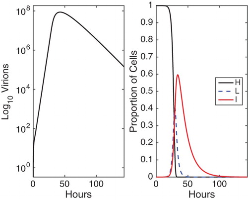
The number of virions reaches its maximum value of $8.72\times {10}^7$ virions at about 43 hours for one latent stage model, while the peak time occurs at about 46 hours for three latent stages model, with the peak value around $8.97\times {10}^7$ virions. For the fixed delay model, the peak time of number of virions occurs at around 49 hours, with the maximum number $9.06\times {10}^7$ virions. The peak times for the ODE model shifts to the right and the peak viral loads increase as the number of latent stages increases, ultimately converging to those for the DDE model as $n\to \mathrm{\infty }$ (Figure 4). We observe that with larger values of $I\left(0\right)$, peak times are observed earlier. However, the peak viral loads are not changed significantly.

Figure 4. Peak times and peak viral loads associated with different numbers of latent stages in the eclipse phase for the ODE model. The peak times and the peak viral loads increase as the number of latent stages increase. The limits of the peak times and the peak viral loads approach those of the DDE model, when $n\to \mathrm{\infty }$. Circles are for the initial conditions given in (17(17) $H\left(0\right)=6.7\times {10}^6\mathrm{cells},I\left(0\right)=6.7\mathrm{cells},$(17) ) and those marked with asterisk have initial data $V\left(0\right)=0=L\left(0\right)$ and $I\left(0\right)=20$.

5.2. CTMC simulations

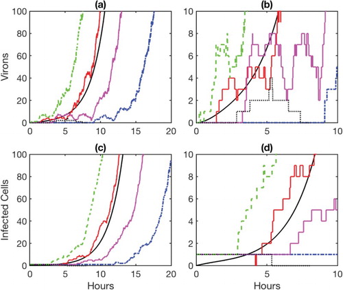
Next we consider numerical simulations of the CTMC models for one latent stage model and for three latent stage model. We use the Gillespie algorithm to compute the sample paths and define the probability of a minor infection [20]. In the simulations, a minor infection is computed as the proportion of sample paths that hit zero before reaching a predefined viral load of V =500. For one latent stage model, in a test case for $L\left(0\right)=1$ and $V\left(0\right)=0=I\left(0\right)$, the estimated probability from BP of a minor infection is 0.03. For example, in Figure 5, five sample paths for virions and infected cells are graphed over time. For initial conditions $H\left(0\right)\approx 6.7\times {10}^6$ and $L\left(0\right)=1$, the one sample path for V and I that hits zero represents a minor infection (dotted sample path in Figure 5). In this one sample path, the cell during the eclipse stage becomes infected, produces virions, and dies; the number of virions peak at about 5 hours then are cleared (dotted sample path in Figure 5(b)). However, the other four sample paths represent a major infection. On the other hand, beginning with a single virion, $V\left(0\right)=1$ and $L\left(0\right)=0=I\left(0\right)$, the BP approximate probability of a minor infection is 0.22 which agrees with the probability obtained from ${10}^4$ sample paths. As the number of host cells is sufficiently large, the BP approximation and the CTMC show good agreement [3]. Other test cases are provided in Appendix A.3.

Figure 5. Five sample paths of the CTMC model and the ODE solution (solid black curve) are graphed for virions and infected cells over time, given $L\left(0\right)=1$ and $H\left(0\right)\approx 6.7\times {10}^6$. One of the five sample paths represents a minor infection (dotted curve); vrions peak at 5 hours, then are subsequently cleared. Also, the infected cell dies shortly after 5 hours (sample path hits zero). The remaining four sample paths represent a major infection. In (a) the virion dynamics are graphed over 20 hours, and in (b) a close-up of the virion dynamics are shown over 10 hours. In (c) the infected cell dynamics are graphed for 20 hours, and in (d) a close-up of the dynamics are graphed over 10 hours. The estimate from BP yields the probability of a minor infection as 0.03.

5.3. Branching process approximation

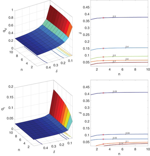
We now consider the probabilities of a minor infection computed from the BP approximation, $q_V$ and $q_I$, as functions of the transition rate β and the viral production rate b (see Figure 6). The probabilities of minor infection, $q_V$ assumes $V\left(0\right)=1$ and $I\left(0\right)=0$, whereas $q_I$ assumes $V\left(0\right)=0$ and $I\left(0\right)=1$ and $\mu =0$. All other parameters are given in Table 2. It can be seen that the probability of a minor infection decreases as the viral reproduction rate b or the transmission rate β increases. There is a much greater probability of a minor infection (clearance) with a small number of virions than with a small number of infected cells. Since $\mu =0$, the probability of a minor infection is the same for the latent stages, $q_k=q_{n+1}=q_I$ for $k=1,\dots ,n$. Contour values marked with $\ast$ in Figure 6 are in good agreement with the CTMC model (Appendix A.3).

Figure 6. Probabilities of a minor infection $q_V$, $q_I$ and contours are graphed as functions of β and b with $\mu =0$ and other parameter values given in Table 2.

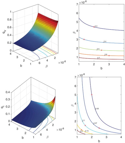
In another example, we set $\mu =0.5\times {\mu }_I=0.038$ and keep other parameters as in Table 2. The probabilities of minor infection, $q_V=q_{n+2}$ and $q_I=q_{n+1}$, are graphed as a function of the number of latent stages n and the transition rate δ in Figure 7. Contour values marked with $\ast$ in Figure 7 are in good agreement with the CTMC model (Appendix A.3). For $\mu ={\mu }_I=0.076$, the graphs are similar in shape, although the probabilities of a minor infection are greater. It can be observed that with a longer period of the eclipse phase (large $1/\delta$) as the number of latent stages increases, the probability of a minor infection increases. Also, the probability of a minor infection for $q_V$ is much greater (for a small number of virions) than for $q_I$ (for a small number of infected cells).

Figure 7. Probabilities of a minor infection $q_V$, $q_I$ and contours as functions of the number of latent stages n and transition rate δ, where the death rate $\mu =0.5\times {\mu }_I=0.038$ and other parameter values are given in Table 2.

The expressions for $q_V$ and $q_I$ in Equation (9(9) $\begin{array}{rl}{q}_k& ={\left(\frac{n\delta }{n\delta +\mu }\right)}^{n-k+1}\frac{1}{{\mathcal{R}}_0^{\left(n\right)}}+\frac{\mu }{n\delta +\mu }\sum _{l=0}^{n-k}{\left(\frac{n\delta }{n\delta +\mu }\right)}^l,\mathrm{for}k=1,2,\dots ,n,\\ q_{n+1}& =\frac{1}{{\mathcal{R}}_0^{\left(n\right)}},\\ q_{n+2}& =q_1\frac{\beta \overline{H}}{\beta \overline{H}+c}+\frac{c}{\beta \overline{H}+c}.\end{array}$(9) ) can be expressed in terms of the basic reproduction number ${\mathcal{R}}_0^{\left(0\right)}$, given in Equation (4(4) ${\mathcal{R}}_0^{\left(0\right)}=\frac{b\beta \overline{H}}{{\mu }_I(\beta \overline{H}+c)}.$(4) ). When $\mu >0$, the probabilities of a minor infection, $q_I=q_{n+1}$ and $q_V=q_{n+2}$ are (18) $\begin{array}{rl}{q}_I& =\frac{1}{{\mathcal{R}}_0^{\left(0\right)}}{\left(\frac{n\delta }{n\delta +\mu }\right)}^{-n}=\frac{1}{{\mathcal{R}}_0^{\left(0\right)}}{F}_1(\mu ,n,\delta ),\\ q_V& =\left[\frac{1}{{\mathcal{R}}_0^{\left(0\right)}}+\frac{\mu }{n\delta +\mu }\sum _{l=0}^{n-1}{\left(\frac{n\delta }{n\delta +\mu }\right)}^l\right]\frac{\beta \overline{H}}{\beta \overline{H}+c}+\frac{c}{\beta \overline{H}+c}\\ & =\left[\frac{1}{{\mathcal{R}}_0^{\left(0\right)}}+F_2(\mu ,n,\delta )\right]\frac{\beta \overline{H}}{\beta \overline{H}+c}+\frac{c}{\beta \overline{H}+c},\end{array}$(18) where (19) $F_1(\mu ,n,\delta )={\left(\frac{n\delta }{n\delta +\mu }\right)}^{-n},F_2(\mu ,n,\delta )=\frac{\mu }{n\delta +\mu }\sum _{l=0}^{n-1}{\left(\frac{n\delta }{n\delta +\mu }\right)}^l.$(19) For a latent stage $q_k$, we know that $q_V>q_k>q_I$, $k=1,\dots ,n$. As can be seen from the expressions for $F_i(\mu ,n,\delta )$, i=1,2, the probabilities of a minor infection $q_I$ and $q_V$ are increasing functions of μ and n and decreasing functions of δ (or increasing functions of $1/\delta$). Therefore, with cell death during the eclipse phase, the probability of a minor infection (no major infection) increases as the number of latent stages increases (the length of the eclipse phase increases). Evident in both Figures 6 and 7 is a marked increase in no major infection (large $q_V$ and $q_I$) with a longer eclipse phase. One implication of these results is that if drugs could target the eclipse phase and increase the value of μ the chances are greater that the infection could be cleared.

5.4. SDE and SDDE simulations

Numerical experiments of the SDE and SDDE models are performed using the Euler–Maruyama method (verified with various step sizes for accuracy) [28]. The numerical examples provide information about the variability in the number of virions at specific time points (explicit distributions are provided in the Appendix A.4). We concentrate on the time to peak viral load and compare the results to the deterministic models. Although the average length of the eclipse phase is fixed at $1/\delta =\tau =3.2$ hours, there is much variability in the time to peak, dependent on number of stages and the initial viral dose. For the initial condition as in (17(17) $H\left(0\right)=6.7\times {10}^6\mathrm{cells},I\left(0\right)=6.7\mathrm{cells},$(17) ) and for parameter values in Table 2 for ${10}^4$ sample paths, the one latent stage SDE and SDDE models have mean peak times around 43 and 48 hours, respectively. The calculated standard deviations are 0.502 and 0.592 hours, respectively. With the relatively short length of the latent stage of 3.2 hours, the variabilities in peak times cannot be neglected (Figure 8 shows the mean values and the standard deviations of peak times in the SDE/SDDE models with 1 latent stage, 2 latent stages and up to 5 latent stages and fixed delay). If the initial conditions for $I\left(0\right)=0$ and the viral dose is increased to either $V\left(0\right)=100$ or 1000, earlier peak times are obtained and the standard deviation decreases. For the one latent stage SDE model, the mean peak times for the two different viral doses are 40.8 and 36.1 hours, whereas the standard deviations are 0.326 and 0.108 hours, respectively. For the SDDE model, the mean peak times are 46.8 and 40.8 hours, and the corresponding standard deviations are 0.414 and 0.133 hours, respectively. As the length of the eclipse phase increases so does the time to viral peak.

Figure 8. The left graph shows mean values of peak times and the corresponding standard deviations with different numbers of latent stages, n=1,2,3,4,5, and a fixed delay. The standard deviations are all approximately 0.5 hours. The right graph shows mean values and the corresponding standard deviations of peak viral load. The standard deviations are small ($\approx {10}^4$) as compared with the means ($\approx {10}^7$).

6. Summary and discussion

The impact of delay in viral reproduction during the eclipse phase in deterministic and in stochastic within-host models is investigated. In particular, the models are used to study the impact of delay on the probability of a minor infection, the time to peak viral load, and the peak viral load. Inclusion of multiple stages during the eclipse phase allows for a more general distribution for this delay. The stochastic models account for the variability in viral establishment and in the peak viral load. The models are restricted to the target-cell limited model, without an immune response.

For comparison purposes, it is assumed that the average length of the eclipse phase is $1/\delta$, which is the same for all models when the eclipse-phase cells do not die over the time period of the infection (e.g. in vitro experiment). Our models show that the mean length of the eclipse phase is insufficient to determine the mean time to peak infection or mean peak viral load. For a fixed mean length of the eclipse phase, the time to peak viral load and peak viral load increases as the number of latent stages increases (Figures 4 and 8). The particular distribution associated with the eclipse phase is important, as demonstrated by others as well (e.g. [10,13,14,23,26,33]).

We apply a BP approximation of the CTMC model to estimate the probability of a minor infection, whether an infection is cleared rapidly. The greatest variability in a within-host infection occurs at the initiation of the infection process (Figure 5). Whether the infection becomes established depends on initial numbers of infected cells, eclipse-phase cells, or virions, as given in Equation (10(10) $\left(\prod _{k=1}^n{q}_k^{l_{k_0}}\right)q_{n+1}^{i_0}{q}_{n+2}^{v_0}.$(10) ). If the basic reproduction number ${\mathcal{R}}_0^{\left(n\right)}<1$, the infection will not become established, i.e. the patient recovers with relatively minor symptoms. But if the basic reproduction number ${\mathcal{R}}_0^{\left(n\right)}>1$, there is a positive probability of a major infection, where the patient suffers with severe symptoms and a high viral load. Each term in the expressions for $q_k$ can be interpreted biologically. Given an equivalent number of infected or eclipse-phase cells (with death of eclipse-phase cells), our model predicts that probability of a minor infection during any stage of the eclipse phase is greater than during the infected stage, $q_{L_k}>q_I$ $(k=1,\dots ,n)$ (Figures 6 and 7). That is, the probability a major full-blown infection is less likely if the cells have not progressed to the actively reproducing cells. Therefore, our results emphasize the importance of early drug treatment for eradication of infection. Other important consequences of the length of the eclipse phase have been demonstrated in drug treatment for HIV-1. Rong et al. [39] showed that the length of the eclipse phase impacts the development of viral resistance. Optimal resistance favours a longer eclipse phase [39].

Several simplifying assumptions have been made in our target-cell limited model: one virion is responsible for infection of a host cell, homogeneous-mixing among virions and cells, all cells and virions respond in a similar fashion (constant parameters), and the innate immune response is negligible. Some more complex models have included innate immunity (antiviral effect of interferon) [40] and spatial heterogeneity (agent-based model) [12] in influenza infection. In vivo experiments for SIV indicate that much higher viral doses than expected may be required to establish an infection and in vitro experiments indicate that much of the cell death may occur during the eclipse phase [33].

To further advance theoretical modelling investigations, some generalizations may include relaxing the Markov assumption or inclusion of a variable time delay or stochastic age-of-infection. Some investigations along these lines have been initiated but they have not been applied to within-host infection. In [15], a delay-induced stochastic model is used to describe gene regulation. In addition, Banks et al. [11] considered nonlocal delays. An SDDE with a variable delay for genetic regulatory networks was formulated in [41]. An SDE model with age-structure was studied in [16]. Another possible application of our results is to apply the lower/upper bounds for peak time, in the model with one latent stage and the model with fixed delay, to determine the possible distribution of the eclipse phase in the design of in vitro experiments.

Theoretical models are important to understand the dynamics during the early stages of the infection process when therapeutic interventions may be more effective. The length and the stages in the eclipse phase may have significant impact on the effectiveness of drug treatment and the development of drug resistance [11,25,32,37,39].

Acknowledgements

Part of this research is from the unpublished PhD dissertation of KES Huff [24]. We thank the reviewers and the editor for their helpful comments on the original manuscript.

Disclosure statement

No potential conflict of interest was reported by the authors.

Additional information

Funding

This research was supported by the National Science Foundation [grant no. DMS-1517719].

Appendix

A.1. Stability of infection-free equilibrium for DDE

We linearize the DDE system at the infection-free equilibrium $(\overline{H},0,0,V_0)$ to determine the local stability of the model at the infection-free equilibrium. Local stability is determined by the characteristic equation: (A1) $(\lambda +{\mu }_I)(\lambda +(\beta \overline{H}+c\left)\right)-b\beta \overline{H}{\mathrm{e}}^{-\mu \tau }{\mathrm{e}}^{-\tau \lambda }=0.$(A1) We want to verify that the roots of Equation (A1(A1) $(\lambda +{\mu }_I)(\lambda +(\beta \overline{H}+c\left)\right)-b\beta \overline{H}{\mathrm{e}}^{-\mu \tau }{\mathrm{e}}^{-\tau \lambda }=0.$(A1) ) are all negative or have negative real part when the basic reproduction number ${\mathcal{R}}_0<1$.

Define $F(\lambda ,\tau )=(\lambda +{\mu }_I)(\lambda +(\beta \overline{H}+c\left)\right)-b\beta \overline{H}{\mathrm{e}}^{-\mu \tau }{\mathrm{e}}^{-\tau \lambda }.$ The function F is a real function of two variables λ and τ. It is obvious that $F(\lambda ,\tau )$ is an analytic function, differentiable in both λ and τ. We investigate this equation under the assumption that ${\mathcal{R}}_0<1$.

First, $F(0,\tau )={\mu }_I(\beta \overline{H}+c)[1-{\mathcal{R}}_0]>0,$ and $F_{\lambda }(\lambda ,\tau )=2\lambda +({\mu }_I+\beta \overline{H}+c)+b\beta \overline{H}\tau {\mathrm{e}}^{-\mu \tau }{\mathrm{e}}^{-\tau \lambda }>0$ for any τ. Thus, Equation (A1(A1) $(\lambda +{\mu }_I)(\lambda +(\beta \overline{H}+c\left)\right)-b\beta \overline{H}{\mathrm{e}}^{-\mu \tau }{\mathrm{e}}^{-\tau \lambda }=0.$(A1) ) has no zero root and no positive roots for any positive value of τ.

Second, we assume that Equation (A1(A1) $(\lambda +{\mu }_I)(\lambda +(\beta \overline{H}+c\left)\right)-b\beta \overline{H}{\mathrm{e}}^{-\mu \tau }{\mathrm{e}}^{-\tau \lambda }=0.$(A1) ) has a pair of purely imaginary roots $\pm \omega i$ with $\omega >0$ for some $\tau >0$. Then ω must be a positive root of the following equation: ${\omega }^4+({\mu }_I^2+(\beta \overline{H}+c{)}^2){\omega }^2+{\mu }_I^2(\beta \overline{H}+c{)}^2-(b\beta \overline{H}{\mathrm{e}}^{-\mu \tau }{)}^2=0.$ But this equation does not have positive roots when ${\mathcal{R}}_0<1$. So Equation (A1(A1) $(\lambda +{\mu }_I)(\lambda +(\beta \overline{H}+c\left)\right)-b\beta \overline{H}{\mathrm{e}}^{-\mu \tau }{\mathrm{e}}^{-\tau \lambda }=0.$(A1) ) does not have any purely imaginary roots.

Thirdly, $F(\lambda ,0)=0$ has two roots with negative real part, ${\lambda }_{1,2}$, when ${\mathcal{R}}_0<1$ which follows from the Routh-Hurwitz criteria [2]: ${\lambda }_{1,2}=\frac{-[{\mu }_I+\beta \overline{H}+c]\pm \sqrt{({\mu }_I+\beta \overline{H}+c{)}^2-4[{\mu }_I(\beta \overline{H}+c)-b\beta \overline{H}]}}{2}.$ In addition, $F_{\lambda }({\lambda }_{1,2},0)\ne 0$. By the implicit function theorem and the continuity of the function $F(\lambda ,\tau )$, we know that all roots of Equation (A1(A1) $(\lambda +{\mu }_I)(\lambda +(\beta \overline{H}+c\left)\right)-b\beta \overline{H}{\mathrm{e}}^{-\mu \tau }{\mathrm{e}}^{-\tau \lambda }=0.$(A1) ) have negative real part for any $\tau >0$.

The conclusion is that the infection-free equilibrium of model (7(7) $\begin{array}{rl}\frac{\mathrm{d}L\left(t\right)}{\mathrm{d}t}& =\beta V\left(t\right)H\left(t\right)-\beta V(t-\tau )H(t-\tau ){\mathrm{e}}^{-\mu \tau }-\mu L\left(t\right)\\ \frac{\mathrm{d}I\left(t\right)}{\mathrm{d}t}& =\beta V(t-\tau )H(t-\tau ){\mathrm{e}}^{-\mu \tau }-{\mu }_{I}I\left(t\right),\end{array}$(7) ) is locally asymptotically stable when ${\mathcal{R}}_0<1$.

A.2. Limiting fixed point for BP approximation

The expressions given in (9(9) $\begin{array}{rl}{q}_k& ={\left(\frac{n\delta }{n\delta +\mu }\right)}^{n-k+1}\frac{1}{{\mathcal{R}}_0^{\left(n\right)}}+\frac{\mu }{n\delta +\mu }\sum _{l=0}^{n-k}{\left(\frac{n\delta }{n\delta +\mu }\right)}^l,\mathrm{for}k=1,2,\dots ,n,\\ q_{n+1}& =\frac{1}{{\mathcal{R}}_0^{\left(n\right)}},\\ q_{n+2}& =q_1\frac{\beta \overline{H}}{\beta \overline{H}+c}+\frac{c}{\beta \overline{H}+c}.\end{array}$(9) ) are used to compute the average probabilities. $\begin{array}{rl}\sum _{k=1}^n{q}_k& =\sum _{k=1}^n\left[{\left(\frac{n\delta }{n\delta +\mu }\right)}^{n-k+1}\frac{1}{{\mathcal{R}}_0^{\left(n\right)}}+\frac{\mu }{n\delta +\mu }\sum _{l=0}^{n-k}{\left(\frac{n\delta }{n\delta +\mu }\right)}^l\right]\\ & =\sum _{k=1}^n\left[{\left(\frac{n\delta }{n\delta +\mu }\right)}^{n-k+1}{\left(\frac{n\delta +\mu }{n\delta }\right)}^n\frac{{\mu }_I(\beta \overline{H}+c)}{\beta \overline{H}b}+\frac{\mu }{n\delta +\mu }\frac{1-{\left(\frac{n\delta }{n\delta +\mu }\right)}^{n-k+1}}{1-\frac{n\delta }{n\delta +\mu }}\right]\\ & =\sum _{k=1}^n\left[{\left(\frac{n\delta }{n\delta +\mu }\right)}^{-k+1}\frac{{\mu }_I(\beta \overline{H}+c)}{\beta \overline{H}b}+1-{\left(\frac{n\delta }{n\delta +\mu }\right)}^{n-k+1}\right]\\ & =\sum _{k=1}^n\left[{\left(\frac{n\delta }{n\delta +\mu }\right)}^{-k+1}\left[\frac{{\mu }_I(\beta \overline{H}+c)}{\beta \overline{H}b}-{\left(\frac{n\delta }{n\delta +\mu }\right)}^n\right]+1\right]\\ & =\sum _{k=1}^n{\left(\frac{n\delta }{n\delta +\mu }\right)}^{-k+1}\left[\frac{{\mu }_I(\beta \overline{H}+c)}{\beta \overline{H}b}-{\left(\frac{n\delta }{n\delta +\mu }\right)}^n\right]+\sum _{k=1}^{n}1\\ & =\sum _{k=0}^{n-1}{\left(\frac{n\delta }{n\delta +\mu }\right)}^{-k+2}\left[\frac{{\mu }_I(\beta \overline{H}+c)}{\beta \overline{H}b}-{\left(\frac{n\delta }{n\delta +\mu }\right)}^n\right]+n\\ & =\left[\frac{{\mu }_I(\beta \overline{H}+c)}{\beta \overline{H}b}-{\left(\frac{n\delta }{n\delta +\mu }\right)}^n\right]{\left(\frac{n\delta }{n\delta +\mu }\right)}^2\sum _{k=0}^{n-1}{\left(\frac{n\delta }{n\delta +\mu }\right)}^{-k}+n\\ & =\left[\frac{{\mu }_I(\beta \overline{H}+c)}{\beta \overline{H}b}-{\left(\frac{n\delta }{n\delta +\mu }\right)}^n\right]{\left(\frac{n\delta }{n\delta +\mu }\right)}^2\sum _{k=0}^{n-1}{\left(\frac{n\delta +\mu }{n\delta }\right)}^k+n\\ & =\left[\frac{{\mu }_I(\beta \overline{H}+c)}{\beta \overline{H}b}-{\left(\frac{n\delta }{n\delta +\mu }\right)}^n\right]{\left(\frac{n\delta }{n\delta +\mu }\right)}^2\frac{1-{\left(\frac{n\delta +\mu }{n\delta }\right)}^n}{1-\left(\frac{n\delta +\mu }{n\delta }\right)}+n\\ & =\left[\frac{{\mu }_I(\beta \overline{H}+c)}{\beta \overline{H}b}-{\left(\frac{n\delta }{n\delta +\mu }\right)}^n\right]{\left(\frac{n\delta }{n\delta +\mu }\right)}^2\left({\left(\frac{n\delta +\mu }{n\delta }\right)}^n-1\right)\frac{n\delta }{\mu }+n.\end{array}$ Let $q_L=\underset{n\to \mathrm{\infty }}{lim}\left(\sum _{k=1}^n{q}_k/n\right)$, $q_I=\underset{n\to \mathrm{\infty }}{lim}{q}_{n+1}$ and $q_V=\underset{n\to \mathrm{\infty }}{lim}{q}_{n+2}$. Then $\begin{array}{rl}{q}_L& =\underset{n\to \mathrm{\infty }}{lim}\left\{\left[\frac{{\mu }_I(\beta \overline{H}+c)}{\beta \overline{H}b}-{\left(\frac{n\delta }{n\delta +\mu }\right)}^n\right]{\left(\frac{n\delta }{n\delta +\mu }\right)}^2\left({\left(\frac{n\delta +\mu }{n\delta }\right)}^n-1\right)\frac{\delta }{\mu }+1\right\}\\ & =\left(\frac{{\mu }_I(\beta \overline{H}+c)}{\beta \overline{H}b}-{\mathrm{e}}^{-\mu /\delta }\right)\left({\mathrm{e}}^{\mu /\delta }-1\right)\frac{\delta }{\mu }+1.\end{array}$ From the definition ${\mathcal{R}}_0^{\left(d\right)}=b\beta \overline{H}{\mathrm{e}}^{-\mu /\delta }/{\mu }_I(\beta \overline{H}+c)$ in (8(8) ${\mathcal{R}}_0^{\left(d\right)}=\frac{b\beta \overline{H}{\mathrm{e}}^{-\mu /\delta }}{{\mu }_I(\beta \overline{H}+c)}={\mathcal{R}}_0^{\left(0\right)}{\mathrm{e}}^{-\mu /\delta }.$(8) ), (A2) $q_L=1-\frac{\delta }{\mu }\left(1-{\mathrm{e}}^{-\mu /\delta }\right)\left(1-\frac{1}{{\mathcal{R}}_0^{\left(d\right)}}\right)$(A2) and (A3) $q_I=\underset{n\to \mathrm{\infty }}{lim}\frac{1}{{\mathcal{R}}_0^{\left(n\right)}}=\frac{1}{{\mathcal{R}}_0^{\left(d\right)}}.$(A3) Applying the identity for $q_1$ from (9(9) $\begin{array}{rl}{q}_k& ={\left(\frac{n\delta }{n\delta +\mu }\right)}^{n-k+1}\frac{1}{{\mathcal{R}}_0^{\left(n\right)}}+\frac{\mu }{n\delta +\mu }\sum _{l=0}^{n-k}{\left(\frac{n\delta }{n\delta +\mu }\right)}^l,\mathrm{for}k=1,2,\dots ,n,\\ q_{n+1}& =\frac{1}{{\mathcal{R}}_0^{\left(n\right)}},\\ q_{n+2}& =q_1\frac{\beta \overline{H}}{\beta \overline{H}+c}+\frac{c}{\beta \overline{H}+c}.\end{array}$(9) ), $\begin{array}{rl}{q}_V& =\underset{n\to \mathrm{\infty }}{lim}{q}_{n+2}=\underset{n\to \mathrm{\infty }}{lim}{q}_1\frac{\beta \overline{H}}{\beta \overline{H}+c}+\frac{c}{\beta \overline{H}+c}\\ & =\underset{n\to \mathrm{\infty }}{lim}\left({\left(\frac{n\delta }{n\delta +\mu }\right)}^n\frac{1}{{\mathcal{R}}_0^{\left(n\right)}}+\frac{\mu }{n\delta +\mu }\sum _{l=0}^{n-1}{\left(\frac{n\delta }{n\delta +\mu }\right)}^l\right)\frac{\beta \overline{H}}{\beta \overline{H}+c}+\frac{c}{\beta \overline{H}+c}\\ & =\underset{n\to \mathrm{\infty }}{lim}\left(\frac{{\mu }_I(\beta \overline{H}+c)}{\beta \overline{H}b}+\frac{\mu }{n\delta +\mu }\frac{1-{\left(\frac{n\delta }{n\delta +\mu }\right)}^n}{1-\frac{n\delta }{n\delta +\mu }}\right)\frac{\beta \overline{H}}{\beta \overline{H}+c}+\frac{c}{\beta \overline{H}+c}\\ & =\underset{n\to \mathrm{\infty }}{lim}\left(\frac{{\mu }_I(\beta \overline{H}+c)}{\beta \overline{H}b}+1-{\left(\frac{n\delta }{n\delta +\mu }\right)}^n\right)\frac{\beta \overline{H}}{\beta \overline{H}+c}+\frac{c}{\beta \overline{H}+c}\\ & =\left(\frac{{\mu }_I(\beta \overline{H}+c)}{\beta \overline{H}b}+1-{\mathrm{e}}^{-\mu /\delta }\right)\frac{\beta \overline{H}}{\beta \overline{H}+c}+\frac{c}{\beta \overline{H}+c}\\ & =\frac{{\mu }_I}{b}+\frac{\beta \overline{H}}{\beta \overline{H}+c}-\frac{\beta \overline{H}{\mathrm{e}}^{-\mu /\delta }}{\beta \overline{H}+c}+\frac{c}{\beta \overline{H}+c}.\end{array}$ Finally, (A4) $q_V=\frac{{\mu }_I}{b}+\frac{\beta \overline{H}(1-{\mathrm{e}}^{-\mu /\delta })+c}{\beta \overline{H}+c}.$(A4)

A.3. Branching process approximation of the CTMC model

To verify the BP analytical estimates on probability of a minor infection near the infection-free equilibrium, the proportion of ${10}^4$ sample paths of the CTMC model that hit zero (before reaching $V=500$) is compared to the BP estimate in Tables 3 and 4. Parameter values come from Table 2 and Figures 6 or 7.

Table A1. Probabilities of a minor infection from the BP analytical estimate, either $q_V$ or $q_I$ (Figure 6), are compared with the proportion of ${10}^4$ sample paths that hit zero in the CTMC model.

Initial values		Parameter values		BP or CTMC
$I\left(0\right)$	$V\left(0\right)$	β	b	$q_V$ or $q_I$	Proportion	Error${}^{\mathrm{a}}$
0	1	$4.4\times {10}^{-8}$	2.0	0.300	0.309	0.005
0	1	$3.0\times {10}^{-8}$	1.3	0.400	0.393	0.005
0	1	$1.8\times {10}^{-8}$	2.5	0.500	0.503	0.005
0	1	$1.2\times {10}^{-8}$	3.0	0.600	0.597	0.005
1	0	$3.5\times {10}^{-8}$	1.32	0.050	0.055	0.002
1	0	$5.0\times {10}^{-8}$	1.31	0.070	0.069	0.003
1	0	$5.0\times {10}^{-8}$	1.96	0.100	0.103	0.003
1	0	$3.5\times {10}^{-8}$	1.99	0.150	0.148	0.004

${}^{\mathrm{a}}$ Standard error for the proportion.

Table A2. Probabilities of a minor infection from the BP analytical estimate, either $q_V$ or $q_I$ (n=3 in Figure 7), are compared with the proportion of ${10}^4$ sample paths that hit zero in the CTMC model.

Initial values		Parameter values	BP or CTMC
$I\left(0\right)$	$V\left(0\right)$	δ	$q_V$ or $q_I$	Proportion	Error${}^{\mathrm{a}}$
0	1	0.37	0.300	0.303	0.005
0	1	0.15	0.400	0.393	0.005
0	1	0.08	0.400	0.496	0.005
0	1	0.06	0.600	0.591	0.005
1	0	0.41	0.030	0.031	0.002
1	0	0.10	0.040	0.039	0.002
1	0	0.07	0.045	0.045	0.002
1	0	0.03	0.070	0.073	0.003

${}^{\mathrm{a}}$ Standard error for the proportion.

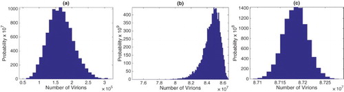
Figure A.1. Approximate pdfs for number of virions at (a) time 20 hours, (b) 40 hours, and (c) peak of the viral load for the SDE model with one stage in the eclipse phase. The approximate pdfs are computed from ${10}^4$ sample paths. Initial conditions are given in (17(17) $H\left(0\right)=6.7\times {10}^6\mathrm{cells},I\left(0\right)=6.7\mathrm{cells},$(17) ).

A.4. Statistical summary for SDE and SDDE models

For the SDE model with one stage in the eclipse stage, approximations for the pdfs for the number of virions at 20 and 40 hours are graphed in Figure A1. Statistical summaries for the mean, standard deviation, skewness, and kurtosis are given in Table 5. Similar histograms at 20 and 40 hours for the SDDE model are graphed in Figure A2 and the relevant statistical data are summarized in Table 6. All results are computed from ${10}^4$ sample paths. In the SDE and SDDE models, the pdfs at hours prior to the peak time exhibit positive skewness, whereas after the peak time, they exhibit negative skewness. If the initial number of infected cells or number of virions is not a fixed value but has given probability distribution, as expected, the variability is also increased (see Appendix A.4 for an example).

Table A3. SDE Statistical summary for the viral load (virions) of the model with one stage in the eclipse phase at times 10, 20, 30, 40, 50, and 60 hours with initial conditions given in (17(17) $H\left(0\right)=6.7\times {10}^6\mathrm{cells},I\left(0\right)=6.7\mathrm{cells},$(17) ), computed from ${10}^4$ sample paths.

	10 hours	20 hours	30 hours	40 hours	50 hours	60 hours
ODE	$1.28\times {10}^3$	$1.61\times {10}^5$	$1.91\times {10}^7$	$8.47\times {10}^7$	$7.55\times {10}^7$	$4.83\times {10}^7$
SDE Mean	$1.32\times {10}^3$	$1.65\times {10}^5$	$1.93\times {10}^7$	$8.46\times {10}^7$	$7.55\times {10}^7$	$4.84\times {10}^7$
SDE STD	$3.12\times {10}^2$	$3.91\times {10}^4$	$3.68\times {10}^6$	$1.06\times {10}^6$	$1.28\times {10}^6$	$1.28\times {10}^6$
SDE Skewness	0.372	0.373	0.010	−1.062	0.263	0.397
SDE Kurtosis	3.24	3.24	2.86	4.96	3.11	3.30

Figure A.2. Approximate pdfs for virions at (a) 20 hours, (b) 40 hours, and (c) peak times for the SDDE model. The approximate pdfs are computed from ${10}^4$ sample paths. Initial values are given in (17(17) $H\left(0\right)=6.7\times {10}^6\mathrm{cells},I\left(0\right)=6.7\mathrm{cells},$(17) ).

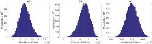
Table A4. SDDE statistical summary for the viral load (virions) at times 10, 20, 30, 40, 50, and 60 hours with initial conditions given in (17(17) $H\left(0\right)=6.7\times {10}^6\mathrm{cells},I\left(0\right)=6.7\mathrm{cells},$(17) ), computed from ${10}^4$ sample paths.

	10 hours	20 hours	30 hours	40 hours	50 hours	60 hours
DDE	$4.02\times {10}^2$	$1.96\times {10}^4$	$9.70\times {10}^5$	$4.74\times {10}^7$	$9.00\times {10}^7$	$6.61\times {10}^7$
SDDE Mean	$4.05\times {10}^2$	$1.98\times {10}^4$	$9.83\times {10}^5$	$4.68\times {10}^7$	$8.99\times {10}^7$	$6.62\times {10}^7$
SDDE STD	90.9	$4.36\times {10}^3$	$2.30\times {10}^5$	$6.54\times {10}^6$	$5.10\times {10}^5$	$1.76\times {10}^6$
SDDE Skewness	0.291	0.260	0.339	−0.431	−0.686	0.390
SDDE Kurtosis	3.11	3.06	3.20	3.15	3.33	3.29

Suppose the initial host cell population is $H\left(0\right)=6.7\times {10}^6\mathrm{cells}$ and viral load (virions) is given by a discrete probability distribution (A5) $I\left(0\right)=\left\{\begin{array}{ll}5,& p=0.18\\ 6,& p=0.2\\ 7,& p=0.4\\ 8,& p=0.22\end{array}\right.$(A5) with other initial cell populations equal to zero. The mean of $I\left(0\right)$ is 6.7 cells. The standard deviations for the distributions at later times, $t=10,\dots ,60$, are greater than the initial data for $I\left(0\right)=6.7$ and the distributions are in Tables 7 and 8.

Table A5. SDE statistical summary for viral load (virions) for the model with one latent stage at 10, 20, 30, 40, 50, and 60 hours with initial conditions $H\left(0\right)=6.7\times {10}^6$ and $I\left(0\right)$ given by (A5(A5) $I\left(0\right)=\left\{\begin{array}{ll}5,& p=0.18\\ 6,& p=0.2\\ 7,& p=0.4\\ 8,& p=0.22\end{array}\right.$(A5) ), computed from ${10}^4$ sample paths.

	10 hours	20 hours	30 hours	40 hours	50 hours	60 hours
ODE	$1.28\times {10}^3$	$1.61\times {10}^5$	$1.91\times {10}^7$	$8.47\times {10}^7$	$7.55\times {10}^7$	$4.83\times {10}^7$
SDE Mean	$1.31\times {10}^3$	$1.64\times {10}^5$	$1.91\times {10}^7$	$8.44\times {10}^7$	$7.56\times {10}^7$	$4.84\times {10}^7$
SDE STD	$3.64\times {10}^2$	$4.56\times {10}^4$	$4.33\times {10}^6$	$1.36\times {10}^6$	$1.53\times {10}^6$	$1.55\times {10}^6$
SDE Skewness	0.344	0.340	−0.061	−1.470	0.417	0.596
SDE Kurtosis	3.10	3.10	2.80	6.94	3.30	3.70

Table A6. SDDE statistical summary for viral load (virions) at 10, 20, 30, 40, 50, and 60 hours with initial conditions $H\left(0\right)=6.7\times {10}^6$ and $I\left(0\right)$ given by (A5(A5) $I\left(0\right)=\left\{\begin{array}{ll}5,& p=0.18\\ 6,& p=0.2\\ 7,& p=0.4\\ 8,& p=0.22\end{array}\right.$(A5) ), computed from ${10}^4$ sample paths.

	10 hours	20 hours	30 hours	40 hours	50 hours	60 hours
DDE	$4.02\times {10}^2$	$1.96\times {10}^4$	$9.70\times {10}^5$	$4.74\times {10}^7$	$9.00\times {10}^7$	$6.61\times {10}^7$
SDDE Mean	$4.02\times {10}^2$	$1.97\times {10}^4$	$9.76\times {10}^5$	$4.63\times {10}^7$	$8.99\times {10}^7$	$6.64\times {10}^7$
SDDE STD	$1.08\times {10}^2$	$5.34\times {10}^3$	$2.74\times {10}^5$	$7.94\times {10}^6$	$5.92\times {10}^5$	$2.16\times {10}^6$
SDDE Skewness	0.276	0.273	0.306	−0.487	−0.749	0.543
SDDE Kurtosis	2.95	2.99	2.98	3.09	3.12	3.59

References

- E. Allen, Modeling With Itô Stochastic Differential Equations, Vol. 22, Springer Science & Business Media, Dordrecht, 2007.
- L.J.S. Allen, An Introduction to Stochastic Processes with Applications to Biology, 2nd ed., CRC Press, Boca Raton, FL, 2010.
- L.J.S. Allen, Stochastic Population and Epidemic Models: Persistence and Extinction, Vol. 1.3, Mathematical Biosciences Institute Lecture Series, Springer, Cham, Switzerland, 2015.
- L.J.S. Allen, A primer on stochastic epidemic models: Formulation, numerical simulation, and analysis, Infect. Dis. Model. 2 (2017), pp. 128–142.
- L.J.S. Allen and G.E. Lahodny Jr, Extinction thresholds in deterministic and stochastic epidemic models, J. Biol. Dyn. 6(2) (2012), pp. 590–611. doi: 10.1080/17513758.2012.665502
- L.J.S. Allen and P. van den Driessche, Relations between deterministic and stochastic thresholds for disease extinction in continuous-and discrete-time infectious disease models, Math. Biosci. 243(1) (2013), pp. 99–108. doi: 10.1016/j.mbs.2013.02.006
- E.J. Allen, L.J.S. Allen, A. Arciniega, and P.E. Greenwood, Construction of equivalent stochastic differential equation models, Stoch. Anal. Appl. 26(2) (2008), pp. 274–297. doi: 10.1080/07362990701857129
- D.A. Anderson and R.K. Watson, On the spread of a disease with gamma distributed latent and infectious periods, Biometrika 67 (1980), pp. 191–198. doi: 10.1093/biomet/67.1.191
- K.B. Athreya and P.E. Ney, Branching Processes, Dover, Mineola, NY, 2004.
- P. Baccam, C.A.A. Beauchemin, C.A. Macken, F.G. Hayden, and A.S. Perelson, Kinetics of influenza A virus infection in humans, J. Virol. 80(15) (2006), pp. 7590–7599. doi: 10.1128/JVI.01623-05
- H.T. Banks, J. Catenacci, and S. Hu, Stochastic vs. deterministic models for systems with delays, IFAC Proc. Vol. 46(26) (2013), pp. 61–66. doi: 10.3182/20130925-3-FR-4043.00022
- A.L. Bauer, C.A.A. Beauchemin, and A.S. Perelson, Agent-based modeling of host–pathogen systems: The successes and challenges, Inform. Sci. 179(10) (2009), pp. 1379–1389. doi: 10.1016/j.ins.2008.11.012
- C.A.A. Beauchemin and A. Handel, A review of mathematical models of influenza A infections within a host or cell culture: Lessons learned and challenges ahead, BMC Public Health 11(1) (2011), p. S7. doi: 10.1186/1471-2458-11-S1-S7
- C.A.A. Beauchemin, J.J. McSharry, G.L. Drusano, J.T. Nguyen, G.T. Went, R.M. Ribeiro, and A.S. Perelson, Modeling amantadine treatment of influenza A virus in vitro, J. Theoret. Biol. 254 (2008), pp. 439–451. doi: 10.1016/j.jtbi.2008.05.031
- D. Bratsun, D. Volfson, L.S. Tsimring, and J. Hasty, Delay-induced stochastic oscillations in gene regulation, Proc. Natl. Acad. Sci. 102(41) (Sep 2005), pp. 14593–14598. doi: 10.1073/pnas.0503858102
- M. Chowdhury and E.J. Allen, A stochastic continuous-time age-structured population model, Nonlinear Anal. 47(3) (2001), pp. 1477–1488. doi: 10.1016/S0362-546X(01)00283-8
- S.M. Ciupe and J.M. Heffernan, In-host modeling, Infect. Dis. Model. 2 (2017), pp. 188–202.
- J.M. Conway, B.P. Konrad, and D. Coombs, Stochastic analysis of pre-and postexposure prophylaxis against HIV infection, SIAM J. Appl. Math. 73(2) (2013), pp. 904–928. doi: 10.1137/120876800
- N.M. Dixit, M. Markowitz, D.D. Ho, and A.S. Perelson, Estimates of intracellular delay and average drug efficacy from viral load data of HIV-infected individuals under antiretroviral therapy, Antivir. Ther. 9(2) (2004), pp. 237–246.
- D.T. Gillespie, Exact stochastic simulation of coupled chemical reactions, J. Phys. Chem. 81(25) (1977), pp. 2340–2361. doi: 10.1021/j100540a008
- Z. Grossman, M. Polis, M. B. Feinberg, Z. Grossman, I. Levi, S. Jankelevich, R. Yarchoan, J. Boon, F. de Wolf, J. M.A. Lange, J. Goudsmit, D. S. Dimitrov, and W. E. Paul, Ongoing HIV dissemination during HAART, Nature Med. 5(10) (1999), pp. 1099–1104. doi: 10.1038/13410
- T.E. Harris, The Theory of Branching Processes, Springer-Verlag, Berlin, 1963.
- B.P. Holder and C.A.A. Beauchemin, Exploring the effect of biological delays in kinetic models of influenza within a host or cell culture, BMC Public Health 11(Suppl. 1) (2011), pp. S10. doi: 10.1186/1471-2458-11-S1-S10
- K.E.S. Huff, Modeling the early stages of within-host viral infection and clinical progression of hantavirus pulmonary syndrome. PhD thesis, Texas Tech University, 2018.
- C.B. Jonsson, J. Hooper, and G. Mertz, Treatment of hantavirus pulmonary syndrome, Antiviral Res. 78(1) (2008), pp. 162–169. doi: 10.1016/j.antiviral.2007.10.012
- Y. Kakizoe, S. Nakaoka, C.A.A. Beauchemin, S. Morita, S. Morita, H. Mori, T. Igarashi, K. Aihara, T. Miura, and S. Iwami, A method to determine the duration of the eclipse phase for in vitro infection with a highly pathogenic SHIV strain, Sci. Rep. 5 (2015), p. 10371. doi:doi: 10.1038/srep10371.
- S. Karlin and H. Taylor, A First Course in Stochastic Processes, 2nd ed., Academic Press, New York, 1975.
- P.E. Kloeden, E. Platen, and H. Schurz, Numerical Solution of SDE Through Computer Experiments, Springer Science & Business Media, Berlin/Heidelberg, Germany, 2012.
- A.L. Lloyd, The dependence of viral parameter estimates on the assumed viral life cycle: Limitations of studies of viral load data, Proc. R. Soc. Lond. B 268(1469) (2001), pp. 847–854. doi: 10.1098/rspb.2000.1572
- A.L. Lloyd, Destabilization of epidemic models with the inclusion of realistic distributions of infectious periods, Proc. R. Soc. Lond. B 268(1470) (2001), pp. 985–993. doi: 10.1098/rspb.2001.1599
- A.L. Lloyd, Realistic distributions of infectious periods in epidemic models: Changing patterns of persistence and dynamics, Theoret. Popul. Biol. 60(1) (2001), pp. 59–71. doi: 10.1006/tpbi.2001.1525
- I.A Neagu, J. Olejarz, M. Freeman, D.I.S. Rosenbloom, M.A. Nowak, and A.L. Hill, Life cycle synchronization is a viral drug resistance mechanism, PLoS Comput. Biol. 14(2) (2018), p. e1005947. doi: 10.1371/journal.pcbi.1005947
- C. Noecker, K. Schaefer, K. Zaccheo, Y. Yang, J. Day, and V. Ganusov, Simple mathematical nodels do not accurately predict early SIV dynamics, Viruses 7(3) (2015), pp. 1189–1217. doi: 10.3390/v7031189
- J.E. Pearson, P. Krapivsky, and A.S. Perelson, Stochastic theory of early viral infection: Continuous versus burst production of virions, PLoS Comput. Biol. 7(2) (2011), p. e1001058. doi: 10.1371/journal.pcbi.1001058
- A.S. Perelson, D.E. Kirschner, and R. De Boer, Dynamics of HIV infection of CD4+ T cells, Math. Biosci. 114(1) (1993), pp. 81–125. doi: 10.1016/0025-5564(93)90043-A
- L.T. Pinilla, B.P. Holder, Y. Abed, G. Boivin, and C.A.A. Beauchemin, The H275Y neuraminidase mutation of the pandemic A/H1N1 influenza virus lengthens the eclipse phase and reduces viral output of infected cells, potentially compromising fitness in ferrets, J. Virol. 86(19) (2012), pp. 10651–10660. doi: 10.1128/JVI.07244-11
- R.M. Ribeiro, L. Qin, L.L. Chavez, D. Li, S.G. Self, and A.S. Perelson, Estimation of the initial viral growth rate and basic reproductive number during acute HIV-1 infection, J. Virol. 84(12) (2010), pp. 6096–6102. doi: 10.1128/JVI.00127-10
- M.G. Roberts and J.A.P. Heesterbeek, A new method for estimating the effort required to control an infectious disease, Proc. R. Soc. Lond. B 270 (2003), pp. 1359–1364. doi: 10.1098/rspb.2003.2339
- L. Rong, M.A. Gilchrist, Z. Feng, and A.S. Perelson, Modeling within-host HIV-1 dynamics and the evolution of drug resistance: Trade-offs between viral enzyme function and drug susceptibility, J. Theoret. Biol. 247(4) (2007), pp. 804–818. doi: 10.1016/j.jtbi.2007.04.014
- R.A. Saenz, M. Quinlivan, D. Elton, S. MacRae, A.S. Blunden, J.A. Mumford, J.M. Daly, P. Digard, A. Cullinane, B.T. Grenfell, J.W. McCauley, J.L.N. Wood, and J.R. Gog, Dynamics of influenza virus infection and pathology, J. Virol. 84(8) (2010), pp. 3974–3983. doi: 10.1128/JVI.02078-09
- T. Tian, K. Burrage, P.M. Burrage, and M. Carletti, Stochastic delay differential equations for genetic regulatory networks, J. Comput. Appl. Math. 205(2) (2007), pp. 696–707. doi: 10.1016/j.cam.2006.02.063
- H.C. Tuckwell and E. Le Corfec, A stochastic model for early HIV-1 population dynamics, J. Theoret. Biol. 195(4) (1998), pp. 451–463. doi: 10.1006/jtbi.1998.0806
- H.C. Tuckwell and F.Y.M. Wan, First passage time to detection in stochastic population dynamical models for HIV-1, Appl. Math. Lett. 13(5) (2000), pp. 79–83. doi: 10.1016/S0893-9659(00)00037-9
- P. van den Driessche and J. Watmough, Reproduction numbers and sub-threshold endemic equilibria for compartmental models of disease transmission, Math. Biosci. 180(1) (2002), pp. 29–48. doi: 10.1016/S0025-5564(02)00108-6
- P. Whittle, The outcome of a stochastic epidemic–a note on Bailey's paper, Biometrika 42 (1955), pp. 116–122.
- A.W.C. Yan, P. Cao, and J.M. McCaw, On the extinction probability in models of within-host infection: The role of latency and immunity, J. Math. Biol. 73 (2016), pp. 787–813. doi: 10.1007/s00285-015-0961-5
- Y. Yuan and L.J.S. Allen, Stochastic models for virus and immune system dynamics, Math. Biosci. 234(2) (2011), pp. 84–94. doi: 10.1016/j.mbs.2011.08.007