Characterization of Wolbachia enhancing domain in mosquitoes with imperfect maternal transmission

ABSTRACT

A novel method to reduce the burden of dengue is to seed wild mosquitoes with Wolbachia-infected mosquitoes in dengue-endemic areas. Concerns in current mathematical models are to locate the Wolbachia introduction threshold. Our recent findings manifest that the threshold is highly dependent on the initial population size once Wolbachia infection alters the logistic control death rate of infected females. However, counting mosquitoes is beyond the realms of possibility. A plausible method is to monitor the infection frequency. We propose the concept of Wolbachia enhancing domain in which the infection frequency keeps increasing. A detailed description of the domain is presented. Our results suggest that both the initial population size and the infection frequency should be taken into account for optimal release strategies. Both Wolbachia fixation and extinction permit the oscillation of the infection frequency.

KEYWORDS:

• Wolbachia
• cytoplasmic incompatibility
• population replacement
• enhancing domain
• shadow point

1. Introduction

The ability of Wolbachia to spread through cytoplasmic incompatibility (CI) [33,36] and grant mosquitoes resistant to dengue virus [2,21] has triggered the development of Wolbachia-based strategies for population replacement of Aedes mosquitoes, the primary vectors of dengue. Since 2009, small-scale trials have been conducted in dengue-affected communities, including Australia, Vietnam, Brazil and Colombia [10,11]. Before the implement of large-scale trials, one major concern is the introduction threshold of Wolbachia-infected individuals that must be surpassed for infection to spread and become established in the population.

Several key parameters are critical for determining the introduction threshold. (i) The intensity of CI $s_h$, which is the probability of embryo death from the crossing of infected males with uninfected females; (ii) The maternal transmission leakage $\mu \in [0,1]$, which is the percentage of uninfected progeny produced by an infected mother. (iii) The fitness cost/benefit, including changes in fecundity, hatching, pupation, eclosing and adult longevity, of infected females caused by Wolbachia infection. The classical finding of Turelli–Hoffman [29,31,32] on Wolbachia invasion in Drosophila simulans, based on discrete models parameterized using laboratory and field data, showed that the dynamics of Wolbachia spread can be determined completely by the frequency of infected among all individuals $p\left(t\right)$. They showed that there is a unique threshold of the infection frequency $p^{\ast }\in (0,1)$: If the initial infection frequency $p\left(0\right)>p^{\ast }$, then $p\left(t\right)$ increases for all t>0 and $p\left(t\right)\to 1$ as $t\to \mathrm{\infty }$ for Wolbachia fixation; if $p\left(0\right)<p^{\ast }$, then $p\left(t\right)$ decreases for all t<0 with $p\left(t\right)\to 0$ as $t\to \mathrm{\infty }$ to drive Wolbachia extinction. Such a simple correspondence between the infection frequency and Wolbachia spreading dynamics has been justified repeatedly for laboratory experiments of mosquitoes with separated generations [6,10,36].

However, for Wobachia spread in a natural setting where mosquitoes are present in overlapping generations, the situation is much more complicated. Various mathematical models have been developed to characterize the thresholds, including models of ordinary differential equations [16,22,38–40], delay differential equations [15,39], impulsive differential equations [37], stochastic equations [12], and reaction-diffusion equations [13,14,30]. In most of the above theoretical studies on characterization of the introduction thresholds, it was assumed that the maternal transmission is perfect ($\mu =0$) and CI is complete ($s_h=1$), which are supported by Wolbachia strain WB1 in Aedes aegypti [36], wAlbA and wAlbB in Aedes albopictus [35]. Although imperfect maternal transmission $(\mu >0$) has been repeatedly documented with respect to the wRi, wRu infection in D. simulans [5,17,18,32] and the wMel in Drosophila melanogaster [9], It was predominantly believed that the maternal transmission of Wolbachia in mosquitoes is perfect. However, a very recent study [26] demonstrates that high temperatures (26–37${}^{\circ }\mathrm{C}$) can induce both imperfect maternal transmission of Wolbachia in A. aegypti, the primary vector of dengue. Imperfect maternal transmission was also observed in a recent study on the spread of Wolbachia strain LB1 in Anopheles stephensi [3].

Motivated by these findings, we developed models of ordinary differential equations in [40,41] to describe Wolbachia spreading dynamics, aiming to understand the effect of imperfect maternal transmission. To the end, let $I\left(t\right)$ and $U\left(t\right)$ be respectively the population size of infected and uninfected adults at time t, both equally distributed in sex. Let $b_I$ (or $b_U$) be the natural birth rate of infected (or uninfected) individuals. As infected offsprings are born only from infected mothers, by taking the maternal transmission leakage into account, the birth of infected offsprings reads as $b_I(1-\mu )I/2$. The birth function of uninfected offsprings is $\frac{b_I}{2}\mu I+\frac{b_U}{2}U\cdot \left(1-\frac{I}{I+U}\right),$ in which the first term accounts for the leakage of infected mothers, and the second term is from uninfected mothers, with the CI intensity $s_h=1$ for matings between uninfected females and infected males. On the loss of mosquitoes, we follow the conventional approach by replacing the natural death of adults with a logistic-like density dependence term, which increases in I (or U) and the sum I+U. Let ${\delta }_I$ (or ${\delta }_U$) be the logistic control coefficient for infected (or uninfected) mosquitoes. The loss of reproduction due to density dependent death is modelled by ${\delta }_{I}I(I+U)$ (or ${\delta }_{U}U(I+U)$) for infected (or uninfected) mosquitoes. In summary, our model takes the form (1) $\frac{\mathrm{d}I}{\mathrm{d}t}=\frac{1}{2}{b}_I(1-\mu )I-{\delta }_{I}I(I+U),$(1) (2) $\frac{\mathrm{d}U}{\mathrm{d}t}=\frac{1}{2}{b}_I\mu I+\frac{b_U{U}^2}{2(I+U)}-{\delta }_{U}U(I+U).$(2) Upon the rescaling (3) $x=\frac{2{\delta }_U}{b_U}I,y=\frac{2{\delta }_U}{b_U}U,s=\frac{b_U}{2}t,\beta =\frac{b_I}{b_U},\delta =\frac{{\delta }_I}{{\delta }_U},$(3) and rewriting $\mathrm{d}\cdot /\mathrm{d}s$ as $\mathrm{d}\cdot /\mathrm{d}t$, system (1(1) $\frac{\mathrm{d}I}{\mathrm{d}t}=\frac{1}{2}{b}_I(1-\mu )I-{\delta }_{I}I(I+U),$(1) ) and (2(2) $\frac{\mathrm{d}U}{\mathrm{d}t}=\frac{1}{2}{b}_I\mu I+\frac{b_U{U}^2}{2(I+U)}-{\delta }_{U}U(I+U).$(2) ) is reduced into (4) $\frac{\mathrm{d}x}{\mathrm{d}t}=\beta (1-\mu )x-\delta x(x+y):=f(x,y),$(4) (5) $\frac{\mathrm{d}y}{\mathrm{d}t}=\beta \mu x+\frac{y^2}{x+y}-y(x+y):=g(x,y),$(5) where β (or δ) is the birth (or death) rate constant of infected females relative to uninfected females, and x, y are respectively the rescaled population size of infected and uninfected individuals.

Our recent studies [40,41] showed that system (4(4) $\frac{\mathrm{d}x}{\mathrm{d}t}=\beta (1-\mu )x-\delta x(x+y):=f(x,y),$(4) ) and (5(5) $\frac{\mathrm{d}y}{\mathrm{d}t}=\beta \mu x+\frac{y^2}{x+y}-y(x+y):=g(x,y),$(5) ) exhibits monomorphic, bistable, and polymorphic dynamics. A detailed description of the threshold curve is offered in terms of β, μ and δ, as we have done for perfect maternal transmission case in [39]. The results suggest that the largest maternal transmission leakage rate supporting possible Wolbachia spreading does not necessarily increase with the fitness of infected mosquitoes. By exploring the analytical property of the threshold curve, we find that with the presence of imperfect maternal transmission rate, Wolbachia in a completely infected population could be wiped out ultimately if the initial population size is small. All these findings point to the fact that even when $\mu =0$ which corresponds to perfect maternal transmission, there is no more single threshold infection frequency unless $\delta =1$, and the classical result of Turelli–Hoffman needs to be interpreted differently. Indeed, we showed that there is a threshold curve, depending on the initial population sizes of both infected and uninfected mosquitoes when $\delta \ne 1$. Although we offered a complete classification of the Wolbachia infection dynamics by the proof of a unique threshold curve, the separatrix of an unstable saddle point, the implication of results requires a knowledge of the initial population sizes $x\left(0\right)$ and $y\left(0\right)$. This is, practically, a formidable task in large areas with complex landscape structures, in particular, in residential areas. On the other hand, the infection frequency may be estimated by undertaking PCR assay on samples or progeny tests on subsamples from various locations [32]. To make our theoretical results be more helpful in surveillance and adjustment of release strategies, here, we proposed the concept of Enhancing domain in terms of the growth rate of the Wolbachia infection frequency $p\left(t\right)=x\left(t\right)/\left[x\right(t)+y(t\left)\right]$ which is determined by $p^{\mathrm{\prime }}\left(t\right)=\frac{yf(x,y)-xg(x,y)}{\left(x\right(t)+y(t){)}^2}.$ For a single point $(x,y)\in {\mathbb{E}}^o:=\left\{\right(x,y):x\ge 0,y\ge 0\}$, define (6) ${\mathbb{E}}^I=\left\{\right(x,y):x,y>0,yf(x,y)>xg(x,y\left)\right\},$(6) which consists of all points $(x,y)$ at which the infection frequency increases. We call ${\mathbb{E}}^I$ the Wolbachia infection enhancing domain in which infected mosquitoes is more favoured comparing to uninfected ones. The aim of this paper is to characterize $E^I$ and elucidate the relation or most importantly, the difference between the enhancing domain and the attraction domain of Wolbachia fixation equilibrium, denoted by $A^I$. Our results show that, when $\delta \ne 1$ or $\mu \ne 0$, the relative complement of $E^I$ in $A^I$ is not empty, which implies that the infection frequency could go to Wolbachia fixation even though it does not always increase. Meanwhile, the relative complement of $A^I$ in $E^I$ is not empty either, in which initially, the infection frequency increases, but eventually, Wolbachia will go to extinction. These deceptive phenomena should be taken into account when designing release strategies to guarantee the success.

2. Preliminaries

When the maternal transmission of Wolbachia is perfect and the infection does not affect the lifespan of infected females, i.e. $\mu =0$, and $\delta =1.$ From (4(4) $\frac{\mathrm{d}x}{\mathrm{d}t}=\beta (1-\mu )x-\delta x(x+y):=f(x,y),$(4) ) and (5(5) $\frac{\mathrm{d}y}{\mathrm{d}t}=\beta \mu x+\frac{y^2}{x+y}-y(x+y):=g(x,y),$(5) ), we have $\begin{array}{rl}\frac{\mathrm{d}p}{\mathrm{d}t}& =\frac{\mathrm{d}}{\mathrm{d}t}\left(\frac{x}{x+y}\right)\\ & =\frac{1}{x+y}\cdot \frac{\mathrm{d}x}{\mathrm{d}t}-\frac{x}{(x+y{)}^2}\cdot \left(\frac{\mathrm{d}x}{\mathrm{d}t}+\frac{\mathrm{d}y}{\mathrm{d}t}\right)\\ & =\beta p-x-p[\beta p-x+(1-p{)}^2-y]\\ & =\beta p-\beta p^2-p(1-p{)}^2\\ & =p(p+\beta -1)(1-p).\end{array}$ If $\beta >1$, then $\mathrm{d}p/\mathrm{d}t>0$ always holds, and hence $E^I=E^o$. If $\beta <1$, then the infection frequency presents an Allee effect: $p\left(t\right)$ goes to 1 for Wolbachia fixation when $p\left(0\right)>p^{\ast }:=1-\beta$, and to 0 for Wolbachia extinction when $p\left(0\right)<p^{\ast }$. In this case, $E^I=\left\{(x,y):\frac{x}{x+y}>p^{\ast }\right\}=\left\{(x,y):y<\frac{\beta }{1-\beta }x\right\}.$

Noticing that system (4(4) $\frac{\mathrm{d}x}{\mathrm{d}t}=\beta (1-\mu )x-\delta x(x+y):=f(x,y),$(4) )and (5(5) $\frac{\mathrm{d}y}{\mathrm{d}t}=\beta \mu x+\frac{y^2}{x+y}-y(x+y):=g(x,y),$(5) ) admits no interior equilibrium when $\beta >1$, and a unique interior equilibrium $E^{\ast }(x^{\ast },y^{\ast })=(\beta -{\beta }^2,{\beta }^2)$ when $\beta <1$, combining the characterization of $A^I$ in [39] (Theorem 2.1), we can conclude that the enhancing domain is identical to the attracting basin of Wolbachia fixation equilibrium $(\beta ,0)$ when $\beta <1$. In summary, we have $E^I=A^I\mathrm{for}\mu =0\mathrm{and}\delta =1.$ However, things are quite different for $\mu \ne 0$ or $\delta \ne 1$. Since $yf(x,y)>xg(x,y)⟺\delta xy(x+y)<\beta (1-\mu )xy-xg(x,y),$ and $g(x,y)$ is independent of δ, we have the following simple monotone properties (7) $0<{\delta }_1<{\delta }_2⟹{\mathbb{E}}^I{|}_{\delta ={\delta }_1}\supset {\mathbb{E}}^I{|}_{\delta ={\delta }_2}.$(7)

In order to identify the domain ${\mathbb{E}}^I$ in a systematic way, we introduce, for fixed constants c>0, $l_c\left(t\right):=cx\left(t\right)-y\left(t\right).$ We denote by $L_c$ the ray $y=cx,x>0$. If $\gamma \left(t\right)=\left(x\right(t),y(t\left)\right)\in L_c$ for some $t\ge 0$, then $l_c\left(t\right)=0$. If it is additionally known that $l_c^{\mathrm{\prime }}\left(t\right)>0$, then $l_c\left(s\right)>0$ for all s sufficiently close to t with s>t, implying that $y\left(s\right)/x\left(s\right)<c=y\left(t\right)/x\left(t\right)⟹p\left(s\right)>p\left(t\right).$ A similar argument shows that $p\left(s\right)<p\left(t\right)$ for all s sufficiently close to t and s<t. As a result, $p\left(t\right)$ increases near t when $l_c^{\mathrm{\prime }}\left(t\right){|}_{L_c}>0$. Similarly, $p\left(t\right)$ decreases near t when $l_c^{\mathrm{\prime }}\left(t\right){|}_{L_c}<0$.

For $(x,y)\in {\mathbb{E}}^o$, the line connecting it with the origin cuts the $x-$nullcline ${\mathrm{\Gamma }}_x:x+y=\kappa :=\frac{\beta (1-\mu )}{\delta }$ exactly once. We denote by $(x_s,y_s)$ the unique cutting point, and call it the shadow point of $(x,y)$ on ${\mathrm{\Gamma }}_x$. If $(x,y)$ is itself on the nullcline, then it coincides with its shadow. In general, $(x,y)$ and its shadow point are colinear with the origin, and $x_s=x_s(x,y)=\frac{\kappa x}{x+y},\mathrm{and}{y}_s=y_s(x,y)=\frac{\kappa y}{x+y}.$ For a solution $\gamma \left(t\right)=\left(x\right(t),y(t\left)\right)$ of (4(4) $\frac{\mathrm{d}x}{\mathrm{d}t}=\beta (1-\mu )x-\delta x(x+y):=f(x,y),$(4) ) and (5(5) $\frac{\mathrm{d}y}{\mathrm{d}t}=\beta \mu x+\frac{y^2}{x+y}-y(x+y):=g(x,y),$(5) ) with $\gamma \left(0\right)\in {\mathbb{E}}^o$, we will denote by ${\gamma }_s\left(t\right)=\left(x_s\right(t),y_s(t\left)\right)$ the shadow of $\gamma \left(t\right)$ on ${\mathrm{\Gamma }}_x$. $L_c:y\left(t\right)=cx\left(t\right)$ is a level line of p. The family $\{L_c:x,y,c>0\}$ defines a partition of ${\mathbb{E}}^o$. All points in $L_c$ share the same shadow point on the $x-$nullcline ${\mathrm{\Gamma }}_c$ given by (8) $x_c=x_s{|}_{L_c}=\frac{\kappa }{1+c}\mathrm{and}{y}_c=y_s{|}_{L_c}=\frac{c\kappa }{1+c}.$(8)

The following two results will be frequently used to characterize the enhancing domain, which have been proved in [40].

Lemma 2.1

[40]

For fixed constants $c>0,$ we have (9) $l_c^{\mathrm{\prime }}\left(t\right){|}_{L_c}=(\delta -1)y[\kappa -(x+y\left)\right]-\frac{y}{y_c}G\left(y_c\right),$(9) where (10) $G\left(y\right)=\frac{y^2}{\kappa }-(\kappa +\beta \mu )y+\beta \mu \kappa .$(10)

Lemma 2.2

([40]) Associated with a solution $\gamma \left(t\right)=\left(x\right(t),y(t\left)\right)$ of (4(4) $\frac{\mathrm{d}x}{\mathrm{d}t}=\beta (1-\mu )x-\delta x(x+y):=f(x,y),$(4) ) and (5(5) $\frac{\mathrm{d}y}{\mathrm{d}t}=\beta \mu x+\frac{y^2}{x+y}-y(x+y):=g(x,y),$(5) ) in ${\mathbb{E}}^o,$ define $z\left(t\right)=\ln \left(x^{1/\delta }\right(t\left)y^{-1}\right(t\left)\right)$. Let ${\gamma }_s\left(t\right)=\left(x_s\right(t),y_s(t\left)\right)$ be the shadow of $\gamma \left(t\right)$ on ${\mathrm{\Gamma }}_x$. Then (11) $z^{\mathrm{\prime }}\left(t\right)=-\frac{x+y}{\kappa y}G\left(\frac{\kappa y}{x+y}\right)=-\frac{G\left(y_s\right)}{y_s}.$(11)

3. Characterization of the infection enhancing domain

Theorem 3.1

Let $\delta =1,$ $\beta >0,$ and $\mu \in (0,1)$. Then we have

1. The infection enhancing domain ${\mathbb{E}}^I$ is empty if

   1. $\mu \ge \beta /4;$ or

   2. $\kappa =\beta (1-\mu )\le 1,$ and $\beta \ge 2$.

2. If $\kappa >1,$ then System (4(4) $\frac{\mathrm{d}x}{\mathrm{d}t}=\beta (1-\mu )x-\delta x(x+y):=f(x,y),$(4) ) and (5(5) $\frac{\mathrm{d}y}{\mathrm{d}t}=\beta \mu x+\frac{y^2}{x+y}-y(x+y):=g(x,y),$(5) ) possesses a unique interior equilibrium point $E^{\ast }(x^{\ast },y^{\ast }),$ and ${\mathbb{E}}^I=\left\{\right(x,y):x>0,y>c^{\ast }x\},$ a sector bounded by the $y-$axis and the ray $L_{c^{\ast }}$ with $c^{\ast }=y^{\ast }/x^{\ast }$.

3. If $\kappa <1,$ $\beta <2,$ and $\mu <\beta /4,$ then (4(4) $\frac{\mathrm{d}x}{\mathrm{d}t}=\beta (1-\mu )x-\delta x(x+y):=f(x,y),$(4) ) and (5(5) $\frac{\mathrm{d}y}{\mathrm{d}t}=\beta \mu x+\frac{y^2}{x+y}-y(x+y):=g(x,y),$(5) ) has two interior equilibrium points $E_1^{\ast }(x_1^{\ast },y_1^{\ast })$ and $E_2^{\ast }(x_2^{\ast },y_2^{\ast })$ with $y_2^{\ast }<y_1^{\ast }$. With $c_1^{\ast }=y_1^{\ast }/x_1^{\ast }$ and $c_2^{\ast }=y_2^{\ast }/x_2^{\ast },$ the infection enhancing domain ${\mathbb{E}}^I=\left\{\right(x,y):x>0,c_2^{\ast }x<y<c_1^{\ast }x\}$.

Proof.

1. As $\delta =1$, $\kappa +\beta \mu =\beta$ and the G defined in (10(10) $G\left(y\right)=\frac{y^2}{\kappa }-(\kappa +\beta \mu )y+\beta \mu \kappa .$(10) ) takes the form (12) $G_1\left(y\right)=\frac{y^2}{\kappa }-\beta y+\beta \mu \kappa .$(12) It discriminant ${\beta }^2-4\beta \mu \le 0$ when (i) holds, and so $G_1\left(y\right)\ge 0$ for all $y\ge 0$. If (ii) holds, then for all $y\in (0,\kappa )$ it holds that $G_1^{\mathrm{\prime }}\left(y\right)=\frac{2y}{\kappa }-\beta <2-\beta \le 0\Rightarrow G_1\left(y\right)>G_1\left(\kappa \right)=\kappa (1-\kappa )\ge 0.$ For any $(x,y)\in {\mathbb{E}}^o$, its shadow point $(x_s,y_s)$ on $x+y=\kappa$ has $y_s\in (0,\kappa )$. It follows that $G_1\left(y_s\right)\ge 0$, and by (11(11) $z^{\mathrm{\prime }}\left(t\right)=-\frac{x+y}{\kappa y}G\left(\frac{\kappa y}{x+y}\right)=-\frac{G\left(y_s\right)}{y_s}.$(11) ) we find $z^{\mathrm{\prime }}\left(t\right)\le 0$ (hence $p^{\mathrm{\prime }}\left(t\right)\le 0$ as $\delta =1$) if $\left(x\right(t),y(t\left)\right)$ meets the point $(x,y)$ at time t. As a result, ${\mathbb{E}}^I$ must be an empty set.

2. When $\kappa >1$, $G_1\left(\kappa \right)=\kappa (1-\kappa )<0$. As $G_1\left(0\right)>0$, and $G_1\to \mathrm{\infty }$ as $y\to \mathrm{\infty }$, $G_1$ has a unique root $y^{\ast }\in (0,\kappa )$, corresponding to the unique interior equilibrium point $E^{\ast }(x^{\ast },y^{\ast })$ of (4(4) $\frac{\mathrm{d}x}{\mathrm{d}t}=\beta (1-\mu )x-\delta x(x+y):=f(x,y),$(4) ) and (5(5) $\frac{\mathrm{d}y}{\mathrm{d}t}=\beta \mu x+\frac{y^2}{x+y}-y(x+y):=g(x,y),$(5) ). Let $(x,y)\in {\mathbb{E}}^o$. If $y>c^{\ast }x$ with $c^{\ast }=y^{\ast }/x^{\ast }$, then its shadow point $(x_s,y_s)$ on $x+y=\kappa$ has $y_s\in (y^{\ast },\kappa )$ with $G_1\left(y_s\right)<0$, giving $z^{\mathrm{\prime }}\left(t\right)>0$ by (11(11) $z^{\mathrm{\prime }}\left(t\right)=-\frac{x+y}{\kappa y}G\left(\frac{\kappa y}{x+y}\right)=-\frac{G\left(y_s\right)}{y_s}.$(11) ). On the other hand, if $y\le c^{\ast }x$, then $y_s\in (0,y^{\ast })$ and $G_1\left(y_s\right)\ge 0$, giving $z^{\mathrm{\prime }}\left(t\right)\le 0$ by (11(11) $z^{\mathrm{\prime }}\left(t\right)=-\frac{x+y}{\kappa y}G\left(\frac{\kappa y}{x+y}\right)=-\frac{G\left(y_s\right)}{y_s}.$(11) ). It follows that ${\mathbb{E}}^I=\left\{\right(x,y):x>0,y>c^{\ast }x\}$.

3. With $\kappa <1$, we have $G_1\left(\kappa \right)>0$. Since $\mu <\beta /4$, the discriminant of $G_1$ is positive and $G_1$ has two positive roots $y_2^{\ast }<y_1^{\ast }$. As $\beta <2$ implies $\left(\kappa \beta \right)/2<\kappa$, and $G_1\left(\frac{\kappa \beta }{2}\right)=\frac{\kappa {\beta }^2}{4}-\frac{\kappa {\beta }^2}{2}+\beta \mu \kappa =\kappa \beta \left(\mu -\frac{\beta }{4}\right)<0,$ we see that $y_1^{\ast }<\kappa$. The rest of the proof is similar to that given in the proof of 2).

When $\delta \ne 1$, $z\left(t\right)$ and $p\left(t\right)$ do not relate in any obvious fashion and (11(11) $z^{\mathrm{\prime }}\left(t\right)=-\frac{x+y}{\kappa y}G\left(\frac{\kappa y}{x+y}\right)=-\frac{G\left(y_s\right)}{y_s}.$(11) ) is no longer powerful for the study of $E^I$. Lemma 2.1 provides a primary tool for us to study ${\mathbb{E}}^I$. For instance, assume that $\delta >1$ and the system has two interior equilibria $E_1^{\ast }$ and $E_2^{\ast }$. We see from (9(9) $l_c^{\mathrm{\prime }}\left(t\right){|}_{L_c}=(\delta -1)y[\kappa -(x+y\left)\right]-\frac{y}{y_c}G\left(y_c\right),$(9) ) that $l_c^{\mathrm{\prime }}\left(t\right){|}_{L_c}>0$ in the triangle connecting $E_1^{\ast }$, $E_2^{\ast }$, and the origin, including the three edges but not the vertices. Hence the triangle is contained in ${\mathbb{E}}^I$. It is also clear from (9(9) $l_c^{\mathrm{\prime }}\left(t\right){|}_{L_c}=(\delta -1)y[\kappa -(x+y\left)\right]-\frac{y}{y_c}G\left(y_c\right),$(9) ) that ${\mathbb{E}}^I$ must contain some neighbouring areas of the triangle, and so ${\mathbb{E}}^I$ is not completely contained within the whole sector bounded by the two rays $L_c$ passing through $E_1^{\ast }$ and $E_2^{\ast }$. Our study shows that when $\delta >1$, ${\mathbb{E}}^I$ is contained inside a larger sector, whose boundary, to our surprise, consists of the rays connecting the origin with each of the interior equilibrium points corresponding to the accompanied system with $\delta =1$.

Theorem 3.2

Let $\delta >1,$ $\beta >0,$ and $\mu \in (0,1)$. Then we have

1. The infection enhancing domain ${\mathbb{E}}^I$ is empty if

   1. $\mu \ge \beta /4;$ or

   2. $\beta (1-\mu )\le 1,$ and $\beta \ge 2$.

2. If $\beta (1-\mu )>1,$ then system (4(4) $\frac{\mathrm{d}x}{\mathrm{d}t}=\beta (1-\mu )x-\delta x(x+y):=f(x,y),$(4) ) and (5(5) $\frac{\mathrm{d}y}{\mathrm{d}t}=\beta \mu x+\frac{y^2}{x+y}-y(x+y):=g(x,y),$(5) ) with $\delta =1$ possesses a unique interior equilibrium point $\overline{E}(\overline{x},\overline{y})$. Let $\overline{c}=\overline{y}/\overline{x}$. Let (13) ${\overline{x}}_c=x_c-\frac{G\left(y_c\right)}{c\kappa (\delta -1)},$(13) where $(x_c,y_c)$ is the shadow point of $(x,y)$ on the $x-$nullcline $x+y=\kappa$. Then (14) ${\mathbb{E}}^I=\left\{\right(x,y):0<x<{\overline{x}}_c,y=cx,c>\overline{c}\}.$(14)

3. If $\beta (1-\mu )<1,$ $\beta <2,$ and $\mu <\beta /4,$ then system (4(4) $\frac{\mathrm{d}x}{\mathrm{d}t}=\beta (1-\mu )x-\delta x(x+y):=f(x,y),$(4) ) and (5(5) $\frac{\mathrm{d}y}{\mathrm{d}t}=\beta \mu x+\frac{y^2}{x+y}-y(x+y):=g(x,y),$(5) ) with $\delta =1$ has two interior equilibria ${\overline{E}}_1({\overline{x}}_1,{\overline{y}}_1)$ and ${\overline{E}}_2({\overline{x}}_2,{\overline{y}}_2)$ with ${\overline{y}}_2<{\overline{y}}_1$. Let ${\overline{c}}_1={\overline{y}}_1/{\overline{x}}_1$ and ${\overline{c}}_2={\overline{y}}_2/{\overline{x}}_2$. Then (15) ${\mathbb{E}}^I=\left\{\right(x,y):0<x<{\overline{x}}_c,y=cx,{\overline{c}}_2<c<{\overline{c}}_1\}.$(15)

Proof.

From Lemma 2.1 we see that ${\mathbb{E}}^I$ consists of the segments in $L_c$ such that $(\delta -1)[\kappa -(x+y\left)\right]>\frac{G\left(y_c\right)}{y_c}.$ Let c>0 be fixed, and $(x,y)\in L_c$. If $(x,y)\in {\mathbb{E}}^I$, then $\kappa -(1+c)x>\frac{G\left(y_c\right)}{(\delta -1)y_c}⟹x<\frac{\kappa }{1+c}-\frac{G\left(y_c\right)}{(\delta -1)(1+c)y_c}.$ Recall from (8(8) $x_c=x_s{|}_{L_c}=\frac{\kappa }{1+c}\mathrm{and}{y}_c=y_s{|}_{L_c}=\frac{c\kappa }{1+c}.$(8) ) that $x_c=\kappa /(1+c)$ and $y_c=c{x}_c$, we find (16) $x<{\overline{x}}_c=x_c-\frac{G\left(y_c\right)}{c\kappa (\delta -1)}.$(16) This indicates that the segment of $L_c$ with $0<x<{\overline{x}}_c$ belongs to ${\mathbb{E}}^I$, provided that ${\overline{x}}_c>0$. If ${\overline{x}}_c\le 0$, then the whole ray $L_c$ stays outside of ${\mathbb{E}}^I$. As $y_c=c{x}_c$, ${\overline{x}}_c>0$ if and only if $G\left(y_c\right)<c\kappa (\delta -1)x_c=\kappa (\delta -1)y_c.$ By recalling the definition of G in (10(10) $G\left(y\right)=\frac{y^2}{\kappa }-(\kappa +\beta \mu )y+\beta \mu \kappa .$(10) ), we obtain its equivalent conditions as $\frac{y_c^2}{\kappa }-(\kappa +\beta \mu )y_c+\beta \mu \kappa <\kappa (\delta -1)y_c⟺\frac{y_c^2}{\kappa }-(\kappa \delta +\beta \mu )y_c+\beta \mu \kappa <0.$ As $\kappa \delta +\beta \mu =\beta (1-\mu )+\beta \mu =\beta$, we find (17) ${\overline{x}}_c>0⟺\frac{y_c^2}{\kappa }-\beta y_c+\beta \mu \kappa <0.$(17)

Now we denote by $({\tilde{x}}_c,{\tilde{y}}_c)$ the shadow point of $(x,y)\in L_c$ on $x+y=\beta (1-\mu )$, the $x-$nullcline for system (4(4) $\frac{\mathrm{d}x}{\mathrm{d}t}=\beta (1-\mu )x-\delta x(x+y):=f(x,y),$(4) ) and (5(5) $\frac{\mathrm{d}y}{\mathrm{d}t}=\beta \mu x+\frac{y^2}{x+y}-y(x+y):=g(x,y),$(5) ) with $\delta =1$. Then ${\tilde{x}}_c=\delta x_c,{\tilde{y}}_c=\delta y_c.$ With $\delta =1$, the G function introduced in (12(12) $G_1\left(y\right)=\frac{y^2}{\kappa }-\beta y+\beta \mu \kappa .$(12) ) takes the form (18) $G_1\left(y\right)=\frac{y^2}{\beta (1-\mu )}-\beta y+{\beta }^2\mu (1-\mu ),$(18) and therefore $\begin{array}{rl}\frac{G_1\left({\tilde{y}}_c\right)}{\delta }& =\frac{{\tilde{y}}_c^2}{\delta \beta (1-\mu )}-\frac{\beta {\tilde{y}}_c}{\delta }+\frac{{\beta }^2\mu (1-\mu )}{\delta }\\ & =\frac{\delta y_c^2}{\beta (1-\mu )}-\beta y_c+\beta \mu \frac{\beta (1-\mu )}{\delta }\\ & =\frac{y_c^2}{\kappa }-\beta y_c+\beta \mu \kappa .\end{array}$ We finally derive from (17(17) ${\overline{x}}_c>0⟺\frac{y_c^2}{\kappa }-\beta y_c+\beta \mu \kappa <0.$(17) ) the following useful relation (19) ${\overline{x}}_c>0⟺G_1\left({\tilde{y}}_c\right)<0.$(19)

1. Since we asserted in Theorems 3.1 that ${\mathbb{E}}^I$ is empty if $\mu \ge \beta /4$, or $\beta (1-\mu )\le 1$ and $\beta \ge 2$ for the case $\delta =1$, it can be deduced from the monotone property (7(7) $0<{\delta }_1<{\delta }_2⟹{\mathbb{E}}^I{|}_{\delta ={\delta }_1}\supset {\mathbb{E}}^I{|}_{\delta ={\delta }_2}.$(7) ) that ${\mathbb{E}}^I$ is empty for $\delta >1$.

2. With $\beta (1-\mu )>1$, we have $G_1\left(\beta \right(1-\mu \left)\right)=\beta (1-\mu )[1-\beta (1-\mu \left)\right]<0.$ As $G_1\to \mathrm{\infty }$ as $y\to \mathrm{\infty }$, $G_1$ has a unique root $\overline{y}$ in $(0,\beta (1-\mu \left)\right)$, corresponding to the unique interior equilibrium point $\overline{E}(\overline{x},\overline{y})$ of the system defined by (4(4) $\frac{\mathrm{d}x}{\mathrm{d}t}=\beta (1-\mu )x-\delta x(x+y):=f(x,y),$(4) ) and (5(5) $\frac{\mathrm{d}y}{\mathrm{d}t}=\beta \mu x+\frac{y^2}{x+y}-y(x+y):=g(x,y),$(5) ) with $\delta =1$. The rest of result follows from the fact that $G_1\left(y\right)<0$ for $\overline{y}<y<\beta (1-\mu )$ and (19(19) ${\overline{x}}_c>0⟺G_1\left({\tilde{y}}_c\right)<0.$(19) ).

3. As $\mu <\beta /4$, the discriminant of $G_1$ is positive and so $G_1$ has two distinct roots; $\beta <2$ implies that $G_1$ takes the minimum value, necessarily negative, within $(0,\beta (1-\mu \left)\right)$; $\beta (1-\mu )<1$ implies that $G_1<0$ at $y=\beta (1-\mu )$. It follows that $G_1$ has two roots ${\overline{y}}_2<{\overline{y}}_1$ in $(0,\beta (1-\mu \left)\right)$, corresponding to two interior equilibrium points ${\overline{E}}_1({\overline{x}}_1,{\overline{y}}_1)$ and ${\overline{E}}_2({\overline{x}}_2,{\overline{y}}_2)$ of the system defined by (4(4) $\frac{\mathrm{d}x}{\mathrm{d}t}=\beta (1-\mu )x-\delta x(x+y):=f(x,y),$(4) ) and (5(5) $\frac{\mathrm{d}y}{\mathrm{d}t}=\beta \mu x+\frac{y^2}{x+y}-y(x+y):=g(x,y),$(5) ) with $\delta =1$. The remaining part follows from the fact that $G_1\left(y\right)<0$ for $y\in ({\overline{y}}_2,{\overline{y}}_1)$ and (19(19) ${\overline{x}}_c>0⟺G_1\left({\tilde{y}}_c\right)<0.$(19) ).

We remark that the conditions on β and μ are the same in each of Parts (1), (2), and (3) in Theorems 3.1 and 3.2. Under the conditions of Parts (2) or (3) in Theorem 3.2, ${\mathbb{E}}^I$ is a bounded domain whose boundary is parameterized as $x={\overline{x}}_c$, $y=c{\overline{x}}_c,$ where $c\ge \overline{c}$ in Case (2) and ${\overline{c}}_2\le c\le {\overline{c}}_1$ in Case (3). The boundary passes through the origin and the interior equilibrium points should they exist. It has two tangent lines at the origin, which are given by the $y-$ axis and $L_{\overline{c}}$ in Part (2), and $L_{{\overline{c}}_1}$ and $L_{{\overline{c}}_2}$ in Part (3).

Theorem 3.3

Let $\delta <1,$ $\beta >0,$ and $\mu \in (0,1)$. Then the infection enhancing domain ${\mathbb{E}}^I$ is an unbounded set (20) ${\mathbb{E}}^I=\left\{\right(x,y):x>max\{0,{\overline{x}}_c\},y=cx,c>0\}\mathrm{where}{\overline{x}}_c=x_c+\frac{G\left(y_c\right)}{c\kappa (1-\delta )}$(20) and $(x_c,y_c)$ is the shadow point of $(x,y)$ on the $x-$nullcline $x+y=\kappa$. Furthermore,

1. ${\overline{x}}_c>0$ for all c>0 if $\left(i\right)$ $\mu >\beta /4;$ or $\left(ii\right)$ $\beta (1-\mu )\le 1$, and $\beta \ge 2$.

2. If $\beta (1-\mu )>1,$ then the system defined by (4(4) $\frac{\mathrm{d}x}{\mathrm{d}t}=\beta (1-\mu )x-\delta x(x+y):=f(x,y),$(4) ) and (5(5) $\frac{\mathrm{d}y}{\mathrm{d}t}=\beta \mu x+\frac{y^2}{x+y}-y(x+y):=g(x,y),$(5) ) with $\delta =1$ possesses a unique interior equilibrium point $\overline{E}(\overline{x},\overline{y}),$ and ${\overline{x}}_c>0$ if and only if $c<\overline{c}=\overline{y}/\overline{x}$.

3. If $\beta (1-\mu )<1,$ $\beta <2,$ and $\mu <\beta /4,$ then the system defined by (4(4) $\frac{\mathrm{d}x}{\mathrm{d}t}=\beta (1-\mu )x-\delta x(x+y):=f(x,y),$(4) ) and (5(5) $\frac{\mathrm{d}y}{\mathrm{d}t}=\beta \mu x+\frac{y^2}{x+y}-y(x+y):=g(x,y),$(5) ) with $\delta =1$ has two interior equilibrium points ${\overline{E}}_1({\overline{x}}_1,{\overline{y}}_1)$ and ${\overline{E}}_2({\overline{x}}_2,{\overline{y}}_2)$ with ${\overline{y}}_2<{\overline{y}}_1$. Let ${\overline{c}}_1={\overline{y}}_1/{\overline{x}}_1$ and ${\overline{c}}_2={\overline{y}}_2/{\overline{x}}_2$. Then ${\overline{x}}_c>0$ if and only if $c\notin ({\overline{c}}_2,{\overline{c}}_1)$.

Proof.

Let c>0 be fixed, and $(x,y)\in L_c$. By repeating the discussion in the proof of Theorem 3.2, from the beginning to (16(16) $x<{\overline{x}}_c=x_c-\frac{G\left(y_c\right)}{c\kappa (\delta -1)}.$(16) ), we see that $(x,y)\in {\mathbb{E}}^I$ if and only if, as opposed to (16(16) $x<{\overline{x}}_c=x_c-\frac{G\left(y_c\right)}{c\kappa (\delta -1)}.$(16) ), $x>{\overline{x}}_c=x_c+\frac{G\left(y_c\right)}{c\kappa (1-\delta )}.$ Let $({\tilde{x}}_c,{\tilde{y}}_c)$ be the shadow point of $(x,y)\in L_c$ on $x+y=\beta (1-\mu )$, the $x-$nullcline for the system defined by (4(4) $\frac{\mathrm{d}x}{\mathrm{d}t}=\beta (1-\mu )x-\delta x(x+y):=f(x,y),$(4) ) and (5(5) $\frac{\mathrm{d}y}{\mathrm{d}t}=\beta \mu x+\frac{y^2}{x+y}-y(x+y):=g(x,y),$(5) ) with $\delta =1$. By repeating the arguments from (16(16) $x<{\overline{x}}_c=x_c-\frac{G\left(y_c\right)}{c\kappa (\delta -1)}.$(16) ) to (19(19) ${\overline{x}}_c>0⟺G_1\left({\tilde{y}}_c\right)<0.$(19) ), we find that ${\overline{x}}_c\le 0\iff G_1\left({\tilde{y}}_c\right)\le 0.$ The rest of the proof can be done by exactly the same arguments as in the proof of Theorem 3.2.

It is interesting to see from Theorem 3.3 that, when $\delta <1$, ${\mathbb{E}}^I$ is not only non-empty but also unbounded, a sharp contrast to the case $\delta >1$ for which ${\mathbb{E}}^I$ is either empty or a bounded set. In Case 1), the $y-$nullcline ${\mathrm{\Gamma }}_y$ stays above ${\mathrm{\Gamma }}_1$, but ${\mathrm{\Gamma }}_y$ may intersect ${\mathrm{\Gamma }}_{\delta }$. If it happens that ${\mathrm{\Gamma }}_y$ stays above ${\mathrm{\Gamma }}_{\delta }$, then ${\mathbb{E}}^I$ locates entirely above ${\mathrm{\Gamma }}_y$. Indeed, the triangle formed by ${\mathrm{\Gamma }}_{\delta }$ and the two axes does not belong to ${\mathbb{E}}^I$ since ${\overline{x}}_c>x_c$, and the region located between ${\mathrm{\Gamma }}_{\delta }$ and ${\mathrm{\Gamma }}_y$ does not belong to ${\mathbb{E}}^I$ either as $x^{\mathrm{\prime }}<0$ and $y^{\mathrm{\prime }}>0$ in the region. In Case 2), the boundary of ${\mathbb{E}}^I$ is tangent to $L_{\overline{c}}$ at the origin. In case 3), the boundary is tangent to $L_{{\overline{c}}_1}$ and $L_{{\overline{c}}_2}$ at the origin.

4. Discussion

As a safe and novel strategy for controlling mosquito-borne diseases, releasing mosquitoes carrying Wolbachia or mosquitoes with lethal gene to suppress or replace the wild mosquito population has been implemented in areas where mosquito-borne diseases such as Zika, dengue and chikungunya are endemic, which has made the spread dynamics of Wolbachia a hot topic [1,4,19,20,24,25,27,28]. For Wolbachia fixation in wild areas, it is crucial to locate the introduction threshold, i.e. the minimum number of infected mosquitoes released to guarantee the spread and establishment of Wolbachia in the mosquito population. Our recent findings [39–41] shows that, with or without the maternal transmission leakage, there is no unique introduction threshold as stated in earlier systematic studies [9,10,29,31,32] once Wolbachia infection alters the lifespan of infected females, i.e. $\delta \ne 1$. Instead, the introduction threshold depends on the initial population sizes $x\left(0\right)$ and $y\left(0\right)$, which is an arduous task in wide areas with complex landscape structure, especially in residential areas. An alternative method with extensive application is to test the infection frequency by PCR essays on samples, and then deduce the changes in the frequency of Wolbachia infected mosquitoes [7,8,10,11,23]. This makes the surveillance of temporal profile on the infection frequency as the basis of design and adjustment of release strategies, which is also the motivation of introducing the concept of ‘enhancing domain’ in this paper.

To see the difference between the enhancing domain $E^I$ and the attraction domain $A^I$ of Wolbachia fixation equilibrium, we take the case when $\kappa <1$, $\beta <2$, and $\mu <\beta /4$ as an example due to the reason that Wolbachia infection usually causes fitness damage ($\kappa <1$) to the infected mosquitoes. In this case, system (4(4) $\frac{\mathrm{d}x}{\mathrm{d}t}=\beta (1-\mu )x-\delta x(x+y):=f(x,y),$(4) ) and (5(5) $\frac{\mathrm{d}y}{\mathrm{d}t}=\beta \mu x+\frac{y^2}{x+y}-y(x+y):=g(x,y),$(5) ) admits two interior equilibria $E_1^{\ast }(x_1^{\ast },y_1^{\ast })$ and $E_2^{\ast }(x_2^{\ast },y_2^{\ast })$. Let $c_1^{\ast }=y_1^{\ast }/x_1^{\ast }$ and $c_2^{\ast }=y_2^{\ast }/x_2^{\ast }$. When $\delta =1$, the infection enhancing domain reads as ${\mathbb{E}}^I=\left\{\right(x,y):x>0,c_2^{\ast }x<y<c_1^{\ast }x\}$ from Theorem 3.1, which is Domain II in Figure 1(a). However, the attracting domain of $E_2^{\ast }$ is $A^I=\left\{\right(x,y):x>0,0<y<c_1^{\ast }x\}=$ I ∪ II [40]. The difference between $E^I$ and $A^I$ is the Domain I, in which initially, $p\left(t\right)$ decreases, but eventually, it goes to the stable frequency at $E_2^{\ast }$.

Figure 1. The division of the first quadrant by the boundaries of the enhancing domain $E^I$ and the attracting domain $A^I$. (a) When $\delta =1$, $E^I=$ II and $A^I=$I ∪ II. (b) When $\delta >1$, $E^I$ is bounded with $E^I=$ II ∪ IV, while $A^I=$I ∪ II. (c) When $\delta <1$, $E^I$ is unbounded with $E^I=$ II ∪ III, and $A^I=$I ∪ II ∪ V.

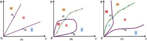
When $\delta >1$, the enhancing domain is Domain II ∪ IV, which is bounded, while the attracting domain of $E_2^{\ast }$ is Domain (I+II), see Figure 1(b). Hence, any solution to (4(4) $\frac{\mathrm{d}x}{\mathrm{d}t}=\beta (1-\mu )x-\delta x(x+y):=f(x,y),$(4) ) and (5(5) $\frac{\mathrm{d}y}{\mathrm{d}t}=\beta \mu x+\frac{y^2}{x+y}-y(x+y):=g(x,y),$(5) ) initiated from Domain I approaches to $E_2^{\ast }$, but $p\left(t\right)$ does not always increase. And any solution initiated from Domain IV approaches to Wolbachia-free equilibrium point $E_1(0,1)$, but $p\left(t\right)$ does not always decrease.

When $\delta <1$, the enhancing domain is Domain (II+III), which is unbounded, while the attracting domain of $E_2^{\ast }$ is Domain (I+II+V), see Figure 1(c). Hence, any solution to (4(4) $\frac{\mathrm{d}x}{\mathrm{d}t}=\beta (1-\mu )x-\delta x(x+y):=f(x,y),$(4) ) and (5(5) $\frac{\mathrm{d}y}{\mathrm{d}t}=\beta \mu x+\frac{y^2}{x+y}-y(x+y):=g(x,y),$(5) ) initiated from Domain I or Domain V approaches to $E_2^{\ast }$, but $p\left(t\right)$ does not always increase. And any solution initiated from Domain IV approaches to Wolbachia-free equilibrium point $E_1(0,1)$, but $p\left(t\right)$ does not always decrease.

The gap between $E^I$ and $A^I$ suggests that the design or adjustment of releasing strategies could not be based solely on the surveillance of the infection frequency. To see what does the conclusion imply biologically that may be instructive to the design of release strategies, we take the benign Wolbachia strain, wMel, of A. aegypti as an example since wMel infected mosquitoes are currently being deployed in several countries for the control of arboviruses [34]. The findings in [33] shows that wMel brings no significant fecundity cost to the host, and causes only 10% longevity reduction. Based on the laboratory data in [33], from the oviposition rate, egg hatching rate, the survival rate of larvae to adults we estimated the birth rates $b_I$ and $b_U$ as $b_I=0.3976,b_U=\mathrm{0.3976.}$ The decay rates ${\delta }_I$ and ${\delta }_U$ are estimated from the half-life of adults as ${\delta }_I=9.4482\times {10}^{-6},{\delta }_U=8.5034\times {10}^{-6}.$ Hence, from the rescaling (3(3) $x=\frac{2{\delta }_U}{b_U}I,y=\frac{2{\delta }_U}{b_U}U,s=\frac{b_U}{2}t,\beta =\frac{b_I}{b_U},\delta =\frac{{\delta }_I}{{\delta }_U},$(3) ) we have $\beta =\frac{0.3976}{0.3976}=1,\delta =\frac{9.4482\times {10}^{-6}}{8.5034\times {10}^{-6}}\approx \mathrm{1.1111.}$ We take $\mu =0.05$ to account for the maternal leakage of infected mothers [26]. Under these parameters, system (4(4) $\frac{\mathrm{d}x}{\mathrm{d}t}=\beta (1-\mu )x-\delta x(x+y):=f(x,y),$(4) ) and (5(5) $\frac{\mathrm{d}y}{\mathrm{d}t}=\beta \mu x+\frac{y^2}{x+y}-y(x+y):=g(x,y),$(5) ) admits two interior equilibria $E_1^{\ast }=(0.1318,0.7233),E_2^{\ast }=(0.8045,0.0505).$$E_1^{\ast }$ is a saddle point, and $E_2^{\ast }$ is an asymptotically stable polymorphic point [40], which denotes the coexistence of infected and uninfected mosquitoes with infection frequency $\frac{0.8045}{0.8045+0.0505}\approx 0.9409:=p^{\mathrm{stable}}.$ 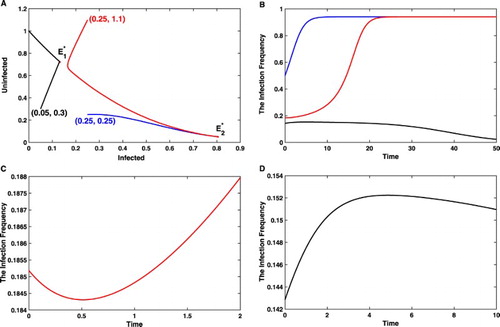To proceed, we take three special initial values: $(0.25,0.25)$, $(0.25,1.1)$, and $(0.05,0.3).$ The corresponding solutions to (4(4) $\frac{\mathrm{d}x}{\mathrm{d}t}=\beta (1-\mu )x-\delta x(x+y):=f(x,y),$(4) ) and (5(5) $\frac{\mathrm{d}y}{\mathrm{d}t}=\beta \mu x+\frac{y^2}{x+y}-y(x+y):=g(x,y),$(5) ) are shown in Figure 2(a), which shows that $(0.25,0.25)\in A^I,(0.25,1.1)\in A^I,\mathrm{and}(0.05,0.3)\notin A^I.$ Further simulations manifest the oscillation behaviour of the infection frequency $p=x/(x+y)$ against time t, see Figure 2(b). Although both solutions initialized at $(0.25,1.1)$ and $(0.25,0.25)$ make Wolbachia infection goes to fixation at polymorphic state, there is a great discrepancy on the dynamics of the infection frequency. Initiated from $(0.25,0.25)$, the infection frequency monotonically increases to $p^{\mathrm{stable}}$. In contrast, p decreases first before it climbs up to $p^{\mathrm{stable}}$ when initialized from $(0.25,1.1)$, see Figure 2(c). In contrast, although the infection frequency goes to 0 when initialized from $(0.05,0.3)$, it has a short time period during which the infection frequency increases first and then decreases to 0, see Figure 2(d).

Figure 2. The deceptive phenomena based solely on the infection frequency. (a) Starting from $(0.25,0.25)$ or $(0.25,1.1)$, the infected and uninfected mosquitoes eventually go to a polymorphic state, while the initial population size $(0.05,0.3)$ results in Wolbachia extinction. (b) The blue curve sketches the infection frequency p against t with the initial population size $(0.25,0.25)$, and the red and black curves are for initial population sizes $(0.25,1.1)$ and $(0.05,0.3)$, respectively. (c) Initiated from the population size $(0.25,1.1)$, corresponding to the initial infection frequency $\approx 0.1852;$, the infection frequency decreases before it goes to the stable polymorphic frequency $\approx 0.9409;$. (d) Initiated from the population size $(0.05,0.3)$, corresponding to the initial infection frequency $\approx 0.1429;$, the infection frequency increases before it goes to 0. Both (c) and (d) show that before Wolbachia goes to fixation or extinction, it is possible for the infection frequency to oscillate, which implies that we need to monitor $p\left(t\right)$ continuously to inform whether or not extra releases should be contemplated.

Compared to estimating the absolute population sizes of infected and uninfected mosquitoes, a more direct and plausible method is to monitor whether the more measurable quantity $p\left(t\right)$ is going up or down. However, our observations imply that when designing release strategies, one should take both the initial population size and the infection frequency into account. Decision made solely from the growth of the infection frequency could be inaccurate and misleading: The success of Wolbachia fixation permits the transient decrease of the infection frequency, and the short-time period of increase of the infection frequency is not always sufficient for the success of Wolbachia fixation.

Acknowledgements

We are grateful to the three reviewers' valuable and precious suggestions.

Disclosure statement

No potential conflict of interest was reported by the authors.

Additional information

Funding

This work was supported by Department of Education of Guangdong Province [2017KTSCX148], National Natural Science Foundation of China [11631005, 11626246], Program for Changjiang Scholars and Innovative Research Team in University [IRT_16R16], and Scientific and Technological Leading Talents of Guangzhou Development District [2013L-P116].

References

- C.M. Atyame, J. Cattel, C. Lebon, O. Flores, J.S. Dehecq, M. Weill, L.C. Gouagna and P. Tortosa, Wolbachia-based population control strategy targeting Culex quinquefasciatus mosquitoes proves efficient under semi-field conditions, PLoS One 10(3) (2015), e0119288. doi: 10.1371/journal.pone.0119288
- G. Bian, Y. Xu, P. Lu and Z. Xi, The endosymbiotic bacterium Wolbachia induces resistance to dengue virus in Aedes aegypti, PLoS Pathog. 6(4) (2010), e1000833. doi: 10.1371/journal.ppat.1000833
- G. Bian, D. Joshi, Y. Dong, P. Lu, G. Zhou, X. Pan, Y. Xu, G. Dimopoulos and Z. Xi, Wolbachia invades Anopheles stephensi populations and induces refractoriness to plasmodium infection, Science 340 (2013), pp. 748–751. doi: 10.1126/science.1236192
- L. Cai, S. Ai and J. Li, Dynamics of mosquitoes populations with different strategies for releasing sterile mosquitoes, SIAM J. Appl. Math. 74(6) (2014), pp. 1786–1809. doi: 10.1137/13094102X
- L.B. Carrington, J.R. Lipkowitz, A.A. Hoffmann and M. Turelli, A re-examination of Wolbachia-induced cytoplasmic incompatibility in California Drosophila simulans, PLoS One 6(7) (2011), e22565. doi: 10.1371/journal.pone.0022565
- M.H.T Chan and P.S. Kim, Modelling a Wolbachia invasion using a slow-fast dispersal reaction-diffusion approach, Bull. Math. Biol. 75(9) (2013), pp. 1501–1523. doi: 10.1007/s11538-013-9857-y
- H.L. Dutra, L.M. Dos Santos, E.P. Caragata, J.B. Silva, D.A. Villela and R. Maciel-De-Freitas, From lab to field: the influence of urban landscapes on the invasive potential of Wolbachia in Brazilian Aedes aegypti mosquitoes, PLoS Negl. Trop. Dis. 9(4) (2015), pp. 1–22. doi: 10.1371/journal.pntd.0003689
- F.D. Frentiu, T. Zakir, T. Walker, J. Popovici, A.T. Pyke and D.H.A Van, Limited dengue virus replication in field-collected Aedes aegypti mosquitoes infected with Wolbachia, PLoS Neglected Tropical Diseases 8(2) (2014), pp. 793–800. doi: 10.1371/journal.pntd.0002688
- A.A. Hoffmann and M. Turelli, Unidirectional incompatibility in Drosophila simulans: inheritance, geographic variation and fitness effects, Genetics 119(2) (1988), pp. 435–444.
- A.A. Hoffmann, B.L. Montgomery, J. Popovici, I. Iturbeormaetxe, P.H. Johnson, F. Muzzi, M. Greenfield, M. Durkan, Y.S. Leong, Y. Dong, H. Cook, J. Axford, A.G. Gallahan, N. Kenny, C. Omodei, E.A. McGraw, P.A. Ryan, S.A. Ritchie, M. Turelli and S.L. O'Neill, Successful establishment of Wolbachia in Aedes populations to suppress dengue transmission, Nature 476(7361) (2011), pp. 454–459. doi: 10.1038/nature10356
- A.A. Hoffmann, I. Iturbeormaetxe, A.G. Callahan, B.L. Phillips, K. Billington, J.K. Axford, B. Montgomery, A.P. Turley and S.L. O'Neill, Stability of the wMel Wolbachia infection following Invasion into Aedes aegypti populations, PLoS Neglect Trop D 8(9) (2014), e3115. doi: 10.1371/journal.pntd.0003115
- L. Hu, M. Huang, M. Tang, J. Yu and B. Zheng, Wolbachia spread dynamics in stochastic environments, Theor. Popul. Biol. 106 (2015), pp. 32–44. doi: 10.1016/j.tpb.2015.09.003
- M. Huang, M. Tang and J. Yu, Wolbachia infection dynamics by reaction-diffusion equations, Sci. China Math. 58(1) (2015), pp. 77–96. doi: 10.1007/s11425-014-4934-8
- M. Huang, J. Yu, L. Hu and B. Zheng, Qualitative analysis for a Wolbachia infection model with diffusion, Sci. China Math. 59(7) (2016), pp. 1249–1266. doi: 10.1007/s11425-016-5149-y
- M. Huang, J. Luo, L. Hu, B. Zheng and J. Yu, Assessing the efficiency of Wolbachia driven Aedes mosquito suppression by delay differential equations, J. Theor. Biol. 440 (2018), pp. 1–11. doi: 10.1016/j.jtbi.2017.12.012
- M.J. Keeling, F.M. Jiggins and J.M. Read, The invasion and coexistence of competing Wolbachia strains, Heredity 91(4) (2003), pp. 382–388. doi: 10.1038/sj.hdy.6800343
- P. Kriesner, A.A. Hoffmann, S.F. Lee, M. Turelli and A.R. Weeks, Rapid sequential spread of two Wolbachia variants in Drosophila simulans, PLoS Pathogens 9(9) (2013), pp. 289–290. doi: 10.1371/journal.ppat.1003607
- P. Kriesner, W.R. Conner, A.R. Weeks, M. Turelli and A.A. Hoffmann, Persistence of a Wolbachia infection frequency cline in Drosophila melanogaster and the possible role of reproductive dormancy, Evolution 70(5) (2016), pp. 979–997. doi: 10.1111/evo.12923
- J. Li, New revised simple models for interactive wild and sterile mosquito populations and their dynamics, J. Biol. Dyn. 11(S2) (2017), pp. 316–333. doi: 10.1080/17513758.2016.1216613
- J. Li and Z. Yuan, Modelling releases of sterile mosquitoes with different strategies, J. Biol. Dyn. 9(1) (2015), pp. 1–14. doi: 10.1080/17513758.2014.977971
- L.A. Moreira, I. Iturbeormaetxe, J.A. Jeffery, G. Lu, A.T. Pyke, L.M. Hedges, B.C. Rocha, S. Hall-Mendelin, A. Day, M. Riegler, L.E. Hugo, K.N. Johnson, B.H. Kay, E.A. McGraw, A.F. Van den Hurk, P.A. Ryan and S.L. O'Neill, A Wolbachia symbiont in Aedes aegypti limits infection with dengue, Chikungunya, and Plasmodium, Cell 139(7) (2009), p. 1268. doi: 10.1016/j.cell.2009.11.042
- M.A. Ndii, R.I. Hickson and G.N. Mercer, Modelling the introduction of Wolbachia into Aedes aegypti mosquitoes to reduce dengue transmission, ANZIAM Journal 53(3) (2012), pp. 213–227. doi: 10.1017/S1446181112000132
- T.H. Nguyen, H.L. Nguyen, T.Y. Nguyen, S.N. Vu, N.D. Tran, T.N. Le, S. Kutcher, T.P. Hurst, T.T. Duong, J.A. Jeffery, J.M. Darbro, B.H. Kay, I. Iturbe-Ormaetxe, J. Popovici, B.L. Montgomery, A.P. Turley, F. Zigterman, H. Cook, P.E. Cook, P.H. Johnson, P.A. Ryan, C.J. Paton, S.A. Ritchie, C.P. Simmons, S.L. O'Neill and A.A. Hoffmann, Field evaluation of the establishment potential of wMelPop Wolbachia in Australia and Vietnam for dengue control, Parasites Vectors 8(1) (2015), pp. 1–14. doi: 10.1186/s13071-015-1174-x
- L. O'Connor, C. Plichart, A.C. Sang, C.L. Brelsfoard, H.C. Bossin and S.L. Dobson, Open release of male mosquitoes infected with a Wolbachia biopesticide: field performance and infection containment, PLoS Negl. Trop. D 6(11) (2012), pp. e1797. doi: 10.1371/journal.pntd.0001797
- S.A. Ritchie, A.F.V.D. Hurk, M.J. Smout, K.M. Staunton and A.A. Hoffmann, Mission accomplished? We need a guide to the ‘Post Release’ world of Wolbachia for Aedes-borne disease control, Trends Parasitol. 34(3) (2018), pp. 217–226. doi: 10.1016/j.pt.2017.11.011
- P.A. Ross, I. Wiwatanaratanabutr, J.K. Axford, V.L. White, N.M. Endersby-Harshman and A.A. Hoffmann, Wolbachia infections in Aedes aegypti differ markedly in their response to cyclical heat stress, PLoS Pathog. 13(1) (2017), pp. e1006006. doi: 10.1371/journal.ppat.1006006
- T.L. Schmidt, I. Filipović, A.A. Hoffmann and G. Rašić, Fine-scale landscape genomics helps explain the slow spatial spread of Wolbachia through the Aedes aegypti population in Cairns, Australia, Heredity 120 (2018), pp. 386–395. doi: 10.1038/s41437-017-0039-9
- B. Tang, Y. Xiao, S. Tang and J. Wu, Modelling weekly vector control against Dengue in the Guangdong Province of China, J. Theor. Biol. 410 (2016), pp. 65–76. doi: 10.1016/j.jtbi.2016.09.012
- M. Turelli, Cytoplasmic incompatibility in populations with overlapping generations, Evolution 64 (2010), pp. 232–241. doi: 10.1111/j.1558-5646.2009.00822.x
- M. Turelli and N.H. Barton, Deploying dengue-suppressing Wolbachia: Robust models predict slow but effective spatial spread in Aedes aegypti, Theor. Popul. Biol. 115 (2017), pp. 45–60. doi: 10.1016/j.tpb.2017.03.003
- M. Turelli and A.A. Hoffmann, Rapid spread of an inherited incompatibility factor in California Drosophila, Nature 353 (1991), pp. 440–442. doi: 10.1038/353440a0
- M. Turelli and A.A. Hoffmann, Cytoplasmic incompatibility in Drosophila simulans: dynamics and parameter estimates from natural populations, Genetics 140 (1991), pp. 1319–1338.
- T. Walker, P.H. Johnson, L.A. Moreira, I. Iturbeormaetxe, F.D. Frentiu, C.J. McMeniman, Y.S. Leong, Y. Dong, J. Axford, P. Kriesner, A.L. Lloyd, S.A. Ritchie, S.L. O'Neill and A.A. Hoffmann, The wMel Wolbachia strain blocks dengue and invades caged Aedes aegypti populations, Nature 476(7361) (2011), pp. 450–453. doi: 10.1038/nature10355
- World Mosquito Program: Country Projects, 2018. Available at http://www.eliminatedengue.com/program.
- Z. Xi, J.L. Dean, C.C. Khoo and S.L. Dobson, Generation of a novel Wolbachia infection in Aedes albopictus (Asian tiger mosquito) via embryonic microinjection, Insect Biochem. Molec. Biol. 35(8) (2005), pp. 903–910. doi: 10.1016/j.ibmb.2005.03.015
- Z. Xi, C.C. Khoo and S.L. Dobson, Wolbachia establishment and invasion in an Aedes aegypti laboratory population, Science 310(5746) (2005), pp. 326–328. doi: 10.1126/science.1117607
- X. Zhang, S. Tang and R.A. Cheke, Models to assess how best to replace dengue virus vectors with Wolbachia-infected mosquito populations, Math. Biosci. 269 (2015), pp. 164–177. doi: 10.1016/j.mbs.2015.09.004
- X. Zhang, S. Tang, Q. Liu, R.A. Cheke and H. Zhu, Models to assess the effects of non-identical sex ratio augmentations of Wolbachia-carrying mosquitoes on the control of dengue disease, Math. Biosci. 299 (2018), pp. 58–72. doi: 10.1016/j.mbs.2018.03.003
- B. Zheng, M. Tang and J. Yu, Modeling Wolbachia spread in mosquitoes through delay differential equations, SIAM J. Appl. Math. 74(3) (2014), pp. 743–770. doi: 10.1137/13093354X
- B. Zheng, M. Tang, J. Yu and J. Qiu, Wolbachia spreading dynamics in mosquitoes with imperfect maternal transmission, J. Math. Biol. 76(1–2) (2018), pp. 235–263. doi: 10.1007/s00285-017-1142-5
- B. Zheng, W. Guo, L. Hu and J. Yu, Complex Wolbachia infection dynamics in mosquitoes with imperfect maternal transmission, Math. Biosci. Eng. 15(2) (2018), pp. 523–541. doi: 10.3934/mbe.2018024