Theoretical and numerical results for an age-structured SIVS model with a general nonlinear incidence rate

ABSTRACT

In this paper, we propose an SIVS epidemic model with continuous age structures in both infected and vaccinated classes and with a general nonlinear incidence. Firstly, we provide some basic properties of the system including the existence, uniqueness and positivity of solutions. Furthermore, we show that the solution semiflow is asymptotic smooth. Secondly, we calculate the basic reproduction number ${\mathcal{R}}_0$ by employing the classical renewal process, which determines whether the disease persists or not. In the main part, we investigate the global stability of the equilibria by the approach of Lyanpunov functionals. Some numerical simulations are conducted to illustrate the theoretical results and to show the effect of the transmission rate and immunity waning rate on the disease prevalence.

KEYWORDS:

• Infection age
• vaccination age
• nonlinear incidence
• persistence
• Lyapunov functional

1. Introduction

Vaccination is one of the most effective methods of preventing infectious diseases. Indeed, for some children diseases like Measles, Rubella, and Chicken pox, preventive vaccines may provide a permanent immunity against the diseases. However, life-long immunity cannot be offered by preventive vaccines for some diseases such as Hepatitis B, Influenza, and Mumps. The immunity of vaccinated persons will wane and they will become vulnerable to the diseases again. It is necessary to design a framework to study the effect of waning immunity on the spread of an epidemic. Compartmental models have been developed to provide deep insights on the dynamics of an epidemic with non-permanent immunity (see, for example, [5,19,29]).

It is strongly supported by data that a vaccine usually wanes with respect to the vaccinated time. Many scholars have successfully addressed this by adding a vaccinated compartment to classic epidemic models [6,10,15,18,30,31]. Obtained results include threshold dynamics [6,30,31] and backward bifurcation [18]. In this regard, the immunity duration has been becoming an important issue for the evolution and efficacy of the vaccine. Recently, we proposed an SIVS-type epidemic model with vaccination age in [31] to explore the non-fixed immunity duration, (1) $\begin{array}{rl}& \frac{\mathrm{d}S\left(t\right)}{\mathrm{d}t}=\mathrm{\Lambda }-\mu S\left(t\right)-S\left(t\right)f\left(I\right(t\left)\right)-\phi S\left(t\right)+{\int }_0^{\mathrm{\infty }}\epsilon \left(a\right)v(t,a)\mathrm{d}a,\\ & \frac{dI\left(t\right)}{dt}=S\left(t\right)f\left(I\right(t\left)\right)-(\mu +\gamma +\delta )I\left(t\right),\\ & \frac{\mathrm{\partial }v(t,a)}{\mathrm{\partial }t}+\frac{\mathrm{\partial }v(t,a)}{\mathrm{\partial }a}=-(\mu +\epsilon (a\left)\right)v(t,a),\\ & v(t,0)=\phi S\left(t\right),\\ & S\left(0\right)=S_0\ge 0,I\left(0\right)=I_0>0,v(0,\cdot )=v_0(\cdot )\in L_{+}^1\triangleq L^1({\mathbb{R}}_{+};{\mathbb{R}}_{+}),\end{array}$(1) where $S\left(t\right)$ and $I\left(t\right)$ denote the population sizes of the susceptible and infected at time t, respectively; $v(t,a)$ denotes the population density of the vaccinated at time t with vaccination age a. The parameters have the following meanings: Λ is the input rate of the new members, μ denotes the natural death rate, φ represents the vaccinated rate for the susceptible, γ denotes the cure rate for infected individuals, δ represents the disease-caused death rate of infected individuals, $\epsilon \left(a\right)$ denotes the immunity waning rate at age a, $f\left(I\right)$ represents the incidence rate and satisfies the following property: $f\left(0\right)=0,f^{\prime }\left(I\right)>0,f^{″}\left(I\right)<0.$ We showed that system (1(1) $\begin{array}{rl}& \frac{\mathrm{d}S\left(t\right)}{\mathrm{d}t}=\mathrm{\Lambda }-\mu S\left(t\right)-S\left(t\right)f\left(I\right(t\left)\right)-\phi S\left(t\right)+{\int }_0^{\mathrm{\infty }}\epsilon \left(a\right)v(t,a)\mathrm{d}a,\\ & \frac{dI\left(t\right)}{dt}=S\left(t\right)f\left(I\right(t\left)\right)-(\mu +\gamma +\delta )I\left(t\right),\\ & \frac{\mathrm{\partial }v(t,a)}{\mathrm{\partial }t}+\frac{\mathrm{\partial }v(t,a)}{\mathrm{\partial }a}=-(\mu +\epsilon (a\left)\right)v(t,a),\\ & v(t,0)=\phi S\left(t\right),\\ & S\left(0\right)=S_0\ge 0,I\left(0\right)=I_0>0,v(0,\cdot )=v_0(\cdot )\in L_{+}^1\triangleq L^1({\mathbb{R}}_{+};{\mathbb{R}}_{+}),\end{array}$(1) ) exhibits a threshold dynamics by constructing appropriate Lyapunov functionals. In this sense, the basic reproduction number ${\mathcal{R}}_0$ is a key value determining whether the disease dies out or persists.

As we know, the incidence rate is an important factor affecting the disease dynamics. In the above mentioned works, the incidences used include the bilinear-type ($\beta SI$) [5,6,18,19], the standard-type ($\beta SI/(S+I)$) [15], the saturated-type $Sf\left(I\right)$ [30,31], and the nonlinear-type $S^p{I}^q$ [29]. In the literature, Feng and Thieme firstly proposed a nonlinear general incidence of the form $f(S,I)$ [8]. Thereafter, Huang et al. [13] and Korobeinikov [17] studied some epidemic models with incidence rates of the form $f\left(S\right)g\left(I\right)$. Furthermore, Korobeinikov [16] obtained the global stability of basic SIR and SIRS epidemic models with the incidence rate of the form $f(S,I)$.

Most classical epidemic models are compartmental models described by ordinary differential equations, where all infectious individuals are assumed to be homogeneous during their infectious period. This assumption has been proved to be reasonable in the study of the dynamics of communicable diseases such as influenza as well as in the study of sexually transmitted diseases. However, infectivity experiments on HIV/AIDS indicate that the transmission style follows an early infectivity peak (a few weeks after exposure) and a late infectivity plateau [9]. To describe such a phenomenon, the concept of infection age (the time that has passed since infection) has been introduced into classical models. Therefore, epidemic models with infection age have been extensively studied in the literature. To name a few, see [3,4,22,25,28,32], where the incidence is bilinear in most of the models. Recently, epidemic models with infection age and nonlinear incidence have been extensively studied (see, for instance, [4,25,28]).

To the best of our knowledge, not much has been done for epidemic models with two age structures [7,23]. In [23], McCluskey considered an SEI model with continuous age structures in both the exposed and infectious classes and a threshold dynamics was established by using the approach of Lyapunov functionals while in [7], Duan et al. studied an SVEIR epidemic model with ages of vaccination and latency and also obtained a threshold dynamics. Magal and McCluskey in [21] proposed a two group SI epidemic model with age of infection and discussed the global stability of steady states.

Motivated by the above discussion, the purpose of this paper is to make further contribution to the study of epidemic models with two age structures and nonlinear incidence. Precisely, we introduce age structure into the infected individuals in (1(1) $\begin{array}{rl}& \frac{\mathrm{d}S\left(t\right)}{\mathrm{d}t}=\mathrm{\Lambda }-\mu S\left(t\right)-S\left(t\right)f\left(I\right(t\left)\right)-\phi S\left(t\right)+{\int }_0^{\mathrm{\infty }}\epsilon \left(a\right)v(t,a)\mathrm{d}a,\\ & \frac{dI\left(t\right)}{dt}=S\left(t\right)f\left(I\right(t\left)\right)-(\mu +\gamma +\delta )I\left(t\right),\\ & \frac{\mathrm{\partial }v(t,a)}{\mathrm{\partial }t}+\frac{\mathrm{\partial }v(t,a)}{\mathrm{\partial }a}=-(\mu +\epsilon (a\left)\right)v(t,a),\\ & v(t,0)=\phi S\left(t\right),\\ & S\left(0\right)=S_0\ge 0,I\left(0\right)=I_0>0,v(0,\cdot )=v_0(\cdot )\in L_{+}^1\triangleq L^1({\mathbb{R}}_{+};{\mathbb{R}}_{+}),\end{array}$(1) ) and use a general incidence. Furthermore, let $i(t,a)$ denote the density of infected individuals at time t with infection age a. The model to be studied is as follows, (2) $\begin{array}{rl}& \frac{\mathrm{d}S\left(t\right)}{\mathrm{d}t}=\mathrm{\Lambda }-\mu S\left(t\right)-f\left(S\right(t),J(t\left)\right)-\phi S\left(t\right)+{\int }_0^{\mathrm{\infty }}\epsilon \left(a\right)v(t,a)\mathrm{d}a,\\ & \frac{\mathrm{\partial }i(t,a)}{\mathrm{\partial }t}+\frac{\mathrm{\partial }i(t,a)}{\mathrm{\partial }a}=-(\mu +\gamma (a)+\delta (a\left)\right)i(t,a),\\ & i(t,0)=f\left(S\right(t),J(t\left)\right),J\left(t\right)={\int }_0^{\mathrm{\infty }}\beta \left(a\right)i(t,a)\mathrm{d}a,\\ & \frac{\mathrm{\partial }v(t,a)}{\mathrm{\partial }t}+\frac{\mathrm{\partial }v(t,a)}{\mathrm{\partial }a}=-(\mu +\epsilon (a\left)\right)v(t,a),\\ & v(t,0)=\phi S\left(t\right),\end{array}$(2) with initial condition $S\left(0\right)=S_0\ge 0,i(0,\cdot )=i_0(\cdot )\in L_{+}^1,v(0,\cdot )=v_0(\cdot )\in L_{+}^1.$ Here Λ, μ, φ, and $\epsilon \left(a\right)$ have the same biological meanings as in those (1(1) $\begin{array}{rl}& \frac{\mathrm{d}S\left(t\right)}{\mathrm{d}t}=\mathrm{\Lambda }-\mu S\left(t\right)-S\left(t\right)f\left(I\right(t\left)\right)-\phi S\left(t\right)+{\int }_0^{\mathrm{\infty }}\epsilon \left(a\right)v(t,a)\mathrm{d}a,\\ & \frac{dI\left(t\right)}{dt}=S\left(t\right)f\left(I\right(t\left)\right)-(\mu +\gamma +\delta )I\left(t\right),\\ & \frac{\mathrm{\partial }v(t,a)}{\mathrm{\partial }t}+\frac{\mathrm{\partial }v(t,a)}{\mathrm{\partial }a}=-(\mu +\epsilon (a\left)\right)v(t,a),\\ & v(t,0)=\phi S\left(t\right),\\ & S\left(0\right)=S_0\ge 0,I\left(0\right)=I_0>0,v(0,\cdot )=v_0(\cdot )\in L_{+}^1\triangleq L^1({\mathbb{R}}_{+};{\mathbb{R}}_{+}),\end{array}$(1) ). For the other parameters, $\gamma \left(a\right)$ is the recovery rate of the infected with infection age a, $\delta \left(a\right)$ is the disease-induced death rate with infection age a, and $\beta \left(a\right)$ is the transmission coefficient with infection age a. In epidemiology, $J\left(t\right)$ is called the force of infection, which justifies the form of incidence $f\left(S\right(t),J(t\left)\right)$. Note that the models in [4,6,7,22,31] are just special cases of (2(2) $\begin{array}{rl}& \frac{\mathrm{d}S\left(t\right)}{\mathrm{d}t}=\mathrm{\Lambda }-\mu S\left(t\right)-f\left(S\right(t),J(t\left)\right)-\phi S\left(t\right)+{\int }_0^{\mathrm{\infty }}\epsilon \left(a\right)v(t,a)\mathrm{d}a,\\ & \frac{\mathrm{\partial }i(t,a)}{\mathrm{\partial }t}+\frac{\mathrm{\partial }i(t,a)}{\mathrm{\partial }a}=-(\mu +\gamma (a)+\delta (a\left)\right)i(t,a),\\ & i(t,0)=f\left(S\right(t),J(t\left)\right),J\left(t\right)={\int }_0^{\mathrm{\infty }}\beta \left(a\right)i(t,a)\mathrm{d}a,\\ & \frac{\mathrm{\partial }v(t,a)}{\mathrm{\partial }t}+\frac{\mathrm{\partial }v(t,a)}{\mathrm{\partial }a}=-(\mu +\epsilon (a\left)\right)v(t,a),\\ & v(t,0)=\phi S\left(t\right),\end{array}$(2) ) and hence over results will cover those in the above-mentioned references.

Throughout this paper, we make the following assumptions on the parameter functions.

(A1)	The functions ϵ, $\beta \in C_{BU}({\mathbb{R}}_{+},{\mathbb{R}}_{+})$, where $C_{BU}({\mathbb{R}}_{+},{\mathbb{R}}_{+})$ is the set of all bounded and uniformly continuous functions from ${\mathbb{R}}_{+}$ to ${\mathbb{R}}_{+}$.
(A2)	The functions γ, $\delta \in L_{+}^{\mathrm{\infty }}\left({\mathbb{R}}_{+}\right)$, the nonnegative cone of $L^{\mathrm{\infty }}\left({\mathbb{R}}_{+}\right)$.

Moreover, we suppose that the nonlinear incidence f satisfies:

(B1)	For S, $J\in {\mathbb{R}}^{+}$, $f(0,J)=f(S,0)=0$; $\mathrm{\partial }f(S,J)/\mathrm{\partial }S>0$ for J>0; $\mathrm{\partial }f(S,J)/\mathrm{\partial }J>0$ for S>0; and $\mathrm{\partial }{f}^2(S,J)/\mathrm{\partial }{J}^2\le 0$.

Assumption (B1) is a combination of those in [17,25]. It is easy to see that f is locally Lipschitz continuous on S and J, that is, for every C>0, there exists some $L:=L_C>0$ such that (3) $\parallel f(S_1,J_1)-f(S_2,J_2)\parallel \le L(|S_1-S_2|+|J_1-J_2|),$(3) whenever $0\le S_1$, $S_2$, $J_1$, $J_2\le C$.

The pahse space of (2(2) $\begin{array}{rl}& \frac{\mathrm{d}S\left(t\right)}{\mathrm{d}t}=\mathrm{\Lambda }-\mu S\left(t\right)-f\left(S\right(t),J(t\left)\right)-\phi S\left(t\right)+{\int }_0^{\mathrm{\infty }}\epsilon \left(a\right)v(t,a)\mathrm{d}a,\\ & \frac{\mathrm{\partial }i(t,a)}{\mathrm{\partial }t}+\frac{\mathrm{\partial }i(t,a)}{\mathrm{\partial }a}=-(\mu +\gamma (a)+\delta (a\left)\right)i(t,a),\\ & i(t,0)=f\left(S\right(t),J(t\left)\right),J\left(t\right)={\int }_0^{\mathrm{\infty }}\beta \left(a\right)i(t,a)\mathrm{d}a,\\ & \frac{\mathrm{\partial }v(t,a)}{\mathrm{\partial }t}+\frac{\mathrm{\partial }v(t,a)}{\mathrm{\partial }a}=-(\mu +\epsilon (a\left)\right)v(t,a),\\ & v(t,0)=\phi S\left(t\right),\end{array}$(2) ) is $X={\mathbb{R}}_{+}\times L_{+}^1\times L_{+}^1$. For $(S_0,i_0,v_0)\in X$, we denote $\parallel (S_0,i_0,v_0){\parallel }_X=S_0+\parallel i_0{\parallel }_1+\parallel v_0{\parallel }_1.$ In order to study the existence of solutions to (2(2) $\begin{array}{rl}& \frac{\mathrm{d}S\left(t\right)}{\mathrm{d}t}=\mathrm{\Lambda }-\mu S\left(t\right)-f\left(S\right(t),J(t\left)\right)-\phi S\left(t\right)+{\int }_0^{\mathrm{\infty }}\epsilon \left(a\right)v(t,a)\mathrm{d}a,\\ & \frac{\mathrm{\partial }i(t,a)}{\mathrm{\partial }t}+\frac{\mathrm{\partial }i(t,a)}{\mathrm{\partial }a}=-(\mu +\gamma (a)+\delta (a\left)\right)i(t,a),\\ & i(t,0)=f\left(S\right(t),J(t\left)\right),J\left(t\right)={\int }_0^{\mathrm{\infty }}\beta \left(a\right)i(t,a)\mathrm{d}a,\\ & \frac{\mathrm{\partial }v(t,a)}{\mathrm{\partial }t}+\frac{\mathrm{\partial }v(t,a)}{\mathrm{\partial }a}=-(\mu +\epsilon (a\left)\right)v(t,a),\\ & v(t,0)=\phi S\left(t\right),\end{array}$(2) ), we will extend X.

Let $Y=\mathbb{R}\times L^1({\mathbb{R}}_{+};\mathbb{R})$, $Y_0=\left\{0\right\}\times L^1({\mathbb{R}}_{+};\mathbb{R})$, $Y_{+}={\mathbb{R}}_{+}\times L_{+}^1$, and $Y_{+0}=Y_{+}\bigcap Y_0$. Define two linear operators $A_j:D\left(A_j\right)\subset Y\to Y$ (j=1, 2) as follows. (4) $\begin{array}{l}{A}_1\left(\begin{array}{c}0\\ {\phi }_1\end{array}\right)=\left(\begin{array}{c}-{\phi }_1\left(0\right)\\ -{\phi }_1^{\prime }-(\mu +\gamma (a)+\delta (a\left)\right){\phi }_1\end{array}\right),\\ D\left(A_1\right)=\left\{\left(\begin{array}{c}0\\ {\phi }_1\end{array}\right)\in Y|\phi \text{ is absolutely continuous and}{\phi }_1^{\prime }\in L^1({\mathbb{R}}_{+};\mathbb{R})\right\},\end{array}$(4) and (5) $\begin{array}{l}{A}_2\left(\begin{array}{c}0\\ {\phi }_2\end{array}\right)=\left(\begin{array}{c}-{\phi }_2\left(0\right)\\ -{\phi }_2^{\prime }-(\mu +\epsilon (a\left)\right){\phi }_2\end{array}\right),\\ D\left(A_2\right)=\left\{\left(\begin{array}{c}0\\ {\phi }_2\end{array}\right)\in Y|{\phi }_2\text{ is absolutely continuous and}{\phi }_2^{\prime }\in L^1({\mathbb{R}}_{+};\mathbb{R})\right\}.\end{array}$(5) For any $\lambda \in \rho \left(A_1\right)$ ($\rho \left(A_1\right)$ denotes the resolvent set of $A_1$) and $\left(\begin{array}{c}0\\ {\phi }_1\end{array}\right)\in D\left(A_1\right)$, if $(\lambda I-A_1{)}^{-1}\left(\begin{array}{c}{\alpha }_1\\ {\theta }_1\end{array}\right)=\left(\begin{array}{c}0\\ {\phi }_1\end{array}\right),\left(\begin{array}{c}{\alpha }_1\\ {\theta }_1\end{array}\right)\in Y,$ then by simple calculation we obtain (6) ${\phi }_1\left(a\right)={\alpha }_1{\mathrm{e}}^{-(\lambda +\mu )a-{\int }_0^a\left(\gamma \right(\xi )+\delta (\xi \left)\right)\mathrm{d}\xi }+{\int }_0^a{\theta }_1\left(s\right){\mathrm{e}}^{-(\lambda +\mu )(a-s)}{\mathrm{e}}^{-{\int }_s^a\left(\gamma \right(\xi )+\delta (\xi \left)\right)\mathrm{d}\xi }\mathrm{d}s.$(6) Similarly, for any $\lambda \in \rho \left(A_2\right)$ and $\left(\begin{array}{c}0\\ {\phi }_2\end{array}\right)\in D\left(A_2\right)$, if $(\lambda -A_2{)}^{-1}\left(\begin{array}{c}{\alpha }_2\\ {\theta }_2\end{array}\right)=\left(\begin{array}{c}0\\ {\phi }_2\end{array}\right)$ with $\left(\begin{array}{c}{\alpha }_2\\ {\theta }_2\end{array}\right)\in Y$, then (7) ${\phi }_2\left(a\right)={\alpha }_2{\mathrm{e}}^{-(\lambda +\mu )a-{\int }_0^a\epsilon \left(\xi \right)\mathrm{d}\xi }+{\int }_0^a{\theta }_2\left(s\right){\mathrm{e}}^{-(\lambda +\mu )(a-s)}{\mathrm{e}}^{-{\int }_s^a\epsilon \left(\xi \right)\mathrm{d}\xi }\mathrm{d}s.$(7) Define a linear operator $A=\mathrm{diag}\{-\mu ,A_1,A_2\}$ with $D\left(A\right)=\mathbb{R}\times D\left(A_1\right)\times D\left(A_2\right)$. It is easy to see that $\overline{D\left(A\right)}=\mathbb{R}\times \left\{0\right\}\times L^1({\mathbb{R}}_{+};\mathbb{R})\times \left\{0\right\}\times L^1({\mathbb{R}}_{+};\mathbb{R})$. For convenience, denote $\mathrm{\Omega }:=\{\lambda \in \mathbb{C}:\mathrm{Re}(\lambda )>-\mu \}$. It follows from the definition of A that it has the following properties.

Lemma 1.1

If $\lambda \in \mathrm{\Omega }$ then $\lambda \in \rho \left(A\right)$. More precisely, for any $\lambda \in \mathbb{C}$ with $\mathrm{Re}\left(\lambda \right)>-\mu ,$ any $\left({\psi }_0,\left(\begin{array}{c}{\alpha }_1\\ {\psi }_1\end{array}\right),\left(\begin{array}{c}{\alpha }_2\\ {\psi }_2\end{array}\right)\right)\in X,\mathrm{and}\left({\phi }_0,\left(\begin{array}{c}0\\ {\phi }_1\end{array}\right),\left(\begin{array}{c}0\\ {\phi }_2\end{array}\right)\right)\in D\left(A\right),$ we have $(\lambda I-A{)}^{-1}\left({\psi }_0,\left(\begin{array}{c}{\alpha }_1\\ {\psi }_1\end{array}\right),\left(\begin{array}{c}{\alpha }_2\\ {\psi }_2\end{array}\right)\right)=\left({\phi }_0,\left(\begin{array}{c}0\\ {\phi }_1\end{array}\right),\left(\begin{array}{c}0\\ {\phi }_2\end{array}\right)\right)$ if and only if (8) $\begin{array}{rl}{\phi }_1\left(a\right)& ={\mathrm{e}}^{-{\int }_0^a(\lambda +\mu +\gamma (l)+\delta (l\left)\right)\mathrm{d}l}{\alpha }_1+{\int }_0^a{\mathrm{e}}^{-{\int }_s^a(\lambda +\mu +\gamma (l)+\delta (l\left)\right)\mathrm{d}l}{\psi }_1\left(s\right)\mathrm{d}s,\end{array}$(8) (9) $\begin{array}{rl}{\phi }_2\left(a\right)& ={\mathrm{e}}^{-{\int }_0^a(\lambda +\mu +\epsilon (l\left)\right)\mathrm{d}l}{\alpha }_2+{\int }_0^a{\mathrm{e}}^{-{\int }_s^a(\lambda +\mu +\epsilon (l\left)\right)\mathrm{d}l}{\psi }_2\left(s\right)\mathrm{d}s,\end{array}$(9) (10) $\begin{array}{rl}{\phi }_0& =\frac{{\psi }_0}{\lambda +\mu }.\end{array}$(10) Moreover, A is a Hille-Yosida operator and $\parallel (\lambda I-A{)}^{-n}\parallel \le \frac{M}{\left(\mathrm{Re}\right(\lambda )+\mu {)}^n}\text{for }\mathrm{Re}\left(\lambda \right)>-\mu \text{ and }n\ge 1\text{.}$

Proof.

By Equation (6(6) ${\phi }_1\left(a\right)={\alpha }_1{\mathrm{e}}^{-(\lambda +\mu )a-{\int }_0^a\left(\gamma \right(\xi )+\delta (\xi \left)\right)\mathrm{d}\xi }+{\int }_0^a{\theta }_1\left(s\right){\mathrm{e}}^{-(\lambda +\mu )(a-s)}{\mathrm{e}}^{-{\int }_s^a\left(\gamma \right(\xi )+\delta (\xi \left)\right)\mathrm{d}\xi }\mathrm{d}s.$(6) ) and (7(7) ${\phi }_2\left(a\right)={\alpha }_2{\mathrm{e}}^{-(\lambda +\mu )a-{\int }_0^a\epsilon \left(\xi \right)\mathrm{d}\xi }+{\int }_0^a{\theta }_2\left(s\right){\mathrm{e}}^{-(\lambda +\mu )(a-s)}{\mathrm{e}}^{-{\int }_s^a\epsilon \left(\xi \right)\mathrm{d}\xi }\mathrm{d}s.$(7) ), we immediately obtain (8(8) $\begin{array}{rl}{\phi }_1\left(a\right)& ={\mathrm{e}}^{-{\int }_0^a(\lambda +\mu +\gamma (l)+\delta (l\left)\right)\mathrm{d}l}{\alpha }_1+{\int }_0^a{\mathrm{e}}^{-{\int }_s^a(\lambda +\mu +\gamma (l)+\delta (l\left)\right)\mathrm{d}l}{\psi }_1\left(s\right)\mathrm{d}s,\end{array}$(8) ) and (9(9) $\begin{array}{rl}{\phi }_2\left(a\right)& ={\mathrm{e}}^{-{\int }_0^a(\lambda +\mu +\epsilon (l\left)\right)\mathrm{d}l}{\alpha }_2+{\int }_0^a{\mathrm{e}}^{-{\int }_s^a(\lambda +\mu +\epsilon (l\left)\right)\mathrm{d}l}{\psi }_2\left(s\right)\mathrm{d}s,\end{array}$(9) ). It follows from the definition of A that $(\lambda +\mu ){\phi }_0={\psi }_0$ and hence ${\phi }_0=\frac{{\psi }_0}{\lambda +\mu }.$ For any $\lambda \in \mathbb{C}$ with $\mathrm{Re}\left(\lambda \right)>-\mu$, we have $\begin{array}{rl}& {∥(\lambda -A{)}^{-1}\left({\psi }_0,\left(\begin{array}{c}{\alpha }_1\\ {\psi }_1\end{array}\right),\left(\begin{array}{c}{\alpha }_2\\ {\psi }_2\end{array}\right)\right)∥}_X\\ & ={∥\left({\phi }_0,\left(\begin{array}{c}0\\ {\phi }_1\left(a\right)\end{array}\right),\left(\begin{array}{c}0\\ {\phi }_2\left(a\right)\end{array}\right)\right)∥}_X\\ & \le \frac{|{\psi }_0|}{|\lambda +\mu |}+{\int }_0^{\mathrm{\infty }}\left|{\mathrm{e}}^{-{\int }_0^a(\lambda +\mu +\gamma (l)+\delta (l\left)\right)\mathrm{d}l}\right|\mathrm{d}a|{\alpha }_1|\\ & +{\int }_0^{\mathrm{\infty }}\left|{\int }_0^a{\mathrm{e}}^{-{\int }_s^a(\lambda +\mu +\gamma (l)+\delta (l\left)\right)\mathrm{d}l}{\psi }_1\left(s\right)\mathrm{d}s\right|\mathrm{d}a\\ & +{\int }_0^{\mathrm{\infty }}\left|{\mathrm{e}}^{-{\int }_0^a(\lambda +\mu +\epsilon (l\left)\right)\mathrm{d}l}\right|\mathrm{d}a|{\alpha }_2|\\ & +{\int }_0^{\mathrm{\infty }}\left|{\int }_0^a{\mathrm{e}}^{-{\int }_s^a(\lambda +\mu +\epsilon (l\left)\right)\mathrm{d}l}{\psi }_2\left(s\right)\mathrm{d}s\right|\mathrm{d}a\\ & \le \frac{|{\psi }_0|+|{\alpha }_1|+|{\alpha }_1|}{|\lambda +\mu |}+{\int }_0^{\mathrm{\infty }}{\mathrm{e}}^{(\lambda +\mu )s}\left(|{\psi }_1\right(s)|+|{\psi }_2(s\left)|\right){\int }_s^{\mathrm{\infty }}|{\mathrm{e}}^{-(\lambda +\mu )a}|\mathrm{d}a\mathrm{d}s\\ & \le \frac{1}{|\mathrm{Re}\left(\lambda \right)+\mu |}(|{\psi }_0|+|{\alpha }_1|+\parallel {\psi }_1{\parallel }_{L^1}+|{\alpha }_2|+\parallel {\psi }_2{\parallel }_{L^1}).\end{array}$ The results immediately follow.

Let $\hat{X}={\mathbb{R}}_{+}\times Y_{+}\times Y_{+}$. Define a nonlinear operator $F:\overline{D\left(A\right)}\subset X\to X$ by (11) $F\left(\phi \right):=\left(\begin{array}{c}\mathrm{\Lambda }-p{\phi }_0+{\int }_0^{\mathrm{\infty }}\epsilon \left(a\right){\phi }_2\left(a\right)\mathrm{d}a-B({\phi }_0,{\phi }_1)\\ \left(\begin{array}{c}B({\phi }_0,{\phi }_1)\\ 0\end{array}\right)\\ \left(\begin{array}{c}p{\phi }_0\\ 0\end{array}\right)\end{array}\right),$(11) where $B({\phi }_0,{\phi }_1)=f({\phi }_0,{\int }_0^{\mathrm{\infty }}\beta (a\left){\phi }_1\right(a\left)\mathrm{d}a\right)$. Then, setting $u=\left(S,\left(\begin{array}{c}0\\ i\end{array}\right),\left(\begin{array}{c}0\\ v\end{array}\right)\right)\in \hat{X}$, we can rewrite (2(2) $\begin{array}{rl}& \frac{\mathrm{d}S\left(t\right)}{\mathrm{d}t}=\mathrm{\Lambda }-\mu S\left(t\right)-f\left(S\right(t),J(t\left)\right)-\phi S\left(t\right)+{\int }_0^{\mathrm{\infty }}\epsilon \left(a\right)v(t,a)\mathrm{d}a,\\ & \frac{\mathrm{\partial }i(t,a)}{\mathrm{\partial }t}+\frac{\mathrm{\partial }i(t,a)}{\mathrm{\partial }a}=-(\mu +\gamma (a)+\delta (a\left)\right)i(t,a),\\ & i(t,0)=f\left(S\right(t),J(t\left)\right),J\left(t\right)={\int }_0^{\mathrm{\infty }}\beta \left(a\right)i(t,a)\mathrm{d}a,\\ & \frac{\mathrm{\partial }v(t,a)}{\mathrm{\partial }t}+\frac{\mathrm{\partial }v(t,a)}{\mathrm{\partial }a}=-(\mu +\epsilon (a\left)\right)v(t,a),\\ & v(t,0)=\phi S\left(t\right),\end{array}$(2) ) as an abstract Cauchy problem in $\hat{X}$ (12) $\begin{array}{rl}& \frac{\mathrm{d}u\left(t\right)}{\mathrm{d}t}=Au\left(t\right)+F\left(u\right(t\left)\right),\\ & u\left(0\right)=u_0\in \hat{X}.\end{array}$(12) It follows from Lemma 1.1 and (3(3) $\parallel f(S_1,J_1)-f(S_2,J_2)\parallel \le L(|S_1-S_2|+|J_1-J_2|),$(3) ), together with Lemma 3.1 [20] that (12(12) $\begin{array}{rl}& \frac{\mathrm{d}u\left(t\right)}{\mathrm{d}t}=Au\left(t\right)+F\left(u\right(t\left)\right),\\ & u\left(0\right)=u_0\in \hat{X}.\end{array}$(12) ) has a unique continuous solution if the initial condition $u_0=\left(S_0,\left(\begin{array}{c}0\\ i_0\end{array}\right),\left(\begin{array}{c}0\\ v_0\end{array}\right)\right)\in \hat{X}$ satisfies the compatibility condition $i_0\left(0\right)=f(S_0,J_0),J_0={\int }_0^{\mathrm{\infty }}\beta \left(a\right)i_0\left(a\right)\mathrm{d}a,v_0\left(0\right)=\phi S_0.$ Hence, for each $(S_0,i_0,v_0)\in \hat{X}$ satisfying the above coupling condition, (2(2) $\begin{array}{rl}& \frac{\mathrm{d}S\left(t\right)}{\mathrm{d}t}=\mathrm{\Lambda }-\mu S\left(t\right)-f\left(S\right(t),J(t\left)\right)-\phi S\left(t\right)+{\int }_0^{\mathrm{\infty }}\epsilon \left(a\right)v(t,a)\mathrm{d}a,\\ & \frac{\mathrm{\partial }i(t,a)}{\mathrm{\partial }t}+\frac{\mathrm{\partial }i(t,a)}{\mathrm{\partial }a}=-(\mu +\gamma (a)+\delta (a\left)\right)i(t,a),\\ & i(t,0)=f\left(S\right(t),J(t\left)\right),J\left(t\right)={\int }_0^{\mathrm{\infty }}\beta \left(a\right)i(t,a)\mathrm{d}a,\\ & \frac{\mathrm{\partial }v(t,a)}{\mathrm{\partial }t}+\frac{\mathrm{\partial }v(t,a)}{\mathrm{\partial }a}=-(\mu +\epsilon (a\left)\right)v(t,a),\\ & v(t,0)=\phi S\left(t\right),\end{array}$(2) ) has a unique solution in X. Then we can define a solution semiflow $\mathrm{\Phi }:{\mathbb{R}}_{+}\times X\to X$ of (2(2) $\begin{array}{rl}& \frac{\mathrm{d}S\left(t\right)}{\mathrm{d}t}=\mathrm{\Lambda }-\mu S\left(t\right)-f\left(S\right(t),J(t\left)\right)-\phi S\left(t\right)+{\int }_0^{\mathrm{\infty }}\epsilon \left(a\right)v(t,a)\mathrm{d}a,\\ & \frac{\mathrm{\partial }i(t,a)}{\mathrm{\partial }t}+\frac{\mathrm{\partial }i(t,a)}{\mathrm{\partial }a}=-(\mu +\gamma (a)+\delta (a\left)\right)i(t,a),\\ & i(t,0)=f\left(S\right(t),J(t\left)\right),J\left(t\right)={\int }_0^{\mathrm{\infty }}\beta \left(a\right)i(t,a)\mathrm{d}a,\\ & \frac{\mathrm{\partial }v(t,a)}{\mathrm{\partial }t}+\frac{\mathrm{\partial }v(t,a)}{\mathrm{\partial }a}=-(\mu +\epsilon (a\left)\right)v(t,a),\\ & v(t,0)=\phi S\left(t\right),\end{array}$(2) ) by $\mathrm{\Phi }(t,u_0)=u\left(t\right)\text{for}t\in {\mathbb{R}}_{+,}$ where $u\left(t\right)$ is the unique solution of (2(2) $\begin{array}{rl}& \frac{\mathrm{d}S\left(t\right)}{\mathrm{d}t}=\mathrm{\Lambda }-\mu S\left(t\right)-f\left(S\right(t),J(t\left)\right)-\phi S\left(t\right)+{\int }_0^{\mathrm{\infty }}\epsilon \left(a\right)v(t,a)\mathrm{d}a,\\ & \frac{\mathrm{\partial }i(t,a)}{\mathrm{\partial }t}+\frac{\mathrm{\partial }i(t,a)}{\mathrm{\partial }a}=-(\mu +\gamma (a)+\delta (a\left)\right)i(t,a),\\ & i(t,0)=f\left(S\right(t),J(t\left)\right),J\left(t\right)={\int }_0^{\mathrm{\infty }}\beta \left(a\right)i(t,a)\mathrm{d}a,\\ & \frac{\mathrm{\partial }v(t,a)}{\mathrm{\partial }t}+\frac{\mathrm{\partial }v(t,a)}{\mathrm{\partial }a}=-(\mu +\epsilon (a\left)\right)v(t,a),\\ & v(t,0)=\phi S\left(t\right),\end{array}$(2) ) with the initial condition $u_0\in X$.

Let $N\left(t\right)=S\left(t\right)+\parallel i(t,\cdot ){\parallel }_1+\parallel v(t,\cdot ){\parallel }_1$. Then it follows from (2(2) $\begin{array}{rl}& \frac{\mathrm{d}S\left(t\right)}{\mathrm{d}t}=\mathrm{\Lambda }-\mu S\left(t\right)-f\left(S\right(t),J(t\left)\right)-\phi S\left(t\right)+{\int }_0^{\mathrm{\infty }}\epsilon \left(a\right)v(t,a)\mathrm{d}a,\\ & \frac{\mathrm{\partial }i(t,a)}{\mathrm{\partial }t}+\frac{\mathrm{\partial }i(t,a)}{\mathrm{\partial }a}=-(\mu +\gamma (a)+\delta (a\left)\right)i(t,a),\\ & i(t,0)=f\left(S\right(t),J(t\left)\right),J\left(t\right)={\int }_0^{\mathrm{\infty }}\beta \left(a\right)i(t,a)\mathrm{d}a,\\ & \frac{\mathrm{\partial }v(t,a)}{\mathrm{\partial }t}+\frac{\mathrm{\partial }v(t,a)}{\mathrm{\partial }a}=-(\mu +\epsilon (a\left)\right)v(t,a),\\ & v(t,0)=\phi S\left(t\right),\end{array}$(2) ) that (13) $\frac{\mathrm{d}N\left(t\right)}{\mathrm{d}t}\le \mathrm{\Lambda }-\mu N\left(t\right).$(13) From this, we can easily deduce that Γ is a positively invariant and attracting set of the semiflow Φ, where $\mathrm{\Gamma }=\left\{(S_0,i_0,v_0)\in X\left|\begin{array}{l}{i}_0\left(0\right)=f(S_0,J_0),J_0={\int }_0^{\mathrm{\infty }}\beta \left(a\right)i_0\left(a\right)\mathrm{d}a,\\ v_0\left(0\right)=\phi S_0,\parallel (S_0,i_0,v_0){\parallel }_X\le \frac{\mathrm{\Lambda }}{\mu }\end{array}\right.\right\}.$ The aim of this paper is to establish the global dynamics of (2(2) $\begin{array}{rl}& \frac{\mathrm{d}S\left(t\right)}{\mathrm{d}t}=\mathrm{\Lambda }-\mu S\left(t\right)-f\left(S\right(t),J(t\left)\right)-\phi S\left(t\right)+{\int }_0^{\mathrm{\infty }}\epsilon \left(a\right)v(t,a)\mathrm{d}a,\\ & \frac{\mathrm{\partial }i(t,a)}{\mathrm{\partial }t}+\frac{\mathrm{\partial }i(t,a)}{\mathrm{\partial }a}=-(\mu +\gamma (a)+\delta (a\left)\right)i(t,a),\\ & i(t,0)=f\left(S\right(t),J(t\left)\right),J\left(t\right)={\int }_0^{\mathrm{\infty }}\beta \left(a\right)i(t,a)\mathrm{d}a,\\ & \frac{\mathrm{\partial }v(t,a)}{\mathrm{\partial }t}+\frac{\mathrm{\partial }v(t,a)}{\mathrm{\partial }a}=-(\mu +\epsilon (a\left)\right)v(t,a),\\ & v(t,0)=\phi S\left(t\right),\end{array}$(2) ). As a result, we only need to consider (2(2) $\begin{array}{rl}& \frac{\mathrm{d}S\left(t\right)}{\mathrm{d}t}=\mathrm{\Lambda }-\mu S\left(t\right)-f\left(S\right(t),J(t\left)\right)-\phi S\left(t\right)+{\int }_0^{\mathrm{\infty }}\epsilon \left(a\right)v(t,a)\mathrm{d}a,\\ & \frac{\mathrm{\partial }i(t,a)}{\mathrm{\partial }t}+\frac{\mathrm{\partial }i(t,a)}{\mathrm{\partial }a}=-(\mu +\gamma (a)+\delta (a\left)\right)i(t,a),\\ & i(t,0)=f\left(S\right(t),J(t\left)\right),J\left(t\right)={\int }_0^{\mathrm{\infty }}\beta \left(a\right)i(t,a)\mathrm{d}a,\\ & \frac{\mathrm{\partial }v(t,a)}{\mathrm{\partial }t}+\frac{\mathrm{\partial }v(t,a)}{\mathrm{\partial }a}=-(\mu +\epsilon (a\left)\right)v(t,a),\\ & v(t,0)=\phi S\left(t\right),\end{array}$(2) ) with initial conditions in Γ. The following estimates are easy to obtain.

Theorem 1.2

Let Assumption (B1) hold. For all $u_0\in \mathrm{\Gamma },$ the following statements are true.

1. $S\left(t\right)+{\int }_0^{\mathrm{\infty }}i(t,a)\mathrm{d}a+{\int }_0^{\mathrm{\infty }}v(t,a)\mathrm{d}a\le \mathrm{\Lambda }/\mu ,$ and $J\left(t\right)\le \parallel \beta {\parallel }_{\mathrm{\infty }}\left(\mathrm{\Lambda }/\mu \right),$ for all $t\in {\mathbb{R}}_{+},$

2. $lim\underset{t\to \mathrm{\infty }}{inf}S\left(t\right)\ge \mathrm{\Lambda }/(\mu +\phi +L),$ and $\phi \mathrm{\Lambda }\parallel \epsilon {\parallel }_{\mathrm{\infty }}/(\mu +\phi +L)\le {\int }_0^{\mathrm{\infty }}\epsilon \left(a\right)v(t,a)\mathrm{d}a\le \parallel \epsilon {\parallel }_{\mathrm{\infty }}\left(\mathrm{\Lambda }/\mu \right),$ where L is the Lipschitz coefficient.

Proof.

We readily obtain (i) by the positivity of the solution and Equation (13(13) $\frac{\mathrm{d}N\left(t\right)}{\mathrm{d}t}\le \mathrm{\Lambda }-\mu N\left(t\right).$(13) ). By Assumption (B1), we conclude that $f\left(S\right(t),J(t\left)\right)\le LS\left(t\right).$ Substituting this inequality into S equation of (2(2) $\begin{array}{rl}& \frac{\mathrm{d}S\left(t\right)}{\mathrm{d}t}=\mathrm{\Lambda }-\mu S\left(t\right)-f\left(S\right(t),J(t\left)\right)-\phi S\left(t\right)+{\int }_0^{\mathrm{\infty }}\epsilon \left(a\right)v(t,a)\mathrm{d}a,\\ & \frac{\mathrm{\partial }i(t,a)}{\mathrm{\partial }t}+\frac{\mathrm{\partial }i(t,a)}{\mathrm{\partial }a}=-(\mu +\gamma (a)+\delta (a\left)\right)i(t,a),\\ & i(t,0)=f\left(S\right(t),J(t\left)\right),J\left(t\right)={\int }_0^{\mathrm{\infty }}\beta \left(a\right)i(t,a)\mathrm{d}a,\\ & \frac{\mathrm{\partial }v(t,a)}{\mathrm{\partial }t}+\frac{\mathrm{\partial }v(t,a)}{\mathrm{\partial }a}=-(\mu +\epsilon (a\left)\right)v(t,a),\\ & v(t,0)=\phi S\left(t\right),\end{array}$(2) ), we have $S^{\prime }\left(t\right)\ge \mathrm{\Lambda }-(\mu +\phi +L)S\left(t\right).$ From Fluctuate Lemma, it follows that there exists a sequence $t_n$ such that $S^{\prime }\left(t_n\right)\to 0$ and $S\left(t_n\right)\to S_{\mathrm{\infty }}:=lim\underset{t\to \mathrm{\infty }}{inf}S\left(t\right).$ Then $S_{\mathrm{\infty }}\ge \mathrm{\Lambda }/(\mu +\phi +L)$. Integrating the third equation of (2(2) $\begin{array}{rl}& \frac{\mathrm{d}S\left(t\right)}{\mathrm{d}t}=\mathrm{\Lambda }-\mu S\left(t\right)-f\left(S\right(t),J(t\left)\right)-\phi S\left(t\right)+{\int }_0^{\mathrm{\infty }}\epsilon \left(a\right)v(t,a)\mathrm{d}a,\\ & \frac{\mathrm{\partial }i(t,a)}{\mathrm{\partial }t}+\frac{\mathrm{\partial }i(t,a)}{\mathrm{\partial }a}=-(\mu +\gamma (a)+\delta (a\left)\right)i(t,a),\\ & i(t,0)=f\left(S\right(t),J(t\left)\right),J\left(t\right)={\int }_0^{\mathrm{\infty }}\beta \left(a\right)i(t,a)\mathrm{d}a,\\ & \frac{\mathrm{\partial }v(t,a)}{\mathrm{\partial }t}+\frac{\mathrm{\partial }v(t,a)}{\mathrm{\partial }a}=-(\mu +\epsilon (a\left)\right)v(t,a),\\ & v(t,0)=\phi S\left(t\right),\end{array}$(2) ) along the characteristic line yields (14) $v(t,a)=\left\{\begin{array}{rl}& \phi S(t-a)\pi \left(a\right),t\ge a,\\ & v_0(a-t)\frac{\pi \left(a\right)}{\pi (a-t)},t<a,\end{array}\right.$(14) where $\pi \left(a\right)={\mathrm{e}}^{-{\int }_0^a(\mu +\epsilon (s\left)\right)\mathrm{d}s}$ denotes the probability of a vaccinated individual having immunity until age a. Therefore, (15) ${\int }_0^{\mathrm{\infty }}\epsilon \left(a\right)v(t,a)\mathrm{d}a=\phi {\int }_0^t\epsilon \left(a\right)S(t-a)\mathrm{d}a+{\int }_t^{\mathrm{\infty }}\epsilon \left(a\right)v_0(a-t)\frac{{\pi }_1\left(a\right)}{{\pi }_1(a-t)}.$(15) Taking limit inferior on both sides of (15(15) ${\int }_0^{\mathrm{\infty }}\epsilon \left(a\right)v(t,a)\mathrm{d}a=\phi {\int }_0^t\epsilon \left(a\right)S(t-a)\mathrm{d}a+{\int }_t^{\mathrm{\infty }}\epsilon \left(a\right)v_0(a-t)\frac{{\pi }_1\left(a\right)}{{\pi }_1(a-t)}.$(15) ) (16) $\underset{t\to \mathrm{\infty }}{lim inf}{\int }_0^{\mathrm{\infty }}\epsilon \left(a\right)v(t,a)\mathrm{d}a\ge \phi \parallel \epsilon {\parallel }_{\mathrm{\infty }}{S}_{\mathrm{\infty }}.$(16) On the other hand, ${\int }_0^{\mathrm{\infty }}\epsilon \left(a\right)v(t,a)\mathrm{d}a\le \parallel \epsilon {\parallel }_{\mathrm{\infty }}\left(\mathrm{\Lambda }/\mu \right).$ This completes the proof.

Corollary 1.3

Suppose Assumptions (A1) (A2) and $B\left(1\right)$ hold. Then the semiflow Φ is point dissipative. In fact, there is a bounded set that attracts all points in X.

The rest of this paper is organized as follows. In Section 2, we establish the asymptotic smoothness of the semiflow Φ. Then we study the existence and local stability of equilibria in Section 3. Before obtaining the main result, a threshold dynamics of (2(2) $\begin{array}{rl}& \frac{\mathrm{d}S\left(t\right)}{\mathrm{d}t}=\mathrm{\Lambda }-\mu S\left(t\right)-f\left(S\right(t),J(t\left)\right)-\phi S\left(t\right)+{\int }_0^{\mathrm{\infty }}\epsilon \left(a\right)v(t,a)\mathrm{d}a,\\ & \frac{\mathrm{\partial }i(t,a)}{\mathrm{\partial }t}+\frac{\mathrm{\partial }i(t,a)}{\mathrm{\partial }a}=-(\mu +\gamma (a)+\delta (a\left)\right)i(t,a),\\ & i(t,0)=f\left(S\right(t),J(t\left)\right),J\left(t\right)={\int }_0^{\mathrm{\infty }}\beta \left(a\right)i(t,a)\mathrm{d}a,\\ & \frac{\mathrm{\partial }v(t,a)}{\mathrm{\partial }t}+\frac{\mathrm{\partial }v(t,a)}{\mathrm{\partial }a}=-(\mu +\epsilon (a\left)\right)v(t,a),\\ & v(t,0)=\phi S\left(t\right),\end{array}$(2) ), in Section 5, we show the uniform persistence in Section 4. In Section 6, we provide some numerical simulations to demonstrate the main results and to analyze the effect of the transmission rate and immunity waning rate on the disease prevalence. The paper concludes with a brief discussion.

2. Asymptotic smoothness

In this section, we establish the asymptotic smoothness of the solution semiflow Φ. For any closed, bounded, and positively invariant set $\mathcal{B}\subset \mathrm{\Gamma }$, we need to show that there exists a compact set $K\subset \mathrm{\Gamma }$ such that $d_H\left(\mathrm{\Phi }\right(t,\mathcal{B}),K)\to 0$ as $t\to \mathrm{\infty }$, where $d_H$ is the Hausdorff semi-distance (see, for example, [11]).

Before proceeding, we get the expressions of i and v as follows by integrating along the characteristic lines, $i(t,a)=\left\{\begin{array}{ll}f\left(S\right(t-a),J(t-a\left)\right){\pi }_1\left(a\right),& t\ge a\ge 0\\ i_0(a-t)\frac{{\pi }_1\left(a\right)}{{\pi }_1(a-t)},& a>t\ge 0\end{array}\right.$ where ${\pi }_1\left(a\right)={\mathrm{e}}^{-{\int }_0^a(\mu +\gamma (s)+\delta (s\left)\right)\mathrm{d}s}$ denotes the probability of an infected individual surviving to infection age a time units later.

Proposition 2.1

The function $J:{\mathbb{R}}_{+}\to {\mathbb{R}}_{+}$ is uniformly continuous, that is, for any $\eta >0$ there exists h>0 such that $|J(t+h)-J\left(t\right)|<\eta \text{for all}{t}_0\in {\mathbb{R}}_{+}\text{and}{u}_0\in \mathrm{\Gamma }$

Proof.

For $t\in {\mathbb{R}}_{+}$ and h>0, we have $\begin{array}{rl}|J(t+h)-J\left(t\right)|& =\left|{\int }_0^{\mathrm{\infty }}\beta \left(a\right)i(t+h,a)-{\int }_0^{\mathrm{\infty }}\beta \left(a\right)i(t,a)\mathrm{d}a\right|\\ & \le \left|{\int }_h^{\mathrm{\infty }}\beta \left(a\right)i(t+h,a)\mathrm{d}a-{\int }_0^{\mathrm{\infty }}\beta \left(a\right)i(t,a)\mathrm{d}a\right|\\ & +{\int }_0^h\beta \left(a\right)i(t+h,a)\mathrm{d}a.\end{array}$ The last integral is estimated by $\begin{array}{rl}{\int }_0^h\beta \left(a\right)i(t+h,a)\mathrm{d}a& ={\int }_0^h\beta \left(a\right)f\left(S\right(t+h-a),J(t+h-a\left)\right){\pi }_1\left(a\right)\mathrm{d}a\\ & \le \parallel \beta {\parallel }_{\mathrm{\infty }}f\left(\frac{\mathrm{\Lambda }}{\mu },\parallel \beta {\parallel }_{\mathrm{\infty }}\frac{\mathrm{\Lambda }}{\mu }\right)h.\end{array}$ Note that $i(t+h,a+h)=i(t,a)\left({\pi }_1(a+h)/{\pi }_1\left(a\right)\right)$ for $(t,a,h)\in {\mathbb{R}}_{+}^3$. Now we are in position to estimate $|J(t+h)-J\left(t\right)|$ as follows $\begin{array}{rl}|J(t+h)-J\left(t\right)|& \le \left|{\int }_0^{\mathrm{\infty }}\beta (a+h)i(t,a)\frac{{\pi }_1(a+h)}{{\pi }_1\left(a\right)}\mathrm{d}a-{\int }_0^{\mathrm{\infty }}\beta \left(a\right)i(t,a)\mathrm{d}a\right|\\ & +\parallel \beta {\parallel }_{\mathrm{\infty }}f\left(\frac{\mathrm{\Lambda }}{\mu },\frac{\parallel \beta {\parallel }_{\mathrm{\infty }}\mathrm{\Lambda }}{\mu }\right)h\\ & \le {\int }_0^{\mathrm{\infty }}|\beta (a+h)-\beta \left(a\right)|i(t,a)\frac{{\pi }_1(a+h)}{{\pi }_1\left(a\right)}\mathrm{d}a\\ & +{\int }_0^{\mathrm{\infty }}\beta \left(a\right)i(t,a)\left(1-\frac{{\pi }_1(a+h)}{{\pi }_1\left(a\right)}\right)\mathrm{d}a\\ & +\parallel \beta {\parallel }_{\mathrm{\infty }}f\left(\frac{\mathrm{\Lambda }}{\mu },\frac{\parallel \beta {\parallel }_{\mathrm{\infty }}\mathrm{\Lambda }}{\mu }\right)h\\ & \le {\int }_0^{\mathrm{\infty }}|\beta (a+h)-\beta \left(a\right)|i(t,a)\frac{{\pi }_1(a+h)}{{\pi }_1\left(a\right)}\mathrm{d}a\\ & +\parallel \beta {\parallel }_{\mathrm{\infty }}h\left[\frac{\mathrm{\Lambda }}{\mu }(\mu +\parallel \delta {\parallel }_{\mathrm{\infty }}+\parallel \gamma {\parallel }_{\mathrm{\infty }})+f\left(\frac{\mathrm{\Lambda }}{\mu },\frac{\parallel \beta {\parallel }_{\mathrm{\infty }}\mathrm{\Lambda }}{\mu }\right)\right].\end{array}$ Now the result follows immediately from Assumption (A1).

Proposition 2.2

The semiflow Φ is asymptotically smooth.

Proof.

Let $\mathcal{B}\subset X$ be a bounded set with $\parallel \mathrm{\Phi }(t,u_0)\parallel \le M$ for $u_0\in \mathcal{B}.$ For $t\in {\mathbb{R}}_{+}$ and $u_0\in \mathcal{B}$, define $\begin{array}{rl}\hat{\mathrm{\Phi }}(t,u_0)& =(0,\hat{i}(t,\cdot ),\hat{v}(t,\cdot \left)\right),\\ \tilde{\mathrm{\Phi }}(t,u_0)& =\left(S\right(t),\tilde{i}(t,\cdot ),\tilde{v}(t,\cdot \left)\right),\end{array}$ where (17) $\begin{array}{rl}\tilde{i}(t,a)& =\left\{\begin{array}{ll}i(t,a)& \text{if}0\le a\le t\\ 0& \text{if t < a}\end{array}\right.\\ & =\left\{\begin{array}{ll}f\left(S\right(t-\tau ),J(t-a\left)\right){\pi }_1\left(a\right)& \text{for}0\le a\le t,\\ 0& \text{for t < a,}\end{array}\right.\end{array}$(17) (18) $\begin{array}{rl}\hat{i}(t,a)& =i(t,a)-\tilde{i}(t,a)=\left\{\begin{array}{ll}0& \text{for}0\le a\le t,\\ i_0(a-t)\frac{{\pi }_1\left(a\right)}{{\pi }_1(a-t)}& \text{for t < a,}\end{array}\right.\end{array}$(18) (19) $\begin{array}{rl}\tilde{v}(t,a)& =\left\{\begin{array}{ll}v(t,a)& \text{for}0\le a\le t\\ 0& \text{for t < a}\end{array}\right.\\ & =\left\{\begin{array}{ll}\phi S(t-a)\pi \left(a\right)& \text{for}0\le a\le t,\\ 0& \text{for t < a,}\end{array}\right.\end{array}$(19) (20) $\begin{array}{rl}\hat{v}(t,a)& =v(t,a)-\tilde{v}(t,a)=\left\{\begin{array}{ll}0& \text{for}0\le a\le t,\\ v_0(a-t)\frac{\pi \left(a\right)}{\pi (a-t)}& \text{for t < a.}\end{array}\right.\end{array}$(20) Then $\mathrm{\Phi }=\hat{\mathrm{\Phi }}+\tilde{\mathrm{\Phi }}$. It is easy to see that $\hat{i}$, $\hat{v}$, $\tilde{i}$, and $\tilde{v}$ are nonnegative. It follows from (18(18) $\begin{array}{rl}\hat{i}(t,a)& =i(t,a)-\tilde{i}(t,a)=\left\{\begin{array}{ll}0& \text{for}0\le a\le t,\\ i_0(a-t)\frac{{\pi }_1\left(a\right)}{{\pi }_1(a-t)}& \text{for t < a,}\end{array}\right.\end{array}$(18) ) and (20(20) $\begin{array}{rl}\hat{v}(t,a)& =v(t,a)-\tilde{v}(t,a)=\left\{\begin{array}{ll}0& \text{for}0\le a\le t,\\ v_0(a-t)\frac{\pi \left(a\right)}{\pi (a-t)}& \text{for t < a.}\end{array}\right.\end{array}$(20) ) that $\begin{array}{rl}\parallel \hat{\mathrm{\Phi }}(t,u_0){\parallel }_X& =\parallel \hat{i}(t,\cdot ){\parallel }_1+\parallel \hat{v}(t,\cdot ){\parallel }_1\\ & ={\int }_t^{\mathrm{\infty }}{i}_0(a-t)\frac{{\pi }_1\left(a\right)}{{\pi }_1(a-t)}\mathrm{d}a+{\int }_t^{\mathrm{\infty }}{v}_0(a-t)\frac{\pi \left(a\right)}{\pi (a-t)}\mathrm{d}a\\ & ={\int }_0^{\mathrm{\infty }}{i}_0\left(a\right)\frac{{\pi }_1(a+t)}{{\pi }_1\left(a\right)}\mathrm{d}a+{\int }_t^{\mathrm{\infty }}{v}_0\left(a\right)\frac{\pi (a+t)}{\pi \left(a\right)}\mathrm{d}a\\ & \le {\mathrm{e}}^{-\mu t}{\int }_0^{\mathrm{\infty }}\left(i_0\right(a)+v_0(a\left)\right)\mathrm{d}a\\ & ={\mathrm{e}}^{-\mu t}(\parallel i_0{\parallel }_1+\parallel v_0{\parallel }_1)\\ & \le {\mathrm{e}}^{-\mu t}\parallel u_0{\parallel }_{\mathcal{B}}\end{array}$ and thus Assumption (1) in Lemma 3.2.3 [11] holds.

Next, we establish that $\tilde{\mathrm{\Phi }}$ is completely continuous. This means that for any fixed $t\in {\mathbb{R}}_{+}$ and any bounded set $\mathcal{B}\subseteq {\mathrm{\Gamma }}_0$, the set ${\mathcal{B}}_t\triangleq \left\{\tilde{\mathrm{\Phi }}\right(t,(S_0,i_0,v_0)\left)|\right(S_0,i_0,v_0)\in \mathcal{B}\}$ is precompact. It is enough to show that ${\mathcal{B}}_{t,i,v}=\left\{\right(\tilde{i}(t,\cdot ),\tilde{v}(t,\cdot ))\in L_{+}^1\times L_{+}^1|(S\left(t\right),\tilde{i}(t,\cdot ),\tilde{v}(t,\cdot ))\in {\mathcal{B}}_t\}$ is precompact. This can be obtained by Fréchet-Kolmogrov Theorem [24]. Firstly, it follows from the definitions of $\tilde{\mathrm{\Phi }}$ and ${\mathrm{\Gamma }}_0$ that ${\mathcal{B}}_{t,i,v}$ is bounded. This implies that the first condition of the Fréchet-Kolmogrov Theorem holds. Secondly, it is easy to see that ${\int }_t^{\mathrm{\infty }}\tilde{i}(t,a)\mathrm{d}a+{\int }_t^{\mathrm{\infty }}\tilde{v}(t,a)\mathrm{d}a=0$ by (19(19) $\begin{array}{rl}\tilde{v}(t,a)& =\left\{\begin{array}{ll}v(t,a)& \text{for}0\le a\le t\\ 0& \text{for t < a}\end{array}\right.\\ & =\left\{\begin{array}{ll}\phi S(t-a)\pi \left(a\right)& \text{for}0\le a\le t,\\ 0& \text{for t < a,}\end{array}\right.\end{array}$(19) ) and this indicates that the third condition of the Fréchet-Kolmogrov Theorem is satisfied. Finally, to verify the second condition of the Fréchet-Kolmogrov Theorem, we need to show that ${\mathcal{B}}_{t,i,v}$ is uniformly continuous under $\tilde{\mathrm{\Phi }}$ that is, (21) $\underset{h\to 0^{+}}{lim}\parallel \tilde{i}(t,\cdot )-\tilde{i}(t,\cdot +h){\parallel }_1=0\text{uniformly in}{\mathcal{B}}_{t,i,v}$(21) and (22) $\underset{h\to 0^{+}}{lim}\parallel \tilde{v}(t,\cdot )-\tilde{v}(t,\cdot +h){\parallel }_1=0\text{uniformly in}{\mathcal{B}}_{t,i,v}$(22) Equation (22(22) $\underset{h\to 0^{+}}{lim}\parallel \tilde{v}(t,\cdot )-\tilde{v}(t,\cdot +h){\parallel }_1=0\text{uniformly in}{\mathcal{B}}_{t,i,v}$(22) ) has been proved in Yang et al. [31, Proposition 3.7] and hence we only need to prove (21(21) $\underset{h\to 0^{+}}{lim}\parallel \tilde{i}(t,\cdot )-\tilde{i}(t,\cdot +h){\parallel }_1=0\text{uniformly in}{\mathcal{B}}_{t,i,v}$(21) ). Obviously (21(21) $\underset{h\to 0^{+}}{lim}\parallel \tilde{i}(t,\cdot )-\tilde{i}(t,\cdot +h){\parallel }_1=0\text{uniformly in}{\mathcal{B}}_{t,i,v}$(21) ) holds when t=0 since $\tilde{i}(0,\cdot )=0$ by (19(19) $\begin{array}{rl}\tilde{v}(t,a)& =\left\{\begin{array}{ll}v(t,a)& \text{for}0\le a\le t\\ 0& \text{for t < a}\end{array}\right.\\ & =\left\{\begin{array}{ll}\phi S(t-a)\pi \left(a\right)& \text{for}0\le a\le t,\\ 0& \text{for t < a,}\end{array}\right.\end{array}$(19) ). Now let t>0. Since we are concerned with the limit as h tends to $0^{+}$, we assume that $h\in (0,t)$. Then $\begin{array}{rl}& \parallel \tilde{i}(t,\cdot )-\tilde{i}(t,\cdot +h){\parallel }_1\\ & ={\int }_0^{\mathrm{\infty }}|\tilde{i}(t,a)-\tilde{i}(t,a+h)|\mathrm{d}a\\ & ={\int }_0^{t-h}|f\left(S\right(t-a-h),J(t-a-h\left)\right){\pi }_1(a+h)\\ & -f\left(S\right(t-a),J(t-a\left)\right){\pi }_1\left(a\right)|\mathrm{d}a\\ & +{\int }_{t-h}^{t}f\left(S\right(t-a),J(t-a\left)\right){\pi }_1\left(a\right)\mathrm{d}a\\ & \le {\int }_0^{t-h}f\left(S\right(t-a-h),J(t-a-h\left)\right)|{\pi }_1(a+h)-{\pi }_1\left(a\right)|\mathrm{d}a\\ & +{\int }_0^{t-h}|f\left(S\right(t-a-h),J(t-a-h\left)\right)-f\left(S\right(t-a),J(t-a\left)\right)|{\pi }_1\left(a\right)\mathrm{d}a\\ & +f\left(\frac{\mathrm{\Lambda }}{\mu },\frac{\parallel \beta {\parallel }_{\mathrm{\infty }}\mathrm{\Lambda }}{\mu }\right)h\\ & \le f\left(\frac{\mathrm{\Lambda }}{\mu },\frac{\parallel \beta {\parallel }_{\mathrm{\infty }}\mathrm{\Lambda }}{\mu }\right)t(\mu +\parallel \delta {\parallel }_{\mathrm{\infty }}+\parallel \gamma {\parallel }_{\mathrm{\infty }})h+f\left(\frac{\mathrm{\Lambda }}{\mu },\frac{\parallel \beta {\parallel }_{\mathrm{\infty }}\mathrm{\Lambda }}{\mu }\right)h\\ & +L{\int }_0^{t-h}\left(|S\right(t-a-h)-S(t-a)|\\ & +|J(t-a-h)-J(t-a)|\left){\pi }_1\right(a)\mathrm{d}a.\end{array}$ Here we have used $S\left(t\right)\le \mathrm{\Lambda }/\mu$ and $J\left(t\right)\le \parallel \beta {\parallel }_{\mathrm{\infty }}\mathrm{\Lambda }/\mu$ for $t\in {\mathbb{R}}_{+}$ and $|{\pi }_1(a+h)-{\pi }_1\left(a\right)|\le 1-{\mathrm{e}}^{-{\int }_a^{a+h}(\mu +\delta (s)+\gamma (s\left)\right)\mathrm{d}s}\le 1-{\pi }_1(a+h)/{\pi }_1\left(a\right)\le (\mu +\parallel \delta {\parallel }_{\mathrm{\infty }}+\parallel \gamma {\parallel }_{\mathrm{\infty }})h$. By the first equation of (2(2) $\begin{array}{rl}& \frac{\mathrm{d}S\left(t\right)}{\mathrm{d}t}=\mathrm{\Lambda }-\mu S\left(t\right)-f\left(S\right(t),J(t\left)\right)-\phi S\left(t\right)+{\int }_0^{\mathrm{\infty }}\epsilon \left(a\right)v(t,a)\mathrm{d}a,\\ & \frac{\mathrm{\partial }i(t,a)}{\mathrm{\partial }t}+\frac{\mathrm{\partial }i(t,a)}{\mathrm{\partial }a}=-(\mu +\gamma (a)+\delta (a\left)\right)i(t,a),\\ & i(t,0)=f\left(S\right(t),J(t\left)\right),J\left(t\right)={\int }_0^{\mathrm{\infty }}\beta \left(a\right)i(t,a)\mathrm{d}a,\\ & \frac{\mathrm{\partial }v(t,a)}{\mathrm{\partial }t}+\frac{\mathrm{\partial }v(t,a)}{\mathrm{\partial }a}=-(\mu +\epsilon (a\left)\right)v(t,a),\\ & v(t,0)=\phi S\left(t\right),\end{array}$(2) ), $\left|\frac{\mathrm{d}S\left(t\right)}{\mathrm{d}t}\right|\le \mathrm{\Lambda }+(\mu +\phi +\parallel \epsilon {\parallel }_{\mathrm{\infty }})\frac{\mathrm{\Lambda }}{\mu }+f\left(\frac{\mathrm{\Lambda }}{\mu },\frac{\parallel \beta {\parallel }_{\mathrm{\infty }}\mathrm{\Lambda }}{\mu }\right)\triangleq L_1.$ It follows that $\begin{array}{rl}\parallel \tilde{i}(t,\cdot )-\tilde{i}(t,\cdot +h){\parallel }_1& \le f\left(\frac{\mathrm{\Lambda }}{\mu },\frac{\parallel \beta {\parallel }_{\mathrm{\infty }}\mathrm{\Lambda }}{\mu }\right)h[1+t(\mu +\parallel \delta {\parallel }_{\mathrm{\infty }}+\parallel \gamma {\parallel }_{\mathrm{\infty }}\left)\right]+L{L}_{1}th\\ & +L{\int }_0^{t-h}|J(t-a-h)-J(t-a)|{\pi }_1\left(a\right)\mathrm{d}a.\end{array}$ Then with the help of Proposition 2.1, we easily see that (21(21) $\underset{h\to 0^{+}}{lim}\parallel \tilde{i}(t,\cdot )-\tilde{i}(t,\cdot +h){\parallel }_1=0\text{uniformly in}{\mathcal{B}}_{t,i,v}$(21) ) holds.

The following result follows immediately from Proposition 1.2, Proposition 2.2, and Theorem 2.33 of [24].

Theorem 2.3

Suppose that Assumptions (A1), (A2), and (B1) hold. Then the semiflow Φ has a compact attractor $\mathcal{A}$ in Γ.

3. The existence and local stability of equilibria

In this section, we mainly focus on the calculation of the basic reproduction number ${\mathcal{R}}_0$ and investigate the existence and local stability of equilibria of (2(2) $\begin{array}{rl}& \frac{\mathrm{d}S\left(t\right)}{\mathrm{d}t}=\mathrm{\Lambda }-\mu S\left(t\right)-f\left(S\right(t),J(t\left)\right)-\phi S\left(t\right)+{\int }_0^{\mathrm{\infty }}\epsilon \left(a\right)v(t,a)\mathrm{d}a,\\ & \frac{\mathrm{\partial }i(t,a)}{\mathrm{\partial }t}+\frac{\mathrm{\partial }i(t,a)}{\mathrm{\partial }a}=-(\mu +\gamma (a)+\delta (a\left)\right)i(t,a),\\ & i(t,0)=f\left(S\right(t),J(t\left)\right),J\left(t\right)={\int }_0^{\mathrm{\infty }}\beta \left(a\right)i(t,a)\mathrm{d}a,\\ & \frac{\mathrm{\partial }v(t,a)}{\mathrm{\partial }t}+\frac{\mathrm{\partial }v(t,a)}{\mathrm{\partial }a}=-(\mu +\epsilon (a\left)\right)v(t,a),\\ & v(t,0)=\phi S\left(t\right),\end{array}$(2) ). Denote $K={\int }_0^{\mathrm{\infty }}\epsilon \left(a\right)\pi \left(a\right)\mathrm{d}a\text{and}{K}_1={\int }_0^{\mathrm{\infty }}\beta \left(a\right){\pi }_1\left(a\right)\mathrm{d}a.$ Clearly, $K\le 1$. Note that $K_1$ is the total transmission rate of an infectious individual in its infectious period.

Let $\overline{E}=(\overline{S},\overline{i},\overline{v})$ be an equilibrium of (2(2) $\begin{array}{rl}& \frac{\mathrm{d}S\left(t\right)}{\mathrm{d}t}=\mathrm{\Lambda }-\mu S\left(t\right)-f\left(S\right(t),J(t\left)\right)-\phi S\left(t\right)+{\int }_0^{\mathrm{\infty }}\epsilon \left(a\right)v(t,a)\mathrm{d}a,\\ & \frac{\mathrm{\partial }i(t,a)}{\mathrm{\partial }t}+\frac{\mathrm{\partial }i(t,a)}{\mathrm{\partial }a}=-(\mu +\gamma (a)+\delta (a\left)\right)i(t,a),\\ & i(t,0)=f\left(S\right(t),J(t\left)\right),J\left(t\right)={\int }_0^{\mathrm{\infty }}\beta \left(a\right)i(t,a)\mathrm{d}a,\\ & \frac{\mathrm{\partial }v(t,a)}{\mathrm{\partial }t}+\frac{\mathrm{\partial }v(t,a)}{\mathrm{\partial }a}=-(\mu +\epsilon (a\left)\right)v(t,a),\\ & v(t,0)=\phi S\left(t\right),\end{array}$(2) ). Then (23) $\begin{array}{rl}& 0=\mathrm{\Lambda }-\mu \overline{S}-f(\overline{S},\overline{J})-\phi \overline{S}+{\int }_0^{\mathrm{\infty }}\epsilon \left(a\right)\overline{v}\left(a\right)\mathrm{d}a,\\ & \frac{\mathrm{d}\overline{i}\left(a\right)}{\mathrm{d}a}=-(\mu +\gamma (a)+\delta (a\left)\right)\overline{i}\left(a\right),\\ & \overline{i}\left(0\right)=f(\overline{S},\overline{J}),\overline{J}={\int }_0^{\mathrm{\infty }}\beta \left(a\right)\overline{i}\left(a\right)\mathrm{d}a,\\ & \frac{\mathrm{d}\overline{v}\left(a\right)}{\mathrm{d}a}=-(\mu +\epsilon (a\left)\right)\overline{v}\left(a\right),\\ & \overline{v}\left(0\right)=\phi \overline{S}.\end{array}$(23) Obviously, $\overline{v}\left(a\right)=\phi \overline{S}\pi \left(a\right)$ and $\overline{i}\left(a\right)=f(\overline{S},\overline{J}){\pi }_1\left(a\right)$. It follows that (24) $\begin{array}{rl}0& =\mathrm{\Lambda }-(\mu +\phi (1-K\left)\right)\overline{S}-f(\overline{S},\overline{J}),\\ \overline{J}& =f(\overline{S},\overline{J})K_1.\end{array}$(24) Therefore, $\overline{S}=\frac{\mathrm{\Lambda }-\frac{\overline{J}}{K_1}}{\mu +\phi (1-K)},$ where $\overline{J}$ is a nonnegative zero of g with (25) $g\left(x\right)=x-f\left(\frac{\mathrm{\Lambda }-\frac{x}{K_1}}{\mu +\phi (1-K)},x\right)K_1.$(25) Clearly, $\overline{J}\le \mathrm{\Lambda }{K}_1$ as $\overline{S}\ge 0$. Note that $g\left(0\right)=0$, which implies that (2(2) $\begin{array}{rl}& \frac{\mathrm{d}S\left(t\right)}{\mathrm{d}t}=\mathrm{\Lambda }-\mu S\left(t\right)-f\left(S\right(t),J(t\left)\right)-\phi S\left(t\right)+{\int }_0^{\mathrm{\infty }}\epsilon \left(a\right)v(t,a)\mathrm{d}a,\\ & \frac{\mathrm{\partial }i(t,a)}{\mathrm{\partial }t}+\frac{\mathrm{\partial }i(t,a)}{\mathrm{\partial }a}=-(\mu +\gamma (a)+\delta (a\left)\right)i(t,a),\\ & i(t,0)=f\left(S\right(t),J(t\left)\right),J\left(t\right)={\int }_0^{\mathrm{\infty }}\beta \left(a\right)i(t,a)\mathrm{d}a,\\ & \frac{\mathrm{\partial }v(t,a)}{\mathrm{\partial }t}+\frac{\mathrm{\partial }v(t,a)}{\mathrm{\partial }a}=-(\mu +\epsilon (a\left)\right)v(t,a),\\ & v(t,0)=\phi S\left(t\right),\end{array}$(2) ) always has a disease-free equilibrium $E_0=(S^0,0,v^0)=\left(\frac{\mathrm{\Lambda }}{\mu +\phi (1-K)},0,\frac{\phi \mathrm{\Lambda }}{\mu +\phi (1-K)}\pi (\cdot )\right).$ Next, we calculate the basic reproduction number ${\mathcal{R}}_0$. Linearizing (2(2) $\begin{array}{rl}& \frac{\mathrm{d}S\left(t\right)}{\mathrm{d}t}=\mathrm{\Lambda }-\mu S\left(t\right)-f\left(S\right(t),J(t\left)\right)-\phi S\left(t\right)+{\int }_0^{\mathrm{\infty }}\epsilon \left(a\right)v(t,a)\mathrm{d}a,\\ & \frac{\mathrm{\partial }i(t,a)}{\mathrm{\partial }t}+\frac{\mathrm{\partial }i(t,a)}{\mathrm{\partial }a}=-(\mu +\gamma (a)+\delta (a\left)\right)i(t,a),\\ & i(t,0)=f\left(S\right(t),J(t\left)\right),J\left(t\right)={\int }_0^{\mathrm{\infty }}\beta \left(a\right)i(t,a)\mathrm{d}a,\\ & \frac{\mathrm{\partial }v(t,a)}{\mathrm{\partial }t}+\frac{\mathrm{\partial }v(t,a)}{\mathrm{\partial }a}=-(\mu +\epsilon (a\left)\right)v(t,a),\\ & v(t,0)=\phi S\left(t\right),\end{array}$(2) ) at the disease-free equilibrium $E_0$, we obtain the following linear system in the disease invasion phase: (26) $\begin{array}{rl}& \frac{\mathrm{\partial }i(t,a)}{\mathrm{\partial }t}+\frac{\mathrm{\partial }i(t,a)}{\mathrm{\partial }a}=-(\mu +\gamma (a)+\delta (a\left)\right)i(t,a),\\ & i(t,0)=\frac{\mathrm{\partial }f(S^0,0)}{\mathrm{\partial }J}J\left(t\right),J\left(t\right)={\int }_0^{\mathrm{\infty }}\beta \left(a\right)i(t,a)\mathrm{d}a,\\ & i(0,a)=i_0\left(a\right).\end{array}$(26) Define $I\left(t\right)=\left(\begin{array}{c}0\\ i\end{array}\right)$ and $\mathbf{B}\phi =\left(\begin{array}{c}\left(\mathrm{\partial }f(S^0,0)/\mathrm{\partial }J\right){\int }_0^{\mathrm{\infty }}\beta \left(a\right)\phi \left(a\right)\mathrm{d}a\\ 0\end{array}\right)$. Borrowing the definition of $A_1$ in (4(4) $\begin{array}{l}{A}_1\left(\begin{array}{c}0\\ {\phi }_1\end{array}\right)=\left(\begin{array}{c}-{\phi }_1\left(0\right)\\ -{\phi }_1^{\prime }-(\mu +\gamma (a)+\delta (a\left)\right){\phi }_1\end{array}\right),\\ D\left(A_1\right)=\left\{\left(\begin{array}{c}0\\ {\phi }_1\end{array}\right)\in Y|\phi \text{ is absolutely continuous and}{\phi }_1^{\prime }\in L^1({\mathbb{R}}_{+};\mathbb{R})\right\},\end{array}$(4) ), we obtain the following abstract Cauchy problem: (27) $\begin{array}{rl}& \frac{\mathrm{d}I\left(t\right)}{\mathrm{d}t}=A_{1}I\left(t\right)+\mathbf{B}I\left(t\right),\\ & I\left(0\right)=I_0.\end{array}$(27) Let $M\left(t\right)={\mathrm{e}}^{t{A}_1}$ be the $C_0$-semigroup generated by $A_1$. From the variation of constant formula, we obtain (28) $I\left(t\right)=M\left(t\right)I_0+{\int }_0^{t}M(t-s)\mathbf{B}I\left(s\right)\mathrm{d}s.$(28) Applying $\mathbf{B}$ on both sides of (28(28) $I\left(t\right)=M\left(t\right)I_0+{\int }_0^{t}M(t-s)\mathbf{B}I\left(s\right)\mathrm{d}s.$(28) ) yields (29) $m\left(t\right)=g\left(t\right)+{\int }_0^t\mathrm{\Psi }\left(s\right)m(t-s)\mathrm{d}s,$(29) where $m\left(t\right)=\mathbf{B}I\left(t\right)$ denotes the density of newly infected, $g\left(t\right)=\mathbf{B}M\left(t\right)I_0$ and $\mathrm{\Psi }\left(s\right)=\mathbf{B}M\left(s\right)$. Then the next generator is defined by $L={\int }_0^{\mathrm{\infty }}\mathrm{\Psi }\left(s\right)\mathrm{d}s=\mathbf{B}(-A_1{)}^{-1},$ where $(z-A_1{)}^{-1}={\int }_0^{\mathrm{\infty }}{\mathrm{e}}^{-zs}M(s)\mathrm{d}s$. So the basic reproduction number ${\mathcal{R}}_0$ can be defined as follows: (30) ${\mathcal{R}}_0=r\left(L\right)=\frac{\mathrm{\partial }f(S^0,0)}{\mathrm{\partial }J}{K}_1.$(30) In epidemiology, ${\mathcal{R}}_0$ is the average number of cases produced by an infectious individual in the whole infectious period when introduced into a wholly susceptible population.

It is easy to see that an equilibrium must be endemic if it is not disease free. In the following, we discuss the existence of endemic equilibria. We firstly derive a necessary condition on the existence of endemic equilibria.

Suppose that there is an endemic equilibrium $(\overline{S},\overline{i},\overline{v})$. Then from $g\left(\overline{J}\right)=0=g\left(0\right)$, we know that there exists a $\hat{J}\in (0,\overline{J})$ such that (31) $0=g^{\prime }\left(\hat{J}\right)=1+\frac{\mathrm{\partial }f}{\mathrm{\partial }S}\left(\frac{\mathrm{\Lambda }-\frac{\hat{J}}{K_1}}{\mu +\phi (1-K)},\hat{J}\right)-K_1\frac{\mathrm{\partial }f}{\mathrm{\partial }J}\left(\frac{\mathrm{\Lambda }-\frac{\hat{J}}{K_1}}{\mu +\phi (1-K)},\hat{J}\right).$(31) This, combined with (B1), implies that $K_1\frac{\mathrm{\partial }f}{\mathrm{\partial }J}(S^0,0)\ge K_1\frac{\mathrm{\partial }f}{\mathrm{\partial }J}\left(\frac{\mathrm{\Lambda }-\frac{\hat{J}}{K_1}}{\mu +\phi (1-K)},0\right)\ge K_1\frac{\mathrm{\partial }f}{\mathrm{\partial }J}\left(\frac{\mathrm{\Lambda }-\frac{\hat{J}}{K_1}}{\mu +\phi (1-K)},\hat{J}\right)>1.$ Therefore, a necessary condition on the existence of endemic equilibria is ${\mathcal{R}}_0>1$.

Now we show that ${\mathcal{R}}_0>1$ is also a sufficient condition on the existence of endemic equilibria. In fact, suppose that ${\mathcal{R}}_0>1$. Note that $g\left(0\right)=0$ and $g^{\prime }\left(0\right)=1-{\mathcal{R}}_0<0$. It follows that $g\left(J\right)<0$ for J>0 and sufficiently small. This, combined with the Intermediate Value Theorem and $g\left(\mathrm{\Lambda }{K}_1\right)\ge \mathrm{\Lambda }{K}_1>0$, implies that $g\left(x\right)=0$ has a positive solution in $(0,\mathrm{\Lambda }{K}_1)$. Hence there exists at least one endemic equilibrium. Actually, there is only one endemic equilibrium. Otherwise, let $(\overline{S},\overline{i},\overline{v})$ and $(\hat{S},\hat{i},\hat{v})$ be two distinct endemic equilibria. Without loss of generality, we assume that $\overline{i}\left(0\right)>\hat{i}\left(0\right)$. Denote $l=\frac{\overline{i}\left(0\right)}{\hat{i}\left(0\right)}(>1)$. Then $\overline{J}=l\hat{J}>\hat{J}$, which implies that $\overline{S}<\hat{S}$. With the help of (B1), we get $\hat{i}\left(0\right)=f(\hat{S},\hat{J})>f(\overline{S},\hat{J})=f\left(\overline{S},\frac{\overline{J}}{l}\right)\ge \frac{f(\overline{S},\overline{J})}{\overline{J}}\cdot \frac{\overline{J}}{l}=\frac{\overline{i}\left(0\right)}{l},$ a contradiction.

To summarize, we have the following result on the existence of equilibria.

Theorem 3.1

Let ${\mathcal{R}}_0$ be defined as in (30(30) ${\mathcal{R}}_0=r\left(L\right)=\frac{\mathrm{\partial }f(S^0,0)}{\mathrm{\partial }J}{K}_1.$(30) ).

1. If ${\mathcal{R}}_0\le 1,$ then (2(2) $\begin{array}{rl}& \frac{\mathrm{d}S\left(t\right)}{\mathrm{d}t}=\mathrm{\Lambda }-\mu S\left(t\right)-f\left(S\right(t),J(t\left)\right)-\phi S\left(t\right)+{\int }_0^{\mathrm{\infty }}\epsilon \left(a\right)v(t,a)\mathrm{d}a,\\ & \frac{\mathrm{\partial }i(t,a)}{\mathrm{\partial }t}+\frac{\mathrm{\partial }i(t,a)}{\mathrm{\partial }a}=-(\mu +\gamma (a)+\delta (a\left)\right)i(t,a),\\ & i(t,0)=f\left(S\right(t),J(t\left)\right),J\left(t\right)={\int }_0^{\mathrm{\infty }}\beta \left(a\right)i(t,a)\mathrm{d}a,\\ & \frac{\mathrm{\partial }v(t,a)}{\mathrm{\partial }t}+\frac{\mathrm{\partial }v(t,a)}{\mathrm{\partial }a}=-(\mu +\epsilon (a\left)\right)v(t,a),\\ & v(t,0)=\phi S\left(t\right),\end{array}$(2) ) has a unique equilibrium, which is the disease-free equilibrium $E_0$.

2. If ${\mathcal{R}}_0>1,$ then, besides $E^0,$ (2(2) $\begin{array}{rl}& \frac{\mathrm{d}S\left(t\right)}{\mathrm{d}t}=\mathrm{\Lambda }-\mu S\left(t\right)-f\left(S\right(t),J(t\left)\right)-\phi S\left(t\right)+{\int }_0^{\mathrm{\infty }}\epsilon \left(a\right)v(t,a)\mathrm{d}a,\\ & \frac{\mathrm{\partial }i(t,a)}{\mathrm{\partial }t}+\frac{\mathrm{\partial }i(t,a)}{\mathrm{\partial }a}=-(\mu +\gamma (a)+\delta (a\left)\right)i(t,a),\\ & i(t,0)=f\left(S\right(t),J(t\left)\right),J\left(t\right)={\int }_0^{\mathrm{\infty }}\beta \left(a\right)i(t,a)\mathrm{d}a,\\ & \frac{\mathrm{\partial }v(t,a)}{\mathrm{\partial }t}+\frac{\mathrm{\partial }v(t,a)}{\mathrm{\partial }a}=-(\mu +\epsilon (a\left)\right)v(t,a),\\ & v(t,0)=\phi S\left(t\right),\end{array}$(2) ) also has a unique endemic equilibrium, $E^{\ast }=(S^{\ast },i^{\ast },v^{\ast }),$ where $S^{\ast }=(\mathrm{\Lambda }-J^{\ast }/K_1)/(\mu +\phi (1-K\left)\right),$ $i^{\ast }\left(a\right)=f(S^{\ast },J^{\ast }){\pi }_1\left(a\right),$ $v^{\ast }\left(a\right)=\phi S^{\ast }\pi \left(a\right),$ with $J^{\ast }$ being the unique positive zero of g $($defined by (31(31) $0=g^{\prime }\left(\hat{J}\right)=1+\frac{\mathrm{\partial }f}{\mathrm{\partial }S}\left(\frac{\mathrm{\Lambda }-\frac{\hat{J}}{K_1}}{\mu +\phi (1-K)},\hat{J}\right)-K_1\frac{\mathrm{\partial }f}{\mathrm{\partial }J}\left(\frac{\mathrm{\Lambda }-\frac{\hat{J}}{K_1}}{\mu +\phi (1-K)},\hat{J}\right).$(31) )) on $(0,\mathrm{\Lambda }{K}_1)$.

In the remaining of this section, we study the local stability of equilibria by linearization. Linearizing (2(2) $\begin{array}{rl}& \frac{\mathrm{d}S\left(t\right)}{\mathrm{d}t}=\mathrm{\Lambda }-\mu S\left(t\right)-f\left(S\right(t),J(t\left)\right)-\phi S\left(t\right)+{\int }_0^{\mathrm{\infty }}\epsilon \left(a\right)v(t,a)\mathrm{d}a,\\ & \frac{\mathrm{\partial }i(t,a)}{\mathrm{\partial }t}+\frac{\mathrm{\partial }i(t,a)}{\mathrm{\partial }a}=-(\mu +\gamma (a)+\delta (a\left)\right)i(t,a),\\ & i(t,0)=f\left(S\right(t),J(t\left)\right),J\left(t\right)={\int }_0^{\mathrm{\infty }}\beta \left(a\right)i(t,a)\mathrm{d}a,\\ & \frac{\mathrm{\partial }v(t,a)}{\mathrm{\partial }t}+\frac{\mathrm{\partial }v(t,a)}{\mathrm{\partial }a}=-(\mu +\epsilon (a\left)\right)v(t,a),\\ & v(t,0)=\phi S\left(t\right),\end{array}$(2) ) at an equilibrium $\overline{E}=(\overline{S},\overline{i},\overline{v})$ will produce the associated characteristic equation $\begin{array}{rl}0& =\left|\begin{array}{cc}\lambda +\mu +\frac{\mathrm{\partial }f(\overline{S},\overline{J})}{\mathrm{\partial }S}+\phi (1-\hat{K}(\lambda \left)\right)& \frac{\mathrm{\partial }f(\overline{S},\overline{J})}{\mathrm{\partial }J}{\hat{K}}_1\left(\lambda \right)\\ -\frac{\mathrm{\partial }f(\overline{S},\overline{J})}{\mathrm{\partial }S}& 1-\frac{\mathrm{\partial }f(\overline{S},\overline{J})}{\mathrm{\partial }J}{\hat{K}}_1\left(\lambda \right)\end{array}\right|,\end{array}$ where $\hat{K}\left(\lambda \right)={\int }_0^{\mathrm{\infty }}\epsilon \left(a\right)\pi \left(a\right){\mathrm{e}}^{-\lambda a}\mathrm{d}a\text{and}\widehat{K_1}\left(\lambda \right)={\int }_0^{\mathrm{\infty }}\beta \left(a\right){\pi }_1\left(a\right){\mathrm{e}}^{-\lambda a}\mathrm{d}a$ are the Laplace transforms of $\epsilon \pi$ and $\beta {\pi }_1$, respectively. The equilibrium $\overline{E}$ is locally (asymptotically) stable if all eigenvalues of the characteristic equation have negative real parts and it is unstable if at least one eigenvalue has a positive real part.

Theorem 3.2

Let ${\mathcal{R}}_0$ be defined in (30(30) ${\mathcal{R}}_0=r\left(L\right)=\frac{\mathrm{\partial }f(S^0,0)}{\mathrm{\partial }J}{K}_1.$(30) ).

1. The disease-free equilibrium $E_0$ is locally asymptotically stable if ${\mathcal{R}}_0<1$ and it is unstable if ${\mathcal{R}}_0>1$.

2. If ${\mathcal{R}}_0>1,$ then the endemic equilibrium $E^{\ast }$ is locally asymptotically stable.

Proof.

(i) The characteristic equation at $E_0$ is $0=C_1\left(\lambda \right)C_2\left(\lambda \right),$ where $C_1\left(\lambda \right)=\lambda +\mu +\phi (1-\hat{K}(\lambda \left)\right)\text{and}{C}_2\left(\lambda \right)=1-\frac{\mathrm{\partial }f(S^0,0)}{\mathrm{\partial }J}{\hat{K}}_1\left(\lambda \right).$ We claim that all roots of $C_1\left(\lambda \right)=0$ have negative real parts. In fact, if ${\lambda }_0$ is a root with nonnegative real part, then $\phi <|{\lambda }_0+\mu +\phi |=\phi |\hat{K}\left({\lambda }_0\right)|\le \phi K\le \phi ,$ a contradiction. Thus we have proved the claim.

First, suppose ${\mathcal{R}}_0>1$. Then $C_2\left(0\right)=1-{\mathcal{R}}_0<0$. This, combined with $\underset{\lambda \to \mathrm{\infty }}{lim}{C}_2\left(\lambda \right)=1$ and the Intermediate Value Theorem, tells us that $C_2\left(\lambda \right)=0$ has a positive root and hence $E_0$ is unstable if ${\mathcal{R}}_0>1$.

Now, suppose ${\mathcal{R}}_0<1$. We claim that all roots of $C_2\left(\lambda \right)=0$ have negative real parts. Otherwise, let ${\lambda }_0$ be a root of $C_2\left(\lambda \right)=0$ with $\mathrm{Re}\left({\lambda }_0\right)\ge 0$. Then $1-\left(\mathrm{\partial }f(S^0,0)/\mathrm{\partial }J\right){\hat{K}}_1\left({\lambda }_0\right)=0$ implies that $1=\left|\frac{\mathrm{\partial }f(S^0,0)}{\mathrm{\partial }J}{\hat{K}}_1\left({\lambda }_0\right)\right|\le {\mathcal{R}}_0,$ a contradiction. This proves the claim and hence $E_0$ is locally asymptotically stable if${\mathcal{R}}_0<1$.

(ii) The characteristic equation at $E^{\ast }$ is (32) $\left(C_1\right(\lambda )+\frac{\mathrm{\partial }f(S^{\ast },J^{\ast })}{\mathrm{\partial }S})-C_1\left(\lambda \right){\hat{K}}_1\left(\lambda \right)\frac{\mathrm{\partial }f(S^{\ast },J^{\ast })}{\mathrm{\partial }J}=0.$(32) We claim that (32(32) $\left(C_1\right(\lambda )+\frac{\mathrm{\partial }f(S^{\ast },J^{\ast })}{\mathrm{\partial }S})-C_1\left(\lambda \right){\hat{K}}_1\left(\lambda \right)\frac{\mathrm{\partial }f(S^{\ast },J^{\ast })}{\mathrm{\partial }J}=0.$(32) ) has no root with a nonnegative real part. Otherwise, suppose (32(32) $\left(C_1\right(\lambda )+\frac{\mathrm{\partial }f(S^{\ast },J^{\ast })}{\mathrm{\partial }S})-C_1\left(\lambda \right){\hat{K}}_1\left(\lambda \right)\frac{\mathrm{\partial }f(S^{\ast },J^{\ast })}{\mathrm{\partial }J}=0.$(32) ) has a root ${\lambda }_0$ with $\mathrm{Re}\left({\lambda }_0\right)\ge 0$. Since $|\hat{K}\left({\lambda }_0\right)|\le K\le 1$, we know $\mathrm{Re}\left(C_1\right({\lambda }_0\left)\right)>0$ and hence $\left|\frac{C_1\left({\lambda }_0\right)+\frac{\mathrm{\partial }f(S^{\ast },J^{\ast })}{\mathrm{\partial }S}}{C_1\left({\lambda }_0\right)}\right|>1$ as $\mathrm{\partial }f(S^{\ast },J^{\ast })/\mathrm{\partial }S>0$. On the other hand, from (B1) and the second equation of (24(24) $\begin{array}{rl}0& =\mathrm{\Lambda }-(\mu +\phi (1-K\left)\right)\overline{S}-f(\overline{S},\overline{J}),\\ \overline{J}& =f(\overline{S},\overline{J})K_1.\end{array}$(24) ), we have $\left|{\hat{K}}_1\left({\lambda }_0\right)\frac{\mathrm{\partial }f(S^{\ast },J^{\ast })}{\mathrm{\partial }J}\right|\le \frac{f(S^{\ast },J^{\ast })K_1}{J^{\ast }}=1.$ It follows that $\left|{\hat{K}}_1\left({\lambda }_0\right)\frac{\mathrm{\partial }f(S^{\ast },J^{\ast })}{\mathrm{\partial }J}\right|<\left|\frac{C_1\left({\lambda }_0\right)+\frac{\mathrm{\partial }f(S^{\ast },J^{\ast })}{\mathrm{\partial }S}}{C_1\left({\lambda }_0\right)}\right|,$ a contradiction to the assumption that ${\lambda }_0$ is a root of (32(32) $\left(C_1\right(\lambda )+\frac{\mathrm{\partial }f(S^{\ast },J^{\ast })}{\mathrm{\partial }S})-C_1\left(\lambda \right){\hat{K}}_1\left(\lambda \right)\frac{\mathrm{\partial }f(S^{\ast },J^{\ast })}{\mathrm{\partial }J}=0.$(32) ). This completes the proof.

4. Uniform persistence

We start with the uniformly weak ρ-persistence.

Define $\rho :\mathrm{\Gamma }\to {\mathbb{R}}_{+}$ by $\rho (S,i,v)={\int }_0^{\mathrm{\infty }}\beta \left(a\right)i(t,a)\mathrm{d}a\text{for}(S,i,v)\in \mathrm{\Gamma }.$ Let ${\mathrm{\Gamma }}_0=\left\{\right(S_0,i_0,v_0)\in \mathrm{\Gamma }:\rho (\mathrm{\Phi }(t_0,(S_0,i_0,v_0\left)\right))>0forsome{t}_0\in {\mathbb{R}}_{+}\}.$ Obviously, if $(S_0,i_0,v_0)\in \mathrm{\Gamma }\setminus {\mathrm{\Gamma }}_0$, then $\left(S\right(t),i(t,\cdot ),v(t,\cdot \left)\right)\to E_0$ as $t\to \mathrm{\infty }$.

Definition 4.1

[24, pp. 61]

System (2(2) $\begin{array}{rl}& \frac{\mathrm{d}S\left(t\right)}{\mathrm{d}t}=\mathrm{\Lambda }-\mu S\left(t\right)-f\left(S\right(t),J(t\left)\right)-\phi S\left(t\right)+{\int }_0^{\mathrm{\infty }}\epsilon \left(a\right)v(t,a)\mathrm{d}a,\\ & \frac{\mathrm{\partial }i(t,a)}{\mathrm{\partial }t}+\frac{\mathrm{\partial }i(t,a)}{\mathrm{\partial }a}=-(\mu +\gamma (a)+\delta (a\left)\right)i(t,a),\\ & i(t,0)=f\left(S\right(t),J(t\left)\right),J\left(t\right)={\int }_0^{\mathrm{\infty }}\beta \left(a\right)i(t,a)\mathrm{d}a,\\ & \frac{\mathrm{\partial }v(t,a)}{\mathrm{\partial }t}+\frac{\mathrm{\partial }v(t,a)}{\mathrm{\partial }a}=-(\mu +\epsilon (a\left)\right)v(t,a),\\ & v(t,0)=\phi S\left(t\right),\end{array}$(2) ) is said to be uniformly weakly ρ-persistent (respectively, uniformly strongly ρ-persistent) if there exists an $ϵ>0$, independent of the initial conditions, such that $\underset{t\to \mathrm{\infty }}{lim sup}\rho \left(\mathrm{\Phi }\right(t,(S_0,i_0,v_0)\left)\right)>ϵ(respectively,\underset{t\to \mathrm{\infty }}{lim inf}\rho (\mathrm{\Phi }(t,(S_0,i_0,v_0\left)\right))>ϵ)$ for $(S_0,i_0,v_0)\in {\mathrm{\Gamma }}_0$.

To show that (2(2) $\begin{array}{rl}& \frac{\mathrm{d}S\left(t\right)}{\mathrm{d}t}=\mathrm{\Lambda }-\mu S\left(t\right)-f\left(S\right(t),J(t\left)\right)-\phi S\left(t\right)+{\int }_0^{\mathrm{\infty }}\epsilon \left(a\right)v(t,a)\mathrm{d}a,\\ & \frac{\mathrm{\partial }i(t,a)}{\mathrm{\partial }t}+\frac{\mathrm{\partial }i(t,a)}{\mathrm{\partial }a}=-(\mu +\gamma (a)+\delta (a\left)\right)i(t,a),\\ & i(t,0)=f\left(S\right(t),J(t\left)\right),J\left(t\right)={\int }_0^{\mathrm{\infty }}\beta \left(a\right)i(t,a)\mathrm{d}a,\\ & \frac{\mathrm{\partial }v(t,a)}{\mathrm{\partial }t}+\frac{\mathrm{\partial }v(t,a)}{\mathrm{\partial }a}=-(\mu +\epsilon (a\left)\right)v(t,a),\\ & v(t,0)=\phi S\left(t\right),\end{array}$(2) ) is uniformly weakly ρ-persistent, we need the following Fluctuation Lemma. For a function $h:{\mathbb{R}}_{+}\to \mathbb{R}$, we denote $h_{\mathrm{\infty }}=\underset{t\to \mathrm{\infty }}{lim inf}h\left(t\right)\text{and}{h}^{\mathrm{\infty }}=\underset{n\to \mathrm{\infty }}{lim sup}h\left(t\right).$

Lemma 4.2

Fluctuation Lemma [12]

Let $h:{\mathbb{R}}_{+}\to \mathbb{R}$ be a bounded and continuously differentiable function. Then there exist sequences $\left\{s_n\right\}$ and $\left\{t_n\right\}$ such that $s_n\to \mathrm{\infty },$ $t_n\to \mathrm{\infty },$ $h\left(s_n\right)\to h_{\mathrm{\infty }},$ $h\left(t_n\right)\to h^{\mathrm{\infty }},$ $h^{\prime }\left(s_n\right)\to 0,$ and $h^{\prime }\left(t_n\right)\to 0$ as $n\to \mathrm{\infty }$.

The next result will be helpful in the coming discussion.

Lemma 4.3

[14]

Suppose $h:{\mathbb{R}}_{+}\to \mathbb{R}$ is a bounded function and $k\in L_{+}^1$. Then $\underset{t\to \mathrm{\infty }}{lim sup}{\int }_0^{t}k\left(\theta \right)h(t-\theta )d\theta \le h^{\mathrm{\infty }}\parallel k{\parallel }_1.$

Lemma 4.4

Let $(S,i,v)$ be a solution of (2(2) $\begin{array}{rl}& \frac{\mathrm{d}S\left(t\right)}{\mathrm{d}t}=\mathrm{\Lambda }-\mu S\left(t\right)-f\left(S\right(t),J(t\left)\right)-\phi S\left(t\right)+{\int }_0^{\mathrm{\infty }}\epsilon \left(a\right)v(t,a)\mathrm{d}a,\\ & \frac{\mathrm{\partial }i(t,a)}{\mathrm{\partial }t}+\frac{\mathrm{\partial }i(t,a)}{\mathrm{\partial }a}=-(\mu +\gamma (a)+\delta (a\left)\right)i(t,a),\\ & i(t,0)=f\left(S\right(t),J(t\left)\right),J\left(t\right)={\int }_0^{\mathrm{\infty }}\beta \left(a\right)i(t,a)\mathrm{d}a,\\ & \frac{\mathrm{\partial }v(t,a)}{\mathrm{\partial }t}+\frac{\mathrm{\partial }v(t,a)}{\mathrm{\partial }a}=-(\mu +\epsilon (a\left)\right)v(t,a),\\ & v(t,0)=\phi S\left(t\right),\end{array}$(2) ). Then $S^{\mathrm{\infty }}\le S^0$.

Proof.

By Lemma 4.2, there exists $\left\{t_n\right\}$ such that $t_n\to \mathrm{\infty }$, $S\left(t_n\right)\to S^{\mathrm{\infty }}$, and $\mathrm{d}S\left(t_n\right)/\mathrm{d}t\to 0$ as $n\to \mathrm{\infty }$. Then $\begin{array}{rl}\frac{\mathrm{d}S\left(t_n\right)}{\mathrm{d}t}& =\mathrm{\Lambda }-(\mu +\phi )S\left(t_n\right)-f\left(S\right(t_n),J(t_n\left)\right)+{\int }_0^{\mathrm{\infty }}\epsilon \left(a\right)v(t_n,a)\mathrm{d}a\\ & \le \mathrm{\Lambda }-(\mu +\phi )S\left(t_n\right)+{\int }_0^{t_n}\epsilon \left(a\right)\phi S(t_n-a)\pi \left(a\right)\mathrm{d}a\\ & +{\int }_{t_n}^{\mathrm{\infty }}\epsilon \left(a\right)v_0(a-t_n)\frac{\pi \left(a\right)}{\pi (a-t_n)}\mathrm{d}a\\ & \le \mathrm{\Lambda }-(\mu +\phi )S\left(t_n\right)+{\int }_0^{s_n}\epsilon \left(a\right)\phi S(t_n-a)\pi \left(a\right)\mathrm{d}a\\ & +{\mathrm{e}}^{-\mu t_n}{\int }_0^{\mathrm{\infty }}\epsilon (a+t_n)v_0\left(a\right)\mathrm{d}a.\end{array}$ Letting $n\to \mathrm{\infty }$ and using Lemma 4.3, we have $0\le \mathrm{\Lambda }-(\mu +\phi )S^{\mathrm{\infty }}+\phi S^{\mathrm{\infty }}K$ or $S^{\mathrm{\infty }}\le \mathrm{\Lambda }/(\mu +\phi (1-K\left)\right)=S^0$ as required.

Proposition 4.5

If ${\mathcal{R}}_0>1,$ then (2(2) $\begin{array}{rl}& \frac{\mathrm{d}S\left(t\right)}{\mathrm{d}t}=\mathrm{\Lambda }-\mu S\left(t\right)-f\left(S\right(t),J(t\left)\right)-\phi S\left(t\right)+{\int }_0^{\mathrm{\infty }}\epsilon \left(a\right)v(t,a)\mathrm{d}a,\\ & \frac{\mathrm{\partial }i(t,a)}{\mathrm{\partial }t}+\frac{\mathrm{\partial }i(t,a)}{\mathrm{\partial }a}=-(\mu +\gamma (a)+\delta (a\left)\right)i(t,a),\\ & i(t,0)=f\left(S\right(t),J(t\left)\right),J\left(t\right)={\int }_0^{\mathrm{\infty }}\beta \left(a\right)i(t,a)\mathrm{d}a,\\ & \frac{\mathrm{\partial }v(t,a)}{\mathrm{\partial }t}+\frac{\mathrm{\partial }v(t,a)}{\mathrm{\partial }a}=-(\mu +\epsilon (a\left)\right)v(t,a),\\ & v(t,0)=\phi S\left(t\right),\end{array}$(2) ) is uniformly weakly ρ-persistent.

Proof.

By way of contradiction, for any $\epsilon >0$, there exists an $(S^{\epsilon },i^{\epsilon },v^{\epsilon })\in {\mathrm{\Gamma }}_0$ such that $\underset{t\to \mathrm{\infty }}{lim sup}\rho \left(\mathrm{\Phi }\right(t,(S^{\epsilon },i^{\epsilon },v^{\epsilon }))\le \epsilon .$ Since ${\mathcal{R}}_0>1$, there exists an ${\epsilon }_0>0$ such that (33) $\frac{\mathrm{\partial }f\left(S\right({ϵ}_0),{ϵ}_0)}{\mathrm{\partial }J}{\hat{K}}_1\left({\epsilon }_0\right)>1,$(33) where $S\left({\epsilon }_0\right)=(\mathrm{\Lambda }-f(S^0+{\epsilon }_0,{\epsilon }_0\left)\right)/(\mu +(1-K\left)\phi \right)-{\epsilon }_0(>0)$ and ${\hat{K}}_1$ is the Laplace transform of $\beta \pi$ as before. In particular, for this ${\epsilon }_0$, there exists an$(S_0,i_0,v_0)\in {\mathrm{\Gamma }}_0$ such that $\underset{t\to \mathrm{\infty }}{lim sup}\rho \left(\mathrm{\Phi }\right(t,(S_0,i_0,v_0)\left)\right)\le \frac{{\epsilon }_0}{2}.$ We will get a contradiction as follows.

Firstly, there exists $t_0\in {\mathbb{R}}_{+}$ such that $\rho \left(\mathrm{\Phi }\right(t,(S_0,i_0,v_0)\left)\right)\le {\epsilon }_0$ for $t\ge t_0$. Without loss of generality, we assume that $t_0=0$ as we can replace $(S_0,i_0,v_0)$ with $\mathrm{\Phi }(t_0,(S_0,i_0,v_0\left)\right)$. Then $J\left(t\right)\le {\epsilon }_0$ for $t\ge t_0=0$.

Secondly, we show $S_{\mathrm{\infty }}\ge (\mathrm{\Lambda }-f(S^0+{\epsilon }_0,{\epsilon }_0\left)\right)/(\mu +(1-K\left)\phi \right)$. Using the Fluctuation Lemma, there exists a sequence $\left\{t_n\right\}$ such that $t_n\to \mathrm{\infty }$, $S\left(t_n\right)\to S_{\mathrm{\infty }}$, $\mathrm{d}S\left(t_n\right)/\mathrm{d}t\to 0$ as $n\to \mathrm{\infty }$. By Lemma 4.4, without loss of generality, we can assume that $S\left(t\right)\le S^0+{\epsilon }_0$ for $t\in {\mathbb{R}}_{+}$. Then by (B1), we have $\frac{\mathrm{d}S\left(t_n\right)}{\mathrm{d}t}\ge \mathrm{\Lambda }-(\mu +\phi )S\left(t_n\right)-f(S^0+{\epsilon }_0,{\epsilon }_0)+{\int }_0^{\mathrm{\infty }}\epsilon \left(a\right)v(t_n,a)\mathrm{d}a.$ This, combined with (14(14) $v(t,a)=\left\{\begin{array}{rl}& \phi S(t-a)\pi \left(a\right),t\ge a,\\ & v_0(a-t)\frac{\pi \left(a\right)}{\pi (a-t)},t<a,\end{array}\right.$(14) ), gives $\frac{\mathrm{d}S\left(t_n\right)}{\mathrm{d}t}\ge \mathrm{\Lambda }-(\mu +\phi )S\left(t_n\right)-f(S^0+{\epsilon }_0,{\epsilon }_0)+{\int }_0^{t_n}\epsilon \left(a\right)\phi S(t_n-a)\pi \left(a\right)\mathrm{d}a.$ Now, for any $\xi >0$, there exists $T\in {\mathbb{R}}_{+}$ such that $S\left(t\right)\ge S_{\mathrm{\infty }}-\xi$ for $t\ge T$. Then, for $t_n\ge T$, $\frac{\mathrm{d}S\left(t_n\right)}{\mathrm{d}t}\ge \mathrm{\Lambda }-(\mu +\phi )S\left(t_n\right)-f(S^0+{\epsilon }_0,{\epsilon }_0)+{\int }_0^{t_n-T}\epsilon \left(a\right)\phi (S_{\mathrm{\infty }}-\xi )\pi \left(a\right)\mathrm{d}a.$ Letting $n\to \mathrm{\infty }$ gives $0\ge \mathrm{\Lambda }-(\mu +\phi )S_{\mathrm{\infty }}-f(S^0+{\epsilon }_0,{\epsilon }_0)+\phi (S_{\mathrm{\infty }}-\xi )K.$ This implies that $S_{\mathrm{\infty }}\ge (\mathrm{\Lambda }-f(S^0+{\epsilon }_0,{\epsilon }_0)-\phi \xi K)/(\mu +(1-\phi \left)K\right)$. Since ξ is arbitrary, we immediately get $S_{\mathrm{\infty }}\ge (\mathrm{\Lambda }-f(S^0+{\epsilon }_0,{\epsilon }_0\left)\right)/(\mu +(1-\phi \left)K\right)$.

Finally, since $S_{\mathrm{\infty }}\ge (\mathrm{\Lambda }-f(S^0+{\epsilon }_0,{\epsilon }_0\left)\right)/(\mu +(1-\phi \left)K\right)$, there exists $t_1\in {\mathbb{R}}_{+}$ such that $S\left(t\right)\ge S\left({\epsilon }_0\right)$ for $t\ge t_1$. Again we can assume $t_1=0$. Then $\begin{array}{rl}J\left(t\right)& ={\int }_0^{\mathrm{\infty }}\beta \left(a\right)i(t,a)\mathrm{d}a\\ & \ge {\int }_0^t\beta \left(a\right)f\left(S\right(t-a),J(t-a\left)\right){\pi }_1\left(a\right)\mathrm{d}a\\ & \ge {\int }_0^t\beta \left(a\right)f\left(S\right({ϵ}_0),J(t-a\left)\right){\pi }_1\left(a\right)\mathrm{d}a\\ & \ge {\int }_0^t\beta \left(a\right)\frac{\mathrm{\partial }f\left(S\right({\epsilon }_0),{\epsilon }_0)}{\mathrm{\partial }J}J(t-a){\pi }_1\left(a\right)\mathrm{d}a.\end{array}$ Here we have used the Mean Value Theorem for $f(S,J)$ with respect to J, $J\left(t\right)\le {\epsilon }_0$, and assumption (B1). Taking Laplace transforms on both sides of the above inequality yields $\hat{J}\left(\lambda \right)\ge \frac{\mathrm{\partial }f\left(S\right({\epsilon }_0),{\epsilon }_0)}{\mathrm{\partial }J}\hat{J}\left(\lambda \right){\hat{K}}_1\left(\lambda \right).$ Then $1\ge \left(\mathrm{\partial }f\left(S\right({\epsilon }_0),{\epsilon }_0)/\mathrm{\partial }J\right){\hat{K}}_1\left(\lambda \right)$ for all $\lambda >0$ since $\hat{J}\left(\lambda \right)>0$ for $\lambda >0$. In particular, $\left(\mathrm{\partial }f\left(S\right({\epsilon }_0),{\epsilon }_0)/\mathrm{\partial }J\right){\hat{K}}_1\left({\epsilon }_0\right)\le 1$, a contradiction. This completes the proof.

Any global attractor of Φ only contains points where a total trajectory passes through it. A total trajectory of Φ is a function $h:\mathbb{R}\to X$ such that $\mathrm{\Phi }(\eta ,h(t\left)\right)=h(t+\eta )$ for all $t\in \mathbb{R}$ and all $\eta \in {\mathbb{R}}_{+}$. For a total trajectory, for $t\in \mathbb{R}$ and $a\in {\mathbb{R}}_{+}$, (34) $\begin{array}{rl}& \frac{\mathrm{d}S\left(t\right)}{\mathrm{d}t}=\mathrm{\Lambda }-f\left(S\right(t),J(t\left)\right)-(\mu +\phi )S\left(t\right)+{\int }_0^{\mathrm{\infty }}\epsilon \left(a\right)v(t,a)\mathrm{d}a,\\ & J\left(t\right)={\int }_0^{\mathrm{\infty }}\beta \left(a\right){\pi }_1\left(a\right)f\left(S\right(t-a),J(t-a\left)\right)\mathrm{d}a,\\ & i(t,a)=f\left(S\right(t-a),J(t-a\left)\right){\pi }_1\left(a\right),\\ & v(t,a)=\phi S(t-a)\pi \left(a\right).\end{array}$(34) In what follows, we will show the semiflow $\mathrm{\Phi }(t,u_0)$ is uniformly strongly $\rho -$persistent. For $u_0\in \mathrm{\Gamma },$ we have (35) $\begin{array}{rl}J\left(t\right)& ={\int }_0^{\mathrm{\infty }}\beta \left(a\right)i(t,a)\mathrm{d}a\\ & ={\int }_0^t\beta \left(a\right){\pi }_1\left(a\right)f\left(S\right(t-a),J(t-a\left)\right)\mathrm{d}a+\tilde{J}\left(t\right),\end{array}$(35) where $\tilde{J}\left(t\right)={\int }_t^{\mathrm{\infty }}\beta \left(a\right)i_0(a-t)\left({\pi }_1\left(a\right)/{\pi }_1(a-t)\right)\mathrm{d}a.$ Following the approach in [24], we have the following proposition.

Proposition 4.6

Let $h\left(t\right)$ be a total trajectory in Γ for all $t\in \mathbb{R}.$ Then $S\left(t\right)$ is positive and either J is identically zero or it is strictly positive.

Proof.

Define $h_t\left(\eta \right)=h(t+\eta )$ is a semi-trajectory of system (2(2) $\begin{array}{rl}& \frac{\mathrm{d}S\left(t\right)}{\mathrm{d}t}=\mathrm{\Lambda }-\mu S\left(t\right)-f\left(S\right(t),J(t\left)\right)-\phi S\left(t\right)+{\int }_0^{\mathrm{\infty }}\epsilon \left(a\right)v(t,a)\mathrm{d}a,\\ & \frac{\mathrm{\partial }i(t,a)}{\mathrm{\partial }t}+\frac{\mathrm{\partial }i(t,a)}{\mathrm{\partial }a}=-(\mu +\gamma (a)+\delta (a\left)\right)i(t,a),\\ & i(t,0)=f\left(S\right(t),J(t\left)\right),J\left(t\right)={\int }_0^{\mathrm{\infty }}\beta \left(a\right)i(t,a)\mathrm{d}a,\\ & \frac{\mathrm{\partial }v(t,a)}{\mathrm{\partial }t}+\frac{\mathrm{\partial }v(t,a)}{\mathrm{\partial }a}=-(\mu +\epsilon (a\left)\right)v(t,a),\\ & v(t,0)=\phi S\left(t\right),\end{array}$(2) ) with initial condition $h_t\left(0\right)=h\left(t\right)\in \mathrm{\Gamma }$ for $t\in \mathbb{R}$ and $\eta \in {\mathbb{R}}_{+}.$ First, we show $S\left(t\right)>0$ for any $s\in \mathbb{R}.$ Suppose that it doesn't hold. Then for some $t\in \mathbb{R}$ $S\left(s\right)=0$ and $\mathrm{d}S\left(t\right)/\mathrm{d}t=\mathrm{\Lambda }>0$. By the continuity of $S\left(t\right)$, there exists a sufficiently small $\eta >0$ such that $S(t-\eta )<0$, which is a contradiction with $S\left(t\right)\in \mathrm{\Gamma }.$ Therefore, $S\left(t\right)$ is strictly positive for each $t\in \mathbb{R}.$

Secondly, we claim that $J\left(t\right)$ is identically zero for all $t\in \mathbb{R}$ if $i(t,\cdot )=0$. For $t\ge \eta$, we have $J\left(t\right)={\int }_0^t\beta \left(a\right){\pi }_1\left(a\right)f\left(S\right(t-a),J(t-a\left)\right)\mathrm{d}a\le {\int }_0^t\beta \left(a\right){\pi }_1\left(a\right)f_J^{\prime }\left(S\right(t-a),0)J(t-a)\mathrm{d}a$. It follows from Gronwall inequality that $J\left(t\right)=0$. Besides, for $t<\eta$, $i(\eta ,\eta -t)=i(\eta ,0){\pi }_1(\eta -t)=f\left(S\right(t),J(t\left)\right){\pi }_1(\eta -t)=0.$ Thus $J\left(\eta \right)=0$. So that for all $t\in \mathbb{R}$ $J\left(t\right)$ is identically zero.

Now we are going to assume that $J\left(t\right)$ is non-zero for each $t\in \mathbb{R}.$ If there exists a $t_0$ such that $J\left(t\right)=0$ for all$t\le t_0$, then $J\left(t\right)={\int }_0^{\mathrm{\infty }}\beta \left(a\right)i(t,a)\mathrm{d}a={\int }_0^t\beta \left(a\right)f\left(S\right(t-a),J(t-a\left)\right){\pi }_1\left(a\right)\mathrm{d}a+\tilde{J}\left(t\right)={\int }_{t_0}^t\beta \left(a\right)f\left(S\right(t-a),J(t-a\left)\right){\pi }_1\left(a\right)\mathrm{d}a$ for $a\in {\mathbb{R}}_{+}.$ Gronwall inequality ensures that $J\left(t\right)$ is identically zero, giving a contradiction. Thus, there exists a sequence $\left\{t_n\right\}$ toward $-\mathrm{\infty }$ as n goes to infinity such that $J\left(t_n\right)>0.$ For each $n\in \mathbb{N},$ let $J_n\left(t\right)=J(t_n+\eta ).$ Since $S\left(\eta \right)>0$ for each $\eta \in \mathbb{R}.$ Hence, there exists a positive value ξ such that $S\left(t\right)>\xi$ for each $t\in \mathbb{R}.$ Recalling Equation (35(35) $\begin{array}{rl}J\left(t\right)& ={\int }_0^{\mathrm{\infty }}\beta \left(a\right)i(t,a)\mathrm{d}a\\ & ={\int }_0^t\beta \left(a\right){\pi }_1\left(a\right)f\left(S\right(t-a),J(t-a\left)\right)\mathrm{d}a+\tilde{J}\left(t\right),\end{array}$(35) ), we have $J_n\left(t\right)\ge {\int }_0^t\beta \left(a\right)f(\xi ,J(t-a\left)\right){\pi }_1\left(a\right)\mathrm{d}a+{\tilde{J}}_n\left(t\right),$ where ${\tilde{J}}_n\left(t\right)={\int }_t^{\mathrm{\infty }}\beta \left(a\right)i_{n0}(a-t)\left(\pi \left(a\right)/\pi (a-t)\right)\mathrm{d}a.$ Hence, ${\tilde{J}}_n\left(0\right)={\int }_0^{\mathrm{\infty }}\beta \left(a\right)i(t_n,a)\mathrm{d}a=J\left(t_n\right)>0$ for each $n\in \mathbb{N}.$ From Corollary B.6 in [24], we conclude that there exists a constant b>0 such that $J_n\left(t\right)>0$ for all t>b. Letting $n\to \mathrm{\infty }$, we have $t_n\to -\mathrm{\infty }.$ Therefore, for all $t\in \mathbb{R},$ $J\left(t\right)$ is strictly positive.

Proposition 4.5 implies that ${\mathrm{\Gamma }}_0$ is invariant under Φ. By Theorem 2.3, Φ has a compact attractor $\mathcal{A}$. Then ${\mathcal{A}}_0=\mathcal{A}\cap {\mathrm{\Gamma }}_0$ is a compact attractor of the restricted semiflow $\mathrm{\Phi }{|}_{{\mathrm{\Gamma }}_0}$. This, combined Propositions 4.5 and 4.6 with Theorem 3.2 in [27], immediately yields the uniformly strong ρ-persistence.

Theorem 4.7

If ${\mathcal{R}}_0>1,$ system (2(2) $\begin{array}{rl}& \frac{\mathrm{d}S\left(t\right)}{\mathrm{d}t}=\mathrm{\Lambda }-\mu S\left(t\right)-f\left(S\right(t),J(t\left)\right)-\phi S\left(t\right)+{\int }_0^{\mathrm{\infty }}\epsilon \left(a\right)v(t,a)\mathrm{d}a,\\ & \frac{\mathrm{\partial }i(t,a)}{\mathrm{\partial }t}+\frac{\mathrm{\partial }i(t,a)}{\mathrm{\partial }a}=-(\mu +\gamma (a)+\delta (a\left)\right)i(t,a),\\ & i(t,0)=f\left(S\right(t),J(t\left)\right),J\left(t\right)={\int }_0^{\mathrm{\infty }}\beta \left(a\right)i(t,a)\mathrm{d}a,\\ & \frac{\mathrm{\partial }v(t,a)}{\mathrm{\partial }t}+\frac{\mathrm{\partial }v(t,a)}{\mathrm{\partial }a}=-(\mu +\epsilon (a\left)\right)v(t,a),\\ & v(t,0)=\phi S\left(t\right),\end{array}$(2) ) is uniformly strongly ρ-persistent.

Corollary 4.8

Suppose ${\mathcal{R}}_0>1$. Let $h\left(t\right)=\left(S\right(t),i(t,\cdot ),v(t,\cdot \left)\right)$ be a total trajectory in ${\mathcal{A}}_0$. Then there exists an ${\eta }_0>0$ such that $S\left(t\right)\ge {\eta }_0,$ $i(t,a)\ge {\eta }_0{\pi }_1\left(a\right),$ and $v(t,a)>{\eta }_0\pi \left(a\right)$ for all $t\in \mathbb{R}$ and $a\in {\mathbb{R}}_{+}$.

Proof.

Theorem 1.2 provides a positive lower bound ${\eta }_1$ such that $S\left(t\right)>{\eta }_1$ for all $t\in \mathbb{R}.$ It follows from Theorem 4.7 that there exists a positive number ${\eta }_2$ such that $\rho \left(h\right(t\left)\right)=J\left(t\right)>{\eta }_2$ for all $t\in \mathbb{R}$. Thus, $f\left(S\right(t),J(t\left)\right)\ge f({\eta }_1,{\eta }_2)$. Hence,$i(t,a)=f\left(S\right(t),J(t\left)\right){\pi }_1\left(a\right)\ge f({\eta }_1,{\eta }_2){\pi }_1\left(a\right)={\eta }_3{\pi }_1\left(a\right)$ for all $t\in \mathbb{R}$ and $a\in {\mathbb{R}}_{+}.$ By the v equation in (34(34) $\begin{array}{rl}& \frac{\mathrm{d}S\left(t\right)}{\mathrm{d}t}=\mathrm{\Lambda }-f\left(S\right(t),J(t\left)\right)-(\mu +\phi )S\left(t\right)+{\int }_0^{\mathrm{\infty }}\epsilon \left(a\right)v(t,a)\mathrm{d}a,\\ & J\left(t\right)={\int }_0^{\mathrm{\infty }}\beta \left(a\right){\pi }_1\left(a\right)f\left(S\right(t-a),J(t-a\left)\right)\mathrm{d}a,\\ & i(t,a)=f\left(S\right(t-a),J(t-a\left)\right){\pi }_1\left(a\right),\\ & v(t,a)=\phi S(t-a)\pi \left(a\right).\end{array}$(34) ), we have $v(t,a)=\phi S(t-a)\pi \left(a\right)\ge \phi {\eta }_1\pi \left(a\right):={\eta }_4\pi \left(a\right)$. Letting ${\eta }_0=min\{{\eta }_1,{\eta }_3,{\eta }_4\}$ completes the proof.

5. A threshold dynamics

The main result of this paper is a threshold dynamics determined by ${\mathcal{R}}_0$. We start with the global stability of the disease-free equilibrium $E_0$.

Theorem 5.1

If ${\mathcal{R}}_0<1,$ then the disease-free equilibrium $E_0$ is globally asymptotically stable in X.

Proof.

By Theorem 3.2, it suffices to show that $\underset{t\to \mathrm{\infty }}{lim}\mathrm{\Phi }(t,u_0)=E_0$ for $u_0\in \mathcal{A}$. Let $u_0\in \mathcal{A}$ and $h\left(t\right)$ be a total trajectory in $\mathcal{A}$. Then $\mathrm{\Phi }(t,u_0)=h\left(t\right)$ for $t\in {\mathbb{R}}_{+}$.

Firstly, $J\left(t\right)={\int }_0^{\mathrm{\infty }}\beta \left(a\right)f\left(S\right(t-a),J(t-a\left)\right){\pi }_1\left(a\right)\mathrm{d}a\le {\int }_0^{\mathrm{\infty }}\beta \left(a\right)f_J^{\prime }(S^0,0)J(t-a)\pi \left(a\right)\mathrm{d}a.$ Taking superior limit on both sides of the above inequality and applying Lemma 4.3, we have $J^{\mathrm{\infty }}\le {\mathcal{R}}_0{J}^{\mathrm{\infty }}.$ Therefore, $J^{\mathrm{\infty }}=0$ as ${\mathcal{R}}_0<1$.

Secondly, we show that $\left(f\right(S(\cdot ),J(\cdot ){)}^{\mathrm{\infty }}=0$. For any $\xi >0$, there exists a $T\in {\mathbb{R}}_{+}$ such that $S\left(t\right)\le S^0+\xi$ for $t\ge T$ by Lemma 4.4. Then for $t\ge T$, it follows from (B1) and (34(34) $\begin{array}{rl}& \frac{\mathrm{d}S\left(t\right)}{\mathrm{d}t}=\mathrm{\Lambda }-f\left(S\right(t),J(t\left)\right)-(\mu +\phi )S\left(t\right)+{\int }_0^{\mathrm{\infty }}\epsilon \left(a\right)v(t,a)\mathrm{d}a,\\ & J\left(t\right)={\int }_0^{\mathrm{\infty }}\beta \left(a\right){\pi }_1\left(a\right)f\left(S\right(t-a),J(t-a\left)\right)\mathrm{d}a,\\ & i(t,a)=f\left(S\right(t-a),J(t-a\left)\right){\pi }_1\left(a\right),\\ & v(t,a)=\phi S(t-a)\pi \left(a\right).\end{array}$(34) ) that $\begin{array}{rl}f\left(S\right(t),J(t\left)\right)& \le f(S^0+\xi ,J(t\left)\right)\\ & \le \frac{\mathrm{\partial }f(S^0+\xi ,0)}{\mathrm{\partial }J}J\left(t\right)\\ & =\frac{\mathrm{\partial }f(S^0+\xi ,0)}{\mathrm{\partial }J}{\int }_0^{\mathrm{\infty }}\beta \left(a\right)f\left(S\right(t-a),J(t-a\left)\right){\pi }_1\left(a\right)\mathrm{d}a.\end{array}$ Taking limit suprema and using Lemma 4.3 again, we obtain $\left(f\right(S(\cdot ),J(\cdot ){)}^{\mathrm{\infty }}\le \frac{\mathrm{\partial }f(S^0+\xi ,0)}{\mathrm{\partial }J}{K}_1\left(f\right(S(\cdot ),J(\cdot ){)}^{\mathrm{\infty }}.$ As ξ is arbitrary, this immediately gives $\left(f\right(S(\cdot ),J(\cdot ){)}^{\mathrm{\infty }}\le {\mathcal{R}}_0\left(f\right(S(\cdot ),J(\cdot ){)}^{\mathrm{\infty }}$. Since ${\mathcal{R}}_0<1$, we have $\left(f\right(S(\cdot ),J(\cdot ){)}^{\mathrm{\infty }}=0$.

Thirdly, we show $\underset{t\to \mathrm{\infty }}{lim}\parallel i(t,\cdot ){\parallel }_1=0$. In fact, we use (34(34) $\begin{array}{rl}& \frac{\mathrm{d}S\left(t\right)}{\mathrm{d}t}=\mathrm{\Lambda }-f\left(S\right(t),J(t\left)\right)-(\mu +\phi )S\left(t\right)+{\int }_0^{\mathrm{\infty }}\epsilon \left(a\right)v(t,a)\mathrm{d}a,\\ & J\left(t\right)={\int }_0^{\mathrm{\infty }}\beta \left(a\right){\pi }_1\left(a\right)f\left(S\right(t-a),J(t-a\left)\right)\mathrm{d}a,\\ & i(t,a)=f\left(S\right(t-a),J(t-a\left)\right){\pi }_1\left(a\right),\\ & v(t,a)=\phi S(t-a)\pi \left(a\right).\end{array}$(34) ) again to get $\begin{array}{rl}\parallel i(t,\cdot ){\parallel }_1& ={\int }_0^{\mathrm{\infty }}f\left(S\right(t-a),J(t-a\left)\right){\pi }_1\left(a\right)da.\end{array}$ With the help of Lemma 4.3, one has $\underset{t\to \mathrm{\infty }}{lim sup}\parallel i(t,\cdot ){\parallel }_1\le \left(f\right(S(\cdot ),J(\cdot )){)}^{\mathrm{\infty }}\parallel {\pi }_1{\parallel }_1=0,$ which implies that $\underset{t\to \mathrm{\infty }}{lim}\parallel i(t,\cdot ){\parallel }_1=0$.

Fourthly, we show $\underset{t\to \mathrm{\infty }}{lim}S\left(t\right)=S^0$. It suffices to show $S_{\mathrm{\infty }}\ge S^0$. We achieve this by using Lemma 4.2. There exists $\left\{t_n\right\}$ such that $S\left(t_n\right)\to S_{\mathrm{\infty }}$ and $\mathrm{d}S\left(t_n\right)/\mathrm{d}t\to 0$ as $n\to \mathrm{\infty }$. With (B1) and (34(34) $\begin{array}{rl}& \frac{\mathrm{d}S\left(t\right)}{\mathrm{d}t}=\mathrm{\Lambda }-f\left(S\right(t),J(t\left)\right)-(\mu +\phi )S\left(t\right)+{\int }_0^{\mathrm{\infty }}\epsilon \left(a\right)v(t,a)\mathrm{d}a,\\ & J\left(t\right)={\int }_0^{\mathrm{\infty }}\beta \left(a\right){\pi }_1\left(a\right)f\left(S\right(t-a),J(t-a\left)\right)\mathrm{d}a,\\ & i(t,a)=f\left(S\right(t-a),J(t-a\left)\right){\pi }_1\left(a\right),\\ & v(t,a)=\phi S(t-a)\pi \left(a\right).\end{array}$(34) ), we have $\frac{\mathrm{d}S\left(t_n\right)}{\mathrm{d}t}\ge \mathrm{\Lambda }-(\mu +\phi )S\left(t_n\right)-\frac{\mathrm{\partial }f\left(S\right(t_n),0)}{\mathrm{\partial }J}J\left(t_n\right)+{\int }_0^{t_n}\epsilon \left(a\right)\phi S(t_n-a)\pi \left(a\right)\mathrm{d}a.$ Letting $n\to \mathrm{\infty }$ immediately yields $0\ge \mathrm{\Lambda }-(\mu +\phi (1-K\left)\right)S_{\mathrm{\infty }}.$ Here we have used $J\left(t_n\right)={\int }_0^{\mathrm{\infty }}\beta \left(a\right)i(t_n,a)\mathrm{d}a\le \parallel \beta {\parallel }_{\mathrm{\infty }}\parallel i(t_n,\cdot ){\parallel }_1\to 0$ as $n\to \mathrm{\infty }$. So we have $S_{\mathrm{\infty }}\ge S^0$ as sought.

Finally, we show $\underset{t\to \mathrm{\infty }}{lim}\parallel v(t,\cdot )-v^0(\cdot ){\parallel }_1=0$. With (14(14) $v(t,a)=\left\{\begin{array}{rl}& \phi S(t-a)\pi \left(a\right),t\ge a,\\ & v_0(a-t)\frac{\pi \left(a\right)}{\pi (a-t)},t<a,\end{array}\right.$(14) ), we have $\begin{array}{rl}& \parallel v(t,\cdot )-v^0(\cdot ){\parallel }_1\\ & \le {\int }_0^t\phi |S(t-a)-S^0|\pi \left(a\right)\mathrm{d}a+{\int }_t^{\mathrm{\infty }}{v}_0(a-t)\frac{\pi \left(a\right)}{\pi (a-t)}\mathrm{d}a+{\int }_t^{\mathrm{\infty }}\phi S^0\pi \left(a\right)\mathrm{d}a\\ & ={\int }_0^t\phi |S(t-a)-S^0|\pi \left(a\right)\mathrm{d}a+{\int }_0^{\mathrm{\infty }}{v}_0\left(a\right)\frac{\pi (a+t)}{\pi \left(a\right)}\mathrm{d}a+{\int }_t^{\mathrm{\infty }}\phi S^0\pi \left(a\right)\mathrm{d}a\\ & \le {\int }_0^t\phi |S(t-a)-S^0|\pi \left(a\right)\mathrm{d}a+{\mathrm{e}}^{-\mu t}\parallel v_0{\parallel }_1+{\int }_t^{\mathrm{\infty }}\phi S^0\pi \left(a\right)\mathrm{d}a.\end{array}$ Applying Lemma 4.3, we get $\underset{t\to \mathrm{\infty }}{lim sup}\parallel v(t,\cdot )-v^0(\cdot ){\parallel }_1=0$. Therefore, $\underset{t\to \mathrm{\infty }}{lim}\parallel v(t,\cdot )-v^0(\cdot ){\parallel }_1=0$ and this completes the proof.

The following corollary guarantees the well-definition of the constructive Lyapunov functional.

Corollary 5.2

If ${\mathcal{R}}_0>1,$ the following statements hold. For all $t\in \mathbb{R}$ and $a\in {\mathbb{R}}_{+}$ $\frac{i(t,a)}{i^{\ast }\left(a\right)}\ge \frac{{\eta }_0}{f(S^{\ast },J^{\ast })},\frac{v(t,a)}{v^{\ast }\left(a\right)}\ge \frac{\mathrm{\Lambda }}{(\mu +L+\phi )S^{\ast }},$ where L is the Lipschitz coefficient and ${\eta }_0$ is defined in Corollary 4.8.

To establish the global stability of the endemic equilibrium $E^{\ast }$ by constructing a suitable Lyapunov functional, we need an additional assumption on the incidence rate, that is,

(B2)	For S>0, $\begin{array}{ll}\frac{x}{J^{\ast }}\le \frac{S^{\ast }f(S,x)}{Sf(S^{\ast },J^{\ast })}<1& \text{for}0<x<J^{\ast },\\ 1<\frac{S^{\ast }f(S,x)}{Sf(S^{\ast },J^{\ast })}\le \frac{x}{J^{\ast }}& \text{for}x>J^{\ast }.\end{array}$

This condition holds automatically for most nonlinear incidences. For example, $f(S,J)=SG\left(J\right)$ is one of such. Hence our results cover some existing ones. To build the Lyapunov functional, we introduce the function $\varphi :(0,\mathrm{\infty })\to \mathbb{R}$ defined by $\varphi \left(x\right)=x-1-\ln x\text{for}x\in (0,\mathrm{\infty }).$ It is well-known that $\varphi \left(x\right)\ge 0$ for $x\in (0,\mathrm{\infty })$ and it attains the global minimum 0 only at x=1.

Theorem 5.3

Suppose that ${\mathcal{R}}_0>1$ and (B2) holds. Then the endemic equilibrium $E^{\ast }$ is globally asymptotically stable in ${\mathcal{A}}_0$.

Proof.

By Theorem 3.2, it suffices to show ${\mathcal{A}}_0=\left\{E^{\ast }\right\}$. Let $h\left(t\right)=\left(S\right(t),i(t,\cdot ),v(t,\cdot \left)\right)$ be a total trajectory in ${\mathcal{A}}_0$. By Corollary 4.8, there exists ${ϵ}_0>0$ such that $0\le \varphi \left(z\right)<{ϵ}_0$ with $z=S\left(t\right)/S^{\ast }$, $i(t,a)/i^{\ast }\left(a\right)$, and $v(t,a)/v^{\ast }\left(a\right)$ for any $t\in \mathbb{R}$ and $a\in {\mathbb{R}}_{+}$.

Let $\alpha \left(a\right)={\int }_a^{\mathrm{\infty }}\epsilon \left(s\right)v^{\ast }\left(s\right)\mathrm{d}s,{\alpha }_1\left(a\right)=\frac{f(S^{\ast },J^{\ast }){\int }_a^{\mathrm{\infty }}\beta \left(s\right){\pi }_1\left(s\right)\mathrm{d}s}{K_1}.$ Then $\frac{\mathrm{d}\alpha \left(a\right)}{\mathrm{d}a}=-\epsilon \left(a\right)v^{\ast }\left(a\right),\frac{\mathrm{d}{\alpha }_1\left(a\right)}{\mathrm{d}a}=-\frac{f(S^{\ast },J^{\ast })\beta \left(a\right){\pi }_1\left(a\right)}{K_1}.$ Define $V\left(t\right)=V_S\left(t\right)+V_i\left(t\right)+V_v\left(t\right),$ where $\begin{array}{rl}{V}_S\left(t\right)& =S^{\ast }\varphi \left(\frac{S\left(t\right)}{S^{\ast }}\right),\\ V_i\left(t\right)& ={\int }_0^{\mathrm{\infty }}{\alpha }_1\left(a\right)\varphi \left(\frac{i(t,a)}{i^{\ast }\left(a\right)}\right)\mathrm{d}a,\\ V_v\left(t\right)& ={\int }_0^{\mathrm{\infty }}\alpha \left(a\right)\varphi \left(\frac{v(t,a)}{v^{\ast }\left(a\right)}\right)\mathrm{d}a.\end{array}$ Then V is well-defined because of Corollary 5.2.

Now we show that the upper-right derivative $\mathrm{d}V\left(t\right)/\mathrm{d}t$ along the solution is non-positive. We first have $\begin{array}{rl}\frac{\mathrm{d}{V}_S\left(t\right)}{\mathrm{d}t}& =\left(1-\frac{S^{\ast }}{S\left(t\right)}\right)\left[\mathrm{\Lambda }-(\mu +\phi )S\left(t\right)-f\left(S\right(t),J(t\left)\right)+{\int }_0^{\mathrm{\infty }}\epsilon \left(a\right)v(t,a)\mathrm{d}a\right]\\ & =\left(1-\frac{S^{\ast }}{S\left(t\right)}\right)\left[(\mu +\phi )S^{\ast }+f(S^{\ast },J^{\ast })-{\int }_0^{\mathrm{\infty }}\epsilon \left(a\right)v^{\ast }\left(a\right)\mathrm{d}a\right.\\ & \left.-(\mu +\phi )S\left(t\right)-f\left(S\right(t),J(t\left)\right)+{\int }_0^{\mathrm{\infty }}\epsilon \left(a\right)v(t,a)\mathrm{d}a\right]\\ & =-(\mu +\phi (1-K\left)\right)S^{\ast }\left(\frac{S^{\ast }}{S\left(t\right)}+\frac{S\left(t\right)}{S^{\ast }}-2\right)\\ & +f(S^{\ast },J^{\ast })\left[1+\frac{S^{\ast }f\left(S\right(t),J(t\left)\right)}{S\left(t\right)f(S^{\ast },J^{\ast })}-\frac{S^{\ast }}{S\left(t\right)}-\frac{f\left(S\right(t),J(t\left)\right)}{f(S^{\ast },J^{\ast })}\right]\\ & +{\int }_0^{\mathrm{\infty }}\epsilon \left(a\right)v^{\ast }\left(a\right)\left[\frac{v(t,a)}{v^{\ast }\left(a\right)}-\frac{S^{\ast }v(t,a)}{S\left(t\right)v^{\ast }\left(a\right)}-\frac{S\left(t\right)}{S^{\ast }}+1\right]\mathrm{d}a\\ & =-(\mu +\phi (1-K\left)\right)S^{\ast }\left(\frac{S^{\ast }}{S\left(t\right)}+\frac{S\left(t\right)}{S^{\ast }}-2\right)\\ & +f(S^{\ast },J^{\ast })\left[\varphi \left(\frac{S^{\ast }f\left(S\right(t),J(t\left)\right)}{S\left(t\right)f(S^{\ast },J^{\ast })}\right)-\varphi \left(\frac{S^{\ast }}{S\left(t\right)}\right)-\varphi \left(\frac{f\left(S\right(t),J(t\left)\right)}{f(S^{\ast },J^{\ast })}\right)\right]\\ & +{\int }_0^{\mathrm{\infty }}\epsilon \left(a\right)v^{\ast }\left(a\right)\left[\varphi \left(\frac{v(t,a)}{v^{\ast }\left(a\right)}\right)-\varphi \left(\frac{S^{\ast }v(t,a)}{S\left(t\right)v^{\ast }\left(a\right)}\right)-\varphi \left(\frac{S\left(t\right)}{S^{\ast }}\right)\right]\mathrm{d}a.\end{array}$ Here we have used ${\int }_0^{\mathrm{\infty }}\epsilon \left(a\right)v^{\ast }\left(a\right)\mathrm{d}a=\phi K{S}^{\ast }$. Noting $i(t,a)=f\left(S\right(t-a),J(t-a\left)\right){\pi }_1\left(a\right)$ and $i^{\ast }\left(a\right)=f(S^{\ast },J^{\ast }){\pi }_1\left(a\right)$, we obtain $\begin{array}{rl}\frac{\mathrm{d}{V}_i\left(t\right)}{\mathrm{d}t}& =-{\int }_0^{\mathrm{\infty }}{\alpha }_1\left(a\right)\frac{\mathrm{\partial }}{\mathrm{\partial }a}\varphi \left(\frac{i(t,a)}{i^{\ast }\left(a\right)}\right)\mathrm{d}a\\ & =-{\alpha }_1\left(a\right)\varphi \left(\frac{i(t,a)}{i^{\ast }\left(a\right)}\right){|}_{a=0}^{\mathrm{\infty }}+{\int }_0^{\mathrm{\infty }}{\alpha }_1^{\prime }\left(a\right)\varphi \left(\frac{i(t,a)}{i^{\ast }\left(a\right)}\right)\mathrm{d}a\\ & =\frac{f(S^{\ast },J^{\ast })}{K_1}{\int }_0^{\mathrm{\infty }}\beta \left(a\right){\pi }_1\left(a\right)\left[\varphi \left(\frac{i(t,0)}{i^{\ast }\left(0\right)}\right)-\varphi \left(\frac{i(t,a)}{i^{\ast }\left(a\right)}\right)\right]\mathrm{d}a\\ & =f(S^{\ast },J^{\ast })\varphi \left(\frac{f\left(S\right(t),J(t\left)\right)}{f(S^{\ast },J^{\ast })}\right)s\\ & -\frac{f(S^{\ast },J^{\ast })}{K_1}{\int }_0^{\mathrm{\infty }}\beta \left(a\right){\pi }_1\left(a\right)\varphi \left(\frac{f\left(S\right(t-a),J(t-a\left)\right)}{f(S^{\ast },J^{\ast })}\right)\mathrm{d}a.\end{array}$ Similarly, noting $v(t,0)=\phi S\left(t\right)$ and $v^{\ast }\left(0\right)=\phi S^{\ast }$, we have $\begin{array}{rl}\frac{\mathrm{d}{V}_v\left(t\right)}{\mathrm{d}t}& ={\int }_0^{\mathrm{\infty }}\epsilon \left(a\right)v^{\ast }\left(a\right)\left[\varphi \left(\frac{v(t,0)}{v^{\ast }\left(0\right)}\right)-\varphi \left(\frac{v(t,a)}{v^{\ast }\left(a\right)}\right)\right]\mathrm{d}a\\ & ={\int }_0^{\mathrm{\infty }}\epsilon \left(a\right)v^{\ast }\left(a\right)\left[\varphi \left(\frac{S\left(t\right)}{S^{\ast }}\right)-\varphi \left(\frac{v(t,a)}{v^{\ast }\left(a\right)}\right)\right]\mathrm{d}a.\end{array}$ Therefore, $\begin{array}{rl}\frac{\mathrm{d}V\left(t\right)}{\mathrm{d}t}& =-(\mu +\phi (1-K\left)\right)S^{\ast }\left(\frac{S^{\ast }}{S\left(t\right)}+\frac{S\left(t\right)}{S^{\ast }}-2\right)\\ & -f(S^{\ast },J^{\ast })\varphi \left(\frac{S^{\ast }}{S\left(t\right)}\right)-{\int }_0^{\mathrm{\infty }}\epsilon \left(a\right)v^{\ast }\left(a\right)\varphi \left(\frac{S^{\ast }v(t,a)}{S\left(t\right)v^{\ast }\left(a\right)}\right)\mathrm{d}a\\ & +f(S^{\ast },J^{\ast })\varphi \left(\frac{S^{\ast }f\left(S\right(t),J(t\left)\right)}{S\left(t\right)f(S^{\ast },J^{\ast })}\right)\\ & -\frac{f(S^{\ast },J^{\ast })}{K}{\int }_0^{\mathrm{\infty }}\beta \left(a\right){\pi }_1\left(a\right)\varphi \left(\frac{f\left(S\right(t-a),J(t-a\left)\right)}{f(S^{\ast },J^{\ast })}\right)\mathrm{d}a.\end{array}$ By Jensen's inequality and the concavity of ϕ, $\begin{array}{rl}& \frac{f(S^{\ast },J^{\ast })}{K}{\int }_0^{\mathrm{\infty }}\beta \left(a\right){\pi }_1\left(a\right)\varphi \left(\frac{f\left(S\right(t-a),J(t-a\left)\right)}{f(S^{\ast },J^{\ast })}\right)\mathrm{d}a\\ & \ge f(S^{\ast },J^{\ast })\varphi \left({\int }_0^{\mathrm{\infty }}\frac{\beta \left(a\right){\pi }_1\left(a\right)f\left(S\right(t-a),J(t-a\left)\right)}{Kf(S^{\ast },J^{\ast })}\mathrm{d}a\right)\\ & =f(S^{\ast },J^{\ast })\varphi \left({\int }_0^{\mathrm{\infty }}\frac{\beta \left(a\right)i(t,a)}{Kf(S^{\ast },J^{\ast })}\mathrm{d}a\right)\\ & =f(S^{\ast },J^{\ast })\varphi \left(\frac{J\left(t\right)}{J^{\ast }}\right).\end{array}$ Because of (B2) and the monotonicity of ϕ and f, we have $\mathrm{d}V\left(t\right)/\mathrm{d}t\le 0$, that is, V is nonincreasing. Since V is bounded on $h(\cdot )$, the α-limit set of $h(\cdot )$ must be contained in $\mathcal{M}$, the largest invariant subset of $\{\mathrm{d}V/\mathrm{d}t=0\}$. It follows from $\mathrm{d}V\left(t\right)/\mathrm{d}t=0$ that $S\left(t\right)=S^{\ast }$, $S^{\ast }v(t,a)/S\left(t\right)v^{\ast }\left(a\right)=1$, and $J\left(t\right)=J^{\ast }$. Consequently, $\mathcal{M}=\left\{E^{\ast }\right\}$ since $i(t,a)=f(S^{\ast },J^{\ast }){\pi }_1\left(a\right)=i^{\ast }\left(a\right)$.

The above analysis indicates that the α-limit set of $h(\cdot )$ consists of just the endemic equilibrium $E^{\ast }$ and hence $V\left(h\right(t\left)\right)\le V\left(E^{\ast }\right)$ for all $t\in \mathbb{R}$. It follows that $h\equiv E^{\ast }$ for $t\in \mathbb{R}$. Thus ${\mathcal{A}}_0=\left\{E^{\ast }\right\}$ and the proof is complete.

6. Numerical simulations

In this section, we first perform numerical experiments to illustrate the theoretical results. It follows from Theorem 5.1 and Theorem 5.3 that the basic reproduction number ${\mathcal{R}}_0$ is a key threshold to determine whether or not the disease persists. For convenience, we choose $F(S,J)=\frac{SJ}{1+\alpha J}.$ We take the values of some parameters as in Table 1. Besides, we take the transmission rate $\beta \left(a\right)$ in the form of $\beta \left(a\right)=\left\{\begin{array}{ll}0,& 0<a<5,\\ {\beta }^{\ast }(a-5{)}^2{\mathrm{e}}^{-0.6(a-0.5)},& a\ge 5,\end{array}\right.$ to illustrate the theoretical results by changing ${\beta }^{\ast }$.

Table 1. List of parameter values.

Param.	Value	Units	Param.	Expression
α	0.5	year^−1	$\gamma \left(a\right)$	$0.01[1+\sin (\frac{\pi (a-5)}{10}+\frac{1}{50}\left)\right]$
Λ	40	year^−1	$\beta \left(a\right)$	varied
φ	0.2	people/year	$ϵ\left(a\right)$	$\psi [1+\sin (\frac{(a-5)\pi }{10}\left)\right]$
μ	0.01	year^−1	$\delta \left(a\right)$	0.8

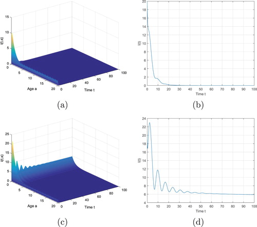
First, we fix $\psi =0.006$. If we take ${\beta }^{\ast }=1.527$, then the basic reproduction number ${\mathcal{R}}_0=\left(\mathrm{\Lambda }/(\mu +p(1-K\left)\right)\right)K_1\approx 0.9927<1$. It follows from Theorem 5.1 that the disease-free equilibrium $E_0$ is globally asymptotically stable. (a) and (b) of Figure 1 show this fact. Then we enlarge the transmission rate to ${\beta }^{\ast }=6.667$ and have ${\mathcal{R}}_0\approx 4.3361>1$. (c) and (d) of Figure 1 indicates that the endemic equilibrium $E^{\ast }$ is asymptotically stable, which supports Theorem 5.3.

Figure 1. Time evolution of the infective population $i(t,a)$, $0\le t\le 100$, $0\le a\le 20$ for system (2(2) $\begin{array}{rl}& \frac{\mathrm{d}S\left(t\right)}{\mathrm{d}t}=\mathrm{\Lambda }-\mu S\left(t\right)-f\left(S\right(t),J(t\left)\right)-\phi S\left(t\right)+{\int }_0^{\mathrm{\infty }}\epsilon \left(a\right)v(t,a)\mathrm{d}a,\\ & \frac{\mathrm{\partial }i(t,a)}{\mathrm{\partial }t}+\frac{\mathrm{\partial }i(t,a)}{\mathrm{\partial }a}=-(\mu +\gamma (a)+\delta (a\left)\right)i(t,a),\\ & i(t,0)=f\left(S\right(t),J(t\left)\right),J\left(t\right)={\int }_0^{\mathrm{\infty }}\beta \left(a\right)i(t,a)\mathrm{d}a,\\ & \frac{\mathrm{\partial }v(t,a)}{\mathrm{\partial }t}+\frac{\mathrm{\partial }v(t,a)}{\mathrm{\partial }a}=-(\mu +\epsilon (a\left)\right)v(t,a),\\ & v(t,0)=\phi S\left(t\right),\end{array}$(2) ) with initial value $i_0\left(a\right)=1+\cos (-2a)$ and $v_0\left(a\right)={\mathrm{e}}^{-a}$. (a) and (b) with ${\beta }^{\ast }=1.527$, (c) and (d) with ${\beta }^{\ast }=6.667$.

Next we study the effect of some parameters on the disease spread.

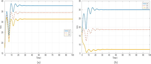
Vaccination plays an important role in controlling the disease prevalence. (a) of Figure 2 indicates that improving the vaccine coverage for the susceptible decreases the final size of the disease prevalence. In fact, improving the vaccine rate can reduce the basic reproduction number. Theorem 5.1 implies that taking suitable vaccine measures can slow down the disease prevalence and even make the disease die out. (b) of Figure 2 shows that taking vaccine on newborns has the familiar effect as increasing φ.

Figure 2. Time evolution of the infective population $i(t,a)$, $0\le t\le 100$, $0\le a\le 20$ for system (2(2) $\begin{array}{rl}& \frac{\mathrm{d}S\left(t\right)}{\mathrm{d}t}=\mathrm{\Lambda }-\mu S\left(t\right)-f\left(S\right(t),J(t\left)\right)-\phi S\left(t\right)+{\int }_0^{\mathrm{\infty }}\epsilon \left(a\right)v(t,a)\mathrm{d}a,\\ & \frac{\mathrm{\partial }i(t,a)}{\mathrm{\partial }t}+\frac{\mathrm{\partial }i(t,a)}{\mathrm{\partial }a}=-(\mu +\gamma (a)+\delta (a\left)\right)i(t,a),\\ & i(t,0)=f\left(S\right(t),J(t\left)\right),J\left(t\right)={\int }_0^{\mathrm{\infty }}\beta \left(a\right)i(t,a)\mathrm{d}a,\\ & \frac{\mathrm{\partial }v(t,a)}{\mathrm{\partial }t}+\frac{\mathrm{\partial }v(t,a)}{\mathrm{\partial }a}=-(\mu +\epsilon (a\left)\right)v(t,a),\\ & v(t,0)=\phi S\left(t\right),\end{array}$(2) ) with different vaccinated rates and input rate. (a) with $\phi =0.3,0.4,\mathrm{0.5.}$ (b) with $\mathrm{\Lambda }=10,20,40$.

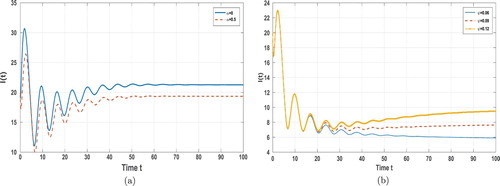
As for the transmission rate, we take α to be 0 and 0.5, respectively. Whenever we take any value for α, the value of the basic reproduction number doesn't change any more. Since ${\mathcal{R}}_0>1$, Theorem 5.3 implies that the disease must break out. From (a) of Figure 3, we see that enlarging α can lower the final size of the disease (the value of the component I of the endemic equilibrium). Furthermore, we readily see that enlarging the immunity waning rate can raise the value of the basic reproduction number. Hence this move increases the transmission risk. (b) of Figure 3 shows that the final size of the disease increases as the immunity waning rate increases.

Figure 3. Time evolution of the infective population $i(t,a)$, $0\le t\le 100$, $0\le a\le 20$ for system (2(2) $\begin{array}{rl}& \frac{\mathrm{d}S\left(t\right)}{\mathrm{d}t}=\mathrm{\Lambda }-\mu S\left(t\right)-f\left(S\right(t),J(t\left)\right)-\phi S\left(t\right)+{\int }_0^{\mathrm{\infty }}\epsilon \left(a\right)v(t,a)\mathrm{d}a,\\ & \frac{\mathrm{\partial }i(t,a)}{\mathrm{\partial }t}+\frac{\mathrm{\partial }i(t,a)}{\mathrm{\partial }a}=-(\mu +\gamma (a)+\delta (a\left)\right)i(t,a),\\ & i(t,0)=f\left(S\right(t),J(t\left)\right),J\left(t\right)={\int }_0^{\mathrm{\infty }}\beta \left(a\right)i(t,a)\mathrm{d}a,\\ & \frac{\mathrm{\partial }v(t,a)}{\mathrm{\partial }t}+\frac{\mathrm{\partial }v(t,a)}{\mathrm{\partial }a}=-(\mu +\epsilon (a\left)\right)v(t,a),\\ & v(t,0)=\phi S\left(t\right),\end{array}$(2) ) with different transmission rates and different immunity waning rates. (a) with different values $\alpha =0,0.5$, (b) with different immunity waning rates $\psi =0.06,0.09,0.12$.

7. Conclusion and discussion

We proposed a general SIVS model with infection age and vaccinated age. It turned out that the dynamics of the model is determined by the basic reproduction number ${\mathcal{R}}_0$, which determines whether the disease dies out or persists. Our model generalizes many existing ones with some being listed in Table 2. Here f, F, G have familiar features as Assumption of (B1) in our paper. Moreover, the idea of this paper can be applied to some other structured epidemic models such as SVIR [6], SEIR [13,19] models, and even if two-group model [21].

Table 2. Incidence rates.

Models	Incidence Rates	References
SIVS	$S\left(t\right){\int }_0^{\mathrm{\infty }}\beta \left(a\right)i(t,a)da$	[18,22,31]
SIR(PDE)	$\begin{array}{c}f(S,J)\\ S{\int }_0^{\mathrm{\infty }}\beta \left(a\right)f\left(i\right(t,a\left)\right)\mathrm{d}a\end{array}$	[24]
		[4]
SIR(ODE,DDE)	$\begin{array}{c}f(S,I)\\ F\left(S\right)G\left(I\right(t-\tau \left)\right)\end{array}$	[16]
		[3]

In this paper, we mainly focus on the global stability of equilibria. However, some complex phenomena such as multiple endemic equilibria (backward bifurcations) [18,29] and unstable endemic equilibrium [1,2,26] have appeared in some epidemic models with vaccination. In the future, we shall address them with more age structures.

Disclosure statement

There is no any potential conflict of interest in this work.

Additional information

Funding

Research is partially supported by the National Natural Science Foundation of China [Nos. 61573016,61203228,11371313], Shanxi Scholarship Council of China (2015-094), Shanxi Scientific Data Sharing Platform for Animal Diseases, and the Natural Sciences and Engineering Research Council (NSERC) of Canada.

References

- V. Andreasen, Instability in an SIR-model with age-dependent susceptibility, in Mathematical Population Dynamics: Analysis of Heterogeneity, O. Arino, M. Kimmel and M. Langlais, eds., Wuerz Publ., Winnipeg, 1995, pp. 3–14.
- Y. Cha, M. Iannelli, and F.A. Milner, Stability change of an epidemic model, Dynam. Syst. Appl. 9 (2000), pp. 361–376.
- Y. Chen, J. Yang and F. Zhang, The global stability of an SIRS model with infection age, Math. Biosci. Eng. 11 (2014), pp. 449–469. doi: 10.3934/mbe.2014.11.449
- Y. Chen, S. Zou, and J. Yang, Global analysis of an SIR epidemic model with infection age and saturated incidence, Nonlinear Anal. Real World Appl. 30 (2016), pp. 16–31. doi: 10.1016/j.nonrwa.2015.11.001
- D. Ding and X. Ding, Global stability of multi-group vaccination epidemic models with delays, Nonlinear Anal. Real World Appl. 12 (2011), pp. 1991–1997. doi: 10.1016/j.nonrwa.2010.12.015
- X. Duan, S. Yuan, and X. Li, Global stability of an SVIR model with age of vaccination, Appl. Math. Comput. 226 (2014), pp. 528–540.
- X. Duan, S. Yuan, Z. Qiu, and J. Ma, Global stability of an SVEIR epidemic model with ages of vaccination and latency, Comput. Math. Appl. 68 (2014), pp. 288–308. doi: 10.1016/j.camwa.2014.06.002
- Z. Feng and H.R. Thieme, Endemic models with arbitrarily distributed periods of infection I: Fundamental properties of the model, SIAM J. Appl. Math. 61 (2000), pp. 803–833. doi: 10.1137/S0036139998347834
- D.P. Francis, P.M. Feorino, J.R. Broderson, H.M. Mcclure, J.P. Getchell, C.R. Mcgrath, B. Swenson, J.S. Mcdougal, E.L. Palmer, A.K. Harrison, F. Barre-Sinoussi, J.-C. Chermann, L.Montagnier, J.W. Curran, C.D. Cabradilla, and V.S. Kalyanaraman, Infection of chimpanzees with lymphadenopathy-associated virus, Lancet 2 (1984), pp. 1276–1277. doi: 10.1016/S0140-6736(84)92824-1
- H. Gulbudak and M. Martcheva, A Structured avian influenza model with imperfect vaccination and vaccine induced asymptomatic infection, Bull. Math. Biol. 76(10) (2014), pp. 2389–2425. doi: 10.1007/s11538-014-0012-1
- J.K. Hale, Asymptotic Behavior of Dissipative Systems, AMS, Providence, 1988.
- W.M. Hirsch, H. Hanisch, and J.P. Gabriel, Differential equation models of some parasitic infections: Methods for the study of asymptotic behavior, Comm. Pure Appl. Math. 38 (1985), pp. 733–753. doi: 10.1002/cpa.3160380607
- G. Huang, Y. Takeuchi, W. Ma, and D. Wei, Global stability for delay SIR and SEIR epidemic models with nonlinear incidence rate, Bull. Math. Biol. 72 (2010), pp. 1192–1207. doi: 10.1007/s11538-009-9487-6
- M. Iannelli, Mathematical Theory of Age-Structured Population Dynamics, Applied Mathematics Monographs, vol. 7, Giardini Editorie Stampatori, Pisa, 1995.
- M. Iannelli, M. Martcheva, and X.-Z. Li, Strain replacement in an epidemic model with super-infection and perfect vaccination, Math. Biosci. 195 (2005), pp. 23–46. doi: 10.1016/j.mbs.2005.01.004
- A. Korobeinikov, Lyapunov functions and global stability for SIR and SIRS epidemiological models with non-linear transmission, Bull. Math. Biol. 68 (2006), pp. 615–626. doi: 10.1007/s11538-005-9037-9
- A. Korobeinikov and P.K. Maini, Nonlinear incidence and stability of infectious disease models, Math. Med. Biol. 22 (2005), pp. 113–128. doi: 10.1093/imammb/dqi001
- X. Li, J. Wang, and M. Ghosh, Stability and bifurcation of an SIVS epidemic model with treatment and age of vaccination, Appl. Math. Model. 34 (2010), pp. 437–450. doi: 10.1016/j.apm.2009.06.002
- J. Li, Y. Yang, and Y. Zhou, Global stability of an epidemic model with latent stage and vaccination, Nonlinear Anal. Real World Appl. 12 (2011), pp. 2163–2173. doi: 10.1016/j.nonrwa.2010.12.030
- P. Magal, Compact attractors for time periodic age-structured population models, Electron. J. Differential Equations 65 (2001), pp. 1–35.
- P. Magal and C.C. McCluskey, Two group infection age model: An application to nosocomial infection, SIAM J. Appl. Math. 73(2) (2013), pp. 1058–1095. doi: 10.1137/120882056
- P. Magal, C.C. McCluskey, and G.F. Webb, Lyapunov functional and global asymptotic stability for an infection-age model, Appl. Anal. 89 (2010), pp. 1109–1140. doi: 10.1080/00036810903208122
- C.C. McCluskey, Global stability for an SEI epidemiological model with continuous age-structure in the exposed and infectious classes, Math. Biosci. Eng. 9 (2012), pp. 819–841. doi: 10.3934/mbe.2012.9.819
- H.L. Smith and H.R. Thieme, Dynamical Systems and Population Persistence, Grad. Stud. Math., vol. 118, AMS, Providence, RI, 2011.
- B. Soufiane and T.M. Touaoula, Global analysis of an infection age model with a class of nonlinear incidence rate, J. Math. Anal. Appl. 434 (2016), pp. 1211–1239. doi: 10.1016/j.jmaa.2015.09.066
- H.R. Thieme, Stability change of the endemic equilibrium in age-structured models for the spread of S-I-R type infectious diseases, in Differential Equations Models in Biology, Epidemiology and Ecology, S. Busenberg and M. Martelli, eds., Springer, Berlin, 92, 1991, 139–158.
- H.R. Thieme, Uniform persistence and permanence for non-autonomous semiflows in population biology, Math. Biosci. 166 (2000), pp. 173–201. doi: 10.1016/S0025-5564(00)00018-3
- J. Wang, R. Zhang, and T. Kuniya, Global dynamics for a class of age-infection HIV models with nonlinear infection rate, J. Math. Anal. Appl. 432 (2015), pp. 289–313. doi: 10.1016/j.jmaa.2015.06.040
- Y. Xiao and S. Tang, Dynamics of infection with nonlinear incidence in a simple vaccination model, Nonlinear Anal. Real World Appl. 11 (2010), pp. 4154–4163. doi: 10.1016/j.nonrwa.2010.05.002
- J. Xu and Y. Zhou, Global stability of a multi-group model with vaccination age, distributed delay and random perturbation, Math. Biosci. Eng. 12 (2015), pp. 1083–1106. doi: 10.3934/mbe.2015.12.1083
- J. Yang, M. Maia, and L. Wang, Global threshold dynamics of an SIVS model with waning vaccine-induced immunity and nonlinear incidence, Math. Biosci. 268 (2015), pp. 1–8. doi: 10.1016/j.mbs.2015.07.003
- J. Yang, X. Li, and F. Zhang, Global dynamics of a heroin epidemic model with age structure and nonlinear incidence, Int. J. Biomath. 9(3) (2016), p. 1650033. doi: 10.1142/S1793524516500339