A mathematical study to control Guinea worm disease: a case study on Chad

ABSTRACT

Global eradication of Guinea worm disease (GWD) is in the final stage but a mysterious epidemic of the parasite in dog population makes the elimination programme challenging. There is neither a vaccine nor an effective treatment against the disease and therefore intervention strategies rely on the current epidemiological understandings to control the spread of the disease. A novel mathematical model can predict the future outbreaks and it can quantify the dissemination rates of control interventions. Due to the lack of such novel models, a realistic mathematical model of GWD dynamics with human population, dog population, copepod population and the worm larvae is proposed and analyzed. Considering case data from Chad, we calibrate the model and perform global sensitivity analysis of the basic reproduction number with respect to the control parameters and copepod consumption rates. Furthermore, we investigate the impact of three control interventions: awareness of humans, isolation of infected dogs and copepod clearance from contaminated water sources. We also address the impact of combination interventions which leads to the conclusion that the combination of isolating the infected dogs and treating the contaminated ponds is a plausible way for eliminating the burden of GWD from Chad.

KEYWORDS:

• Guinea worm disease
• epidemic model
• copepods
• bifurcation analysis
• control

2010 MATHEMATICS SUBJECT CLASSIFICATION:

• 92D30

1. Introduction

Guinea worm disease (GWD), also known as Dracunculiasis, is one of humanity ancient scourges [24]. Individuals are infected by drinking water contaminated with copepods, which act as an intermediate host and the carrier of nematode larvae [19]. These nematodes affect the subcutaneous tissue as the adult female migrates through the human body, generally taking residence in the foot. If left untreated, the nematode will eject larvae when exposed to fresh water, which the host will do to alleviate the burning and itching caused by the worm; the lesion may also acquire a secondary infection if improperly cared for [16]. The infection is transmitted to copepods through ingestion of free-living worm larvae and thus the cycle continues (see, Figure 1). The pain from GWD can be debilitating, which is of great concern as outbreaks tend to occur at times of agricultural importance [18]. Since neither a vaccine nor an effective treatment is available for GWD, control strategies focus on the provision of clean water, isolation of infected dogs and changing people's behaviour.

Figure 1. Life cycle of GWD [10].

As the Guinea Worm Eradication Programme progresses toward its ultimate goal of global eradication, ongoing efforts now focus on the remaining endemic countries: Chad, Ethiopia, Mali and South Sudan [14,17]. In Chad, a provisional total of 14 GWD cases have been reported during January to October 2017 and 16 cases in the previous year [14]. Added to this, there has been the observation of even more frequent GWD infections in dogs in the same geographic area in Chad where most of the human cases have occurred, which counters the historical report where infections in dogs were rarely reported even when human infections were very common [5,23,31].

Mathematical modelling has the potential to analyse the mechanisms of transmission and the complexity of epidemiological characteristics of an infectious disease and indicate new approaches to prevent and control future epidemics. Unfortunately, there are a limited number of mathematical models for GWD dynamics [2,20,26]. Smith et al. [26] developed a mathematical model of GWD to evaluate the effectiveness of chlorination. They found that despite the theoretical potential of chlorination to complete the eradication of the disease, education is far more effective.

Although, the aforementioned studies have produced useful insights on the transmission and control of GWD, none of these studies incorporated dog infection along with copepods population explicitly. A goal of this study is to design and analyse a population-level model for GWD dynamics that incorporate human population, dog population, copepods and the worm larvae. Another goal of this paper is to study the impacts of various control interventions, namely; awareness campaigns, isolation of infected dogs and killing copepods in the affected areas. The rest of the paper is organized as follows: in the next section, the model is formulated. Dynamics of disease-free system is studied in Section 3. In Section 4, the dynamical behaviour of the system without dog population and control interventions is studied. The full model is analysed in Section 5. We have calibrated the model in Section 6. To observe the effects of some important model parameters on the basic reproduction number, we performed global sensitivity analysis in Section 7. In Section 8, the effects of control interventions on the infected human populations are investigated. Finally, the paper ends with a concluding section.

2. Formulation of the model

Here, we propose a mathematical model for GWD that incorporates human population, dog population, copepods and Guinea worm larvae. We divided the total human population into susceptible, exposed and infected class. It is assumed that susceptible human population, $S_h\left(t\right)$, acquire the disease through contaminated drinking water, i.e., consumption of copepods that are infected with Guinea worm larvae. In addition, we assume no direct transmission of the disease between humans and dogs. The dynamics of humans and dogs are considered to be SEIS-type. Further, we have taken into account the effect of awareness in the population and hence divided the exposed populations into two groups: one being unaware, $E_h^1$, and another being aware, $E_h^2$. Accordingly, the infected class of humans is of two kinds: unaware infective, $I_h^1$, and aware infective, $I_h^2$. Individuals in the $I_h^1$ class produce the free larvae of Guinea worm in fresh water, however, the aware infected people will not do so. The infected individuals become again susceptible after the worm leaves the body. Thus, the total human population, $N_h\left(t\right)$, at time t is $N_h\left(t\right)=S_h\left(t\right)+E_h^1\left(t\right)+E_h^2\left(t\right)+I_h^1\left(t\right)+I_h^2\left(t\right).$ Next, we divided the dog population into three groups: susceptible, $S_d\left(t\right)$, latently infected, $E_d\left(t\right)$, and infected dogs, $I_d\left(t\right).$ We assume that dogs acquire the infection indirectly through the consumption of fish or frogs contaminated with copepods that are infected with Guinea worm larvae. The infected dogs release Guinea worm larvae in the fresh water. Therefore, the total dog population, $N_d\left(t\right)$, at time t is $N_d\left(t\right)=S_d\left(t\right)+E_d\left(t\right)+I_d\left(t\right).$

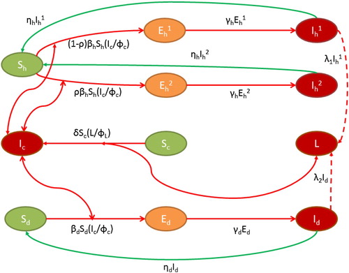
Furthermore, we assume that the copepod population is divided into susceptible copepods, $S_c\left(t\right)$, and infected copepods, $I_c\left(t\right)$. Due to short life span of copepods, we assume that once infected, they remain infected for the rest of their lives. Let $L\left(t\right)$ denote the concentration of the Guinea worm larvae in the environment. The compartmental flow diagram is depicted in Figure 2. In view of above considerations, the dynamics of GWD is governed by the following system of differential equations: (1) $\begin{array}{rl}\frac{d{S}_h}{dt}& ={\pi }_h-{\beta }_h\left(\frac{I_c}{{\phi }_c}\right)S_h-{\mu }_h{S}_h+{\eta }_h(I_h^1+I_h^2),\\ \frac{d{E}_h^1}{dt}& =(1-\rho ){\beta }_h\left(\frac{I_c}{{\phi }_c}\right)S_h-({\mu }_h+{\gamma }_h)E_h^1,\\ \frac{d{E}_h^2}{dt}& =\rho {\beta }_h\left(\frac{I_c}{{\phi }_c}\right)S_h-({\mu }_h+{\gamma }_h)E_h^2,\\ \frac{d{I}_h^1}{dt}& ={\gamma }_h{E}_h^1-({\mu }_h+{\eta }_h)I_h^1,\\ \frac{d{I}_h^2}{dt}& ={\gamma }_h{E}_h^2-({\mu }_h+{\eta }_h)I_h^2,\\ \frac{d{S}_d}{dt}& ={\pi }_d-{\beta }_d\left(\frac{I_c}{{\phi }_c}\right)S_d-{\mu }_d{S}_d+{\eta }_d{I}_d,\\ \frac{d{E}_d}{dt}& ={\beta }_d\left(\frac{I_c}{{\phi }_c}\right)S_d-({\mu }_d+{\gamma }_d)E_d,\\ \frac{d{I}_d}{dt}& ={\gamma }_d{E}_d-({\mu }_d+{\eta }_d)I_d-c{I}_d,\\ \frac{d{S}_c}{dt}& =r{N}_c\left(1-\frac{N_c}{K_c}\right)-{\beta }_h\left(\frac{S_c}{{\phi }_c}\right)N_h-{\beta }_d\left(\frac{S_c}{{\phi }_c}\right)N_d-\delta \left(\frac{L}{{\phi }_L}\right)S_c-p{S}_c,\\ \frac{d{I}_c}{dt}& =\delta \left(\frac{L}{{\phi }_L}\right)S_c-{\beta }_h\left(\frac{I_c}{{\phi }_c}\right)N_h-{\beta }_d\left(\frac{I_c}{{\phi }_c}\right)N_d-({\mu }_c+p)I_c,\\ \frac{dL}{dt}& ={\lambda }_1{I}_h^1+{\lambda }_2{I}_d-{\mu }_{L}L-\delta \left(\frac{L}{{\phi }_L}\right)N_c.\end{array}$(1)

Figure 2. Flow diagram of GWD. Two sided arrow represents new infection term, one sided arrow indicates progression to other compartments and dashed lines represent the shedding of worm larvae by infectives.

All model parameters are assumed to be positive. The biological meanings of parameters involved in the system (1(1) $\begin{array}{rl}\frac{d{S}_h}{dt}& ={\pi }_h-{\beta }_h\left(\frac{I_c}{{\phi }_c}\right)S_h-{\mu }_h{S}_h+{\eta }_h(I_h^1+I_h^2),\\ \frac{d{E}_h^1}{dt}& =(1-\rho ){\beta }_h\left(\frac{I_c}{{\phi }_c}\right)S_h-({\mu }_h+{\gamma }_h)E_h^1,\\ \frac{d{E}_h^2}{dt}& =\rho {\beta }_h\left(\frac{I_c}{{\phi }_c}\right)S_h-({\mu }_h+{\gamma }_h)E_h^2,\\ \frac{d{I}_h^1}{dt}& ={\gamma }_h{E}_h^1-({\mu }_h+{\eta }_h)I_h^1,\\ \frac{d{I}_h^2}{dt}& ={\gamma }_h{E}_h^2-({\mu }_h+{\eta }_h)I_h^2,\\ \frac{d{S}_d}{dt}& ={\pi }_d-{\beta }_d\left(\frac{I_c}{{\phi }_c}\right)S_d-{\mu }_d{S}_d+{\eta }_d{I}_d,\\ \frac{d{E}_d}{dt}& ={\beta }_d\left(\frac{I_c}{{\phi }_c}\right)S_d-({\mu }_d+{\gamma }_d)E_d,\\ \frac{d{I}_d}{dt}& ={\gamma }_d{E}_d-({\mu }_d+{\eta }_d)I_d-c{I}_d,\\ \frac{d{S}_c}{dt}& =r{N}_c\left(1-\frac{N_c}{K_c}\right)-{\beta }_h\left(\frac{S_c}{{\phi }_c}\right)N_h-{\beta }_d\left(\frac{S_c}{{\phi }_c}\right)N_d-\delta \left(\frac{L}{{\phi }_L}\right)S_c-p{S}_c,\\ \frac{d{I}_c}{dt}& =\delta \left(\frac{L}{{\phi }_L}\right)S_c-{\beta }_h\left(\frac{I_c}{{\phi }_c}\right)N_h-{\beta }_d\left(\frac{I_c}{{\phi }_c}\right)N_d-({\mu }_c+p)I_c,\\ \frac{dL}{dt}& ={\lambda }_1{I}_h^1+{\lambda }_2{I}_d-{\mu }_{L}L-\delta \left(\frac{L}{{\phi }_L}\right)N_c.\end{array}$(1) ) are given in Table 1.

Table 1. Parameter values in the model (1(1) $\begin{array}{rl}\frac{d{S}_h}{dt}& ={\pi }_h-{\beta }_h\left(\frac{I_c}{{\phi }_c}\right)S_h-{\mu }_h{S}_h+{\eta }_h(I_h^1+I_h^2),\\ \frac{d{E}_h^1}{dt}& =(1-\rho ){\beta }_h\left(\frac{I_c}{{\phi }_c}\right)S_h-({\mu }_h+{\gamma }_h)E_h^1,\\ \frac{d{E}_h^2}{dt}& =\rho {\beta }_h\left(\frac{I_c}{{\phi }_c}\right)S_h-({\mu }_h+{\gamma }_h)E_h^2,\\ \frac{d{I}_h^1}{dt}& ={\gamma }_h{E}_h^1-({\mu }_h+{\eta }_h)I_h^1,\\ \frac{d{I}_h^2}{dt}& ={\gamma }_h{E}_h^2-({\mu }_h+{\eta }_h)I_h^2,\\ \frac{d{S}_d}{dt}& ={\pi }_d-{\beta }_d\left(\frac{I_c}{{\phi }_c}\right)S_d-{\mu }_d{S}_d+{\eta }_d{I}_d,\\ \frac{d{E}_d}{dt}& ={\beta }_d\left(\frac{I_c}{{\phi }_c}\right)S_d-({\mu }_d+{\gamma }_d)E_d,\\ \frac{d{I}_d}{dt}& ={\gamma }_d{E}_d-({\mu }_d+{\eta }_d)I_d-c{I}_d,\\ \frac{d{S}_c}{dt}& =r{N}_c\left(1-\frac{N_c}{K_c}\right)-{\beta }_h\left(\frac{S_c}{{\phi }_c}\right)N_h-{\beta }_d\left(\frac{S_c}{{\phi }_c}\right)N_d-\delta \left(\frac{L}{{\phi }_L}\right)S_c-p{S}_c,\\ \frac{d{I}_c}{dt}& =\delta \left(\frac{L}{{\phi }_L}\right)S_c-{\beta }_h\left(\frac{I_c}{{\phi }_c}\right)N_h-{\beta }_d\left(\frac{I_c}{{\phi }_c}\right)N_d-({\mu }_c+p)I_c,\\ \frac{dL}{dt}& ={\lambda }_1{I}_h^1+{\lambda }_2{I}_d-{\mu }_{L}L-\delta \left(\frac{L}{{\phi }_L}\right)N_c.\end{array}$(1) ).

Parameters	Descriptions	Units	Values	Source
${\pi }_h$	Recruitment rate of humans	persons year^−1	259185	[28]
${\beta }_h$	Copepods consumption rate by humans	year^−1	1.0035e−5	Estimated
ρ	Percentage of aware human	–	Varied
${\mu }_h$	Natural death rate of humans	year^−1	0.0204	[13]
${\eta }_h$	Infectious period of humans	year^−1	0.016	Assumed
${\gamma }_h$	Incubation period of humans	year^−1	0.9996	[4]
${\pi }_d$	Recruitment rate of dogs	dogs year^−1	249983	Estimated
${\beta }_d$	Copepods consumption rate by dogs	year^−1	0.0063	Estimated
${\mu }_d$	Natural death rate of dogs	year^−1	0.0828	[30]
${\eta }_d$	Infectious period of dogs	year^−1	0.016	Assumed
${\gamma }_d$	Incubation period of dogs	year^−1	0.9996	Assumed
r	Intrinsic growth rate of copepods	year^−1	108	[3]
$K_c$	Carrying capacity of copepods	copepods	1,00,000	Assumed
${\phi }_c$	Copepod saturation constant	copepods	2,00,000	Assumed
δ	Consumption rate of larvae by copepods	year^−1	600	Assumed
${\mu }_c$	Death rate of copepods	year^−1	1.44	[7]
${\lambda }_1$	Parasite shedding rate of humans	larvae person^−1 year^−1	100	Assumed
${\lambda }_2$	Parasite shedding rate of dogs	larvae dog^−1 year^−1	100	Assumed
c	Infected dog isolation rate	year^−1	Varied
p	Clearance rate of copepods	year^−1	Varied
${\mu }_L$	Natural death rate of Guinea worm larvae	year^−1	25.92	[26]
${\phi }_L$	Guinea worm larvae saturation constant	larvae	10,000	Assumed

3. The disease-free model

In the absence of GWD, the related control parameters, i.e., ρ, p and c are assumed to be zero and therefore the system (1(1) $\begin{array}{rl}\frac{d{S}_h}{dt}& ={\pi }_h-{\beta }_h\left(\frac{I_c}{{\phi }_c}\right)S_h-{\mu }_h{S}_h+{\eta }_h(I_h^1+I_h^2),\\ \frac{d{E}_h^1}{dt}& =(1-\rho ){\beta }_h\left(\frac{I_c}{{\phi }_c}\right)S_h-({\mu }_h+{\gamma }_h)E_h^1,\\ \frac{d{E}_h^2}{dt}& =\rho {\beta }_h\left(\frac{I_c}{{\phi }_c}\right)S_h-({\mu }_h+{\gamma }_h)E_h^2,\\ \frac{d{I}_h^1}{dt}& ={\gamma }_h{E}_h^1-({\mu }_h+{\eta }_h)I_h^1,\\ \frac{d{I}_h^2}{dt}& ={\gamma }_h{E}_h^2-({\mu }_h+{\eta }_h)I_h^2,\\ \frac{d{S}_d}{dt}& ={\pi }_d-{\beta }_d\left(\frac{I_c}{{\phi }_c}\right)S_d-{\mu }_d{S}_d+{\eta }_d{I}_d,\\ \frac{d{E}_d}{dt}& ={\beta }_d\left(\frac{I_c}{{\phi }_c}\right)S_d-({\mu }_d+{\gamma }_d)E_d,\\ \frac{d{I}_d}{dt}& ={\gamma }_d{E}_d-({\mu }_d+{\eta }_d)I_d-c{I}_d,\\ \frac{d{S}_c}{dt}& =r{N}_c\left(1-\frac{N_c}{K_c}\right)-{\beta }_h\left(\frac{S_c}{{\phi }_c}\right)N_h-{\beta }_d\left(\frac{S_c}{{\phi }_c}\right)N_d-\delta \left(\frac{L}{{\phi }_L}\right)S_c-p{S}_c,\\ \frac{d{I}_c}{dt}& =\delta \left(\frac{L}{{\phi }_L}\right)S_c-{\beta }_h\left(\frac{I_c}{{\phi }_c}\right)N_h-{\beta }_d\left(\frac{I_c}{{\phi }_c}\right)N_d-({\mu }_c+p)I_c,\\ \frac{dL}{dt}& ={\lambda }_1{I}_h^1+{\lambda }_2{I}_d-{\mu }_{L}L-\delta \left(\frac{L}{{\phi }_L}\right)N_c.\end{array}$(1) ) reduces to the following subsystem: (2) $\begin{array}{rl}\frac{d{S}_h}{dt}& ={\pi }_h-{\mu }_h{S}_h,\\ \frac{d{S}_d}{dt}& ={\pi }_d-{\mu }_d{S}_d,\\ \frac{d{S}_c}{dt}& =r{S}_c\left(1-\frac{S_c}{K_c}\right)-{\beta }_h\left(\frac{S_c}{{\phi }_c}\right)S_h-{\beta }_d\left(\frac{S_c}{{\phi }_c}\right)S_d.\end{array}$(2)

3.1. Equilibrium analysis

When modelling infectious diseases, the most important issue that arises is whether the disease spread could attain endemic level or it could be eradicated. To have a better understanding of the dynamics of the disease, equilibrium and stability analysis is performed. System (2(2) $\begin{array}{rl}\frac{d{S}_h}{dt}& ={\pi }_h-{\mu }_h{S}_h,\\ \frac{d{S}_d}{dt}& ={\pi }_d-{\mu }_d{S}_d,\\ \frac{d{S}_c}{dt}& =r{S}_c\left(1-\frac{S_c}{K_c}\right)-{\beta }_h\left(\frac{S_c}{{\phi }_c}\right)S_h-{\beta }_d\left(\frac{S_c}{{\phi }_c}\right)S_d.\end{array}$(2) ) exhibits two non-negative equilibria; $E_0({\pi }_h/{\mu }_h,{\pi }_d/{\mu }_d,0)$ and $E_1({\pi }_h/{\mu }_h,{\pi }_d/{\mu }_d,{S_c}_1).$ In equilibrium $E_1$, the value of ${S_c}_1$ is given by ${S_c}_1=\left(K_c/r\right)(r-{\beta }_h{\pi }_h/{\phi }_c{\mu }_h-{\beta }_d{\pi }_d/{\phi }_c{\mu }_d).$ The equilibrium $E_0$ is always feasible and the equilibrium $E_1$ is feasible provided the following condition is satisfied: (3) $r>\frac{{\beta }_h{\pi }_h}{{\phi }_c{\mu }_h}+\frac{{\beta }_d{\pi }_d}{{\phi }_c{\mu }_d}.$(3)

3.2. Stability analysis

In this section, we perform the local stability analysis of the equilibria of the system (2(2) $\begin{array}{rl}\frac{d{S}_h}{dt}& ={\pi }_h-{\mu }_h{S}_h,\\ \frac{d{S}_d}{dt}& ={\pi }_d-{\mu }_d{S}_d,\\ \frac{d{S}_c}{dt}& =r{S}_c\left(1-\frac{S_c}{K_c}\right)-{\beta }_h\left(\frac{S_c}{{\phi }_c}\right)S_h-{\beta }_d\left(\frac{S_c}{{\phi }_c}\right)S_d.\end{array}$(2) ). This can be investigated by determining the sign of the eigenvalues of Jacobian matrix evaluated at each of the equilibrium [25]. The Jacobian of system (2(2) $\begin{array}{rl}\frac{d{S}_h}{dt}& ={\pi }_h-{\mu }_h{S}_h,\\ \frac{d{S}_d}{dt}& ={\pi }_d-{\mu }_d{S}_d,\\ \frac{d{S}_c}{dt}& =r{S}_c\left(1-\frac{S_c}{K_c}\right)-{\beta }_h\left(\frac{S_c}{{\phi }_c}\right)S_h-{\beta }_d\left(\frac{S_c}{{\phi }_c}\right)S_d.\end{array}$(2) ) is given by (4) $J=\left(\begin{array}{ccc}-{\mu }_h& 0& 0\\ 0& -{\mu }_d& 0\\ J_{31}& J_{32}& J_{33}\end{array}\right),$(4) where $J_{31}=-\frac{{\beta }_h{S}_c}{{\phi }_c},J_{32}=-\frac{{\beta }_d{S}_c}{{\phi }_c},J_{33}=r\left(1-\frac{2S_c}{K_c}\right)-\frac{{\beta }_h{S}_h}{{\phi }_c}-\frac{{\beta }_d{S}_d}{{\phi }_c}.$ Eigenvalues of the Jacobian matrix (4(4) $J=\left(\begin{array}{ccc}-{\mu }_h& 0& 0\\ 0& -{\mu }_d& 0\\ J_{31}& J_{32}& J_{33}\end{array}\right),$(4) ) evaluated at $E_0$ are real and given by ${\eta }_1=-{\mu }_h,{\eta }_2=-{\mu }_d,{\eta }_3=r-\frac{{\beta }_h{\pi }_h}{{\phi }_c{\mu }_h}-\frac{{\beta }_d{\pi }_d}{{\phi }_c{\mu }_d}.$ Under the above considerations, we establish a local stability result of the equilibrium point $E_0$ of system (2(2) $\begin{array}{rl}\frac{d{S}_h}{dt}& ={\pi }_h-{\mu }_h{S}_h,\\ \frac{d{S}_d}{dt}& ={\pi }_d-{\mu }_d{S}_d,\\ \frac{d{S}_c}{dt}& =r{S}_c\left(1-\frac{S_c}{K_c}\right)-{\beta }_h\left(\frac{S_c}{{\phi }_c}\right)S_h-{\beta }_d\left(\frac{S_c}{{\phi }_c}\right)S_d.\end{array}$(2) ), in terms of intrinsic growth rate of copepod, r.

Theorem 3.1

If $r<r_c,$ where $r_c={\beta }_h{\pi }_h/{\phi }_c{\mu }_h+{\beta }_d{\pi }_d/{\phi }_c{\mu }_d,$ then the equilibrium point $E_0$ of system (2(2) $\begin{array}{rl}\frac{d{S}_h}{dt}& ={\pi }_h-{\mu }_h{S}_h,\\ \frac{d{S}_d}{dt}& ={\pi }_d-{\mu }_d{S}_d,\\ \frac{d{S}_c}{dt}& =r{S}_c\left(1-\frac{S_c}{K_c}\right)-{\beta }_h\left(\frac{S_c}{{\phi }_c}\right)S_h-{\beta }_d\left(\frac{S_c}{{\phi }_c}\right)S_d.\end{array}$(2) ) is locally asymptotically stable and the equilibrium $E_1$ is not feasible. If $r>r_c,$ then the equilibrium point $E_1$ is feasible and the equilibrium $E_0$ becomes unstable. That is, the equilibrium $E_0$ is related to the equilibrium $E_1$ via transcritical bifurcation.

From the above theorem, it is clear that if we consider r as a bifurcation parameter, then at $r=r_c$ there is an exchange of stability properties between the equilibria $E_0$ and $E_1$. This is a clear indication of the presence of a transcritical bifurcation when $r=r_c$. The next step is to investigate the nature of the bifurcation involving $E_0$ at $r=r_c$. Observe that the eigenvalues of the matrix $J(E_0,r_c)=\left(\begin{array}{ccc}-{\mu }_h& 0& 0\\ 0& -{\mu }_d& 0\\ 0& 0& 0\end{array}\right),$ are given by ${\eta }_1=-{\mu }_h,{\eta }_2=-{\mu }_d,{\eta }_3=0.$ Since ${\eta }_3=0$ is a simple zero eigenvalue and the other eigenvalues are real and negative, therefore at $r=r_c$, the equilibrium $E_0$ is non-hyperbolic and the assumption (A1) of Theorem 4.1 in Castillo-Chavez and Song [8] is verified.

Now, denote by $\mathbf{w}=(w_1,w_2,w_3{)}^T$ a right eigenvector associated with the zero eigenvalue ${\eta }_3=0$. To determine the components of $\mathbf{w}$, we solve the following system of equations: (5) $-{\mu }_h{w}_1=0,-{\mu }_d{w}_2=0,$(5) to obtain $w_1=w_2=0$ and $w_3=1$.

Furthermore, the components of the left eigenvector $\mathbf{v}=(v_1,v_2,v_3)$ are determined by solving the following system of equations: (6) $-{\mu }_h{v}_1=0,-{\mu }_d{v}_2=0,$(6) to obtain $\mathbf{v}=(0,0,1),$ so that $\mathbf{w}.\mathbf{v}=1$.

Now, the coefficients a and b defined in Theorem 4.1 of [8] $a=\sum _{k,i,j=1}^3{v}_k{w}_i{w}_j\frac{{\mathrm{\partial }}^2{f}_k}{\mathrm{\partial }{x}_i\mathrm{\partial }{x}_j}(E_0,r_c)andb=\sum _{k,i=1}^3{v}_k{w}_i\frac{{\mathrm{\partial }}^2{f}_k}{\mathrm{\partial }{x}_i\mathrm{\partial }r}(E_0,r_c),$ may be explicitly computed. Taking into account system (2(2) $\begin{array}{rl}\frac{d{S}_h}{dt}& ={\pi }_h-{\mu }_h{S}_h,\\ \frac{d{S}_d}{dt}& ={\pi }_d-{\mu }_d{S}_d,\\ \frac{d{S}_c}{dt}& =r{S}_c\left(1-\frac{S_c}{K_c}\right)-{\beta }_h\left(\frac{S_c}{{\phi }_c}\right)S_h-{\beta }_d\left(\frac{S_c}{{\phi }_c}\right)S_d.\end{array}$(2) ), it follows that (7) $a=-\frac{2r_c}{K_c}andb=1.$(7) The previous considerations allow us to state the following theorem.

Theorem 3.2

Consider model (2(2) $\begin{array}{rl}\frac{d{S}_h}{dt}& ={\pi }_h-{\mu }_h{S}_h,\\ \frac{d{S}_d}{dt}& ={\pi }_d-{\mu }_d{S}_d,\\ \frac{d{S}_c}{dt}& =r{S}_c\left(1-\frac{S_c}{K_c}\right)-{\beta }_h\left(\frac{S_c}{{\phi }_c}\right)S_h-{\beta }_d\left(\frac{S_c}{{\phi }_c}\right)S_d.\end{array}$(2) ) and let a and b as given by (7(7) $a=-\frac{2r_c}{K_c}andb=1.$(7) ), where a<0 and b>0. The local dynamics of system (2(2) $\begin{array}{rl}\frac{d{S}_h}{dt}& ={\pi }_h-{\mu }_h{S}_h,\\ \frac{d{S}_d}{dt}& ={\pi }_d-{\mu }_d{S}_d,\\ \frac{d{S}_c}{dt}& =r{S}_c\left(1-\frac{S_c}{K_c}\right)-{\beta }_h\left(\frac{S_c}{{\phi }_c}\right)S_h-{\beta }_d\left(\frac{S_c}{{\phi }_c}\right)S_d.\end{array}$(2) ) around the equilibrium $E_0$ can be stated as

when $r<r_c$ with $r\approx r_c,$ $E_0$ is locally asymptotically stable, and there exists a negative unstable equilibrium $E_1$; when $r>r_c$ with $r\approx r_c,$ $E_0$ is unstable, and there exists a positive locally asymptotically stable equilibrium $E_1$.

Proof.

It follows from [8] Theorem 4.1 pp. 373, and Remark 1 pp. 375.

Corollary 3.3

Consider model (2(2) $\begin{array}{rl}\frac{d{S}_h}{dt}& ={\pi }_h-{\mu }_h{S}_h,\\ \frac{d{S}_d}{dt}& ={\pi }_d-{\mu }_d{S}_d,\\ \frac{d{S}_c}{dt}& =r{S}_c\left(1-\frac{S_c}{K_c}\right)-{\beta }_h\left(\frac{S_c}{{\phi }_c}\right)S_h-{\beta }_d\left(\frac{S_c}{{\phi }_c}\right)S_d.\end{array}$(2) ) and let a and b as given by (7(7) $a=-\frac{2r_c}{K_c}andb=1.$(7) ) where a<0 and b>0. At $r=r_c,$ system (2(2) $\begin{array}{rl}\frac{d{S}_h}{dt}& ={\pi }_h-{\mu }_h{S}_h,\\ \frac{d{S}_d}{dt}& ={\pi }_d-{\mu }_d{S}_d,\\ \frac{d{S}_c}{dt}& =r{S}_c\left(1-\frac{S_c}{K_c}\right)-{\beta }_h\left(\frac{S_c}{{\phi }_c}\right)S_h-{\beta }_d\left(\frac{S_c}{{\phi }_c}\right)S_d.\end{array}$(2) ) undergoes a supercritical (or forward) bifurcation.

Proof.

It is a straightforward application of Theorem 3.2.

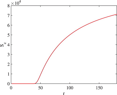
To show the occurrence of transcritical bifurcation between equilibria $E_0$ and $E_1$, we use the following set of hypothetical parameter values: ${\pi }_h=23,399$, ${\mu }_h=0.0017$, ${\pi }_d=417$, ${\mu }_d=0.0069$, $K_c=100,000$, ${\phi }_c=200,000$, ${\beta }_h=0.5$, ${\beta }_d=0.5$, and solve system (2(2) $\begin{array}{rl}\frac{d{S}_h}{dt}& ={\pi }_h-{\mu }_h{S}_h,\\ \frac{d{S}_d}{dt}& ={\pi }_d-{\mu }_d{S}_d,\\ \frac{d{S}_c}{dt}& =r{S}_c\left(1-\frac{S_c}{K_c}\right)-{\beta }_h\left(\frac{S_c}{{\phi }_c}\right)S_h-{\beta }_d\left(\frac{S_c}{{\phi }_c}\right)S_d.\end{array}$(2) ) using solver ODE15s in MATLAB 2012. The existence of transcritical bifurcation between equilibria $E_0$ and $E_1$ is shown in Figure 3. From the figure, it can be seen that there is a threshold value of r below which the equilibrium $E_0$ is stable and the equilibrium $E_1$ is not feasible and above which the equilibrium $E_0$ is unstable and the equilibrium $E_1$ is stable.

Figure 3. Transcritical bifurcation between equilibria $E_0$ and $E_1$ of system (2(2) $\begin{array}{rl}\frac{d{S}_h}{dt}& ={\pi }_h-{\mu }_h{S}_h,\\ \frac{d{S}_d}{dt}& ={\pi }_d-{\mu }_d{S}_d,\\ \frac{d{S}_c}{dt}& =r{S}_c\left(1-\frac{S_c}{K_c}\right)-{\beta }_h\left(\frac{S_c}{{\phi }_c}\right)S_h-{\beta }_d\left(\frac{S_c}{{\phi }_c}\right)S_d.\end{array}$(2) ).

Matrix J evaluated at the equilibrium $E_1$ leads to the eigenvalues $-{\mu }_h,-{\mu }_d,-\left(r-\frac{{\beta }_h{\pi }_h}{{\phi }_c{\mu }_h}-\frac{{\beta }_d{\pi }_d}{{\phi }_c{\mu }_d}\right).$ Clearly, two eigenvalues are negative and the third one is negative under the condition for the feasibility of the equilibrium $E_1$. Thus, the local stability behaviour of the equilibrium $E_1$ of the model (2(2) $\begin{array}{rl}\frac{d{S}_h}{dt}& ={\pi }_h-{\mu }_h{S}_h,\\ \frac{d{S}_d}{dt}& ={\pi }_d-{\mu }_d{S}_d,\\ \frac{d{S}_c}{dt}& =r{S}_c\left(1-\frac{S_c}{K_c}\right)-{\beta }_h\left(\frac{S_c}{{\phi }_c}\right)S_h-{\beta }_d\left(\frac{S_c}{{\phi }_c}\right)S_d.\end{array}$(2) ) can be stated in the following theorem.

Theorem 3.4

The equilibrium $E_1,$ if feasible, is locally asymptotically stable.

4. Dynamical properties of model (1) in the absence of dog population and controlinterventions

In the absence of dog populations and control interventions, system (1(1) $\begin{array}{rl}\frac{d{S}_h}{dt}& ={\pi }_h-{\beta }_h\left(\frac{I_c}{{\phi }_c}\right)S_h-{\mu }_h{S}_h+{\eta }_h(I_h^1+I_h^2),\\ \frac{d{E}_h^1}{dt}& =(1-\rho ){\beta }_h\left(\frac{I_c}{{\phi }_c}\right)S_h-({\mu }_h+{\gamma }_h)E_h^1,\\ \frac{d{E}_h^2}{dt}& =\rho {\beta }_h\left(\frac{I_c}{{\phi }_c}\right)S_h-({\mu }_h+{\gamma }_h)E_h^2,\\ \frac{d{I}_h^1}{dt}& ={\gamma }_h{E}_h^1-({\mu }_h+{\eta }_h)I_h^1,\\ \frac{d{I}_h^2}{dt}& ={\gamma }_h{E}_h^2-({\mu }_h+{\eta }_h)I_h^2,\\ \frac{d{S}_d}{dt}& ={\pi }_d-{\beta }_d\left(\frac{I_c}{{\phi }_c}\right)S_d-{\mu }_d{S}_d+{\eta }_d{I}_d,\\ \frac{d{E}_d}{dt}& ={\beta }_d\left(\frac{I_c}{{\phi }_c}\right)S_d-({\mu }_d+{\gamma }_d)E_d,\\ \frac{d{I}_d}{dt}& ={\gamma }_d{E}_d-({\mu }_d+{\eta }_d)I_d-c{I}_d,\\ \frac{d{S}_c}{dt}& =r{N}_c\left(1-\frac{N_c}{K_c}\right)-{\beta }_h\left(\frac{S_c}{{\phi }_c}\right)N_h-{\beta }_d\left(\frac{S_c}{{\phi }_c}\right)N_d-\delta \left(\frac{L}{{\phi }_L}\right)S_c-p{S}_c,\\ \frac{d{I}_c}{dt}& =\delta \left(\frac{L}{{\phi }_L}\right)S_c-{\beta }_h\left(\frac{I_c}{{\phi }_c}\right)N_h-{\beta }_d\left(\frac{I_c}{{\phi }_c}\right)N_d-({\mu }_c+p)I_c,\\ \frac{dL}{dt}& ={\lambda }_1{I}_h^1+{\lambda }_2{I}_d-{\mu }_{L}L-\delta \left(\frac{L}{{\phi }_L}\right)N_c.\end{array}$(1) ) reduces to the following subsystem: (8) $\begin{array}{rl}\frac{d{S}_h}{dt}& ={\pi }_h-{\beta }_h\left(\frac{I_c}{{\phi }_c}\right)S_h-{\mu }_h{S}_h+{\eta }_h{I}_h^1,\\ \frac{d{E}_h^1}{dt}& ={\beta }_h\left(\frac{I_c}{{\phi }_c}\right)S_h-({\mu }_h+{\gamma }_h)E_h^1,\\ \frac{d{I}_h^1}{dt}& ={\gamma }_h{E}_h^1-({\mu }_h+{\eta }_h)I_h^1,\\ \frac{d{S}_c}{dt}& =r{N}_c\left(1-\frac{N_c}{K_c}\right)-{\beta }_h\left(\frac{S_c}{{\phi }_c}\right)N_h-\delta \left(\frac{L}{{\phi }_L}\right)S_c,\\ \frac{d{I}_c}{dt}& =\delta \left(\frac{L}{{\phi }_L}\right)S_c-{\beta }_h\left(\frac{I_c}{{\phi }_c}\right)N_h-{\mu }_c{I}_c,\\ \frac{dL}{dt}& ={\lambda }_1{I}_h^1-{\mu }_{L}L-\delta \left(\frac{L}{{\phi }_L}\right)N_c.\end{array}$(8)

4.1. Positivity and boundedness of solutions

Lemma 4.1

The region of attraction for all solutions initiating in the positive octant is given by the set Ω [12,15]: (9) $\mathrm{\Omega }=\left\{\right(N_h,N_c,L):0<N_h\le Z_1,0<N_c\le Z_2,0<L\le Z_3\},$(9) where $Z_1=max\left\{\frac{{\pi }_h}{{\mu }_h},N_h\left(0\right)\right\},Z_2=max\{K_c,N_c(0\left)\right\},Z_3=max\left\{\frac{{\lambda }_1{\pi }_h}{{\mu }_h{\mu }_L},L\left(0\right)\right\}.$

4.2. Disease-free equilibria

System (8(8) $\begin{array}{rl}\frac{d{S}_h}{dt}& ={\pi }_h-{\beta }_h\left(\frac{I_c}{{\phi }_c}\right)S_h-{\mu }_h{S}_h+{\eta }_h{I}_h^1,\\ \frac{d{E}_h^1}{dt}& ={\beta }_h\left(\frac{I_c}{{\phi }_c}\right)S_h-({\mu }_h+{\gamma }_h)E_h^1,\\ \frac{d{I}_h^1}{dt}& ={\gamma }_h{E}_h^1-({\mu }_h+{\eta }_h)I_h^1,\\ \frac{d{S}_c}{dt}& =r{N}_c\left(1-\frac{N_c}{K_c}\right)-{\beta }_h\left(\frac{S_c}{{\phi }_c}\right)N_h-\delta \left(\frac{L}{{\phi }_L}\right)S_c,\\ \frac{d{I}_c}{dt}& =\delta \left(\frac{L}{{\phi }_L}\right)S_c-{\beta }_h\left(\frac{I_c}{{\phi }_c}\right)N_h-{\mu }_c{I}_c,\\ \frac{dL}{dt}& ={\lambda }_1{I}_h^1-{\mu }_{L}L-\delta \left(\frac{L}{{\phi }_L}\right)N_c.\end{array}$(8) ) exhibits two disease-free equilibria; $E_0({\pi }_h/{\mu }_h,0,0,0,0,0)$ and $E_1({\pi }_h/{\mu }_h,0,0,{S_c}_1,0,0).$ In equilibrium $E_1$, the value of ${S_c}_1$ is given by ${S_c}_1=K_c(1-1/R_c),$ where $R_c=r{\phi }_c{\mu }_h/{\beta }_h{\pi }_h.$ If $R_c>1$, then copepod population will persist otherwise, it will go extinct.

4.2.1. Basic reproduction number and stability of disease-free equilibria

The dynamics of the disease-free model (8(8) $\begin{array}{rl}\frac{d{S}_h}{dt}& ={\pi }_h-{\beta }_h\left(\frac{I_c}{{\phi }_c}\right)S_h-{\mu }_h{S}_h+{\eta }_h{I}_h^1,\\ \frac{d{E}_h^1}{dt}& ={\beta }_h\left(\frac{I_c}{{\phi }_c}\right)S_h-({\mu }_h+{\gamma }_h)E_h^1,\\ \frac{d{I}_h^1}{dt}& ={\gamma }_h{E}_h^1-({\mu }_h+{\eta }_h)I_h^1,\\ \frac{d{S}_c}{dt}& =r{N}_c\left(1-\frac{N_c}{K_c}\right)-{\beta }_h\left(\frac{S_c}{{\phi }_c}\right)N_h-\delta \left(\frac{L}{{\phi }_L}\right)S_c,\\ \frac{d{I}_c}{dt}& =\delta \left(\frac{L}{{\phi }_L}\right)S_c-{\beta }_h\left(\frac{I_c}{{\phi }_c}\right)N_h-{\mu }_c{I}_c,\\ \frac{dL}{dt}& ={\lambda }_1{I}_h^1-{\mu }_{L}L-\delta \left(\frac{L}{{\phi }_L}\right)N_c.\end{array}$(8) ) is characterized by the threshold parameter $R_{0s}$, which we refer to here as the ‘basic reproduction number, the expected number of secondary cases produced in completely susceptible population, by a typical infective individual’ for system (8(8) $\begin{array}{rl}\frac{d{S}_h}{dt}& ={\pi }_h-{\beta }_h\left(\frac{I_c}{{\phi }_c}\right)S_h-{\mu }_h{S}_h+{\eta }_h{I}_h^1,\\ \frac{d{E}_h^1}{dt}& ={\beta }_h\left(\frac{I_c}{{\phi }_c}\right)S_h-({\mu }_h+{\gamma }_h)E_h^1,\\ \frac{d{I}_h^1}{dt}& ={\gamma }_h{E}_h^1-({\mu }_h+{\eta }_h)I_h^1,\\ \frac{d{S}_c}{dt}& =r{N}_c\left(1-\frac{N_c}{K_c}\right)-{\beta }_h\left(\frac{S_c}{{\phi }_c}\right)N_h-\delta \left(\frac{L}{{\phi }_L}\right)S_c,\\ \frac{d{I}_c}{dt}& =\delta \left(\frac{L}{{\phi }_L}\right)S_c-{\beta }_h\left(\frac{I_c}{{\phi }_c}\right)N_h-{\mu }_c{I}_c,\\ \frac{dL}{dt}& ={\lambda }_1{I}_h^1-{\mu }_{L}L-\delta \left(\frac{L}{{\phi }_L}\right)N_c.\end{array}$(8) ) [9,29]. The basic reproduction number, $R_{0s}$, can be computed by seeking conditions under which a non-tirvial equilibrium exists or conditions for the existence of a transcritical bifurcation. It can also be computed using the next generation operator approach, in which case the reproduction number, $R_{0s}$, is the spectral radius of the next-generation operator $F{V}^{-1}$, where F is the matrix of new infection terms and V is the matrix of transition terms. For the system (8(8) $\begin{array}{rl}\frac{d{S}_h}{dt}& ={\pi }_h-{\beta }_h\left(\frac{I_c}{{\phi }_c}\right)S_h-{\mu }_h{S}_h+{\eta }_h{I}_h^1,\\ \frac{d{E}_h^1}{dt}& ={\beta }_h\left(\frac{I_c}{{\phi }_c}\right)S_h-({\mu }_h+{\gamma }_h)E_h^1,\\ \frac{d{I}_h^1}{dt}& ={\gamma }_h{E}_h^1-({\mu }_h+{\eta }_h)I_h^1,\\ \frac{d{S}_c}{dt}& =r{N}_c\left(1-\frac{N_c}{K_c}\right)-{\beta }_h\left(\frac{S_c}{{\phi }_c}\right)N_h-\delta \left(\frac{L}{{\phi }_L}\right)S_c,\\ \frac{d{I}_c}{dt}& =\delta \left(\frac{L}{{\phi }_L}\right)S_c-{\beta }_h\left(\frac{I_c}{{\phi }_c}\right)N_h-{\mu }_c{I}_c,\\ \frac{dL}{dt}& ={\lambda }_1{I}_h^1-{\mu }_{L}L-\delta \left(\frac{L}{{\phi }_L}\right)N_c.\end{array}$(8) ), the matrices F and V are given by $\begin{array}{rl}& F=\left(\begin{array}{cccc}0& 0& \frac{{\beta }_h{\pi }_h}{{\phi }_c{\mu }_h}& 0\\ 0& 0& 0& 0\\ 0& 0& 0& \frac{\delta {S_c}_1}{{\phi }_L}\\ 0& {\lambda }_1& 0& 0\end{array}\right),\\ & V=\left(\begin{array}{cccc}{\mu }_h+{\gamma }_h& 0& 0& 0\\ -{\gamma }_h& {\mu }_h+{\eta }_h& 0& 0\\ 0& 0& {\mu }_c+\frac{{\beta }_h{\pi }_h}{{\phi }_c{\mu }_h}& 0\\ 0& 0& 0& {\mu }_L+\frac{\delta {S_c}_1}{{\phi }_L}\end{array}\right).\end{array}$ Thus, for the system (8(8) $\begin{array}{rl}\frac{d{S}_h}{dt}& ={\pi }_h-{\beta }_h\left(\frac{I_c}{{\phi }_c}\right)S_h-{\mu }_h{S}_h+{\eta }_h{I}_h^1,\\ \frac{d{E}_h^1}{dt}& ={\beta }_h\left(\frac{I_c}{{\phi }_c}\right)S_h-({\mu }_h+{\gamma }_h)E_h^1,\\ \frac{d{I}_h^1}{dt}& ={\gamma }_h{E}_h^1-({\mu }_h+{\eta }_h)I_h^1,\\ \frac{d{S}_c}{dt}& =r{N}_c\left(1-\frac{N_c}{K_c}\right)-{\beta }_h\left(\frac{S_c}{{\phi }_c}\right)N_h-\delta \left(\frac{L}{{\phi }_L}\right)S_c,\\ \frac{d{I}_c}{dt}& =\delta \left(\frac{L}{{\phi }_L}\right)S_c-{\beta }_h\left(\frac{I_c}{{\phi }_c}\right)N_h-{\mu }_c{I}_c,\\ \frac{dL}{dt}& ={\lambda }_1{I}_h^1-{\mu }_{L}L-\delta \left(\frac{L}{{\phi }_L}\right)N_c.\end{array}$(8) ), the basic reproduction number is given by (10) $R_{0s}^3=\frac{{\beta }_h{\pi }_h\delta {\gamma }_h{\lambda }_1{K}_c\left(1-\frac{1}{R_c}\right)}{({\beta }_h{\pi }_h+{\mu }_c{\mu }_h{\phi }_c)({\eta }_h+{\mu }_h)({\gamma }_h+{\mu }_h)\left[{\mu }_L{\phi }_L+\delta K_c\left(1-\frac{1}{R_c}\right)\right]}.$(10) Regarding local stability of the disease-free equilibria $E_0$ and $E_1$ of the system (8(8) $\begin{array}{rl}\frac{d{S}_h}{dt}& ={\pi }_h-{\beta }_h\left(\frac{I_c}{{\phi }_c}\right)S_h-{\mu }_h{S}_h+{\eta }_h{I}_h^1,\\ \frac{d{E}_h^1}{dt}& ={\beta }_h\left(\frac{I_c}{{\phi }_c}\right)S_h-({\mu }_h+{\gamma }_h)E_h^1,\\ \frac{d{I}_h^1}{dt}& ={\gamma }_h{E}_h^1-({\mu }_h+{\eta }_h)I_h^1,\\ \frac{d{S}_c}{dt}& =r{N}_c\left(1-\frac{N_c}{K_c}\right)-{\beta }_h\left(\frac{S_c}{{\phi }_c}\right)N_h-\delta \left(\frac{L}{{\phi }_L}\right)S_c,\\ \frac{d{I}_c}{dt}& =\delta \left(\frac{L}{{\phi }_L}\right)S_c-{\beta }_h\left(\frac{I_c}{{\phi }_c}\right)N_h-{\mu }_c{I}_c,\\ \frac{dL}{dt}& ={\lambda }_1{I}_h^1-{\mu }_{L}L-\delta \left(\frac{L}{{\phi }_L}\right)N_c.\end{array}$(8) ), we have the following theorem.

Theorem 4.2

For system (8(8) $\begin{array}{rl}\frac{d{S}_h}{dt}& ={\pi }_h-{\beta }_h\left(\frac{I_c}{{\phi }_c}\right)S_h-{\mu }_h{S}_h+{\eta }_h{I}_h^1,\\ \frac{d{E}_h^1}{dt}& ={\beta }_h\left(\frac{I_c}{{\phi }_c}\right)S_h-({\mu }_h+{\gamma }_h)E_h^1,\\ \frac{d{I}_h^1}{dt}& ={\gamma }_h{E}_h^1-({\mu }_h+{\eta }_h)I_h^1,\\ \frac{d{S}_c}{dt}& =r{N}_c\left(1-\frac{N_c}{K_c}\right)-{\beta }_h\left(\frac{S_c}{{\phi }_c}\right)N_h-\delta \left(\frac{L}{{\phi }_L}\right)S_c,\\ \frac{d{I}_c}{dt}& =\delta \left(\frac{L}{{\phi }_L}\right)S_c-{\beta }_h\left(\frac{I_c}{{\phi }_c}\right)N_h-{\mu }_c{I}_c,\\ \frac{dL}{dt}& ={\lambda }_1{I}_h^1-{\mu }_{L}L-\delta \left(\frac{L}{{\phi }_L}\right)N_c.\end{array}$(8) ), the disease-free equilibrium $E_1$ is locally asymptotically stable if $R_{0s}<1$ and unstable if $R_{0s}>1$.

Proof.

The Jacobian of system (8(8) $\begin{array}{rl}\frac{d{S}_h}{dt}& ={\pi }_h-{\beta }_h\left(\frac{I_c}{{\phi }_c}\right)S_h-{\mu }_h{S}_h+{\eta }_h{I}_h^1,\\ \frac{d{E}_h^1}{dt}& ={\beta }_h\left(\frac{I_c}{{\phi }_c}\right)S_h-({\mu }_h+{\gamma }_h)E_h^1,\\ \frac{d{I}_h^1}{dt}& ={\gamma }_h{E}_h^1-({\mu }_h+{\eta }_h)I_h^1,\\ \frac{d{S}_c}{dt}& =r{N}_c\left(1-\frac{N_c}{K_c}\right)-{\beta }_h\left(\frac{S_c}{{\phi }_c}\right)N_h-\delta \left(\frac{L}{{\phi }_L}\right)S_c,\\ \frac{d{I}_c}{dt}& =\delta \left(\frac{L}{{\phi }_L}\right)S_c-{\beta }_h\left(\frac{I_c}{{\phi }_c}\right)N_h-{\mu }_c{I}_c,\\ \frac{dL}{dt}& ={\lambda }_1{I}_h^1-{\mu }_{L}L-\delta \left(\frac{L}{{\phi }_L}\right)N_c.\end{array}$(8) ) is given by $M=\left(\begin{array}{cccccc}{M}_{11}& 0& {\eta }_h& 0& M_{15}& 0\\ M_{21}& M_{22}& 0& 0& M_{25}& 0\\ 0& {\gamma }_h& M_{33}& 0& 0& 0\\ M_{41}& M_{42}& M_{43}& M_{44}& M_{45}& M_{46}\\ M_{51}& M_{52}& M_{53}& M_{54}& M_{55}& M_{56}\\ 0& 0& {\lambda }_1& M_{64}& M_{65}& M_{66}\end{array}\right),$ where $\begin{array}{rl}& M_{11}=-\frac{{\beta }_h{I}_c}{{\phi }_c}-{\mu }_h,M_{15}=-\frac{{\beta }_h{S}_h}{{\phi }_c},M_{21}=\frac{{\beta }_h{I}_c}{{\phi }_c},M_{22}=-({\mu }_h+{\gamma }_h),\\ & M_{25}=\frac{{\beta }_h{S}_h}{{\phi }_c},M_{33}=-({\mu }_h+{\eta }_h),M_{41}=J_{42}=J_{43}=-\frac{{\beta }_h{S}_c}{{\phi }_c},\\ & M_{44}=r\left(1-\frac{2N_c}{K_c}\right)-\frac{{\beta }_h{N}_h}{{\phi }_c}-\frac{\delta L}{{\phi }_L},M_{45}=r\left(1-\frac{2N_c}{K_c}\right),J_{46}=-\frac{\delta S_c}{{\phi }_L},\\ & M_{51}=M_{52}=M_{53}=-\frac{{\beta }_h{I}_c}{{\phi }_c},M_{54}=\frac{\delta L}{L},M_{55}=-\frac{{\beta }_h{N}_h}{{\phi }_c}-{\mu }_c,\\ & M_{56}=\frac{\delta S_c}{{\phi }_L},M_{64}=J_{65}=-\frac{\delta L}{{\phi }_L},M_{66}=-{\mu }_L-\frac{\delta N_c}{{\phi }_L}.\end{array}$ Eigenvalues of the matrix M evaluated at the equilibrium $E_0$ are $-{\mu }_h,-({\mu }_h+{\gamma }_h),-({\mu }_h+{\eta }_h),\frac{{\beta }_h{\pi }_h}{{\phi }_c{\mu }_h}(R_c-1),-\left(\frac{{\beta }_h{\pi }_h}{{\phi }_c{\mu }_h}+{\mu }_c\right),-{\mu }_L.$ Clearly, five eigenvalues are negative and one will be positive (or negative) if the equilibrium $E_1$ is feasible (not feasible). Therefore, the equilibrium $E_0$ is related to the equilibrium $E_1$ via transcritical bifurcation. Matrix M evaluated at the equilibrium $E_1$ gives two negative eigenvalues $-{\mu }_h$ and $-r{S_c}_1/K_c,$ and remaining four eigenvalues are given by $J=\left(\begin{array}{cccc}{J}_{22}-\lambda & 0& J_{25}& 0\\ {\gamma }_h& J_{33}-\lambda & 0& 0\\ 0& 0& J_{55}-\lambda & 0\\ 0& {\lambda }_1& 0& J_{66}-\lambda \end{array}\right),$ where $J_{ij}$ are values of $M_{ij}$ evaluated at the equilibrium $E_1$. The corresponding characteristic equation is given by (11) ${\lambda }^4+A_1{\lambda }^3+A_2{\lambda }^2+A_3\lambda +A_4=0,$(11) where $\begin{array}{rl}& A_1=-(J_{22}+J_{33}+J_{55}+J_{66}),\\ & A_2=J_{22}{J}_{33}+J_{55}{J}_{66}+(J_{22}+J_{33})(J_{55}+J_{66}),\\ & A_3=-J_{22}{J}_{33}(J_{55}+J_{66})-J_{55}{J}_{66}(J_{22}+J_{33}),\\ & A_4=J_{22}{J}_{33}{J}_{55}{J}_{66}-{\lambda }_1{\gamma }_h{J}_{25}{J}_{56}=J_{22}{J}_{33}{J}_{55}{J}_{66}(1-R_{0s}^3).\end{array}$ Thus, if $R_{0s}^3>1$, the equilibrium $E_1$ is unstable. Equation (11(11) ${\lambda }^4+A_1{\lambda }^3+A_2{\lambda }^2+A_3\lambda +A_4=0,$(11) ) can be written as ${\lambda }^4+A_1{\lambda }^3+A_2{\lambda }^2+A_3\lambda +J_{22}{J}_{33}{J}_{55}{J}_{66}={\lambda }_1{\gamma }_h{J}_{25}{J}_{56}.$ Since equation (12) ${\lambda }^4+A_1{\lambda }^3+A_2{\lambda }^2+A_3\lambda +J_{22}{J}_{33}{J}_{55}{J}_{66}=0$(12) has four negative roots, namely; $J_{22}$, $J_{33}$, $J_{55}$ and $J_{66}$, therefore we have $A_1>0,A_2>0,A_3>0,A_1{A}_2-A_3>0.$ Now, $\begin{array}{rl}{A}_3(A_1{A}_2-A_3)-A_1^2{A}_4& =A_3(A_1{A}_2-A_3)-A_1^2(J_{22}{J}_{33}{J}_{55}{J}_{66}-{\lambda }_1{\gamma }_h{J}_{25}{J}_{56})\\ & =A_3(A_1{A}_2-A_3)-A_2{J}_{22}{J}_{33}{J}_{55}{J}_{66}+A_1^2{\lambda }_1{\gamma }_h{J}_{25}{J}_{56}.\end{array}$ Clearly, $A_3(A_1{A}_2-A_3)-A_2{J}_{22}{J}_{33}{J}_{55}{J}_{66}$ is positive in view of signs of roots of equation (12(12) ${\lambda }^4+A_1{\lambda }^3+A_2{\lambda }^2+A_3\lambda +J_{22}{J}_{33}{J}_{55}{J}_{66}=0$(12) ). Hence, if $R_{0s}^3<1$, the equilibrium $E_1$ is locally asymptotically stable.

4.3. Existence of endemic equilibrium

From the second equilibrium equation of (8(8) $\begin{array}{rl}\frac{d{S}_h}{dt}& ={\pi }_h-{\beta }_h\left(\frac{I_c}{{\phi }_c}\right)S_h-{\mu }_h{S}_h+{\eta }_h{I}_h^1,\\ \frac{d{E}_h^1}{dt}& ={\beta }_h\left(\frac{I_c}{{\phi }_c}\right)S_h-({\mu }_h+{\gamma }_h)E_h^1,\\ \frac{d{I}_h^1}{dt}& ={\gamma }_h{E}_h^1-({\mu }_h+{\eta }_h)I_h^1,\\ \frac{d{S}_c}{dt}& =r{N}_c\left(1-\frac{N_c}{K_c}\right)-{\beta }_h\left(\frac{S_c}{{\phi }_c}\right)N_h-\delta \left(\frac{L}{{\phi }_L}\right)S_c,\\ \frac{d{I}_c}{dt}& =\delta \left(\frac{L}{{\phi }_L}\right)S_c-{\beta }_h\left(\frac{I_c}{{\phi }_c}\right)N_h-{\mu }_c{I}_c,\\ \frac{dL}{dt}& ={\lambda }_1{I}_h^1-{\mu }_{L}L-\delta \left(\frac{L}{{\phi }_L}\right)N_c.\end{array}$(8) ), we have (13) $E_h^1=\frac{{\beta }_h{S}_h{I}_c}{{\phi }_c({\mu }_h+{\gamma }_h)}.$(13) Using equation (13(13) $E_h^1=\frac{{\beta }_h{S}_h{I}_c}{{\phi }_c({\mu }_h+{\gamma }_h)}.$(13) ) in the third equilibrium equation of (8(8) $\begin{array}{rl}\frac{d{S}_h}{dt}& ={\pi }_h-{\beta }_h\left(\frac{I_c}{{\phi }_c}\right)S_h-{\mu }_h{S}_h+{\eta }_h{I}_h^1,\\ \frac{d{E}_h^1}{dt}& ={\beta }_h\left(\frac{I_c}{{\phi }_c}\right)S_h-({\mu }_h+{\gamma }_h)E_h^1,\\ \frac{d{I}_h^1}{dt}& ={\gamma }_h{E}_h^1-({\mu }_h+{\eta }_h)I_h^1,\\ \frac{d{S}_c}{dt}& =r{N}_c\left(1-\frac{N_c}{K_c}\right)-{\beta }_h\left(\frac{S_c}{{\phi }_c}\right)N_h-\delta \left(\frac{L}{{\phi }_L}\right)S_c,\\ \frac{d{I}_c}{dt}& =\delta \left(\frac{L}{{\phi }_L}\right)S_c-{\beta }_h\left(\frac{I_c}{{\phi }_c}\right)N_h-{\mu }_c{I}_c,\\ \frac{dL}{dt}& ={\lambda }_1{I}_h^1-{\mu }_{L}L-\delta \left(\frac{L}{{\phi }_L}\right)N_c.\end{array}$(8) ), we have (14) $I_h^1=\frac{{\beta }_h{\gamma }_h{S}_h{I}_c}{{\phi }_c({\mu }_h+{\eta }_h)({\mu }_h+{\gamma }_h)}.$(14) Using equation (14(14) $I_h^1=\frac{{\beta }_h{\gamma }_h{S}_h{I}_c}{{\phi }_c({\mu }_h+{\eta }_h)({\mu }_h+{\gamma }_h)}.$(14) ) in the first equilibrium equation of (8(8) $\begin{array}{rl}\frac{d{S}_h}{dt}& ={\pi }_h-{\beta }_h\left(\frac{I_c}{{\phi }_c}\right)S_h-{\mu }_h{S}_h+{\eta }_h{I}_h^1,\\ \frac{d{E}_h^1}{dt}& ={\beta }_h\left(\frac{I_c}{{\phi }_c}\right)S_h-({\mu }_h+{\gamma }_h)E_h^1,\\ \frac{d{I}_h^1}{dt}& ={\gamma }_h{E}_h^1-({\mu }_h+{\eta }_h)I_h^1,\\ \frac{d{S}_c}{dt}& =r{N}_c\left(1-\frac{N_c}{K_c}\right)-{\beta }_h\left(\frac{S_c}{{\phi }_c}\right)N_h-\delta \left(\frac{L}{{\phi }_L}\right)S_c,\\ \frac{d{I}_c}{dt}& =\delta \left(\frac{L}{{\phi }_L}\right)S_c-{\beta }_h\left(\frac{I_c}{{\phi }_c}\right)N_h-{\mu }_c{I}_c,\\ \frac{dL}{dt}& ={\lambda }_1{I}_h^1-{\mu }_{L}L-\delta \left(\frac{L}{{\phi }_L}\right)N_c.\end{array}$(8) ), we have (15) $S_h=\frac{{\pi }_h}{{\mu }_h+\frac{{\beta }_h}{{\phi }_c}\left(1+\frac{{\eta }_h{\gamma }_h}{({\mu }_h+{\eta }_h)({\mu }_h+{\gamma }_h)}\right)I_c}.$(15) Adding the first three equilibrium equations of (8(8) $\begin{array}{rl}\frac{d{S}_h}{dt}& ={\pi }_h-{\beta }_h\left(\frac{I_c}{{\phi }_c}\right)S_h-{\mu }_h{S}_h+{\eta }_h{I}_h^1,\\ \frac{d{E}_h^1}{dt}& ={\beta }_h\left(\frac{I_c}{{\phi }_c}\right)S_h-({\mu }_h+{\gamma }_h)E_h^1,\\ \frac{d{I}_h^1}{dt}& ={\gamma }_h{E}_h^1-({\mu }_h+{\eta }_h)I_h^1,\\ \frac{d{S}_c}{dt}& =r{N}_c\left(1-\frac{N_c}{K_c}\right)-{\beta }_h\left(\frac{S_c}{{\phi }_c}\right)N_h-\delta \left(\frac{L}{{\phi }_L}\right)S_c,\\ \frac{d{I}_c}{dt}& =\delta \left(\frac{L}{{\phi }_L}\right)S_c-{\beta }_h\left(\frac{I_c}{{\phi }_c}\right)N_h-{\mu }_c{I}_c,\\ \frac{dL}{dt}& ={\lambda }_1{I}_h^1-{\mu }_{L}L-\delta \left(\frac{L}{{\phi }_L}\right)N_c.\end{array}$(8) ), we get (16) $N_h=\frac{{\pi }_h}{{\mu }_h}.$(16) Adding the fourth and fifth equilibrium equations of (8(8) $\begin{array}{rl}\frac{d{S}_h}{dt}& ={\pi }_h-{\beta }_h\left(\frac{I_c}{{\phi }_c}\right)S_h-{\mu }_h{S}_h+{\eta }_h{I}_h^1,\\ \frac{d{E}_h^1}{dt}& ={\beta }_h\left(\frac{I_c}{{\phi }_c}\right)S_h-({\mu }_h+{\gamma }_h)E_h^1,\\ \frac{d{I}_h^1}{dt}& ={\gamma }_h{E}_h^1-({\mu }_h+{\eta }_h)I_h^1,\\ \frac{d{S}_c}{dt}& =r{N}_c\left(1-\frac{N_c}{K_c}\right)-{\beta }_h\left(\frac{S_c}{{\phi }_c}\right)N_h-\delta \left(\frac{L}{{\phi }_L}\right)S_c,\\ \frac{d{I}_c}{dt}& =\delta \left(\frac{L}{{\phi }_L}\right)S_c-{\beta }_h\left(\frac{I_c}{{\phi }_c}\right)N_h-{\mu }_c{I}_c,\\ \frac{dL}{dt}& ={\lambda }_1{I}_h^1-{\mu }_{L}L-\delta \left(\frac{L}{{\phi }_L}\right)N_c.\end{array}$(8) ), we get (17) $r{N}_c\left(1-\frac{N_c}{K_c}\right)-{\beta }_h\left(\frac{N_c}{{\phi }_c}\right)N_h-{\mu }_c{I}_c=0.$(17) Using the value of $N_h={\pi }_h/{\mu }_h$ in Equation (17(17) $r{N}_c\left(1-\frac{N_c}{K_c}\right)-{\beta }_h\left(\frac{N_c}{{\phi }_c}\right)N_h-{\mu }_c{I}_c=0.$(17) ) and simplifying the terms, we get the following quadratic equation in $N_c$: (18) $N_c^2-{S_c}_1{N}_c+\frac{K_c{\mu }_c{I}_c}{r}=0.$(18) Clearly, Equation (18(18) $N_c^2-{S_c}_1{N}_c+\frac{K_c{\mu }_c{I}_c}{r}=0.$(18) ) has either two or no positive roots. Let the two positive roots be $f_i\left(I_c\right),i=1,2$, then it can be given by (19) $N_c=f_i\left(I_c\right)=\frac{{S_c}_1\pm \sqrt{{S_c}_1^2-\frac{4K_c{\mu }_c{I}_c}{r}}}{2}.$(19) Using Equation (14(14) $I_h^1=\frac{{\beta }_h{\gamma }_h{S}_h{I}_c}{{\phi }_c({\mu }_h+{\eta }_h)({\mu }_h+{\gamma }_h)}.$(14) ) and the value of $N_c=f_i\left(I_c\right)$ in the last equilibrium equation of (8(8) $\begin{array}{rl}\frac{d{S}_h}{dt}& ={\pi }_h-{\beta }_h\left(\frac{I_c}{{\phi }_c}\right)S_h-{\mu }_h{S}_h+{\eta }_h{I}_h^1,\\ \frac{d{E}_h^1}{dt}& ={\beta }_h\left(\frac{I_c}{{\phi }_c}\right)S_h-({\mu }_h+{\gamma }_h)E_h^1,\\ \frac{d{I}_h^1}{dt}& ={\gamma }_h{E}_h^1-({\mu }_h+{\eta }_h)I_h^1,\\ \frac{d{S}_c}{dt}& =r{N}_c\left(1-\frac{N_c}{K_c}\right)-{\beta }_h\left(\frac{S_c}{{\phi }_c}\right)N_h-\delta \left(\frac{L}{{\phi }_L}\right)S_c,\\ \frac{d{I}_c}{dt}& =\delta \left(\frac{L}{{\phi }_L}\right)S_c-{\beta }_h\left(\frac{I_c}{{\phi }_c}\right)N_h-{\mu }_c{I}_c,\\ \frac{dL}{dt}& ={\lambda }_1{I}_h^1-{\mu }_{L}L-\delta \left(\frac{L}{{\phi }_L}\right)N_c.\end{array}$(8) ), we have (20) $L=\frac{{\lambda }_1}{{\mu }_L+\frac{\delta }{{\phi }_L}{f}_i\left(I_c\right)}\frac{{\beta }_h{\gamma }_h{S}_h{I}_c}{{\phi }_c({\mu }_h+{\eta }_h)({\mu }_h+{\gamma }_h)}=g\left(I_c\right).$(20) Now, using Equation (20(20) $L=\frac{{\lambda }_1}{{\mu }_L+\frac{\delta }{{\phi }_L}{f}_i\left(I_c\right)}\frac{{\beta }_h{\gamma }_h{S}_h{I}_c}{{\phi }_c({\mu }_h+{\eta }_h)({\mu }_h+{\gamma }_h)}=g\left(I_c\right).$(20) ) and the values of $N_h={\pi }_h/{\mu }_h$ and $N_c=f_i\left(I_c\right)$ in the fifth equilibrium equation of (8(8) $\begin{array}{rl}\frac{d{S}_h}{dt}& ={\pi }_h-{\beta }_h\left(\frac{I_c}{{\phi }_c}\right)S_h-{\mu }_h{S}_h+{\eta }_h{I}_h^1,\\ \frac{d{E}_h^1}{dt}& ={\beta }_h\left(\frac{I_c}{{\phi }_c}\right)S_h-({\mu }_h+{\gamma }_h)E_h^1,\\ \frac{d{I}_h^1}{dt}& ={\gamma }_h{E}_h^1-({\mu }_h+{\eta }_h)I_h^1,\\ \frac{d{S}_c}{dt}& =r{N}_c\left(1-\frac{N_c}{K_c}\right)-{\beta }_h\left(\frac{S_c}{{\phi }_c}\right)N_h-\delta \left(\frac{L}{{\phi }_L}\right)S_c,\\ \frac{d{I}_c}{dt}& =\delta \left(\frac{L}{{\phi }_L}\right)S_c-{\beta }_h\left(\frac{I_c}{{\phi }_c}\right)N_h-{\mu }_c{I}_c,\\ \frac{dL}{dt}& ={\lambda }_1{I}_h^1-{\mu }_{L}L-\delta \left(\frac{L}{{\phi }_L}\right)N_c.\end{array}$(8) ), we get an equation in $I_c$: $F\left(I_c\right)=0$, where (21) $F\left(I_c\right)=\frac{\delta g\left(I_c\right)}{{\phi }_L{I}_c}\left(f_i\right(I_c)-I_c)-\left({\mu }_c+\frac{{\beta }_h{\pi }_h}{{\phi }_c{\mu }_h}\right).$(21) We note the following properties of equation (21(21) $F\left(I_c\right)=\frac{\delta g\left(I_c\right)}{{\phi }_L{I}_c}\left(f_i\right(I_c)-I_c)-\left({\mu }_c+\frac{{\beta }_h{\pi }_h}{{\phi }_c{\mu }_h}\right).$(21) ):

• For $I_c=0$, the Equation (21(21) $F\left(I_c\right)=\frac{\delta g\left(I_c\right)}{{\phi }_L{I}_c}\left(f_i\right(I_c)-I_c)-\left({\mu }_c+\frac{{\beta }_h{\pi }_h}{{\phi }_c{\mu }_h}\right).$(21) ) has two roots, $f_1\left(0\right)={S_c}_1$ and $f_2\left(0\right)=0$.

• For $f_1\left(0\right)={S_c}_1$, $f_1\left(I_c\right)$ is decreasing and $F\left(0\right)>0$ if $R_{0s}>1$.

• For $f_2\left(0\right)=0$, $f_2\left(I_c\right)$ is increasing and $F\left(0\right)<0$.

• Let $I_c^{\ast }$ be such that ${S_c}_1^2=4K_c{\mu }_c{I}_c^{\ast }/r,$ then $N_c={S_c}_1/2.$

  1. For $I_c=I_c^{\ast }$, if $F\left(I_c^{\ast }\right)<0$, then there exists solution with $f_2\left(I_c\right)$.

  2. For $I_c=I_c^{\ast }$, if $F\left(I_c^{\ast }\right)>0$, then there exists solution with $f_1\left(I_c\right)$.

The above facts guarantee the existence of a positive solution of the Equation (21(21) $F\left(I_c\right)=\frac{\delta g\left(I_c\right)}{{\phi }_L{I}_c}\left(f_i\right(I_c)-I_c)-\left({\mu }_c+\frac{{\beta }_h{\pi }_h}{{\phi }_c{\mu }_h}\right).$(21) ) if $R_{0s}>1$.

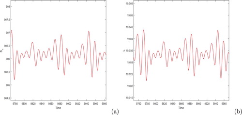
Numerically, we have seen the effect of parameter ${\lambda }_1$ on the dynamics of system (8(8) $\begin{array}{rl}\frac{d{S}_h}{dt}& ={\pi }_h-{\beta }_h\left(\frac{I_c}{{\phi }_c}\right)S_h-{\mu }_h{S}_h+{\eta }_h{I}_h^1,\\ \frac{d{E}_h^1}{dt}& ={\beta }_h\left(\frac{I_c}{{\phi }_c}\right)S_h-({\mu }_h+{\gamma }_h)E_h^1,\\ \frac{d{I}_h^1}{dt}& ={\gamma }_h{E}_h^1-({\mu }_h+{\eta }_h)I_h^1,\\ \frac{d{S}_c}{dt}& =r{N}_c\left(1-\frac{N_c}{K_c}\right)-{\beta }_h\left(\frac{S_c}{{\phi }_c}\right)N_h-\delta \left(\frac{L}{{\phi }_L}\right)S_c,\\ \frac{d{I}_c}{dt}& =\delta \left(\frac{L}{{\phi }_L}\right)S_c-{\beta }_h\left(\frac{I_c}{{\phi }_c}\right)N_h-{\mu }_c{I}_c,\\ \frac{dL}{dt}& ={\lambda }_1{I}_h^1-{\mu }_{L}L-\delta \left(\frac{L}{{\phi }_L}\right)N_c.\end{array}$(8) ). We solved the system (8(8) $\begin{array}{rl}\frac{d{S}_h}{dt}& ={\pi }_h-{\beta }_h\left(\frac{I_c}{{\phi }_c}\right)S_h-{\mu }_h{S}_h+{\eta }_h{I}_h^1,\\ \frac{d{E}_h^1}{dt}& ={\beta }_h\left(\frac{I_c}{{\phi }_c}\right)S_h-({\mu }_h+{\gamma }_h)E_h^1,\\ \frac{d{I}_h^1}{dt}& ={\gamma }_h{E}_h^1-({\mu }_h+{\eta }_h)I_h^1,\\ \frac{d{S}_c}{dt}& =r{N}_c\left(1-\frac{N_c}{K_c}\right)-{\beta }_h\left(\frac{S_c}{{\phi }_c}\right)N_h-\delta \left(\frac{L}{{\phi }_L}\right)S_c,\\ \frac{d{I}_c}{dt}& =\delta \left(\frac{L}{{\phi }_L}\right)S_c-{\beta }_h\left(\frac{I_c}{{\phi }_c}\right)N_h-{\mu }_c{I}_c,\\ \frac{dL}{dt}& ={\lambda }_1{I}_h^1-{\mu }_{L}L-\delta \left(\frac{L}{{\phi }_L}\right)N_c.\end{array}$(8) ) using solver ODE45 in MATLAB 2016a for a set of hypothetical parameter values chosen as: ${\pi }_h=0.5$, ${\beta }_h=0.65$, ${\phi }_c=5000$, ${\mu }_h=0.017$, ${\eta }_h=0.09$, ${\gamma }_h=0.01833$, r=0.27, $K_c=1000$, $\delta =0.4$, ${\phi }_L=10000$, ${\mu }_c=0.005$, ${\lambda }_1=3.5$, ${\mu }_L=0.16$, and plotted the solution trajectories in Figure 4. It is evident from the figure that the copepod and larvae populations show quasi oscillatory behaviour.

Figure 4. Time series solution of the system (8(8) $\begin{array}{rl}\frac{d{S}_h}{dt}& ={\pi }_h-{\beta }_h\left(\frac{I_c}{{\phi }_c}\right)S_h-{\mu }_h{S}_h+{\eta }_h{I}_h^1,\\ \frac{d{E}_h^1}{dt}& ={\beta }_h\left(\frac{I_c}{{\phi }_c}\right)S_h-({\mu }_h+{\gamma }_h)E_h^1,\\ \frac{d{I}_h^1}{dt}& ={\gamma }_h{E}_h^1-({\mu }_h+{\eta }_h)I_h^1,\\ \frac{d{S}_c}{dt}& =r{N}_c\left(1-\frac{N_c}{K_c}\right)-{\beta }_h\left(\frac{S_c}{{\phi }_c}\right)N_h-\delta \left(\frac{L}{{\phi }_L}\right)S_c,\\ \frac{d{I}_c}{dt}& =\delta \left(\frac{L}{{\phi }_L}\right)S_c-{\beta }_h\left(\frac{I_c}{{\phi }_c}\right)N_h-{\mu }_c{I}_c,\\ \frac{dL}{dt}& ={\lambda }_1{I}_h^1-{\mu }_{L}L-\delta \left(\frac{L}{{\phi }_L}\right)N_c.\end{array}$(8) ). Initial condition is taken as $(100,0.01,0.01,0.01,0.01,0.01)$.

Remark 4.1

In this section, we have studied the model without dog population and control interventions. As the dynamics of human and dog populations are the same, it is worthy to note that the model without human population and control interventions has the same dynamical properties as the model (8(8) $\begin{array}{rl}\frac{d{S}_h}{dt}& ={\pi }_h-{\beta }_h\left(\frac{I_c}{{\phi }_c}\right)S_h-{\mu }_h{S}_h+{\eta }_h{I}_h^1,\\ \frac{d{E}_h^1}{dt}& ={\beta }_h\left(\frac{I_c}{{\phi }_c}\right)S_h-({\mu }_h+{\gamma }_h)E_h^1,\\ \frac{d{I}_h^1}{dt}& ={\gamma }_h{E}_h^1-({\mu }_h+{\eta }_h)I_h^1,\\ \frac{d{S}_c}{dt}& =r{N}_c\left(1-\frac{N_c}{K_c}\right)-{\beta }_h\left(\frac{S_c}{{\phi }_c}\right)N_h-\delta \left(\frac{L}{{\phi }_L}\right)S_c,\\ \frac{d{I}_c}{dt}& =\delta \left(\frac{L}{{\phi }_L}\right)S_c-{\beta }_h\left(\frac{I_c}{{\phi }_c}\right)N_h-{\mu }_c{I}_c,\\ \frac{dL}{dt}& ={\lambda }_1{I}_h^1-{\mu }_{L}L-\delta \left(\frac{L}{{\phi }_L}\right)N_c.\end{array}$(8) ). Therefore, we omit the analysis of the model without human population and control interventions.

5. Dynamical properties of the full model (1)

5.1. Positivity and boundedness of solutions

Lemma 5.1

The region of attraction for all solutions of the system (1(1) $\begin{array}{rl}\frac{d{S}_h}{dt}& ={\pi }_h-{\beta }_h\left(\frac{I_c}{{\phi }_c}\right)S_h-{\mu }_h{S}_h+{\eta }_h(I_h^1+I_h^2),\\ \frac{d{E}_h^1}{dt}& =(1-\rho ){\beta }_h\left(\frac{I_c}{{\phi }_c}\right)S_h-({\mu }_h+{\gamma }_h)E_h^1,\\ \frac{d{E}_h^2}{dt}& =\rho {\beta }_h\left(\frac{I_c}{{\phi }_c}\right)S_h-({\mu }_h+{\gamma }_h)E_h^2,\\ \frac{d{I}_h^1}{dt}& ={\gamma }_h{E}_h^1-({\mu }_h+{\eta }_h)I_h^1,\\ \frac{d{I}_h^2}{dt}& ={\gamma }_h{E}_h^2-({\mu }_h+{\eta }_h)I_h^2,\\ \frac{d{S}_d}{dt}& ={\pi }_d-{\beta }_d\left(\frac{I_c}{{\phi }_c}\right)S_d-{\mu }_d{S}_d+{\eta }_d{I}_d,\\ \frac{d{E}_d}{dt}& ={\beta }_d\left(\frac{I_c}{{\phi }_c}\right)S_d-({\mu }_d+{\gamma }_d)E_d,\\ \frac{d{I}_d}{dt}& ={\gamma }_d{E}_d-({\mu }_d+{\eta }_d)I_d-c{I}_d,\\ \frac{d{S}_c}{dt}& =r{N}_c\left(1-\frac{N_c}{K_c}\right)-{\beta }_h\left(\frac{S_c}{{\phi }_c}\right)N_h-{\beta }_d\left(\frac{S_c}{{\phi }_c}\right)N_d-\delta \left(\frac{L}{{\phi }_L}\right)S_c-p{S}_c,\\ \frac{d{I}_c}{dt}& =\delta \left(\frac{L}{{\phi }_L}\right)S_c-{\beta }_h\left(\frac{I_c}{{\phi }_c}\right)N_h-{\beta }_d\left(\frac{I_c}{{\phi }_c}\right)N_d-({\mu }_c+p)I_c,\\ \frac{dL}{dt}& ={\lambda }_1{I}_h^1+{\lambda }_2{I}_d-{\mu }_{L}L-\delta \left(\frac{L}{{\phi }_L}\right)N_c.\end{array}$(1) ) initiating in the positive orthant is given by the following set [12,15]: (22) ${\mathrm{\Omega }}^{\ast }=\left\{\right(N_h,N_d,N_c,L):0<N_h\le Z_1,0<N_d\le Z_2,0<N_c\le Z_3,0<L\le Z_4\},$(22) where $\begin{array}{rl}& Z_1=max\left\{\frac{{\pi }_h}{{\mu }_h},N_h\left(0\right)\right\},Z_2=max\left\{\frac{{\pi }_d}{{\mu }_d},N_d\left(0\right)\right\},\\ & Z_3=max\{K_c,N_c(0\left)\right\},Z_4=max\left\{\frac{1}{{\mu }_L}\left(\frac{{\lambda }_1{\pi }_h}{{\mu }_h}+\frac{{\lambda }_2}{{\mu }_d}\right),L\left(0\right)\right\}.\end{array}$

Proof.

System (1(1) $\begin{array}{rl}\frac{d{S}_h}{dt}& ={\pi }_h-{\beta }_h\left(\frac{I_c}{{\phi }_c}\right)S_h-{\mu }_h{S}_h+{\eta }_h(I_h^1+I_h^2),\\ \frac{d{E}_h^1}{dt}& =(1-\rho ){\beta }_h\left(\frac{I_c}{{\phi }_c}\right)S_h-({\mu }_h+{\gamma }_h)E_h^1,\\ \frac{d{E}_h^2}{dt}& =\rho {\beta }_h\left(\frac{I_c}{{\phi }_c}\right)S_h-({\mu }_h+{\gamma }_h)E_h^2,\\ \frac{d{I}_h^1}{dt}& ={\gamma }_h{E}_h^1-({\mu }_h+{\eta }_h)I_h^1,\\ \frac{d{I}_h^2}{dt}& ={\gamma }_h{E}_h^2-({\mu }_h+{\eta }_h)I_h^2,\\ \frac{d{S}_d}{dt}& ={\pi }_d-{\beta }_d\left(\frac{I_c}{{\phi }_c}\right)S_d-{\mu }_d{S}_d+{\eta }_d{I}_d,\\ \frac{d{E}_d}{dt}& ={\beta }_d\left(\frac{I_c}{{\phi }_c}\right)S_d-({\mu }_d+{\gamma }_d)E_d,\\ \frac{d{I}_d}{dt}& ={\gamma }_d{E}_d-({\mu }_d+{\eta }_d)I_d-c{I}_d,\\ \frac{d{S}_c}{dt}& =r{N}_c\left(1-\frac{N_c}{K_c}\right)-{\beta }_h\left(\frac{S_c}{{\phi }_c}\right)N_h-{\beta }_d\left(\frac{S_c}{{\phi }_c}\right)N_d-\delta \left(\frac{L}{{\phi }_L}\right)S_c-p{S}_c,\\ \frac{d{I}_c}{dt}& =\delta \left(\frac{L}{{\phi }_L}\right)S_c-{\beta }_h\left(\frac{I_c}{{\phi }_c}\right)N_h-{\beta }_d\left(\frac{I_c}{{\phi }_c}\right)N_d-({\mu }_c+p)I_c,\\ \frac{dL}{dt}& ={\lambda }_1{I}_h^1+{\lambda }_2{I}_d-{\mu }_{L}L-\delta \left(\frac{L}{{\phi }_L}\right)N_c.\end{array}$(1) ) can be rewritten in the following form: $\frac{dX}{dt}=CX+D,$$X=[S_h,E_h^1,E_h^2,I_h^1,I_h^2,S_d,E_d,I_d,S_c,I_c,L{]}^T$ and $C=\left[\begin{array}{ccccccccccc}{d}_1& 0& 0& {\eta }_h& {\eta }_h& 0& 0& 0& 0& 0& 0\\ d_2& d_3& 0& 0& 0& 0& 0& 0& 0& 0& 0\\ d_4& 0& d_3& 0& 0& 0& 0& 0& 0& 0& 0\\ 0& {\gamma }_h& 0& d_5& 0& 0& 0& 0& 0& 0& 0\\ 0& 0& {\gamma }_h& 0& d_5& 0& 0& 0& 0& 0& 0\\ 0& 0& 0& 0& 0& d_6& 0& {\eta }_d& 0& 0& 0\\ 0& 0& 0& 0& 0& d_7& d_8& 0& 0& 0& 0\\ 0& 0& 0& 0& 0& 0& {\gamma }_d& d_9& 0& 0& 0\\ 0& 0& 0& 0& 0& 0& 0& 0& d_{10}& d_{11}& 0\\ 0& 0& 0& 0& 0& 0& 0& 0& d_{12}& d_{13}& 0\\ 0& 0& 0& {\lambda }_1& 0& 0& 0& {\lambda }_2& 0& 0& d_{14}\end{array}\right],$ where $\begin{array}{rl}& d_1=-\left({\mu }_h+{\beta }_h\frac{I_c}{{\phi }_c}\right),d_2=(1-\rho ){\beta }_h\frac{I_c}{{\phi }_c},d_3=-({\mu }_h+{\gamma }_h),d_4=\rho {\beta }_h\frac{I_c}{{\phi }_c},\\ & d_5=-({\mu }_h+{\eta }_h),d_6=-\left({\mu }_d+{\beta }_d\frac{I_c}{{\phi }_c}\right),d_7={\beta }_d\frac{I_c}{{\phi }_c},d_8=-({\mu }_d+{\gamma }_d),\\ & d_9=-({\mu }_d+{\eta }_d+c),d_{10}=r\left(1-\frac{N_c}{K_c}\right)-{\beta }_h\frac{N_h}{{\phi }_c}-{\beta }_d\frac{N_d}{{\phi }_c}-\delta \frac{L}{{\phi }_L}-p,\\ & d_{11}=r\left(1-\frac{N_c}{K_c}\right),d_{12}=\delta \frac{L}{{\phi }_L},d_{13}=-{\beta }_h\frac{N_h}{{\phi }_c}-{\beta }_d\frac{N_d}{{\phi }_c}-({\mu }_c+p),\\ & d_{14}=-\left({\mu }_L+\delta \frac{N_c}{{\phi }_L}\right).\end{array}$ The vector $D=[{\pi }_h,0,0,0,0,{\pi }_d,0,0,0,0,0{]}^T$ is positive. Note that $C\left(X\right)$ has all off-diagonal entries non-negative, i.e., $C\left(X\right)$ is a Metzler matrix for all $X\in {\mathbb{R}}_{+}^{11}$, since $D\ge 0$ system (1(1) $\begin{array}{rl}\frac{d{S}_h}{dt}& ={\pi }_h-{\beta }_h\left(\frac{I_c}{{\phi }_c}\right)S_h-{\mu }_h{S}_h+{\eta }_h(I_h^1+I_h^2),\\ \frac{d{E}_h^1}{dt}& =(1-\rho ){\beta }_h\left(\frac{I_c}{{\phi }_c}\right)S_h-({\mu }_h+{\gamma }_h)E_h^1,\\ \frac{d{E}_h^2}{dt}& =\rho {\beta }_h\left(\frac{I_c}{{\phi }_c}\right)S_h-({\mu }_h+{\gamma }_h)E_h^2,\\ \frac{d{I}_h^1}{dt}& ={\gamma }_h{E}_h^1-({\mu }_h+{\eta }_h)I_h^1,\\ \frac{d{I}_h^2}{dt}& ={\gamma }_h{E}_h^2-({\mu }_h+{\eta }_h)I_h^2,\\ \frac{d{S}_d}{dt}& ={\pi }_d-{\beta }_d\left(\frac{I_c}{{\phi }_c}\right)S_d-{\mu }_d{S}_d+{\eta }_d{I}_d,\\ \frac{d{E}_d}{dt}& ={\beta }_d\left(\frac{I_c}{{\phi }_c}\right)S_d-({\mu }_d+{\gamma }_d)E_d,\\ \frac{d{I}_d}{dt}& ={\gamma }_d{E}_d-({\mu }_d+{\eta }_d)I_d-c{I}_d,\\ \frac{d{S}_c}{dt}& =r{N}_c\left(1-\frac{N_c}{K_c}\right)-{\beta }_h\left(\frac{S_c}{{\phi }_c}\right)N_h-{\beta }_d\left(\frac{S_c}{{\phi }_c}\right)N_d-\delta \left(\frac{L}{{\phi }_L}\right)S_c-p{S}_c,\\ \frac{d{I}_c}{dt}& =\delta \left(\frac{L}{{\phi }_L}\right)S_c-{\beta }_h\left(\frac{I_c}{{\phi }_c}\right)N_h-{\beta }_d\left(\frac{I_c}{{\phi }_c}\right)N_d-({\mu }_c+p)I_c,\\ \frac{dL}{dt}& ={\lambda }_1{I}_h^1+{\lambda }_2{I}_d-{\mu }_{L}L-\delta \left(\frac{L}{{\phi }_L}\right)N_c.\end{array}$(1) ) is positively invariant in ${\mathbb{R}}_{+}^{11}$ [1]. Therefore, any trajectory of the system (1(1) $\begin{array}{rl}\frac{d{S}_h}{dt}& ={\pi }_h-{\beta }_h\left(\frac{I_c}{{\phi }_c}\right)S_h-{\mu }_h{S}_h+{\eta }_h(I_h^1+I_h^2),\\ \frac{d{E}_h^1}{dt}& =(1-\rho ){\beta }_h\left(\frac{I_c}{{\phi }_c}\right)S_h-({\mu }_h+{\gamma }_h)E_h^1,\\ \frac{d{E}_h^2}{dt}& =\rho {\beta }_h\left(\frac{I_c}{{\phi }_c}\right)S_h-({\mu }_h+{\gamma }_h)E_h^2,\\ \frac{d{I}_h^1}{dt}& ={\gamma }_h{E}_h^1-({\mu }_h+{\eta }_h)I_h^1,\\ \frac{d{I}_h^2}{dt}& ={\gamma }_h{E}_h^2-({\mu }_h+{\eta }_h)I_h^2,\\ \frac{d{S}_d}{dt}& ={\pi }_d-{\beta }_d\left(\frac{I_c}{{\phi }_c}\right)S_d-{\mu }_d{S}_d+{\eta }_d{I}_d,\\ \frac{d{E}_d}{dt}& ={\beta }_d\left(\frac{I_c}{{\phi }_c}\right)S_d-({\mu }_d+{\gamma }_d)E_d,\\ \frac{d{I}_d}{dt}& ={\gamma }_d{E}_d-({\mu }_d+{\eta }_d)I_d-c{I}_d,\\ \frac{d{S}_c}{dt}& =r{N}_c\left(1-\frac{N_c}{K_c}\right)-{\beta }_h\left(\frac{S_c}{{\phi }_c}\right)N_h-{\beta }_d\left(\frac{S_c}{{\phi }_c}\right)N_d-\delta \left(\frac{L}{{\phi }_L}\right)S_c-p{S}_c,\\ \frac{d{I}_c}{dt}& =\delta \left(\frac{L}{{\phi }_L}\right)S_c-{\beta }_h\left(\frac{I_c}{{\phi }_c}\right)N_h-{\beta }_d\left(\frac{I_c}{{\phi }_c}\right)N_d-({\mu }_c+p)I_c,\\ \frac{dL}{dt}& ={\lambda }_1{I}_h^1+{\lambda }_2{I}_d-{\mu }_{L}L-\delta \left(\frac{L}{{\phi }_L}\right)N_c.\end{array}$(1) ) starting from an initial state in ${\mathbb{R}}_{+}^{11}$ remains trapped forever in ${\mathbb{R}}_{+}^{11}$.

Adding first five equations of the system (1(1) $\begin{array}{rl}\frac{d{S}_h}{dt}& ={\pi }_h-{\beta }_h\left(\frac{I_c}{{\phi }_c}\right)S_h-{\mu }_h{S}_h+{\eta }_h(I_h^1+I_h^2),\\ \frac{d{E}_h^1}{dt}& =(1-\rho ){\beta }_h\left(\frac{I_c}{{\phi }_c}\right)S_h-({\mu }_h+{\gamma }_h)E_h^1,\\ \frac{d{E}_h^2}{dt}& =\rho {\beta }_h\left(\frac{I_c}{{\phi }_c}\right)S_h-({\mu }_h+{\gamma }_h)E_h^2,\\ \frac{d{I}_h^1}{dt}& ={\gamma }_h{E}_h^1-({\mu }_h+{\eta }_h)I_h^1,\\ \frac{d{I}_h^2}{dt}& ={\gamma }_h{E}_h^2-({\mu }_h+{\eta }_h)I_h^2,\\ \frac{d{S}_d}{dt}& ={\pi }_d-{\beta }_d\left(\frac{I_c}{{\phi }_c}\right)S_d-{\mu }_d{S}_d+{\eta }_d{I}_d,\\ \frac{d{E}_d}{dt}& ={\beta }_d\left(\frac{I_c}{{\phi }_c}\right)S_d-({\mu }_d+{\gamma }_d)E_d,\\ \frac{d{I}_d}{dt}& ={\gamma }_d{E}_d-({\mu }_d+{\eta }_d)I_d-c{I}_d,\\ \frac{d{S}_c}{dt}& =r{N}_c\left(1-\frac{N_c}{K_c}\right)-{\beta }_h\left(\frac{S_c}{{\phi }_c}\right)N_h-{\beta }_d\left(\frac{S_c}{{\phi }_c}\right)N_d-\delta \left(\frac{L}{{\phi }_L}\right)S_c-p{S}_c,\\ \frac{d{I}_c}{dt}& =\delta \left(\frac{L}{{\phi }_L}\right)S_c-{\beta }_h\left(\frac{I_c}{{\phi }_c}\right)N_h-{\beta }_d\left(\frac{I_c}{{\phi }_c}\right)N_d-({\mu }_c+p)I_c,\\ \frac{dL}{dt}& ={\lambda }_1{I}_h^1+{\lambda }_2{I}_d-{\mu }_{L}L-\delta \left(\frac{L}{{\phi }_L}\right)N_c.\end{array}$(1) ), we get $\frac{d{N}_h}{dt}={\pi }_h-{\mu }_h{N}_h.$ Hence, $0\le N_h\left(t\right)\le {\pi }_h/{\mu }_h+\left(N_h\right(0)-{\pi }_h/{\mu }_h){\mathrm{e}}^{-{\pi }_h/{\mu }_h}$. Therefore, as $t\to \mathrm{\infty }$, $0\le N_h\left(t\right)\le {\pi }_h/{\mu }_h$, and for any t>0, $0\le N_h\left(t\right)\le Z_1$, where $Z_1=max\{{\pi }_h/{\mu }_h,N_h(0\left)\right\}$.

By adding the equations in the $S_d$, $E_d$ and $I_d$ compartments of the system (1(1) $\begin{array}{rl}\frac{d{S}_h}{dt}& ={\pi }_h-{\beta }_h\left(\frac{I_c}{{\phi }_c}\right)S_h-{\mu }_h{S}_h+{\eta }_h(I_h^1+I_h^2),\\ \frac{d{E}_h^1}{dt}& =(1-\rho ){\beta }_h\left(\frac{I_c}{{\phi }_c}\right)S_h-({\mu }_h+{\gamma }_h)E_h^1,\\ \frac{d{E}_h^2}{dt}& =\rho {\beta }_h\left(\frac{I_c}{{\phi }_c}\right)S_h-({\mu }_h+{\gamma }_h)E_h^2,\\ \frac{d{I}_h^1}{dt}& ={\gamma }_h{E}_h^1-({\mu }_h+{\eta }_h)I_h^1,\\ \frac{d{I}_h^2}{dt}& ={\gamma }_h{E}_h^2-({\mu }_h+{\eta }_h)I_h^2,\\ \frac{d{S}_d}{dt}& ={\pi }_d-{\beta }_d\left(\frac{I_c}{{\phi }_c}\right)S_d-{\mu }_d{S}_d+{\eta }_d{I}_d,\\ \frac{d{E}_d}{dt}& ={\beta }_d\left(\frac{I_c}{{\phi }_c}\right)S_d-({\mu }_d+{\gamma }_d)E_d,\\ \frac{d{I}_d}{dt}& ={\gamma }_d{E}_d-({\mu }_d+{\eta }_d)I_d-c{I}_d,\\ \frac{d{S}_c}{dt}& =r{N}_c\left(1-\frac{N_c}{K_c}\right)-{\beta }_h\left(\frac{S_c}{{\phi }_c}\right)N_h-{\beta }_d\left(\frac{S_c}{{\phi }_c}\right)N_d-\delta \left(\frac{L}{{\phi }_L}\right)S_c-p{S}_c,\\ \frac{d{I}_c}{dt}& =\delta \left(\frac{L}{{\phi }_L}\right)S_c-{\beta }_h\left(\frac{I_c}{{\phi }_c}\right)N_h-{\beta }_d\left(\frac{I_c}{{\phi }_c}\right)N_d-({\mu }_c+p)I_c,\\ \frac{dL}{dt}& ={\lambda }_1{I}_h^1+{\lambda }_2{I}_d-{\mu }_{L}L-\delta \left(\frac{L}{{\phi }_L}\right)N_c.\end{array}$(1) ), we get $\frac{d{N}_d}{dt}={\pi }_d-{\mu }_d{N}_d-c{I}_d\le {\pi }_d-{\mu }_d{N}_d.$ By similar arguments, we have, for any t>0, $0\le N_d\left(t\right)\le Z_2$, where $Z_2=max\{{\pi }_d/{\mu }_d,N_d(0\left)\right\}$.

By adding the equations in the $S_c$ and $I_c$ compartments of the system (1(1) $\begin{array}{rl}\frac{d{S}_h}{dt}& ={\pi }_h-{\beta }_h\left(\frac{I_c}{{\phi }_c}\right)S_h-{\mu }_h{S}_h+{\eta }_h(I_h^1+I_h^2),\\ \frac{d{E}_h^1}{dt}& =(1-\rho ){\beta }_h\left(\frac{I_c}{{\phi }_c}\right)S_h-({\mu }_h+{\gamma }_h)E_h^1,\\ \frac{d{E}_h^2}{dt}& =\rho {\beta }_h\left(\frac{I_c}{{\phi }_c}\right)S_h-({\mu }_h+{\gamma }_h)E_h^2,\\ \frac{d{I}_h^1}{dt}& ={\gamma }_h{E}_h^1-({\mu }_h+{\eta }_h)I_h^1,\\ \frac{d{I}_h^2}{dt}& ={\gamma }_h{E}_h^2-({\mu }_h+{\eta }_h)I_h^2,\\ \frac{d{S}_d}{dt}& ={\pi }_d-{\beta }_d\left(\frac{I_c}{{\phi }_c}\right)S_d-{\mu }_d{S}_d+{\eta }_d{I}_d,\\ \frac{d{E}_d}{dt}& ={\beta }_d\left(\frac{I_c}{{\phi }_c}\right)S_d-({\mu }_d+{\gamma }_d)E_d,\\ \frac{d{I}_d}{dt}& ={\gamma }_d{E}_d-({\mu }_d+{\eta }_d)I_d-c{I}_d,\\ \frac{d{S}_c}{dt}& =r{N}_c\left(1-\frac{N_c}{K_c}\right)-{\beta }_h\left(\frac{S_c}{{\phi }_c}\right)N_h-{\beta }_d\left(\frac{S_c}{{\phi }_c}\right)N_d-\delta \left(\frac{L}{{\phi }_L}\right)S_c-p{S}_c,\\ \frac{d{I}_c}{dt}& =\delta \left(\frac{L}{{\phi }_L}\right)S_c-{\beta }_h\left(\frac{I_c}{{\phi }_c}\right)N_h-{\beta }_d\left(\frac{I_c}{{\phi }_c}\right)N_d-({\mu }_c+p)I_c,\\ \frac{dL}{dt}& ={\lambda }_1{I}_h^1+{\lambda }_2{I}_d-{\mu }_{L}L-\delta \left(\frac{L}{{\phi }_L}\right)N_c.\end{array}$(1) ), we get $\frac{d{N}_c}{dt}=r{N}_c\left(1-\frac{N_c}{K_c}\right)-{\beta }_h\left(\frac{N_c}{{\phi }_c}\right)N_h-{\beta }_d\left(\frac{N_c}{{\phi }_c}\right)N_d-p{N}_c-{\mu }_c{I}_c\le r{N}_c\left(1-\frac{N_c}{K_c}\right).$ Thus, we have, for any t>0, $0\le N_c\left(t\right)\le Z_3$, where $Z_3=max\{K_c,N_c(0\left)\right\}$.

From the last equation of system (1(1) $\begin{array}{rl}\frac{d{S}_h}{dt}& ={\pi }_h-{\beta }_h\left(\frac{I_c}{{\phi }_c}\right)S_h-{\mu }_h{S}_h+{\eta }_h(I_h^1+I_h^2),\\ \frac{d{E}_h^1}{dt}& =(1-\rho ){\beta }_h\left(\frac{I_c}{{\phi }_c}\right)S_h-({\mu }_h+{\gamma }_h)E_h^1,\\ \frac{d{E}_h^2}{dt}& =\rho {\beta }_h\left(\frac{I_c}{{\phi }_c}\right)S_h-({\mu }_h+{\gamma }_h)E_h^2,\\ \frac{d{I}_h^1}{dt}& ={\gamma }_h{E}_h^1-({\mu }_h+{\eta }_h)I_h^1,\\ \frac{d{I}_h^2}{dt}& ={\gamma }_h{E}_h^2-({\mu }_h+{\eta }_h)I_h^2,\\ \frac{d{S}_d}{dt}& ={\pi }_d-{\beta }_d\left(\frac{I_c}{{\phi }_c}\right)S_d-{\mu }_d{S}_d+{\eta }_d{I}_d,\\ \frac{d{E}_d}{dt}& ={\beta }_d\left(\frac{I_c}{{\phi }_c}\right)S_d-({\mu }_d+{\gamma }_d)E_d,\\ \frac{d{I}_d}{dt}& ={\gamma }_d{E}_d-({\mu }_d+{\eta }_d)I_d-c{I}_d,\\ \frac{d{S}_c}{dt}& =r{N}_c\left(1-\frac{N_c}{K_c}\right)-{\beta }_h\left(\frac{S_c}{{\phi }_c}\right)N_h-{\beta }_d\left(\frac{S_c}{{\phi }_c}\right)N_d-\delta \left(\frac{L}{{\phi }_L}\right)S_c-p{S}_c,\\ \frac{d{I}_c}{dt}& =\delta \left(\frac{L}{{\phi }_L}\right)S_c-{\beta }_h\left(\frac{I_c}{{\phi }_c}\right)N_h-{\beta }_d\left(\frac{I_c}{{\phi }_c}\right)N_d-({\mu }_c+p)I_c,\\ \frac{dL}{dt}& ={\lambda }_1{I}_h^1+{\lambda }_2{I}_d-{\mu }_{L}L-\delta \left(\frac{L}{{\phi }_L}\right)N_c.\end{array}$(1) ), we have $\begin{array}{rl}\frac{dL}{dt}& ={\lambda }_1{I}_h^1+{\lambda }_2{I}_d-{\mu }_{L}L-\delta \left(\frac{L}{{\phi }_L}\right)N_c\\ & \le {\lambda }_1{I}_h^1+{\lambda }_2{I}_d-{\mu }_{L}L\\ & \le \frac{{\lambda }_1{\pi }_h}{{\mu }_h}+\frac{{\lambda }_2{\pi }_d}{{\pi }_d}-{\mu }_{L}L.\end{array}$ Assume that $Z_4=max\left\{\right(1/{\mu }_L\left)\right({\lambda }_1{\pi }_h/{\mu }_h+{\lambda }_2{\pi }_d/{\pi }_d),L(0\left)\right\}$. Then $0\le L\le Z_4$.

Therefore, all mathematically and biologically feasible solutions of the system (1(1) $\begin{array}{rl}\frac{d{S}_h}{dt}& ={\pi }_h-{\beta }_h\left(\frac{I_c}{{\phi }_c}\right)S_h-{\mu }_h{S}_h+{\eta }_h(I_h^1+I_h^2),\\ \frac{d{E}_h^1}{dt}& =(1-\rho ){\beta }_h\left(\frac{I_c}{{\phi }_c}\right)S_h-({\mu }_h+{\gamma }_h)E_h^1,\\ \frac{d{E}_h^2}{dt}& =\rho {\beta }_h\left(\frac{I_c}{{\phi }_c}\right)S_h-({\mu }_h+{\gamma }_h)E_h^2,\\ \frac{d{I}_h^1}{dt}& ={\gamma }_h{E}_h^1-({\mu }_h+{\eta }_h)I_h^1,\\ \frac{d{I}_h^2}{dt}& ={\gamma }_h{E}_h^2-({\mu }_h+{\eta }_h)I_h^2,\\ \frac{d{S}_d}{dt}& ={\pi }_d-{\beta }_d\left(\frac{I_c}{{\phi }_c}\right)S_d-{\mu }_d{S}_d+{\eta }_d{I}_d,\\ \frac{d{E}_d}{dt}& ={\beta }_d\left(\frac{I_c}{{\phi }_c}\right)S_d-({\mu }_d+{\gamma }_d)E_d,\\ \frac{d{I}_d}{dt}& ={\gamma }_d{E}_d-({\mu }_d+{\eta }_d)I_d-c{I}_d,\\ \frac{d{S}_c}{dt}& =r{N}_c\left(1-\frac{N_c}{K_c}\right)-{\beta }_h\left(\frac{S_c}{{\phi }_c}\right)N_h-{\beta }_d\left(\frac{S_c}{{\phi }_c}\right)N_d-\delta \left(\frac{L}{{\phi }_L}\right)S_c-p{S}_c,\\ \frac{d{I}_c}{dt}& =\delta \left(\frac{L}{{\phi }_L}\right)S_c-{\beta }_h\left(\frac{I_c}{{\phi }_c}\right)N_h-{\beta }_d\left(\frac{I_c}{{\phi }_c}\right)N_d-({\mu }_c+p)I_c,\\ \frac{dL}{dt}& ={\lambda }_1{I}_h^1+{\lambda }_2{I}_d-{\mu }_{L}L-\delta \left(\frac{L}{{\phi }_L}\right)N_c.\end{array}$(1) ) enter the region ${\mathrm{\Omega }}^{\ast }$, i.e., the region ${\mathrm{\Omega }}^{\ast }$ is attracting. Hence, it is now sufficient to study the dynamical properties of the model (1(1) $\begin{array}{rl}\frac{d{S}_h}{dt}& ={\pi }_h-{\beta }_h\left(\frac{I_c}{{\phi }_c}\right)S_h-{\mu }_h{S}_h+{\eta }_h(I_h^1+I_h^2),\\ \frac{d{E}_h^1}{dt}& =(1-\rho ){\beta }_h\left(\frac{I_c}{{\phi }_c}\right)S_h-({\mu }_h+{\gamma }_h)E_h^1,\\ \frac{d{E}_h^2}{dt}& =\rho {\beta }_h\left(\frac{I_c}{{\phi }_c}\right)S_h-({\mu }_h+{\gamma }_h)E_h^2,\\ \frac{d{I}_h^1}{dt}& ={\gamma }_h{E}_h^1-({\mu }_h+{\eta }_h)I_h^1,\\ \frac{d{I}_h^2}{dt}& ={\gamma }_h{E}_h^2-({\mu }_h+{\eta }_h)I_h^2,\\ \frac{d{S}_d}{dt}& ={\pi }_d-{\beta }_d\left(\frac{I_c}{{\phi }_c}\right)S_d-{\mu }_d{S}_d+{\eta }_d{I}_d,\\ \frac{d{E}_d}{dt}& ={\beta }_d\left(\frac{I_c}{{\phi }_c}\right)S_d-({\mu }_d+{\gamma }_d)E_d,\\ \frac{d{I}_d}{dt}& ={\gamma }_d{E}_d-({\mu }_d+{\eta }_d)I_d-c{I}_d,\\ \frac{d{S}_c}{dt}& =r{N}_c\left(1-\frac{N_c}{K_c}\right)-{\beta }_h\left(\frac{S_c}{{\phi }_c}\right)N_h-{\beta }_d\left(\frac{S_c}{{\phi }_c}\right)N_d-\delta \left(\frac{L}{{\phi }_L}\right)S_c-p{S}_c,\\ \frac{d{I}_c}{dt}& =\delta \left(\frac{L}{{\phi }_L}\right)S_c-{\beta }_h\left(\frac{I_c}{{\phi }_c}\right)N_h-{\beta }_d\left(\frac{I_c}{{\phi }_c}\right)N_d-({\mu }_c+p)I_c,\\ \frac{dL}{dt}& ={\lambda }_1{I}_h^1+{\lambda }_2{I}_d-{\mu }_{L}L-\delta \left(\frac{L}{{\phi }_L}\right)N_c.\end{array}$(1) ) in ${\mathrm{\Omega }}^{\ast }$.

5.2. Disease-free equilibria

The model (1(1) $\begin{array}{rl}\frac{d{S}_h}{dt}& ={\pi }_h-{\beta }_h\left(\frac{I_c}{{\phi }_c}\right)S_h-{\mu }_h{S}_h+{\eta }_h(I_h^1+I_h^2),\\ \frac{d{E}_h^1}{dt}& =(1-\rho ){\beta }_h\left(\frac{I_c}{{\phi }_c}\right)S_h-({\mu }_h+{\gamma }_h)E_h^1,\\ \frac{d{E}_h^2}{dt}& =\rho {\beta }_h\left(\frac{I_c}{{\phi }_c}\right)S_h-({\mu }_h+{\gamma }_h)E_h^2,\\ \frac{d{I}_h^1}{dt}& ={\gamma }_h{E}_h^1-({\mu }_h+{\eta }_h)I_h^1,\\ \frac{d{I}_h^2}{dt}& ={\gamma }_h{E}_h^2-({\mu }_h+{\eta }_h)I_h^2,\\ \frac{d{S}_d}{dt}& ={\pi }_d-{\beta }_d\left(\frac{I_c}{{\phi }_c}\right)S_d-{\mu }_d{S}_d+{\eta }_d{I}_d,\\ \frac{d{E}_d}{dt}& ={\beta }_d\left(\frac{I_c}{{\phi }_c}\right)S_d-({\mu }_d+{\gamma }_d)E_d,\\ \frac{d{I}_d}{dt}& ={\gamma }_d{E}_d-({\mu }_d+{\eta }_d)I_d-c{I}_d,\\ \frac{d{S}_c}{dt}& =r{N}_c\left(1-\frac{N_c}{K_c}\right)-{\beta }_h\left(\frac{S_c}{{\phi }_c}\right)N_h-{\beta }_d\left(\frac{S_c}{{\phi }_c}\right)N_d-\delta \left(\frac{L}{{\phi }_L}\right)S_c-p{S}_c,\\ \frac{d{I}_c}{dt}& =\delta \left(\frac{L}{{\phi }_L}\right)S_c-{\beta }_h\left(\frac{I_c}{{\phi }_c}\right)N_h-{\beta }_d\left(\frac{I_c}{{\phi }_c}\right)N_d-({\mu }_c+p)I_c,\\ \frac{dL}{dt}& ={\lambda }_1{I}_h^1+{\lambda }_2{I}_d-{\mu }_{L}L-\delta \left(\frac{L}{{\phi }_L}\right)N_c.\end{array}$(1) ) exhibits two disease-free equilibria; $E_0({\pi }_h/{\mu }_h,0,0,0,0,{\pi }_d/{\mu }_d,0,0,0,0,0)$ and $E_1({\pi }_h/{\mu }_h,0,0,0,0,{\pi }_d/{\mu }_d,0,0,{S_c}_1,0,0)$. In equilibrium $E_1$, ${S_c}_1=\left(K_c/r\right)(r-p-{\beta }_h{\pi }_h/{\phi }_c{\mu }_h-{\beta }_d{\pi }_d/{\phi }_c{\mu }_d)$. The equilibrium $E_0$ is always feasible and the equilibrium $E_1$ is feasible provided the following condition is satisfied: (23) $r>p+\frac{{\beta }_h{\pi }_h}{{\phi }_c{\mu }_h}+\frac{{\beta }_d{\pi }_d}{{\phi }_c{\mu }_d}.$(23)

5.2.1. Basic reproduction number and stability of disease-free equilibria

We apply the next-generation operator method [29] to determine $R_0$ from system (1(1) $\begin{array}{rl}\frac{d{S}_h}{dt}& ={\pi }_h-{\beta }_h\left(\frac{I_c}{{\phi }_c}\right)S_h-{\mu }_h{S}_h+{\eta }_h(I_h^1+I_h^2),\\ \frac{d{E}_h^1}{dt}& =(1-\rho ){\beta }_h\left(\frac{I_c}{{\phi }_c}\right)S_h-({\mu }_h+{\gamma }_h)E_h^1,\\ \frac{d{E}_h^2}{dt}& =\rho {\beta }_h\left(\frac{I_c}{{\phi }_c}\right)S_h-({\mu }_h+{\gamma }_h)E_h^2,\\ \frac{d{I}_h^1}{dt}& ={\gamma }_h{E}_h^1-({\mu }_h+{\eta }_h)I_h^1,\\ \frac{d{I}_h^2}{dt}& ={\gamma }_h{E}_h^2-({\mu }_h+{\eta }_h)I_h^2,\\ \frac{d{S}_d}{dt}& ={\pi }_d-{\beta }_d\left(\frac{I_c}{{\phi }_c}\right)S_d-{\mu }_d{S}_d+{\eta }_d{I}_d,\\ \frac{d{E}_d}{dt}& ={\beta }_d\left(\frac{I_c}{{\phi }_c}\right)S_d-({\mu }_d+{\gamma }_d)E_d,\\ \frac{d{I}_d}{dt}& ={\gamma }_d{E}_d-({\mu }_d+{\eta }_d)I_d-c{I}_d,\\ \frac{d{S}_c}{dt}& =r{N}_c\left(1-\frac{N_c}{K_c}\right)-{\beta }_h\left(\frac{S_c}{{\phi }_c}\right)N_h-{\beta }_d\left(\frac{S_c}{{\phi }_c}\right)N_d-\delta \left(\frac{L}{{\phi }_L}\right)S_c-p{S}_c,\\ \frac{d{I}_c}{dt}& =\delta \left(\frac{L}{{\phi }_L}\right)S_c-{\beta }_h\left(\frac{I_c}{{\phi }_c}\right)N_h-{\beta }_d\left(\frac{I_c}{{\phi }_c}\right)N_d-({\mu }_c+p)I_c,\\ \frac{dL}{dt}& ={\lambda }_1{I}_h^1+{\lambda }_2{I}_d-{\mu }_{L}L-\delta \left(\frac{L}{{\phi }_L}\right)N_c.\end{array}$(1) ). The matrices F (of new infection terms) and V (of the transition terms) are given, respectively, as follows: $\begin{array}{rl}& F=\left(\begin{array}{cccccccc}0& 0& 0& 0& 0& 0& \frac{(1-\rho ){\beta }_h{\pi }_h}{{\phi }_c{\mu }_h}& 0\\ 0& 0& 0& 0& 0& 0& \frac{\rho {\beta }_h{\pi }_h}{{\phi }_c{\mu }_h}& 0\\ 0& 0& 0& 0& 0& 0& 0& 0\\ 0& 0& 0& 0& 0& 0& 0& 0\\ 0& 0& 0& 0& 0& 0& \frac{{\beta }_d{\pi }_d}{{\phi }_c{\mu }_d}& 0\\ 0& 0& 0& 0& 0& 0& 0& 0\\ 0& 0& 0& 0& 0& 0& 0& \frac{\delta {S_c}_1}{{\phi }_L}\\ 0& 0& 0& 0& 0& 0& 0& 0\end{array}\right),\\ & V=\left(\begin{array}{ccccc}{\mu }_h+{\gamma }_h& 0& 0& 0& 0\\ 0& {\mu }_h+{\gamma }_h& 0& 0& 0\\ -{\gamma }_h& 0& {\mu }_h+{\eta }_h& 0& 0\\ 0& -{\gamma }_h& 0& {\mu }_h+{\eta }_h& 0\\ 0& 0& 0& 0& {\mu }_d+{\gamma }_d\\ 0& 0& 0& 0& -{\gamma }_d\\ 0& 0& 0& 0& 0\\ 0& 0& -{\lambda }_1& 0& 0\end{array}\right.\\ & \left.\begin{array}{ccc}0& 0& 0\\ 0& 0& 0\\ 0& 0& 0\\ 0& 0& 0\\ 0& 0& 0\\ {\mu }_d+{\eta }_d+c& 0& 0\\ 0& {\mu }_c+p+\frac{{\beta }_h{\pi }_h}{{\phi }_c{\mu }_h}+\frac{{\beta }_d{\pi }_d}{{\phi }_c{\mu }_d}& 0\\ -{\lambda }_2& 0& {\mu }_L+\frac{\delta {S_c}_1}{{\phi }_L}\end{array}\right).\end{array}$

Following [29], $R_0=\rho \left(F{V}^{-1}\right)$, where ρ is the spectral radius of the next-generation matrix $\left(F{V}^{-1}\right)$. Thus, from the model (1(1) $\begin{array}{rl}\frac{d{S}_h}{dt}& ={\pi }_h-{\beta }_h\left(\frac{I_c}{{\phi }_c}\right)S_h-{\mu }_h{S}_h+{\eta }_h(I_h^1+I_h^2),\\ \frac{d{E}_h^1}{dt}& =(1-\rho ){\beta }_h\left(\frac{I_c}{{\phi }_c}\right)S_h-({\mu }_h+{\gamma }_h)E_h^1,\\ \frac{d{E}_h^2}{dt}& =\rho {\beta }_h\left(\frac{I_c}{{\phi }_c}\right)S_h-({\mu }_h+{\gamma }_h)E_h^2,\\ \frac{d{I}_h^1}{dt}& ={\gamma }_h{E}_h^1-({\mu }_h+{\eta }_h)I_h^1,\\ \frac{d{I}_h^2}{dt}& ={\gamma }_h{E}_h^2-({\mu }_h+{\eta }_h)I_h^2,\\ \frac{d{S}_d}{dt}& ={\pi }_d-{\beta }_d\left(\frac{I_c}{{\phi }_c}\right)S_d-{\mu }_d{S}_d+{\eta }_d{I}_d,\\ \frac{d{E}_d}{dt}& ={\beta }_d\left(\frac{I_c}{{\phi }_c}\right)S_d-({\mu }_d+{\gamma }_d)E_d,\\ \frac{d{I}_d}{dt}& ={\gamma }_d{E}_d-({\mu }_d+{\eta }_d)I_d-c{I}_d,\\ \frac{d{S}_c}{dt}& =r{N}_c\left(1-\frac{N_c}{K_c}\right)-{\beta }_h\left(\frac{S_c}{{\phi }_c}\right)N_h-{\beta }_d\left(\frac{S_c}{{\phi }_c}\right)N_d-\delta \left(\frac{L}{{\phi }_L}\right)S_c-p{S}_c,\\ \frac{d{I}_c}{dt}& =\delta \left(\frac{L}{{\phi }_L}\right)S_c-{\beta }_h\left(\frac{I_c}{{\phi }_c}\right)N_h-{\beta }_d\left(\frac{I_c}{{\phi }_c}\right)N_d-({\mu }_c+p)I_c,\\ \frac{dL}{dt}& ={\lambda }_1{I}_h^1+{\lambda }_2{I}_d-{\mu }_{L}L-\delta \left(\frac{L}{{\phi }_L}\right)N_c.\end{array}$(1) ), we have the following expression for $R_0$: (24) $\begin{array}{rl}{R}_0^2& =\frac{\delta K_c\left(r-p-\frac{{\beta }_h{\pi }_h}{{\phi }_c{\mu }_h}-\frac{{\beta }_d{\pi }_d}{{\phi }_c{\mu }_d}\right)}{r{\phi }_c{\phi }_L\left({\mu }_L+\frac{\delta {S_c}_1}{{\phi }_L}\right)\left({\mu }_c+p+\frac{{\beta }_h{\pi }_h}{{\phi }_c{\mu }_h}+\frac{{\beta }_d{\pi }_d}{{\phi }_c{\mu }_d}\right)}\end{array}$(24) (25) $\begin{array}{rl}& \times \left[\frac{{\beta }_d{\pi }_d{\gamma }_d{\lambda }_2}{{\mu }_d({\mu }_d+{\eta }_d+c)({\mu }_d+{\gamma }_d)}+\frac{{\beta }_h{\pi }_h{\gamma }_h{\lambda }_1(1-\rho )}{{\mu }_h({\mu }_h+{\eta }_h)({\mu }_h+{\gamma }_h)}\right].\end{array}$(25)

Following [29], local stability of the disease-free equilibrium $E_1$ of the system (1(1) $\begin{array}{rl}\frac{d{S}_h}{dt}& ={\pi }_h-{\beta }_h\left(\frac{I_c}{{\phi }_c}\right)S_h-{\mu }_h{S}_h+{\eta }_h(I_h^1+I_h^2),\\ \frac{d{E}_h^1}{dt}& =(1-\rho ){\beta }_h\left(\frac{I_c}{{\phi }_c}\right)S_h-({\mu }_h+{\gamma }_h)E_h^1,\\ \frac{d{E}_h^2}{dt}& =\rho {\beta }_h\left(\frac{I_c}{{\phi }_c}\right)S_h-({\mu }_h+{\gamma }_h)E_h^2,\\ \frac{d{I}_h^1}{dt}& ={\gamma }_h{E}_h^1-({\mu }_h+{\eta }_h)I_h^1,\\ \frac{d{I}_h^2}{dt}& ={\gamma }_h{E}_h^2-({\mu }_h+{\eta }_h)I_h^2,\\ \frac{d{S}_d}{dt}& ={\pi }_d-{\beta }_d\left(\frac{I_c}{{\phi }_c}\right)S_d-{\mu }_d{S}_d+{\eta }_d{I}_d,\\ \frac{d{E}_d}{dt}& ={\beta }_d\left(\frac{I_c}{{\phi }_c}\right)S_d-({\mu }_d+{\gamma }_d)E_d,\\ \frac{d{I}_d}{dt}& ={\gamma }_d{E}_d-({\mu }_d+{\eta }_d)I_d-c{I}_d,\\ \frac{d{S}_c}{dt}& =r{N}_c\left(1-\frac{N_c}{K_c}\right)-{\beta }_h\left(\frac{S_c}{{\phi }_c}\right)N_h-{\beta }_d\left(\frac{S_c}{{\phi }_c}\right)N_d-\delta \left(\frac{L}{{\phi }_L}\right)S_c-p{S}_c,\\ \frac{d{I}_c}{dt}& =\delta \left(\frac{L}{{\phi }_L}\right)S_c-{\beta }_h\left(\frac{I_c}{{\phi }_c}\right)N_h-{\beta }_d\left(\frac{I_c}{{\phi }_c}\right)N_d-({\mu }_c+p)I_c,\\ \frac{dL}{dt}& ={\lambda }_1{I}_h^1+{\lambda }_2{I}_d-{\mu }_{L}L-\delta \left(\frac{L}{{\phi }_L}\right)N_c.\end{array}$(1) ) is given by the following theorem.

Theorem 5.2

For system (1(1) $\begin{array}{rl}\frac{d{S}_h}{dt}& ={\pi }_h-{\beta }_h\left(\frac{I_c}{{\phi }_c}\right)S_h-{\mu }_h{S}_h+{\eta }_h(I_h^1+I_h^2),\\ \frac{d{E}_h^1}{dt}& =(1-\rho ){\beta }_h\left(\frac{I_c}{{\phi }_c}\right)S_h-({\mu }_h+{\gamma }_h)E_h^1,\\ \frac{d{E}_h^2}{dt}& =\rho {\beta }_h\left(\frac{I_c}{{\phi }_c}\right)S_h-({\mu }_h+{\gamma }_h)E_h^2,\\ \frac{d{I}_h^1}{dt}& ={\gamma }_h{E}_h^1-({\mu }_h+{\eta }_h)I_h^1,\\ \frac{d{I}_h^2}{dt}& ={\gamma }_h{E}_h^2-({\mu }_h+{\eta }_h)I_h^2,\\ \frac{d{S}_d}{dt}& ={\pi }_d-{\beta }_d\left(\frac{I_c}{{\phi }_c}\right)S_d-{\mu }_d{S}_d+{\eta }_d{I}_d,\\ \frac{d{E}_d}{dt}& ={\beta }_d\left(\frac{I_c}{{\phi }_c}\right)S_d-({\mu }_d+{\gamma }_d)E_d,\\ \frac{d{I}_d}{dt}& ={\gamma }_d{E}_d-({\mu }_d+{\eta }_d)I_d-c{I}_d,\\ \frac{d{S}_c}{dt}& =r{N}_c\left(1-\frac{N_c}{K_c}\right)-{\beta }_h\left(\frac{S_c}{{\phi }_c}\right)N_h-{\beta }_d\left(\frac{S_c}{{\phi }_c}\right)N_d-\delta \left(\frac{L}{{\phi }_L}\right)S_c-p{S}_c,\\ \frac{d{I}_c}{dt}& =\delta \left(\frac{L}{{\phi }_L}\right)S_c-{\beta }_h\left(\frac{I_c}{{\phi }_c}\right)N_h-{\beta }_d\left(\frac{I_c}{{\phi }_c}\right)N_d-({\mu }_c+p)I_c,\\ \frac{dL}{dt}& ={\lambda }_1{I}_h^1+{\lambda }_2{I}_d-{\mu }_{L}L-\delta \left(\frac{L}{{\phi }_L}\right)N_c.\end{array}$(1) ), the disease-free equilibrium $E_1$ is locally asymptotically stable if $R_0<1$ and unstable if $R_0>1$.

Thus, if the disease starts with small influx of infected individuals (humans, dogs, copepods or Guinea worm larvae), then it will eventually die out from the population if $R_0<1$.

5.3. Existence of endemic equilibrium

From the fourth and fifth equilibrium equations of the system (1(1) $\begin{array}{rl}\frac{d{S}_h}{dt}& ={\pi }_h-{\beta }_h\left(\frac{I_c}{{\phi }_c}\right)S_h-{\mu }_h{S}_h+{\eta }_h(I_h^1+I_h^2),\\ \frac{d{E}_h^1}{dt}& =(1-\rho ){\beta }_h\left(\frac{I_c}{{\phi }_c}\right)S_h-({\mu }_h+{\gamma }_h)E_h^1,\\ \frac{d{E}_h^2}{dt}& =\rho {\beta }_h\left(\frac{I_c}{{\phi }_c}\right)S_h-({\mu }_h+{\gamma }_h)E_h^2,\\ \frac{d{I}_h^1}{dt}& ={\gamma }_h{E}_h^1-({\mu }_h+{\eta }_h)I_h^1,\\ \frac{d{I}_h^2}{dt}& ={\gamma }_h{E}_h^2-({\mu }_h+{\eta }_h)I_h^2,\\ \frac{d{S}_d}{dt}& ={\pi }_d-{\beta }_d\left(\frac{I_c}{{\phi }_c}\right)S_d-{\mu }_d{S}_d+{\eta }_d{I}_d,\\ \frac{d{E}_d}{dt}& ={\beta }_d\left(\frac{I_c}{{\phi }_c}\right)S_d-({\mu }_d+{\gamma }_d)E_d,\\ \frac{d{I}_d}{dt}& ={\gamma }_d{E}_d-({\mu }_d+{\eta }_d)I_d-c{I}_d,\\ \frac{d{S}_c}{dt}& =r{N}_c\left(1-\frac{N_c}{K_c}\right)-{\beta }_h\left(\frac{S_c}{{\phi }_c}\right)N_h-{\beta }_d\left(\frac{S_c}{{\phi }_c}\right)N_d-\delta \left(\frac{L}{{\phi }_L}\right)S_c-p{S}_c,\\ \frac{d{I}_c}{dt}& =\delta \left(\frac{L}{{\phi }_L}\right)S_c-{\beta }_h\left(\frac{I_c}{{\phi }_c}\right)N_h-{\beta }_d\left(\frac{I_c}{{\phi }_c}\right)N_d-({\mu }_c+p)I_c,\\ \frac{dL}{dt}& ={\lambda }_1{I}_h^1+{\lambda }_2{I}_d-{\mu }_{L}L-\delta \left(\frac{L}{{\phi }_L}\right)N_c.\end{array}$(1) ), we get the values of $E_h^1$ and $E_h^2$ as follows: (26) $E_h^1=\frac{({\mu }_h+{\eta }_h)I_h^1}{{\gamma }_h}={\sigma }_h{I}_h^1,E_h^2=\frac{({\mu }_h+{\eta }_h)I_h^2}{{\gamma }_h}={\sigma }_h{I}_h^2,\text{where}{\sigma }_h=\frac{{\mu }_h+{\eta }_h}{{\gamma }_h}.$(26) Adding second and third equilibrium equations of system (1(1) $\begin{array}{rl}\frac{d{S}_h}{dt}& ={\pi }_h-{\beta }_h\left(\frac{I_c}{{\phi }_c}\right)S_h-{\mu }_h{S}_h+{\eta }_h(I_h^1+I_h^2),\\ \frac{d{E}_h^1}{dt}& =(1-\rho ){\beta }_h\left(\frac{I_c}{{\phi }_c}\right)S_h-({\mu }_h+{\gamma }_h)E_h^1,\\ \frac{d{E}_h^2}{dt}& =\rho {\beta }_h\left(\frac{I_c}{{\phi }_c}\right)S_h-({\mu }_h+{\gamma }_h)E_h^2,\\ \frac{d{I}_h^1}{dt}& ={\gamma }_h{E}_h^1-({\mu }_h+{\eta }_h)I_h^1,\\ \frac{d{I}_h^2}{dt}& ={\gamma }_h{E}_h^2-({\mu }_h+{\eta }_h)I_h^2,\\ \frac{d{S}_d}{dt}& ={\pi }_d-{\beta }_d\left(\frac{I_c}{{\phi }_c}\right)S_d-{\mu }_d{S}_d+{\eta }_d{I}_d,\\ \frac{d{E}_d}{dt}& ={\beta }_d\left(\frac{I_c}{{\phi }_c}\right)S_d-({\mu }_d+{\gamma }_d)E_d,\\ \frac{d{I}_d}{dt}& ={\gamma }_d{E}_d-({\mu }_d+{\eta }_d)I_d-c{I}_d,\\ \frac{d{S}_c}{dt}& =r{N}_c\left(1-\frac{N_c}{K_c}\right)-{\beta }_h\left(\frac{S_c}{{\phi }_c}\right)N_h-{\beta }_d\left(\frac{S_c}{{\phi }_c}\right)N_d-\delta \left(\frac{L}{{\phi }_L}\right)S_c-p{S}_c,\\ \frac{d{I}_c}{dt}& =\delta \left(\frac{L}{{\phi }_L}\right)S_c-{\beta }_h\left(\frac{I_c}{{\phi }_c}\right)N_h-{\beta }_d\left(\frac{I_c}{{\phi }_c}\right)N_d-({\mu }_c+p)I_c,\\ \frac{dL}{dt}& ={\lambda }_1{I}_h^1+{\lambda }_2{I}_d-{\mu }_{L}L-\delta \left(\frac{L}{{\phi }_L}\right)N_c.\end{array}$(1) ) and using Equation (25(26) $E_h^1=\frac{({\mu }_h+{\eta }_h)I_h^1}{{\gamma }_h}={\sigma }_h{I}_h^1,E_h^2=\frac{({\mu }_h+{\eta }_h)I_h^2}{{\gamma }_h}={\sigma }_h{I}_h^2,\text{where}{\sigma }_h=\frac{{\mu }_h+{\eta }_h}{{\gamma }_h}.$(26) ), we get (27) $I_h=I_h^1+I_h^2=\frac{{\beta }_h{S}_h{I}_c}{{\phi }_c{\sigma }_h({\mu }_h+{\gamma }_h)}.$(27) Using equation (26(27) $I_h=I_h^1+I_h^2=\frac{{\beta }_h{S}_h{I}_c}{{\phi }_c{\sigma }_h({\mu }_h+{\gamma }_h)}.$(27) ) in the first equilibrium equation of the system (1(1) $\begin{array}{rl}\frac{d{S}_h}{dt}& ={\pi }_h-{\beta }_h\left(\frac{I_c}{{\phi }_c}\right)S_h-{\mu }_h{S}_h+{\eta }_h(I_h^1+I_h^2),\\ \frac{d{E}_h^1}{dt}& =(1-\rho ){\beta }_h\left(\frac{I_c}{{\phi }_c}\right)S_h-({\mu }_h+{\gamma }_h)E_h^1,\\ \frac{d{E}_h^2}{dt}& =\rho {\beta }_h\left(\frac{I_c}{{\phi }_c}\right)S_h-({\mu }_h+{\gamma }_h)E_h^2,\\ \frac{d{I}_h^1}{dt}& ={\gamma }_h{E}_h^1-({\mu }_h+{\eta }_h)I_h^1,\\ \frac{d{I}_h^2}{dt}& ={\gamma }_h{E}_h^2-({\mu }_h+{\eta }_h)I_h^2,\\ \frac{d{S}_d}{dt}& ={\pi }_d-{\beta }_d\left(\frac{I_c}{{\phi }_c}\right)S_d-{\mu }_d{S}_d+{\eta }_d{I}_d,\\ \frac{d{E}_d}{dt}& ={\beta }_d\left(\frac{I_c}{{\phi }_c}\right)S_d-({\mu }_d+{\gamma }_d)E_d,\\ \frac{d{I}_d}{dt}& ={\gamma }_d{E}_d-({\mu }_d+{\eta }_d)I_d-c{I}_d,\\ \frac{d{S}_c}{dt}& =r{N}_c\left(1-\frac{N_c}{K_c}\right)-{\beta }_h\left(\frac{S_c}{{\phi }_c}\right)N_h-{\beta }_d\left(\frac{S_c}{{\phi }_c}\right)N_d-\delta \left(\frac{L}{{\phi }_L}\right)S_c-p{S}_c,\\ \frac{d{I}_c}{dt}& =\delta \left(\frac{L}{{\phi }_L}\right)S_c-{\beta }_h\left(\frac{I_c}{{\phi }_c}\right)N_h-{\beta }_d\left(\frac{I_c}{{\phi }_c}\right)N_d-({\mu }_c+p)I_c,\\ \frac{dL}{dt}& ={\lambda }_1{I}_h^1+{\lambda }_2{I}_d-{\mu }_{L}L-\delta \left(\frac{L}{{\phi }_L}\right)N_c.\end{array}$(1) ), we get (28) $S_h=\frac{{\pi }_h}{\frac{{\beta }_h}{{\phi }_c}\left(1+\frac{{\eta }_h}{{\sigma }_h({\mu }_h+{\gamma }_h)}\right)I_c+{\mu }_h}=f_{S_h}\left(I_c\right).$(28) Using Equations (25(26) $E_h^1=\frac{({\mu }_h+{\eta }_h)I_h^1}{{\gamma }_h}={\sigma }_h{I}_h^1,E_h^2=\frac{({\mu }_h+{\eta }_h)I_h^2}{{\gamma }_h}={\sigma }_h{I}_h^2,\text{where}{\sigma }_h=\frac{{\mu }_h+{\eta }_h}{{\gamma }_h}.$(26) ) and (27(28) $S_h=\frac{{\pi }_h}{\frac{{\beta }_h}{{\phi }_c}\left(1+\frac{{\eta }_h}{{\sigma }_h({\mu }_h+{\gamma }_h)}\right)I_c+{\mu }_h}=f_{S_h}\left(I_c\right).$(28) ) in the second and third equilibrium equations of the system (1(1) $\begin{array}{rl}\frac{d{S}_h}{dt}& ={\pi }_h-{\beta }_h\left(\frac{I_c}{{\phi }_c}\right)S_h-{\mu }_h{S}_h+{\eta }_h(I_h^1+I_h^2),\\ \frac{d{E}_h^1}{dt}& =(1-\rho ){\beta }_h\left(\frac{I_c}{{\phi }_c}\right)S_h-({\mu }_h+{\gamma }_h)E_h^1,\\ \frac{d{E}_h^2}{dt}& =\rho {\beta }_h\left(\frac{I_c}{{\phi }_c}\right)S_h-({\mu }_h+{\gamma }_h)E_h^2,\\ \frac{d{I}_h^1}{dt}& ={\gamma }_h{E}_h^1-({\mu }_h+{\eta }_h)I_h^1,\\ \frac{d{I}_h^2}{dt}& ={\gamma }_h{E}_h^2-({\mu }_h+{\eta }_h)I_h^2,\\ \frac{d{S}_d}{dt}& ={\pi }_d-{\beta }_d\left(\frac{I_c}{{\phi }_c}\right)S_d-{\mu }_d{S}_d+{\eta }_d{I}_d,\\ \frac{d{E}_d}{dt}& ={\beta }_d\left(\frac{I_c}{{\phi }_c}\right)S_d-({\mu }_d+{\gamma }_d)E_d,\\ \frac{d{I}_d}{dt}& ={\gamma }_d{E}_d-({\mu }_d+{\eta }_d)I_d-c{I}_d,\\ \frac{d{S}_c}{dt}& =r{N}_c\left(1-\frac{N_c}{K_c}\right)-{\beta }_h\left(\frac{S_c}{{\phi }_c}\right)N_h-{\beta }_d\left(\frac{S_c}{{\phi }_c}\right)N_d-\delta \left(\frac{L}{{\phi }_L}\right)S_c-p{S}_c,\\ \frac{d{I}_c}{dt}& =\delta \left(\frac{L}{{\phi }_L}\right)S_c-{\beta }_h\left(\frac{I_c}{{\phi }_c}\right)N_h-{\beta }_d\left(\frac{I_c}{{\phi }_c}\right)N_d-({\mu }_c+p)I_c,\\ \frac{dL}{dt}& ={\lambda }_1{I}_h^1+{\lambda }_2{I}_d-{\mu }_{L}L-\delta \left(\frac{L}{{\phi }_L}\right)N_c.\end{array}$(1) ), we get the values of $I_h^1$ and $I_h^2$ as follows: (29) $I_h^1=\frac{(1-\rho ){\beta }_h{I}_c{f}_{S_h}\left(I_c\right)}{{\phi }_c{\sigma }_h({\mu }_h+{\gamma }_h)}=I_c{f}_{I_h^1}\left(I_c\right),I_h^2=\frac{\rho {\beta }_h{I}_c{f}_{S_h}\left(I_c\right)}{{\phi }_c{\rho }_h({\mu }_h+{\gamma }_h)}=I_c{f}_{I_h^2}\left(I_c\right).$(29) From the seventh equilibrium equation of the system (1(1) $\begin{array}{rl}\frac{d{S}_h}{dt}& ={\pi }_h-{\beta }_h\left(\frac{I_c}{{\phi }_c}\right)S_h-{\mu }_h{S}_h+{\eta }_h(I_h^1+I_h^2),\\ \frac{d{E}_h^1}{dt}& =(1-\rho ){\beta }_h\left(\frac{I_c}{{\phi }_c}\right)S_h-({\mu }_h+{\gamma }_h)E_h^1,\\ \frac{d{E}_h^2}{dt}& =\rho {\beta }_h\left(\frac{I_c}{{\phi }_c}\right)S_h-({\mu }_h+{\gamma }_h)E_h^2,\\ \frac{d{I}_h^1}{dt}& ={\gamma }_h{E}_h^1-({\mu }_h+{\eta }_h)I_h^1,\\ \frac{d{I}_h^2}{dt}& ={\gamma }_h{E}_h^2-({\mu }_h+{\eta }_h)I_h^2,\\ \frac{d{S}_d}{dt}& ={\pi }_d-{\beta }_d\left(\frac{I_c}{{\phi }_c}\right)S_d-{\mu }_d{S}_d+{\eta }_d{I}_d,\\ \frac{d{E}_d}{dt}& ={\beta }_d\left(\frac{I_c}{{\phi }_c}\right)S_d-({\mu }_d+{\gamma }_d)E_d,\\ \frac{d{I}_d}{dt}& ={\gamma }_d{E}_d-({\mu }_d+{\eta }_d)I_d-c{I}_d,\\ \frac{d{S}_c}{dt}& =r{N}_c\left(1-\frac{N_c}{K_c}\right)-{\beta }_h\left(\frac{S_c}{{\phi }_c}\right)N_h-{\beta }_d\left(\frac{S_c}{{\phi }_c}\right)N_d-\delta \left(\frac{L}{{\phi }_L}\right)S_c-p{S}_c,\\ \frac{d{I}_c}{dt}& =\delta \left(\frac{L}{{\phi }_L}\right)S_c-{\beta }_h\left(\frac{I_c}{{\phi }_c}\right)N_h-{\beta }_d\left(\frac{I_c}{{\phi }_c}\right)N_d-({\mu }_c+p)I_c,\\ \frac{dL}{dt}& ={\lambda }_1{I}_h^1+{\lambda }_2{I}_d-{\mu }_{L}L-\delta \left(\frac{L}{{\phi }_L}\right)N_c.\end{array}$(1) ), we have (30) $E_d=\frac{{\beta }_d{S}_d{I}_c}{{\phi }_c({\mu }_d+{\gamma }_d)}.$(30) Using Equation (29(30) $E_d=\frac{{\beta }_d{S}_d{I}_c}{{\phi }_c({\mu }_d+{\gamma }_d)}.$(30) ) in the eighth equilibrium equation of the system (1(1) $\begin{array}{rl}\frac{d{S}_h}{dt}& ={\pi }_h-{\beta }_h\left(\frac{I_c}{{\phi }_c}\right)S_h-{\mu }_h{S}_h+{\eta }_h(I_h^1+I_h^2),\\ \frac{d{E}_h^1}{dt}& =(1-\rho ){\beta }_h\left(\frac{I_c}{{\phi }_c}\right)S_h-({\mu }_h+{\gamma }_h)E_h^1,\\ \frac{d{E}_h^2}{dt}& =\rho {\beta }_h\left(\frac{I_c}{{\phi }_c}\right)S_h-({\mu }_h+{\gamma }_h)E_h^2,\\ \frac{d{I}_h^1}{dt}& ={\gamma }_h{E}_h^1-({\mu }_h+{\eta }_h)I_h^1,\\ \frac{d{I}_h^2}{dt}& ={\gamma }_h{E}_h^2-({\mu }_h+{\eta }_h)I_h^2,\\ \frac{d{S}_d}{dt}& ={\pi }_d-{\beta }_d\left(\frac{I_c}{{\phi }_c}\right)S_d-{\mu }_d{S}_d+{\eta }_d{I}_d,\\ \frac{d{E}_d}{dt}& ={\beta }_d\left(\frac{I_c}{{\phi }_c}\right)S_d-({\mu }_d+{\gamma }_d)E_d,\\ \frac{d{I}_d}{dt}& ={\gamma }_d{E}_d-({\mu }_d+{\eta }_d)I_d-c{I}_d,\\ \frac{d{S}_c}{dt}& =r{N}_c\left(1-\frac{N_c}{K_c}\right)-{\beta }_h\left(\frac{S_c}{{\phi }_c}\right)N_h-{\beta }_d\left(\frac{S_c}{{\phi }_c}\right)N_d-\delta \left(\frac{L}{{\phi }_L}\right)S_c-p{S}_c,\\ \frac{d{I}_c}{dt}& =\delta \left(\frac{L}{{\phi }_L}\right)S_c-{\beta }_h\left(\frac{I_c}{{\phi }_c}\right)N_h-{\beta }_d\left(\frac{I_c}{{\phi }_c}\right)N_d-({\mu }_c+p)I_c,\\ \frac{dL}{dt}& ={\lambda }_1{I}_h^1+{\lambda }_2{I}_d-{\mu }_{L}L-\delta \left(\frac{L}{{\phi }_L}\right)N_c.\end{array}$(1) ), we have (31) $I_d=\alpha S_d{I}_c,\text{where}\alpha =\frac{{\beta }_d{\gamma }_d}{{\phi }_c({\mu }_d+{\gamma }_d)({\mu }_d+{\eta }_d+c)}.$(31) Now, from the sixth equilibrium equation of the system (1(1) $\begin{array}{rl}\frac{d{S}_h}{dt}& ={\pi }_h-{\beta }_h\left(\frac{I_c}{{\phi }_c}\right)S_h-{\mu }_h{S}_h+{\eta }_h(I_h^1+I_h^2),\\ \frac{d{E}_h^1}{dt}& =(1-\rho ){\beta }_h\left(\frac{I_c}{{\phi }_c}\right)S_h-({\mu }_h+{\gamma }_h)E_h^1,\\ \frac{d{E}_h^2}{dt}& =\rho {\beta }_h\left(\frac{I_c}{{\phi }_c}\right)S_h-({\mu }_h+{\gamma }_h)E_h^2,\\ \frac{d{I}_h^1}{dt}& ={\gamma }_h{E}_h^1-({\mu }_h+{\eta }_h)I_h^1,\\ \frac{d{I}_h^2}{dt}& ={\gamma }_h{E}_h^2-({\mu }_h+{\eta }_h)I_h^2,\\ \frac{d{S}_d}{dt}& ={\pi }_d-{\beta }_d\left(\frac{I_c}{{\phi }_c}\right)S_d-{\mu }_d{S}_d+{\eta }_d{I}_d,\\ \frac{d{E}_d}{dt}& ={\beta }_d\left(\frac{I_c}{{\phi }_c}\right)S_d-({\mu }_d+{\gamma }_d)E_d,\\ \frac{d{I}_d}{dt}& ={\gamma }_d{E}_d-({\mu }_d+{\eta }_d)I_d-c{I}_d,\\ \frac{d{S}_c}{dt}& =r{N}_c\left(1-\frac{N_c}{K_c}\right)-{\beta }_h\left(\frac{S_c}{{\phi }_c}\right)N_h-{\beta }_d\left(\frac{S_c}{{\phi }_c}\right)N_d-\delta \left(\frac{L}{{\phi }_L}\right)S_c-p{S}_c,\\ \frac{d{I}_c}{dt}& =\delta \left(\frac{L}{{\phi }_L}\right)S_c-{\beta }_h\left(\frac{I_c}{{\phi }_c}\right)N_h-{\beta }_d\left(\frac{I_c}{{\phi }_c}\right)N_d-({\mu }_c+p)I_c,\\ \frac{dL}{dt}& ={\lambda }_1{I}_h^1+{\lambda }_2{I}_d-{\mu }_{L}L-\delta \left(\frac{L}{{\phi }_L}\right)N_c.\end{array}$(1) ), we have (32) $S_d=\frac{{\pi }_d}{\frac{{\beta }_d(1-\alpha {\eta }_d)I_c}{{\phi }_c}+{\mu }_d}=f_{S_d}\left(I_c\right).$(32) Thus, $N_h=S_h+E_h^1+E_h^2+I_h^1+I_h^2=f_{N_c}\left(I_c\right)$ and $N_d=S_d+E_d+I_d=f_{N_d}\left(I_c\right)$.

Adding the ninth and tenth equilibrium equations of the system (1(1) $\begin{array}{rl}\frac{d{S}_h}{dt}& ={\pi }_h-{\beta }_h\left(\frac{I_c}{{\phi }_c}\right)S_h-{\mu }_h{S}_h+{\eta }_h(I_h^1+I_h^2),\\ \frac{d{E}_h^1}{dt}& =(1-\rho ){\beta }_h\left(\frac{I_c}{{\phi }_c}\right)S_h-({\mu }_h+{\gamma }_h)E_h^1,\\ \frac{d{E}_h^2}{dt}& =\rho {\beta }_h\left(\frac{I_c}{{\phi }_c}\right)S_h-({\mu }_h+{\gamma }_h)E_h^2,\\ \frac{d{I}_h^1}{dt}& ={\gamma }_h{E}_h^1-({\mu }_h+{\eta }_h)I_h^1,\\ \frac{d{I}_h^2}{dt}& ={\gamma }_h{E}_h^2-({\mu }_h+{\eta }_h)I_h^2,\\ \frac{d{S}_d}{dt}& ={\pi }_d-{\beta }_d\left(\frac{I_c}{{\phi }_c}\right)S_d-{\mu }_d{S}_d+{\eta }_d{I}_d,\\ \frac{d{E}_d}{dt}& ={\beta }_d\left(\frac{I_c}{{\phi }_c}\right)S_d-({\mu }_d+{\gamma }_d)E_d,\\ \frac{d{I}_d}{dt}& ={\gamma }_d{E}_d-({\mu }_d+{\eta }_d)I_d-c{I}_d,\\ \frac{d{S}_c}{dt}& =r{N}_c\left(1-\frac{N_c}{K_c}\right)-{\beta }_h\left(\frac{S_c}{{\phi }_c}\right)N_h-{\beta }_d\left(\frac{S_c}{{\phi }_c}\right)N_d-\delta \left(\frac{L}{{\phi }_L}\right)S_c-p{S}_c,\\ \frac{d{I}_c}{dt}& =\delta \left(\frac{L}{{\phi }_L}\right)S_c-{\beta }_h\left(\frac{I_c}{{\phi }_c}\right)N_h-{\beta }_d\left(\frac{I_c}{{\phi }_c}\right)N_d-({\mu }_c+p)I_c,\\ \frac{dL}{dt}& ={\lambda }_1{I}_h^1+{\lambda }_2{I}_d-{\mu }_{L}L-\delta \left(\frac{L}{{\phi }_L}\right)N_c.\end{array}$(1) ), we get the following quadratic in $N_c$: (33) $F\left(I_c\right)=N_c^2-\frac{K_c}{r}\left(r-p-\frac{{\beta }_h}{{\phi }_c}{f}_{N_h}\left(I_c\right)-\frac{{\beta }_d}{{\phi }_d}{f}_{N_d}\left(I_c\right)\right)N_c+\frac{K_c{\mu }_c{I}_c}{r}=0.$(33) Clearly, Equation (32(33) $F\left(I_c\right)=N_c^2-\frac{K_c}{r}\left(r-p-\frac{{\beta }_h}{{\phi }_c}{f}_{N_h}\left(I_c\right)-\frac{{\beta }_d}{{\phi }_d}{f}_{N_d}\left(I_c\right)\right)N_c+\frac{K_c{\mu }_c{I}_c}{r}=0.$(33) ) has either two or no positive roots. Let the two positive roots be $N_c=f_i\left(I_c\right),i=1,2$. Using Equations (28(29) $I_h^1=\frac{(1-\rho ){\beta }_h{I}_c{f}_{S_h}\left(I_c\right)}{{\phi }_c{\sigma }_h({\mu }_h+{\gamma }_h)}=I_c{f}_{I_h^1}\left(I_c\right),I_h^2=\frac{\rho {\beta }_h{I}_c{f}_{S_h}\left(I_c\right)}{{\phi }_c{\rho }_h({\mu }_h+{\gamma }_h)}=I_c{f}_{I_h^2}\left(I_c\right).$(29) ) and (30(31) $I_d=\alpha S_d{I}_c,\text{where}\alpha =\frac{{\beta }_d{\gamma }_d}{{\phi }_c({\mu }_d+{\gamma }_d)({\mu }_d+{\eta }_d+c)}.$(31) ), and the value of $N_c=f_i\left(I_c\right)$ in the last equilibrium equation of (1(1) $\begin{array}{rl}\frac{d{S}_h}{dt}& ={\pi }_h-{\beta }_h\left(\frac{I_c}{{\phi }_c}\right)S_h-{\mu }_h{S}_h+{\eta }_h(I_h^1+I_h^2),\\ \frac{d{E}_h^1}{dt}& =(1-\rho ){\beta }_h\left(\frac{I_c}{{\phi }_c}\right)S_h-({\mu }_h+{\gamma }_h)E_h^1,\\ \frac{d{E}_h^2}{dt}& =\rho {\beta }_h\left(\frac{I_c}{{\phi }_c}\right)S_h-({\mu }_h+{\gamma }_h)E_h^2,\\ \frac{d{I}_h^1}{dt}& ={\gamma }_h{E}_h^1-({\mu }_h+{\eta }_h)I_h^1,\\ \frac{d{I}_h^2}{dt}& ={\gamma }_h{E}_h^2-({\mu }_h+{\eta }_h)I_h^2,\\ \frac{d{S}_d}{dt}& ={\pi }_d-{\beta }_d\left(\frac{I_c}{{\phi }_c}\right)S_d-{\mu }_d{S}_d+{\eta }_d{I}_d,\\ \frac{d{E}_d}{dt}& ={\beta }_d\left(\frac{I_c}{{\phi }_c}\right)S_d-({\mu }_d+{\gamma }_d)E_d,\\ \frac{d{I}_d}{dt}& ={\gamma }_d{E}_d-({\mu }_d+{\eta }_d)I_d-c{I}_d,\\ \frac{d{S}_c}{dt}& =r{N}_c\left(1-\frac{N_c}{K_c}\right)-{\beta }_h\left(\frac{S_c}{{\phi }_c}\right)N_h-{\beta }_d\left(\frac{S_c}{{\phi }_c}\right)N_d-\delta \left(\frac{L}{{\phi }_L}\right)S_c-p{S}_c,\\ \frac{d{I}_c}{dt}& =\delta \left(\frac{L}{{\phi }_L}\right)S_c-{\beta }_h\left(\frac{I_c}{{\phi }_c}\right)N_h-{\beta }_d\left(\frac{I_c}{{\phi }_c}\right)N_d-({\mu }_c+p)I_c,\\ \frac{dL}{dt}& ={\lambda }_1{I}_h^1+{\lambda }_2{I}_d-{\mu }_{L}L-\delta \left(\frac{L}{{\phi }_L}\right)N_c.\end{array}$(1) ), we have (34) $L=\frac{I_c\left({\lambda }_1{f}_{I_h^1}\right(I_c)+{\lambda }_2{f}_{I_d}(I_c\left)\right)}{{\mu }_L+\frac{\delta f_i\left(I_c\right)}{{\phi }_L}}=I_c{f}_L\left(I_c\right).$(34) Now, from tenth equilibrium equation of the system (1(1) $\begin{array}{rl}\frac{d{S}_h}{dt}& ={\pi }_h-{\beta }_h\left(\frac{I_c}{{\phi }_c}\right)S_h-{\mu }_h{S}_h+{\eta }_h(I_h^1+I_h^2),\\ \frac{d{E}_h^1}{dt}& =(1-\rho ){\beta }_h\left(\frac{I_c}{{\phi }_c}\right)S_h-({\mu }_h+{\gamma }_h)E_h^1,\\ \frac{d{E}_h^2}{dt}& =\rho {\beta }_h\left(\frac{I_c}{{\phi }_c}\right)S_h-({\mu }_h+{\gamma }_h)E_h^2,\\ \frac{d{I}_h^1}{dt}& ={\gamma }_h{E}_h^1-({\mu }_h+{\eta }_h)I_h^1,\\ \frac{d{I}_h^2}{dt}& ={\gamma }_h{E}_h^2-({\mu }_h+{\eta }_h)I_h^2,\\ \frac{d{S}_d}{dt}& ={\pi }_d-{\beta }_d\left(\frac{I_c}{{\phi }_c}\right)S_d-{\mu }_d{S}_d+{\eta }_d{I}_d,\\ \frac{d{E}_d}{dt}& ={\beta }_d\left(\frac{I_c}{{\phi }_c}\right)S_d-({\mu }_d+{\gamma }_d)E_d,\\ \frac{d{I}_d}{dt}& ={\gamma }_d{E}_d-({\mu }_d+{\eta }_d)I_d-c{I}_d,\\ \frac{d{S}_c}{dt}& =r{N}_c\left(1-\frac{N_c}{K_c}\right)-{\beta }_h\left(\frac{S_c}{{\phi }_c}\right)N_h-{\beta }_d\left(\frac{S_c}{{\phi }_c}\right)N_d-\delta \left(\frac{L}{{\phi }_L}\right)S_c-p{S}_c,\\ \frac{d{I}_c}{dt}& =\delta \left(\frac{L}{{\phi }_L}\right)S_c-{\beta }_h\left(\frac{I_c}{{\phi }_c}\right)N_h-{\beta }_d\left(\frac{I_c}{{\phi }_c}\right)N_d-({\mu }_c+p)I_c,\\ \frac{dL}{dt}& ={\lambda }_1{I}_h^1+{\lambda }_2{I}_d-{\mu }_{L}L-\delta \left(\frac{L}{{\phi }_L}\right)N_c.\end{array}$(1) ), we have $G\left(I_c\right)=0$, where (35) $G\left(I_c\right)=\frac{\delta f_L\left(I_c\right)\left(f_i\right(I_c)-I_c)}{{\phi }_L}-\frac{{\beta }_h}{{\phi }_c}{f}_{N_h}\left(I_c\right)-\frac{{\beta }_d}{{\phi }_c}{f}_{N_d}\left(I_c\right)-({\mu }_c+p).$(35) We note the following properties of equation (34(35) $G\left(I_c\right)=\frac{\delta f_L\left(I_c\right)\left(f_i\right(I_c)-I_c)}{{\phi }_L}-\frac{{\beta }_h}{{\phi }_c}{f}_{N_h}\left(I_c\right)-\frac{{\beta }_d}{{\phi }_c}{f}_{N_d}\left(I_c\right)-({\mu }_c+p).$(35) ):

• For $I_c=0$, equation (34(35) $G\left(I_c\right)=\frac{\delta f_L\left(I_c\right)\left(f_i\right(I_c)-I_c)}{{\phi }_L}-\frac{{\beta }_h}{{\phi }_c}{f}_{N_h}\left(I_c\right)-\frac{{\beta }_d}{{\phi }_c}{f}_{N_d}\left(I_c\right)-({\mu }_c+p).$(35) ) has two roots, $f_1\left(0\right)={S_c}_1$ and $f_2\left(0\right)=0$.

• For $f_1\left(0\right)={S_c}_1$, $G\left(0\right)>0$ if $R_0>1$.

• For $f_2\left(0\right)=0$, $G\left(0\right)<0$.

• Put $y=N_c/I_c$ in equation (32(33) $F\left(I_c\right)=N_c^2-\frac{K_c}{r}\left(r-p-\frac{{\beta }_h}{{\phi }_c}{f}_{N_h}\left(I_c\right)-\frac{{\beta }_d}{{\phi }_d}{f}_{N_d}\left(I_c\right)\right)N_c+\frac{K_c{\mu }_c{I}_c}{r}=0.$(33) ), we get the following quadratic in y: (36) $y^2-\frac{K_c}{r}\left(r-p\frac{{\beta }_h}{{\phi }_c}{f}_{N_h}\left(I_c\right)-\frac{{\beta }_d}{{\phi }_c}{f}_{N_d}\left(I_c\right)\right)y-{\mu }_c=0.$(36)

  1. As $I_c\to 0$, $y\to {\mu }_c/\left(r-p-{\beta }_h{\pi }_h/{\phi }_c{\mu }_h-{\beta }_d{\pi }_d/{\phi }_c{\mu }_d\right)$. Suppose $I_c^{\ast }$ is the largest value of $I_c$ for which equation (32(33) $F\left(I_c\right)=N_c^2-\frac{K_c}{r}\left(r-p-\frac{{\beta }_h}{{\phi }_c}{f}_{N_h}\left(I_c\right)-\frac{{\beta }_d}{{\phi }_d}{f}_{N_d}\left(I_c\right)\right)N_c+\frac{K_c{\mu }_c{I}_c}{r}=0.$(33) ) has solution, and let be $N_c^{\ast }=f_1\left(I_c^{\ast }\right)=f_2\left(I_c^{\ast }\right)$.

  2. For $I_c=I_c^{\ast }$, either $G\left(I_c^{\ast }\right)<0$ or $G\left(I_c^{\ast }\right)>0$.

The above facts ensure that there exists at least one positive root of the Equation (34(35) $G\left(I_c\right)=\frac{\delta f_L\left(I_c\right)\left(f_i\right(I_c)-I_c)}{{\phi }_L}-\frac{{\beta }_h}{{\phi }_c}{f}_{N_h}\left(I_c\right)-\frac{{\beta }_d}{{\phi }_c}{f}_{N_d}\left(I_c\right)-({\mu }_c+p).$(35) ) if $R_0>1$.

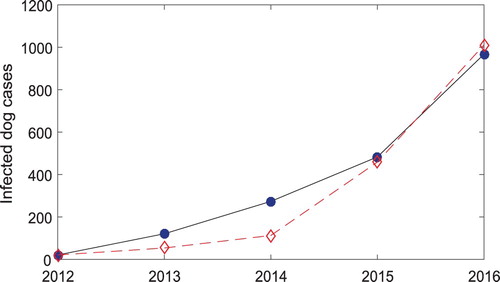
6. Calibration

Monthly GWD case data for dog populations were considered for the period 2012 to 2016 [6]. Our study focuses on the GWD outbreak in January 2012 to December 2016, a period when the disease prevalence decreased in humans but increased in dog population. We calibrate the copepod consumption rates by humans, ${\beta }_h$, and dogs, ${\beta }_d$, to match the GWD cases in Chad. We fit the model (1(1) $\begin{array}{rl}\frac{d{S}_h}{dt}& ={\pi }_h-{\beta }_h\left(\frac{I_c}{{\phi }_c}\right)S_h-{\mu }_h{S}_h+{\eta }_h(I_h^1+I_h^2),\\ \frac{d{E}_h^1}{dt}& =(1-\rho ){\beta }_h\left(\frac{I_c}{{\phi }_c}\right)S_h-({\mu }_h+{\gamma }_h)E_h^1,\\ \frac{d{E}_h^2}{dt}& =\rho {\beta }_h\left(\frac{I_c}{{\phi }_c}\right)S_h-({\mu }_h+{\gamma }_h)E_h^2,\\ \frac{d{I}_h^1}{dt}& ={\gamma }_h{E}_h^1-({\mu }_h+{\eta }_h)I_h^1,\\ \frac{d{I}_h^2}{dt}& ={\gamma }_h{E}_h^2-({\mu }_h+{\eta }_h)I_h^2,\\ \frac{d{S}_d}{dt}& ={\pi }_d-{\beta }_d\left(\frac{I_c}{{\phi }_c}\right)S_d-{\mu }_d{S}_d+{\eta }_d{I}_d,\\ \frac{d{E}_d}{dt}& ={\beta }_d\left(\frac{I_c}{{\phi }_c}\right)S_d-({\mu }_d+{\gamma }_d)E_d,\\ \frac{d{I}_d}{dt}& ={\gamma }_d{E}_d-({\mu }_d+{\eta }_d)I_d-c{I}_d,\\ \frac{d{S}_c}{dt}& =r{N}_c\left(1-\frac{N_c}{K_c}\right)-{\beta }_h\left(\frac{S_c}{{\phi }_c}\right)N_h-{\beta }_d\left(\frac{S_c}{{\phi }_c}\right)N_d-\delta \left(\frac{L}{{\phi }_L}\right)S_c-p{S}_c,\\ \frac{d{I}_c}{dt}& =\delta \left(\frac{L}{{\phi }_L}\right)S_c-{\beta }_h\left(\frac{I_c}{{\phi }_c}\right)N_h-{\beta }_d\left(\frac{I_c}{{\phi }_c}\right)N_d-({\mu }_c+p)I_c,\\ \frac{dL}{dt}& ={\lambda }_1{I}_h^1+{\lambda }_2{I}_d-{\mu }_{L}L-\delta \left(\frac{L}{{\phi }_L}\right)N_c.\end{array}$(1) ) without control interventions to equilibrium to yield the human GWD cases and the infected dog cases in the year 2012. The equilibrium solutions of the system (1(1) $\begin{array}{rl}\frac{d{S}_h}{dt}& ={\pi }_h-{\beta }_h\left(\frac{I_c}{{\phi }_c}\right)S_h-{\mu }_h{S}_h+{\eta }_h(I_h^1+I_h^2),\\ \frac{d{E}_h^1}{dt}& =(1-\rho ){\beta }_h\left(\frac{I_c}{{\phi }_c}\right)S_h-({\mu }_h+{\gamma }_h)E_h^1,\\ \frac{d{E}_h^2}{dt}& =\rho {\beta }_h\left(\frac{I_c}{{\phi }_c}\right)S_h-({\mu }_h+{\gamma }_h)E_h^2,\\ \frac{d{I}_h^1}{dt}& ={\gamma }_h{E}_h^1-({\mu }_h+{\eta }_h)I_h^1,\\ \frac{d{I}_h^2}{dt}& ={\gamma }_h{E}_h^2-({\mu }_h+{\eta }_h)I_h^2,\\ \frac{d{S}_d}{dt}& ={\pi }_d-{\beta }_d\left(\frac{I_c}{{\phi }_c}\right)S_d-{\mu }_d{S}_d+{\eta }_d{I}_d,\\ \frac{d{E}_d}{dt}& ={\beta }_d\left(\frac{I_c}{{\phi }_c}\right)S_d-({\mu }_d+{\gamma }_d)E_d,\\ \frac{d{I}_d}{dt}& ={\gamma }_d{E}_d-({\mu }_d+{\eta }_d)I_d-c{I}_d,\\ \frac{d{S}_c}{dt}& =r{N}_c\left(1-\frac{N_c}{K_c}\right)-{\beta }_h\left(\frac{S_c}{{\phi }_c}\right)N_h-{\beta }_d\left(\frac{S_c}{{\phi }_c}\right)N_d-\delta \left(\frac{L}{{\phi }_L}\right)S_c-p{S}_c,\\ \frac{d{I}_c}{dt}& =\delta \left(\frac{L}{{\phi }_L}\right)S_c-{\beta }_h\left(\frac{I_c}{{\phi }_c}\right)N_h-{\beta }_d\left(\frac{I_c}{{\phi }_c}\right)N_d-({\mu }_c+p)I_c,\\ \frac{dL}{dt}& ={\lambda }_1{I}_h^1+{\lambda }_2{I}_d-{\mu }_{L}L-\delta \left(\frac{L}{{\phi }_L}\right)N_c.\end{array}$(1) ) are found to be $\begin{array}{rl}& S_h=15550715,E_h^1=10.005,E_h^2=0,I_h^1=10,I_h^2=0,S_d=499767,\\ & E_d=21.0084,I_d=21,S_c=165911,I_c=33637,L=\mathrm{89.8079.}\end{array}$ GWD data are fitted using the built-in (MatLab, R2017a) simplex algorithm to minimize the sum of squares of the difference between simulated indicators and data. The minimization is conducted with 100 different starting points in parameter space, chosen using Latin Hypercube Sampling, to ensure consistency and uniqueness of the parameter estimates. The estimated parameters are given in Table 1. Further, to match the infected dog cases over the period 2012–2016, we estimated the dog recruitment rate, ${\pi }_d$, and copepod consumption rate by dogs, ${\beta }_d$, using the Nonlinear Least Squares fitting routine lsqnonlin in the optimization tool box (MATLAB, R2017a). The fitting is displayed in Figure 5. The initial conditions are chosen as equilibrium solutions.

Figure 5. Plots of the observed infected dog cases and the fitted model solution. The dashed line is the observed data and the solid line is the model solution.

7. Sensitivity analysis

In comparison to the effects of simply varying the parameters to look at the outcome of the model, the techniques of sensitivity analysis are mathematically more sophisticated. In the present case, we use a global sensitivity analysis techniques following Marino et al. [21]. To see the effect of the control related parameters, ρ, c and p, and the copepods consumption rates by humans (${\beta }_h$) and dogs (${\beta }_d$), we compute partial rank correlation coefficients (PRCCs) between these parameters with respect to basic reproduction number ($R_0$). The rest of the parameter values are the same as in Table 1. Nonlinear and monotone relationships were observed for the parameters under consideration and the response parameter $R_0$. We draw 1000 samples from the biologically feasible regions of the parameters of interest using Latin Hypercube Sampling (LHS). The bar diagram of the PRCC values is depicted in Figure 6.

Figure 6. This figure depicts the PRCC for the parameters ρ, c, p, ${\beta }_h$ and ${\beta }_d$ influencing the reproduction number, $R_0$, with two stars on the top of the bars showing parameters that have PRCC statistically different from zero. A lower value of $R_0$ is preferable since it enhances the possibility of eradication of GWD. Therefore, above all, an increase in the parameter ${\beta }_d$ must be prevented by all means, while an increase in the parameters c and p should instead be favoured.

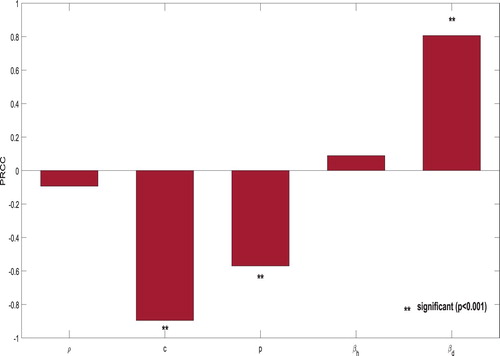
PRCC values of these parameters suggest that the copepods consumption rates by dogs (${\beta }_d$) has the maximum positive correlation with $R_0$ while the isolation rate of infected dogs (c) has the maximum negative correlation with $R_0$. The clearance rate of copepods (p) has significant negative correlation with $R_0$. It is well known that a low value of $R_0$ increases the likelihood of eradicating GWD. Therefore, it is highly improbable that they change in the direction that one would like, but any external measure that reduces ${\beta }_d$ and increases c and p should, therefore, be considered in order to eliminate GWD from the community.

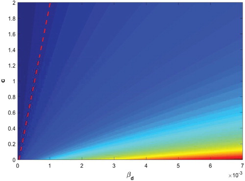
Furthermore, to investigate the effect of the most sensitive parameters on $R_0$, we draw the contour plot of $R_0$ with respect to the two controllable parameters ${\beta }_d$ and c for the model (1(1) $\begin{array}{rl}\frac{d{S}_h}{dt}& ={\pi }_h-{\beta }_h\left(\frac{I_c}{{\phi }_c}\right)S_h-{\mu }_h{S}_h+{\eta }_h(I_h^1+I_h^2),\\ \frac{d{E}_h^1}{dt}& =(1-\rho ){\beta }_h\left(\frac{I_c}{{\phi }_c}\right)S_h-({\mu }_h+{\gamma }_h)E_h^1,\\ \frac{d{E}_h^2}{dt}& =\rho {\beta }_h\left(\frac{I_c}{{\phi }_c}\right)S_h-({\mu }_h+{\gamma }_h)E_h^2,\\ \frac{d{I}_h^1}{dt}& ={\gamma }_h{E}_h^1-({\mu }_h+{\eta }_h)I_h^1,\\ \frac{d{I}_h^2}{dt}& ={\gamma }_h{E}_h^2-({\mu }_h+{\eta }_h)I_h^2,\\ \frac{d{S}_d}{dt}& ={\pi }_d-{\beta }_d\left(\frac{I_c}{{\phi }_c}\right)S_d-{\mu }_d{S}_d+{\eta }_d{I}_d,\\ \frac{d{E}_d}{dt}& ={\beta }_d\left(\frac{I_c}{{\phi }_c}\right)S_d-({\mu }_d+{\gamma }_d)E_d,\\ \frac{d{I}_d}{dt}& ={\gamma }_d{E}_d-({\mu }_d+{\eta }_d)I_d-c{I}_d,\\ \frac{d{S}_c}{dt}& =r{N}_c\left(1-\frac{N_c}{K_c}\right)-{\beta }_h\left(\frac{S_c}{{\phi }_c}\right)N_h-{\beta }_d\left(\frac{S_c}{{\phi }_c}\right)N_d-\delta \left(\frac{L}{{\phi }_L}\right)S_c-p{S}_c,\\ \frac{d{I}_c}{dt}& =\delta \left(\frac{L}{{\phi }_L}\right)S_c-{\beta }_h\left(\frac{I_c}{{\phi }_c}\right)N_h-{\beta }_d\left(\frac{I_c}{{\phi }_c}\right)N_d-({\mu }_c+p)I_c,\\ \frac{dL}{dt}& ={\lambda }_1{I}_h^1+{\lambda }_2{I}_d-{\mu }_{L}L-\delta \left(\frac{L}{{\phi }_L}\right)N_c.\end{array}$(1) ), Figure 7. The contour plot shows that the epidemic potential of GWD can be taken to below unity through interventions and aggressive efforts.

Figure 7. Contour plot of the basic reproduction number, $R_0$, in terms of two controllable parameters: ${\beta }_d$ (copepods consumption rate by dogs) and c (isolation rate of infected dogs). The dashed line represents $R_0=1$.

8. Impact of control interventions

In this section, we discuss the reduction in infected humans by varying the control parameters; percentage of aware human (ρ), isolation rate of infected dogs (c) and copepod removal rate (p).

(A) Increasing the percentage of aware humans: Health related education relevant to GWD is given to ensure that most of the individuals in the endemic region adopt behavioural practices that can prevent and interrupt the transmission cycle. Practices include voluntary reporting of GWD cases and knowledge of the reward scheme, prevention of patients from entering drinking-water bodies, regular use of drinking water from improved water sources and, in the absence of such sources, filtering water before drinking [4]. Although filtration appears to be easy and effective, challenges remain in individual and household compliance with straining all unsafe drinking water before consumption and, more importantly, in the agricultural fields or when travelling. In below poverty regions, face-to-face communication appeared to have been the most significant strategy for disseminating messages [27]. Behavioural changes have to be brought about in the community to achieve the required impact, which remains a challenge [4]. By increasing the percentage of aware humans, we mean that most of the individuals are getting information about the disease and hence they will avoid contaminated water resources and infected individuals will not eject worm larvae to any water source. It is noted that even if the number of aware individuals is very high, say $\rho =0.9$, no noticeable changes in human infected with GWD is observed (Figure 8(c)). One possible reason behind this may be, no matter how large the aware individuals become, there is still a fraction ($1-\rho$) contributing to disease transmission. On the other hand, there will be endemicity in the human population, reservoir population and vector population because this strategy does not affect the dog and copepod population.

Figure 8. Impact of control interventions on the infected humans. First row p=0, c=0 and (a) $\rho =0.1$, (b) $\rho =0.5$ and (c) $\rho =0.9$. Second row p=0, $\rho =0$ and (d) c=0.3, (e) c=0.6 and (f) c=0.9. Third row c=0, $\rho =0$ and (g) p=0.7, (h) p=1.4 and (i) p=2.0.

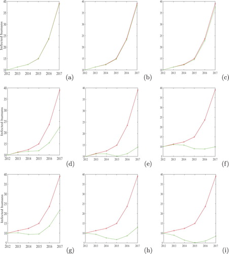
(B) Increasing the isolation rate of infected dogs: Eberhard et al. [11] pointed out that infection in dogs is serving as one of the major driving force sustaining transmission in Chad, that an aberrant life cycle involving a paratenic host common to people and dogs is occurring, and that the cases in humans are sporadic and incidental. Recently, Molyneux and Sankara [22] suggested that Ministries of Health with the support of WHO and the Carter Center, must focus on interrupting transmission by the vigorous pursuit of copepod control, the containment of human cases and dog infections and through the application of what we know works. Our results suggest that dog management, i.e., isolation of the infected dogs from the society, leads to a big reduction in infected human cases (Figure 8(e,f)). Therefore, this intervention is very important to achieve the complete eradication of GWD from Chad. Despite the high efficacy of case reduction, this control is very complicated to apply [11].

(C) Controlling the copepod: This intervention consists of killing the copepods by applying a chemical called temephos [11]. When applied to unsafe drinking-water sources on monthly basis, temephos is effective in killing the copepods. By applying this control, we can effectively reduce the contact rate of Guinea worm with humans as well as dogs. Numerically, we checked the effect of copepod control at various levels (Figure 8(g–i)). One can easily find that this intervention can effectively reduce the number of infected humans. Note that intervention (B) appears to be slightly better than this control.

(D) Comparison of cases in 2017 after applying the control interventions: A provisional total of 26 cases of GWD has been reported in 2017 among which a total of 12 apparent cases were detected in Ethiopia and 14 cases in Chad [14]. To compare the cases in 2017, we have computed the number of cases in 2017 with control interventions (see, Figure 9). Due to the application of various control interventions in Chad, it is observed that the model (1(1) $\begin{array}{rl}\frac{d{S}_h}{dt}& ={\pi }_h-{\beta }_h\left(\frac{I_c}{{\phi }_c}\right)S_h-{\mu }_h{S}_h+{\eta }_h(I_h^1+I_h^2),\\ \frac{d{E}_h^1}{dt}& =(1-\rho ){\beta }_h\left(\frac{I_c}{{\phi }_c}\right)S_h-({\mu }_h+{\gamma }_h)E_h^1,\\ \frac{d{E}_h^2}{dt}& =\rho {\beta }_h\left(\frac{I_c}{{\phi }_c}\right)S_h-({\mu }_h+{\gamma }_h)E_h^2,\\ \frac{d{I}_h^1}{dt}& ={\gamma }_h{E}_h^1-({\mu }_h+{\eta }_h)I_h^1,\\ \frac{d{I}_h^2}{dt}& ={\gamma }_h{E}_h^2-({\mu }_h+{\eta }_h)I_h^2,\\ \frac{d{S}_d}{dt}& ={\pi }_d-{\beta }_d\left(\frac{I_c}{{\phi }_c}\right)S_d-{\mu }_d{S}_d+{\eta }_d{I}_d,\\ \frac{d{E}_d}{dt}& ={\beta }_d\left(\frac{I_c}{{\phi }_c}\right)S_d-({\mu }_d+{\gamma }_d)E_d,\\ \frac{d{I}_d}{dt}& ={\gamma }_d{E}_d-({\mu }_d+{\eta }_d)I_d-c{I}_d,\\ \frac{d{S}_c}{dt}& =r{N}_c\left(1-\frac{N_c}{K_c}\right)-{\beta }_h\left(\frac{S_c}{{\phi }_c}\right)N_h-{\beta }_d\left(\frac{S_c}{{\phi }_c}\right)N_d-\delta \left(\frac{L}{{\phi }_L}\right)S_c-p{S}_c,\\ \frac{d{I}_c}{dt}& =\delta \left(\frac{L}{{\phi }_L}\right)S_c-{\beta }_h\left(\frac{I_c}{{\phi }_c}\right)N_h-{\beta }_d\left(\frac{I_c}{{\phi }_c}\right)N_d-({\mu }_c+p)I_c,\\ \frac{dL}{dt}& ={\lambda }_1{I}_h^1+{\lambda }_2{I}_d-{\mu }_{L}L-\delta \left(\frac{L}{{\phi }_L}\right)N_c.\end{array}$(1) ) can well reflect the 2017 cases of GWD for certain values of control parameters.

Figure 9. Impact of controls on the predicted cases in 2017: (a) p=0 and c=0, (b) p=0 and $\rho =0$ and (c) c=0 and $\rho =0$. The solid black line represents the provisional number of cases between 1 January and 31 October 2017 [14].

Further, we evaluated the effects of all controls in Figure 10(a–c). We plotted the number of new GWD cases by varying the control parameters, ρ, c and p. Looking at the figures, it is evident that copepod control is the most effective way to reduce human infections. The percentage of reduction in infected humans due to the application of individual control strategies are given in Table 2. Form the table, it is reinforced that the isolation rate of infected dogs is most effective in terms of case reduction of GWD.

Figure 10. Impact of controls on the predicted cases in 2018: (a) p=0 and c=0, (b) p=0 and $\rho =0$ and (c) c=0 and $\rho =0$. The contour plots on the second row correspond to the combined effects of control interventions: (d) p=0, (e) $\rho =0$ and (f) c=0.

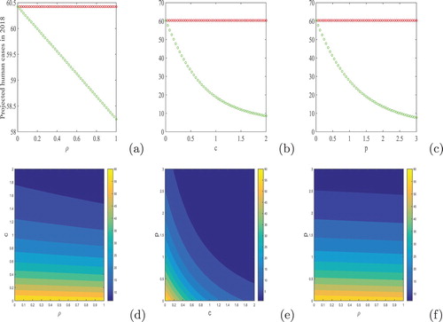
Table 2. Percentage reduction in infected humans.

Control measures	Percentage reduction in infected humans
c=0, p=0, $\rho =0.1$	0.4129
c=0, p=0, $\rho =0.5$	2.0670
c=0, p=0, $\rho =0.9$	3.7250
$\rho =0$, p=0, c=0.5	42.6594
$\rho =0$, p=0, c=1.0	63.9320
$\rho =0$, p=0, c=1.5	74.6585
c=0, $\rho =0$, p=0.7	44.3670
c=0, $\rho =0$, p=1.4	66.6921
c=0, $\rho =0$, p=2.1	78.4134

(E) Combination of control interventions: We investigate the effect of combination strategies namely; (A,B), (B,C) and (A,C) by simulating the number of new GWD cases in 2018 (see, Figure 10(d–f)). The contour lines represent the infected human populations. It can be inferred from the contour plots that the combination strategy (B,C) is the most effective in comparison to the others.

9. Discussion

In this paper, we proposed and analysed a mathematical model for GWD in order to give some insights into the eradication process of GWD in Chad. To estimate the important parameters of the model (1(1) $\begin{array}{rl}\frac{d{S}_h}{dt}& ={\pi }_h-{\beta }_h\left(\frac{I_c}{{\phi }_c}\right)S_h-{\mu }_h{S}_h+{\eta }_h(I_h^1+I_h^2),\\ \frac{d{E}_h^1}{dt}& =(1-\rho ){\beta }_h\left(\frac{I_c}{{\phi }_c}\right)S_h-({\mu }_h+{\gamma }_h)E_h^1,\\ \frac{d{E}_h^2}{dt}& =\rho {\beta }_h\left(\frac{I_c}{{\phi }_c}\right)S_h-({\mu }_h+{\gamma }_h)E_h^2,\\ \frac{d{I}_h^1}{dt}& ={\gamma }_h{E}_h^1-({\mu }_h+{\eta }_h)I_h^1,\\ \frac{d{I}_h^2}{dt}& ={\gamma }_h{E}_h^2-({\mu }_h+{\eta }_h)I_h^2,\\ \frac{d{S}_d}{dt}& ={\pi }_d-{\beta }_d\left(\frac{I_c}{{\phi }_c}\right)S_d-{\mu }_d{S}_d+{\eta }_d{I}_d,\\ \frac{d{E}_d}{dt}& ={\beta }_d\left(\frac{I_c}{{\phi }_c}\right)S_d-({\mu }_d+{\gamma }_d)E_d,\\ \frac{d{I}_d}{dt}& ={\gamma }_d{E}_d-({\mu }_d+{\eta }_d)I_d-c{I}_d,\\ \frac{d{S}_c}{dt}& =r{N}_c\left(1-\frac{N_c}{K_c}\right)-{\beta }_h\left(\frac{S_c}{{\phi }_c}\right)N_h-{\beta }_d\left(\frac{S_c}{{\phi }_c}\right)N_d-\delta \left(\frac{L}{{\phi }_L}\right)S_c-p{S}_c,\\ \frac{d{I}_c}{dt}& =\delta \left(\frac{L}{{\phi }_L}\right)S_c-{\beta }_h\left(\frac{I_c}{{\phi }_c}\right)N_h-{\beta }_d\left(\frac{I_c}{{\phi }_c}\right)N_d-({\mu }_c+p)I_c,\\ \frac{dL}{dt}& ={\lambda }_1{I}_h^1+{\lambda }_2{I}_d-{\mu }_{L}L-\delta \left(\frac{L}{{\phi }_L}\right)N_c.\end{array}$(1) ), we fit the system to equilibrium and found the consumption rates of copepods by humans, ${\beta }_h$, and dogs, ${\beta }_d$. Further, to match the infected dog cases in 2012–2016, we estimated the recruitment rate of dogs, ${\pi }_d$, and the copepods consumption rate by dogs, ${\beta }_d$. To observe the effect of the control parameters and copepods consumption rates by humans and dogs on the basic reproduction number, we performed global sensitivity analysis which gives us a clear idea of the important control parameters. The PRCCs of $R_0$ to these parameters show that the most critical parameter impacting $R_0$ is the copepods consumption rate by dogs, ${\beta }_d$. In addition, the isolation rate of infected dogs, c, and the clearance rate of copepods, p, have significant impacts on $R_0$ and consequently on the control of GWD. We conclude that external measures decreasing $R_0$ should be encouraged.

Numerically we investigated effects of the three control parameters, ρ, c and p, on the infected human cases. It is shown that the cases in 2017 can be predicted by the model for some values of the control parameters. We found that isolation of infected dogs is the most effective as compared to other controls, Figure 8. The isolation of infected dogs requires a huge effort and sometimes it is hard to contain all of the infected dogs. Keeping this in mind, the clearance of copepods is a much simpler strategy to apply whose effect is very close to the effect of isolating dogs (see, Table 2). In addition, we studied the combined effects of the control strategies by predicting the number of infected human cases in 2018. The first three panels of Figure 10 show the similar kind of results. Figure 10 gives a clearer picture that the combination of isolating infected dogs and clearing the copepods leads to the reduction of the largest number of cases. Implies that this combination strategy will take huge effort as there may be difficulties in identifying which sources of surface water are potentially contaminated and need to be treated. In summary, to achieve the permanent eradication of worldwide GWD cases, the infections in dog population must be reduced. The affected countries should be effectively financed to isolate infected dogs and treat the contaminated ponds with temephos. We recommend that the health-care agencies must focus on containing the infected dogs as well as treating ponds.

Disclosure statement

The authors declare that they have no conflicts of interest.

ORCID

Indrajit Ghosh  http://orcid.org/0000-0002-0492-2948

Additional information

Funding

Indrajit Ghosh was supported by the Senior Research Fellowship from University Grants Commission, Government of India. P. K. Tiwari is thankful to National Board of Higher Mathematics, Department of Atomic Energy, Government of India for providing financial support in form of Post Doctoral Fellowship. The funders had no role in study design, data collection and analysis, decision to publish or preparation of the manuscript. This work was also supported by Division of Mathematical Sciences [1515661].

References

- A. Abate, A. Tiwari, and S. Sastry, Box invariance in biologically-inspired dynamical systems, Automatica 45 (2009), pp. 1601–1610.
- I.A. Adetunde, The epidemiology of Guinea Worm Infection in Tamale district, in the Northern Region of Ghana, J. Modern Math. Stat. 2 (2008), pp. 50–54.
- E. Beltrami and T.O. Carroll, Modeling the role of viral disease in recurrent phytoplankton blooms, J. Math. Biol. 32 (1994), pp. 857–863.
- G. Biswas, D.P. Sankara, J. Agua-Agum, and A. Maiga, Dracunculiasis (Guinea worm disease): Eradication without a drug or a vaccine, Phil. Trans. R. Soc. B 368 (2013). doi:10.1098/rstb.2012.0146.
- S. Cairncross, R. Muller, and N. Zagaria, Dracunculiasis (Guinea worm disease) and the eradication initiative, Clin. Microbiol. Rev. 15 (2002), pp. 223–246.
- E. Callaway, Dogs thwart end to Guinea worm, Nature 529 (2016), pp. 10–11.
- F. Carlotti and S. Nival, Moulting and mortality rates of copepods related to age within stage: Experimental results, Mar. Ecol. Prog. Ser. 84 (1992), pp. 235–243.
- C. Castillo-Chavez and B. Song, Dynamical models of tuberculosis and their applications, Math. Biosci. Eng. 1 (2004), pp. 361–404.
- C. Castillo-Chavez, Z. Feng, and W. Huang, On the computation of R0 and its role on global stability, in Mathematical Approaches for Emerging and Reemerging Infectious Diseases: An Introduction 1, Springer-Verlag, New York, 2002, p. 229.
- Centers for Disease Control and Prevention. DPDx – Laboratory identification of parasitic diseases of public health concern, (2016). Available at https://www.cdc.gov/dpdx/dracunculiasis/.
- M.L. Eberhard, E. Ruiz-Tiben, D.R. Hopkins, C. Farrell, F. Toe, A. Weiss, Jr., P.C. Withers, M.H.Jenks, E.A. Thiele, J.A. Cotton, and Z. Hance, The peculiar epidemiology of dracunculiasis in Chad, Amer. J. Trop. Med. Hyg. 90(1) (2014), pp. 61–70.
- H.I. Freedman and J.W.H. So, Global stability and persistence of simple food chains, Math. Biosci.76 (1985), pp. 69–86.
- Global Health Workforce Alliance. Available at http://www.who.int/workforcealliance/countries/tcd/en/.
- Guinea worm outbreak in Ethiopia, Public Health Service, Centers for Disease Control and Prevention. Available at https://www.cartercenter.org/resources/pdfs/news/health_publications/guinea_worm/wrap-up/251.pdf.
- J.K. Hale, Ordinary Differential Equations, Wiley-Inscence, New York, 1969.
- D.L. Heymann, Control of Communicable Diseases Manual, 18th ed., APHA, Washington, DC, 2004.
- D.R. Hopkins, E. Ruiz-Tiben, A. Weiss, P. Withers Jr., M. Eberhard, and S. Roy, Dracunculiasis eradication: And now South Sudan, Amer. J. Trop. Med. Hyg. 89 (2013), pp. 5–10.
- P.J. Hotez, E. Ottesen, A. Fenwick, and D. Molyneaux, The neglected tropical diseases: The ancient afflictions of stigma and poverty and the prospects for their control and elimination, in Hot Topics in Infection and Immunity in Children III, A.J. Pollard and A. Finn, eds., Kluwer Academic/Plenum Publishers, New York, 2006.
- M.K. Kindhauser, Communicable Diseases 2002: Global Defence Against the Infectious Disease Threat, WHO, Geneva, Switzerland, 2003.
- K. Link and D. Victor, Guinea worm disease (Dracunculiasis): Opening a mathematical can of worms, M.Sc. Thesis, Bryn Mawr College, Pennsylvania, USA, 2012.
- S. Marino, I.B. Hogue, C.J.R. Ray, and D.E. Kirschner, A methodology for performing global uncertainty and sensitivity analysis in systems biology, J. Theor. Biol. 254 (2008), pp. 178–196.
- D. Molyneux and D.P. Sankara, Guinea worm eradication: Progress and challenges – should we beware of the dog? PLoS Negl. Trop. Dis. 11(4) (2017), p. e0005495.
- R. Muller, Dracunculus and dracunculiasis, Adv. Parasitol. 9 (1971), pp. 73–151.
- R. Muller, Guinea worm disease: Epidemiology, control, and treatment, Bull. World Health Org. 57(5) (1979), pp. 683–689.
- L. Perko, Differential Equations and Dynamical Systems. 3rd ed. Springer-Verlag, New York, 2000.
- R.J. Smith?, P. Cloutier, J. Harrison, and A. Desforges, A mathematical model for the eradication of Guinea worm disease, in Understanding the Dynamics of Emerging and Re-Emerging Infectious Diseases Using Mathematical Models, Transworld Research Network, Kerala, 2012, pp. 133–156.
- A. Tayeh, S. Cairncross, and G.H. Maude, The impact of health education to promote cloth filters on dracunculiasis prevalence in the northern region, Ghana, Soc. Sci. Med. 43 (1996), pp. 1205–1211.
- United Nation Report: Population Division, Department of Economic and Social Affairs, World Population Prospects: The 2012 revision.
- P. van den Driessche and J. Watmough, Reproduction numbers and sub-threshold endemic equilibria for compartmental models of disease transmission, Math. Biosci. 180 (2002), pp. 29–48.
- X. Wang and J. Lou, Two dynamic models about rabies between dogs and human, J. Biol. Syst. 16(4) (2008), pp. 519–529.
- World Health Organization, Dracunculiasis eradication in Uzbekistan: Country report, WHO/CDS/CEE/DRA/99.9. WHO, Geneva, 1998.