Efficacy of control measures in the control of Ebola, Liberia 2014–2015

ABSTRACT

The largest outbreak of Ebola to date is the 2014 West Africa Ebola outbreak, with more than 10,000 cases and over 4000 deaths reported in Liberia alone. To control the spread of the outbreak, multiple interventions were implemented: identification and isolation of cases, contact tracing, quarantining of suspected contacts, proper personal protection, safely conducted burials, improved education, social awareness and individual protective measures. Devising rigorous methodologies for the evaluation of the effectiveness of the control measures implemented to stop an outbreak is of paramount importance. In this paper, we evaluate the effectiveness of the 2014 Ebola outbreak interventions. We rely on model selection to determine the best model that explains the 2014 Ebola outbreak data in Liberia which is the simplest model with a social distancing term. We couple structural and practical identifiability analysis with the computation of confidence intervals to pinpoint the uncertainty in the parameter estimations. Finally, we evaluate the efficacy of control measures using the Ebola model with social distancing. Among all the control measures, we find that social distancing had the most impact on the control of the 2014 Ebola epidemic in Libreria followed by isolation and quarantining.

KEYWORDS:

• Ebola
• outbreak
• mathematical models
• differential equations
• Akaike Information Criterion
• reproduction number
• control measures
• mathematical epidemiology

AMS SUBJECT CLASSIFICATIONS:

• 92D30
• 92D40

1. Introduction

Emerging infectious diseases present challenge to public health every day. Mathematical models can facilitate combating these diseases by projecting potential cases, estimating key parameters of the outbreak, evaluating and optimizing control strategies. The use of mathematical modelling in the control of deadly diseases, such as the Ebola Viral Diseases (Ebola) outbreak of 2014–2015 in West Africa [5], has become wide spread, and numerous models have been created targeting different objectives.

Early in the West Africa Ebola epidemic, a number of mechanistic models were developed, fitted to data and used to predict cases or estimate the reproduction number ${\mathcal{R}}_0$. Chretien et al. [9] reviewed the models in 66 articles and found that almost all of them estimated ${\mathcal{R}}_0$ and many of them made projections. The study concluded that articles that estimated ${\mathcal{R}}_0$ ‘using the same data sources at about the same time reported varied results ', a conclusion that is hardly surprising, given the variety of modelling approaches, methods to compute ${\mathcal{R}}_0$, uncertainty in the data and a wide-spread un-identifiability of the models. Ignoring the cumulative incidence [13], which in essence codes additional information about the data, further decreases our ability to make estimates that give a coherent picture, potentially useful for public health officials.

The Ebola epidemic in West Africa is over and now is the time to understand the key implications of modelling emerging outbreaks. One of the lessons learned is that not all diseases develop the same in their early (and perhaps more advanced) stages. Chowell et al. [7] suggest that the incidence growth for Ebola in West Africa, particularly on local level, was not exponential, as it might be in an outbreak of influenza, but more reminiscent of the subexponential growth of HIV in the US. This is probably due to public awareness and social distancing. We also find that models with mass action or standard incidence, which comprise a large percentage of the models used, are not adequate to explain the full data sets not only for the Ebola outbreak but also for the worldwide prevalence and death of HIV [22]. For this reason, we use here a modified incidence with an exponential term, incorporated to depict social distancing as the outbreak unfolds. The role of human behaviour in the development and control of infectious disease outbreak cannot be underestimated [15], yet this key component has been included little in models of Ebola outbreak in West Africa.

Most of the models developed for the 2014–2015 Ebola outbreak are based on earlier models of outbreaks from 1995 to 2000 in Congo, Uganda and the Philippines [8,18]. Early and newer models were used for parameter estimation and computation of ${\mathcal{R}}_0$ without investigation of their identifiability. The computation of the confidence intervals quantifies the uncertainty involved in our estimates but these intervals will be different if the model is identifiable in the first place. Only recently, the identifiability of epidemic models is beginning to be investigated [10,24] and these results have not been connected to the confidence intervals.

Several papers address efficacies of interventions, some focusing on specific measures, such as contact tracing [1] or combinations such as isolation, contact tracing and supportive treatment [23]. Other modelling efforts take a more comprehensive view and investigate the impact of multiple control scenarios [20,21]. In general, there are two main ways to incorporate interventions. In the first one, interventions are envisioned as a change in the parameters of a basic model [20], while in the second one interventions are incorporated as the part of the model [21]. The first approach creates difficulties in evaluating which parameter is affected by which control measure and how [20], while the second leads to a much more complex model, holding a greater potential of not being identifiable [21]. Evaluating the efficacies of multiple control measures during the Ebola outbreak, we introduce a mixed approach that collapses a model incorporating multiple interventions to our simple baseline model without interventions but in the process we can evaluate which parameters are affected and how.

In this study, the Ebola outbreak data are collected from the World Health Organization (WHO) reports published at its website [28]. Using the WHO data, we perform model selection on eight Ebola outbreak models, clustered into two groups – depending on whether they incorporate or not a social distancing term. The group without the social distancing term consists of a basic model, a model with exposed class, a model with a quarantined class and a model with both exposed and quarantined class. The second group consists of the same four models but each incorporating a social distancing term. We then use the Akaike Information Criterion (AIC) to choose the model that explains the WHO data best, thus contrasting models with various components: properties of the disease, interventions and/or human behaviour. Once we select the best model, we address the question of the well-posedness of the parameter estimation problem, termed as structural identifiability of the mathematical model. Structural identifiability studies whether the parameters of the model can be recovered from the observed state (output) under ideal conditions such as noise-free data and error-free computation. We analyse the structural identifiability of the selected model without the social distancing term and the practical identifiability of the selected Ebola model considered in this study. We then evaluate the impact of the control measures implemented for the Ebola outbreak by applying the sensitivity methods to rank the public health interventions (education, quarantining, isolation, safe burial and social distancing).

The paper is organized as follows: the Ebola outbreak models are introduced in Section 2 and the AIC criterium is used to compare these models against the data. The structural and practical identifiability of the best fitted models with and without social distancing are performed in Section 3. Confidence intervals for the estimated parameters are also computed. Based on the results of Section 3, in Section 4, the impact of the control measures is evaluated. We then summarize and discuss the results in Section 5.

2. Model selection for Ebola

In this section, we introduce the selection of ordinary differential equation models for Ebola. Ebola is transmitted through bodily fluids, so the main path of transmission is direct [4]. There are two possible outcomes of Ebola infection: death and recovery. References suggest that recovered individuals may continue to be infectious for about 7 weeks after recovery [29]. After 7 weeks, recovered individuals are assumed to be no longer infectious. To encompass the specificity of Ebola, we split the recovered class into two subclasses: recovered but infectious and recovered but no longer infectious. Furthermore, recently deceased individuals who suffered from Ebola continue to be infectious for as long as the body secretes fluids [4]. We incorporate this into the models by allowing deceased individuals to transmit the disease. To introduce the first model, let S be the number of susceptible individuals, I be the number of infectious individuals, R be the number of recovered but still infectious individuals, $R_m$ be the number of removed individuals including the recovered and deceased individuals who are no longer infectious, and D be the number of individuals who died from Ebola. The dependent variables are summarized in Table 1.

Table 1. List of state variables used in Ebola models.

Notation	Meaning
$S\left(t\right)$	Number of susceptible individuals at time t
$E\left(t\right)$	Number of exposed individuals at time t
$Q\left(t\right)$	Number of isolated individuals at time t
$I\left(t\right)$	Number of infected individuals at time t
$R\left(t\right)$	Recovered but still infectious individuals at time t
$R_m\left(t\right)$	Removed class including the recovered individuals who are not infectious at time t
$D\left(t\right)$	Number of deceased individuals (who continue to be infectious) at time t

Ebola is typically modelled as an outbreak disease, and these models do not contain natural human birth and death due to the short duration of the outbreak. The first mathematical model we consider for Ebola takes the following form, (1) $\mathrm{Model}1\left(M_1\right):\left\{\begin{array}{l}\frac{\mathrm{d}S}{\mathrm{d}t}=-\beta S(I+q_{1}R+q_{2}D),\\ \frac{\mathrm{d}I}{\mathrm{d}t}=\beta S(I+q_{1}R+q_{2}D)-(\gamma +\alpha )I,\\ \frac{\mathrm{d}R}{\mathrm{d}t}=\gamma I-\eta R,\\ \frac{\mathrm{d}D}{\mathrm{d}t}=\alpha I-\nu D,\\ \frac{\mathrm{d}{R}_m}{\mathrm{d}t}=\eta R+\nu D,\end{array}\right.$(1) where β is the transmission rate for Ebola, α is the disease-induced death rate, γ is the recovery rate, η is the rate of progression from infectious to non-infectious recovery, $q_1$ is the coefficient of reduction or enhancement of transmission of recovered individuals and $q_2$ is the coefficient of reduction or enhancement of transmission of dead individuals. The relative contribution to the infection of recovered individuals in class R and the deceased individuals in class D is not known.

We introduce total of eight models for Ebola. The parameters for these eight models are summarized in Table 2. Next, we introduce the nested submodels of the global model ($M_8$).

Table 2. List of parameters in Ebola models.

Notation	Meaning
β	Transmission rate for Ebola
α	Disease-induced mortality of infected individuals
γ	Recovery rate of infected individuals
η	Rate of progression from infectious to non-infectious recovery
$q_1$	Coefficient of reduction or enhancement of transmission of recovered individuals
$q_2$	Coefficient of reduction or enhancement of transmission of deceased individuals
σ	Rate of becoming infectious for exposed individuals
ξ	Isolation rate of infected individuals
${\alpha }_2$	Disease-induced mortality of isolated individuals
${\gamma }_2$	Recovery rate of isolated individuals
ν	Rate of progression of deceased to removed class
κ	Rate of social distancing

In moving to more complicated models, we consider the stages of infection and control measures implemented for Ebola outbreak. Many models of Ebola currently used to describe the unprecedented outbreak in West Africa have an exposed and isolated classes [3,14,25]. Besides the first model $M_1$, we introduce three more models: one that includes an exposed class, $E\left(t\right)$, ($M_2$), one that includes an isolated class, $Q\left(t\right)$, ($M_3$), and one that includes both an exposed and an isolated class ($M_4$). The second model, $M_2$, which includes the exposed class is given by the following equations: (2) $M_2:\left\{\begin{array}{l}\frac{\mathrm{d}S}{\mathrm{d}t}=-\beta S(I+q_{1}R+q_{2}D),\\ \frac{\mathrm{d}E}{\mathrm{d}t}=\beta S(I+q_{1}R+q_{2}D)-\sigma E,\\ \frac{\mathrm{d}I}{\mathrm{d}t}=\sigma E-(\alpha +\gamma )I,\\ \frac{\mathrm{d}R}{\mathrm{d}t}=\gamma I-\eta R,\\ \frac{\mathrm{d}D}{\mathrm{d}t}=\alpha I-\nu D,\\ \frac{\mathrm{d}{R}_m}{\mathrm{d}t}=\eta R+\nu D.\end{array}\right.$(2) Here the newly infected individuals move into an exposed class, and then they progress to the infectious class. All other classes are as in $M_1$ (1(1) $\mathrm{Model}1\left(M_1\right):\left\{\begin{array}{l}\frac{\mathrm{d}S}{\mathrm{d}t}=-\beta S(I+q_{1}R+q_{2}D),\\ \frac{\mathrm{d}I}{\mathrm{d}t}=\beta S(I+q_{1}R+q_{2}D)-(\gamma +\alpha )I,\\ \frac{\mathrm{d}R}{\mathrm{d}t}=\gamma I-\eta R,\\ \frac{\mathrm{d}D}{\mathrm{d}t}=\alpha I-\nu D,\\ \frac{\mathrm{d}{R}_m}{\mathrm{d}t}=\eta R+\nu D,\end{array}\right.$(1) ). Next we introduce a model with isolated class but without an exposed class. The model $M_3$ which includes the isolated class is given as follows. (3) $M_3:\left\{\begin{array}{l}\frac{\mathrm{d}S}{\mathrm{d}t}=-\beta S(I+q_{1}R+q_{2}D),\\ \frac{\mathrm{d}I}{\mathrm{d}t}=\beta S(I+q_{1}R+q_{2}D)-(\alpha +\gamma +\xi )I,\\ \frac{\mathrm{d}Q}{\mathrm{d}t}=\xi I-({\alpha }_2+{\gamma }_2)Q,\\ \frac{\mathrm{d}R}{\mathrm{d}t}=\gamma I+{\gamma }_{2}Q-\eta R,\\ \frac{\mathrm{d}D}{\mathrm{d}t}=\alpha I-\nu D,\\ \frac{\mathrm{d}{R}_m}{\mathrm{d}r}=\eta R+{\alpha }_{2}Q+\nu D.\end{array}\right.$(3) Since the supportive care reflects positively on the disease survivability, the isolated individuals recover and die from the disease at different rates than infectious individuals. The next model $M_4$ includes both exposed and isolated classes and is given by the following equations: (4) $M_4:\left\{\begin{array}{l}\frac{\mathrm{d}S}{\mathrm{d}t}=-\beta S(I+q_{1}R+q_{2}D),\\ \frac{\mathrm{d}E}{\mathrm{d}t}=\beta S(I+q_{1}R+q_{2}D)-\sigma E,\\ \frac{\mathrm{d}I}{\mathrm{d}t}=\sigma E-(\alpha +\gamma +\xi )I,\\ \frac{\mathrm{d}Q}{\mathrm{d}t}=\xi I-({\alpha }_2+{\gamma }_2)Q,\\ \frac{\mathrm{d}R}{\mathrm{d}t}=\gamma I+{\gamma }_{2}Q-\eta R,\\ \frac{\mathrm{d}D}{\mathrm{d}t}=\alpha I-\nu D,\\ \frac{\mathrm{d}{R}_m}{\mathrm{d}t}=\eta R+{\alpha }_{2}Q+\nu D.\end{array}\right.$(4) In the first four models ($M_1,M_2,M_3,M_4$), the new incidences are modelled by ‘mass-action’ term which states that the number of contacts and the probability that the contact will result in transmission of the infection is assumed in a homogenous population. Thus the behavioural influences of individuals towards an emerging Ebola outbreak are not considered. We continue by including behavioural influences in modelling new incidences. Behaviour epidemiology of infectious diseases is an emerging subdiscipline that studies the complex interaction between the human behaviour in response to an infectious disease and the impact of that behaviour on the disease characteristics and dynamics. Behaviour modifications are typically incorporated into mathematical models through including additional classes that signify alternative behaviour [15]. In this article, we use a different, more parsimonious approach by incorporating social distancing as an exponential term modifying transmission. Influence of social distancing in the new cases is modelled by multiplying the mass action incidence term with the exponential term ${\mathrm{e}}^{\left(-\kappa (I+R+D)\right)/(S+I+R+D)},$ where κ denotes the rate of social distancing. As the number of infections and disease-induced deaths increase in the population, number of contacts per individual will decrease due to social distancing. We incorporate social distancing into these four models ($M_1,M_2,M_3,M_4$) and obtain total of eight outbreak Ebola models. The models $M_5$ through $M_8$ incorporate social distancing to the first four models. The model $M_5$ is constructed by adding social distancing to the model ($M_1$). Hence, the model $M_5$ takes the following form: (5) $M_5:\left\{\begin{array}{l}\frac{\mathrm{d}S}{\mathrm{d}t}=-\beta S(I+q_{1}R+q_{2}D){\mathrm{e}}^{\left(-\kappa (I+R+D)\right)/(S+I+R+D)},\\ \frac{\mathrm{d}I}{\mathrm{d}t}=\beta S(I+q_{1}R+q_{2}D){\mathrm{e}}^{\left(-\kappa (I+R+D)\right)/(S+I+R+D)}-(\gamma +\alpha )I,\\ \frac{\mathrm{d}R}{\mathrm{d}t}=\gamma I-\eta R,\\ \frac{\mathrm{d}D}{\mathrm{d}t}=\alpha I-\nu D,\\ \frac{\mathrm{d}{R}_m}{\mathrm{d}t}=\eta R+\nu D.\end{array}\right.$(5) Similarly, the model ($M_6$) is constructed by adding the social distancing term to the model ($M_2$). The eight-model modelling framework is summarized in Table 3. The model ($M_8$) is referred as the global model, since all the remaining models are nested in this model. All models are special cases of the following global model: (6) $M_8:\left\{\begin{array}{l}\frac{\mathrm{d}S}{\mathrm{d}t}=-\beta S(I+q_{1}R+q_{2}D){\mathrm{e}}^{\left(-\kappa (I+E+R+D)\right)/(S+I+E+R+D)},\\ \frac{\mathrm{d}E}{\mathrm{d}t}=\beta S(I+q_{1}R+q_{2}D){\mathrm{e}}^{\left(-\kappa (I+E+R+D)\right)/(S+I+E+R+D)}-\sigma E,\\ \frac{\mathrm{d}I}{\mathrm{d}t}=\sigma E-(\alpha +\gamma +\xi )I,\\ \frac{\mathrm{d}Q}{\mathrm{d}t}=\xi I-({\alpha }_2+{\gamma }_2)Q,\\ \frac{\mathrm{d}R}{\mathrm{d}t}=\gamma I+{\gamma }_{2}Q-\eta R,\\ \frac{\mathrm{d}D}{\mathrm{d}t}=\alpha I-\nu D,\\ \frac{\mathrm{d}{R}_m}{\mathrm{d}t}=\eta R+{\alpha }_{2}Q+\nu D.\end{array}\right.$(6) The parameters of the models $M_1$–$M_8$ are estimated by fitting in the least squares sense to cumulative number of Ebola cases ($C\left(t\right)$) and the cumulative number of Ebola deaths ($CD\left(t\right)$) in Liberia. Thus we use an optimization routine in MATLAB to minimize the following Sum of Squares Errors (SSE) for both data sets $\mathrm{SSE}=\sum _{i=1}^n(y_i^1-C(t_i){)}^2+(y_i^2-CD\left(t_i\right){)}^2,$ where $y_i^1$ are the cumulative number of cases and $y_i^2$ are the cumulative number of deaths given by WHO at time $t_i$. The cumulative cases and deaths given by WHO are plotted in Figure 1(a,b). To minimize the SSE, we use the Nelder–Mead iterative solver built in MATLAB.

Figure 1. WHO reported data: (a) cumulative number of incidences as reported by WHO for 2014 Liberia Ebola outbreak and (b) cumulative number of deaths as reported by WHO for 2014 Liberia Ebola outbreak.

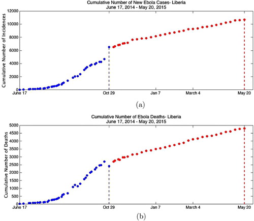
Figure 2. Fitting results. (a) Piecewise fit of cumulative incidences. The WHO reported cumulative incidences are plotted together with the model ${\tilde{M}}_5$ output. The model ${\tilde{M}}_5$ is evaluated with the fitted parameters given in Table 5. (b) Piecewise fit of cumulative deaths. The WHO reported cumulative deaths are plotted together with the model ${\tilde{M}}_5$ output. The model ${\tilde{M}}_5$ is evaluated with the fitted parameters given in Table 5.

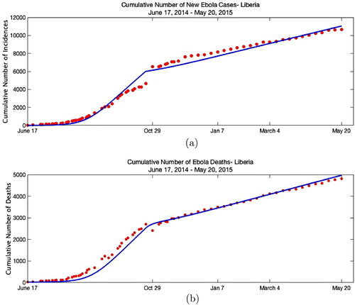
Table 3. List of nested models.

Model	Brief summary
$M_1$	No exposed class, no isolated class, no social distancing
$M_2$	With exposed class, no isolated class, no social distancing
$M_3$	No exposed class, with isolated class, no social distancing
$M_4$	With exposed class, with isolated class, no social distancing
$M_5$	No exposed class, no isolated class, with social distancing
$M_6$	With exposed class, no isolated class, with social distancing
$M_7$	No exposed class, with isolated class, with social distancing
$M_8$	With exposed class, with isolated class, with social distancing

As for every iterative optimization procedure, it is crucial to define initial values for each parameter that would find a global minimum. In an attempt to choose the best initial parameter values for the iterative solver, we performed the following procedure. Because of the structural identifiability issues of the models considered in this research, the rate that the recovered individuals loose their infectiousness is fixed, that is η is set to 1/25 (details are given in Section 3). The incubation period of the Ebola is 2 to 21 days, hence the initial guess for the parameter σ is set to 1/12. A random number generator is used to generate initial values for α, ${\alpha }_2$, γ and ${\gamma }_2$ on the interval [0.05, 2], initial values for $q_1$ and $q_2$ on the interval [0,1], initial value of ν on the interval [0.1, 2]. The proportion of isolated in all infected classes is targeted for $70\mathrm{\%}$. Thus, with the assumption that $\xi /\left(\xi +\alpha +\gamma \right)\approx 0.7$, the value for ξ was then calculated as $\frac{7}{3}(\alpha +\gamma )$. The basic reproduction number ${\mathcal{R}}_0$ of the models $M_1$, $M_2$, $M_5$ and $M_6$ is given by ${\mathcal{R}}_0=\frac{\beta S\left(0\right)}{\alpha +\gamma }+\frac{\gamma q_1\beta S\left(0\right)}{\eta (\alpha +\gamma )}+\frac{\alpha q_2\beta S\left(0\right)}{\nu (\alpha +\gamma )}.$ The basic reproduction number ${\mathcal{R}}_0$ of the models $M_3$ and $M_7$ is given by ${\mathcal{R}}_0=\frac{\beta S\left(0\right)}{\alpha +\gamma +\xi }+\frac{\gamma q_1\beta S\left(0\right)}{\eta (\alpha +\gamma +\xi )}+\frac{\alpha q_2\beta S\left(0\right)}{\nu (\alpha +\gamma +\xi )}+\frac{\xi {\gamma }_2{q}_1\beta S\left(0\right)}{\eta ({\alpha }_2+{\gamma }_2)(\alpha +\gamma +\xi ))}.$ The basic reproduction number ${\mathcal{R}}_0$ of the models $M_4$ and $M_8$ is given by ${\mathcal{R}}_0=\frac{\beta S\left(0\right)}{\alpha +\gamma +\xi }+\frac{q_1\beta S\left(0\right)({\alpha }_2\gamma +\gamma {\gamma }_2+\xi {\gamma }_2)}{\eta ({\alpha }_2+{\gamma }_2)(\alpha +\gamma +\xi )}+\frac{\alpha q_2\beta S\left(0\right)}{\nu (\alpha +\gamma +\xi )}.$ A random value for ${\mathcal{R}}_0$ on the interval (http://www.livescience.com/48962-ebola-transmission-rate-down.html) [1, 3] is selected, then using the value of ${\mathcal{R}}_0$ the initial guess for the parameter β is obtained.

The results of the fitting with SSE values of each model are presented in Table 4. Since, for each model different number of parameters are fitted comparing SSE values in determining the best model is not appropriate. Hence, the corrected Akaike Information Criterion (AIC) is used to decide which model(s) best describes the data [2].

Table 4. List of SSE and AIC for different models.

Model	SSE	${\mathcal{R}}_0$	Param fitted	AIC${}_c$	${\mathrm{\Delta }}_j$	Relative likelihood
1	$2.20303\times {10}^7$	$1.00113$	6	899.5	106.0	$9.71\times {10}^{-24}$
2	$5.34211\times {10}^7$	$1.00122$	7	964.0	170.5	$9.68\times {10}^{-38}$
3	$1.01435\times {10}^8$	$0.99719$	9	1014.1	220.5	$1.29\times {10}^{-48}$
4	$4.63683\times {10}^8$	$1.11368$	10	1123.2	329.6	$2.62\times {10}^{-72}$
5	$4.67945\times {10}^6$	$1.00107$	7	793.5	−	$0.998$
6	$6.77800\times {10}^6$	$1.75238$	8	822.0	28.5	$6.50\times {10}^{-7}$
7	$6.66748\times {10}^6$	$29.8094$	10	826.2	32.7	$7.89\times {10}^{-8}$
8	$4.73790\times {10}^6$	$537.240$	11	805.1	11.6	$0.002$

${\mathrm{AIC}}_c=n\ln \left(\frac{\mathrm{SSE}}{n}\right)+2K+\frac{2K(K+1)}{n-K-1},$where n is the number of data points and K is the number of parameters fitted plus one.The computed AIC${}_c$ values for all models are listed in Table 4. The smaller the AIC${}_c$ for a model, the better that model describes the data. As seen in Table 4, $M_5$ isthe model with the smallest AIC${}_c$, with AIC${}_{\mathrm{cmin}}=796.1.$ Comparing all the other models to the bestmodel ($M_5$), we compute ${\mathrm{\Delta }}_j$ as ${\mathrm{\Delta }}_j={\mathrm{AIC}}_{c_j}-{\mathrm{AIC}}_{\mathrm{cmin}}.$The last column in the Table 4 lists the relative likelihood of the model j, given by $w_j=\frac{{\mathrm{e}}^{-{\mathrm{\Delta }}_j/2}}{\sum _{i=1}^8{\mathrm{e}}^{-{\mathrm{\Delta }}_i/2}}.$Since, the models are nested, some models might still have support in the data whileothers can be completely ruled out. The models whose relative likelihood sum up to $\sum w_j>0.95$ give the models that explain the data. The relative likelihood of $M_5$ is 0.99, greater thanthe threshold value 0.95, which means that the model $M_5$ solely explains the data.According to these results, we see that the simplest model (model with no exposed orisolated classes) which incorporates the social distancing is the model that bestdescribes the Ebola outbreak data in Liberia. That is the human behaviour had a significant impact on the transmission of the Ebola outbreak inLiberia.

Data for several of the recently affected countries by Ebola, such as Sierra Leone, Liberia and Guinea can be obtained from [28]. The cumulative number of incidences and deaths in Liberia were reported by WHO starting on 17 June 2014 continuing till 20May 2015. The outbreak in Liberia was declared over on 9 May 2015, 42 days after the death of the last confirmed case. We collected the data from these reports published by WHO at its website [28]. The cumulative cases are the total number of confirmed, probable and suspected cases. The data are not evenly distributed till 26 November 2015. After that the reports are given every week, and hence the data after 26th November are evenly distributed. Observing the data, one can see that there is an unusual increase of cumulative cases on 29th October and a decrease on cumulative deaths. The WHO report on 29th October states that ‘increase in the cumulative total number of cases compared with the situation report of 22nd October results from a more comprehensive assessment of patient databases. The additional $3792$ cases have occurred throughout the epidemic period, not only since 22nd October [27] '. (All the WHO reports are available from the authors if requested.)

As seen from Figure 1(a), there is a jump in the cumulative number of incidences reported by WHO on 29 October 2014. To incorporate the steep revision made on 29th October through the epidemic period, time-dependent social distancing rate is imposed, hence model $M_5$ becomes (7) ${\tilde{M}}_5:\left\{\begin{array}{ll}\frac{\mathrm{d}S}{\mathrm{d}t}& =-\beta S(I+q_{1}R+q_{2}D){\mathrm{e}}^{-(\kappa +H(t-t^{\ast }\left){\kappa }_1\right)\left((I+R+D)/(S+I+R+D)\right)},\\ \frac{\mathrm{d}I}{\mathrm{d}t}& =\beta S(I+q_{1}R+q_{2}D){\mathrm{e}}^{-(\kappa +H(t-t^{\ast }\left){\kappa }_1\right)\left((I+R+D)/(S+I+R+D)\right)}-(\gamma +\alpha )I,\\ \frac{\mathrm{d}R}{\mathrm{d}t}& =\gamma I-\eta R,\\ \frac{\mathrm{d}D}{\mathrm{d}t}& =\alpha I-\nu D,\\ \frac{\mathrm{d}{R}_m}{\mathrm{d}t}& =\eta R+\nu D.\end{array}\right.$(7) Here $H\left(t\right)$ denotes the Heaviside function and $t^{\ast }$ is the time data point corresponding to 29 October 2014. The fitted values of the parameters of the model ${\tilde{M}}_5$ are given in Table 5. As given in Table 5, the estimated period of infectiousness $1/(\alpha +\gamma )$ agrees with the results given in [12]. The confidence intervals presented in Table 5 are computed using the Statistical Toolbox (nlparci) in MATLAB. For the death data, we use data reported by WHO. However, for a fraction of hospitalized cases the definitive outcome (death or recovery) was not recorded in individual records. Therefore, the cumulative number of deaths reported to the WHO during the Ebola outbreak in West Africa was an underestimate of the actual number. In particular, work of the WHO-led team [26] suggests that early in the epidemic the case-fatality proportion might have been up to 70% while the published WHO data for Liberia for the early stage of the epidemic suggest that it was approximately 50%. To examine the impact of this discrepancy on the estimated parameters of the selected model, we increase the death cases by 20% and fit to the increased data. The new estimates of the parameters are presented in Table 6 together with the confidence intervals. Results suggest that the change in the parameters is relatively small.

Table 5. Parameter estimates of the Ebola model ${\tilde{M}}_5$.

Parameter	Estimate	Confidence intervals
β	$4.9661\times {10}^{(-8)}$	$[0.2816\times {10}^{(-8)},9.6506\times {10}^{(-8)}]$
$q_1$	0.262923557067464	$[-1.09,1.61]$
$q_2$	0.030495560371388	$[-8.05,8.11]$
α	0.081817517646725	$[0.08180,.0.08183]$
γ	0.098540816938738	$[0.0928,0.1043]$
ν	0.641566115689430	$[0.4549,0.8282]$
κ	$1.803173872675241\times {10}^{\left(3\right)}$	$[-1.1983\times {10}^{\left(3\right)},4.8046\times {10}^{\left(3\right)}]$
${\kappa }_1$	$4.575388752640867\times {10}^{\left(3\right)}$	$[-5.5067\times {10}^{\left(3\right)},14.6575\times {10}^{\left(3\right)}]$

Table 6. Parameter estimates of the Ebola model ${\tilde{M}}_5$ when cumulative deaths have been increased by 20$\mathrm{\%}$.

Parameter	Estimate	Confidence intervals
β	$4.6514\times {10}^{(-8)}$	$[-2.1278\times {10}^{(-8)},11.4306\times {10}^{(-8)}]$
$q_1$	0.219017159832389	$[-0.6476,1.0856]$
$q_2$	1.200962559288544	$[-10.7588,13.1607]$
α	0.098162837678339	$[0.0084,0.1879]$
γ	0.088544427646715	$[0.0034,0.1737]$
ν	0.806684770321498	$[0.6967,0.9167]$
κ	$1.688908621622106\times {10}^{\left(3\right)}$	$[-0.2427\times {10}^{\left(3\right)},3.6205\times {10}^{\left(3\right)}]$
${\kappa }_1$	$4.303164470658873\times {10}^{\left(3\right)}$	$[-2.4424\times {10}^{\left(3\right)},11.0488\times {10}^{\left(3\right)}]$

3. Identifiability and parameter estimation

The purpose of this study is to evaluate the efficacy of control measures implemented to limit the spread of the Ebola outbreak. Hence, these results highly depend on accurately estimating the parameters of the outbreak model from the reported data by the health organizations. So, it is crucial to study the well-posedness of the parameter estimation problem for the given observations such as cumulative incidences and deaths. A model is said to be identifiable if for given large enough set of data points, free of errors, it is theoretically possible to uniquely determine the parameter values from the observations that generated these data points. If two or more parameter sets can lead to the same observational output, the model is called non-identifiable. If the model is not identifiable, then it is not possible to estimate the ‘true values’ of the parameters. There are multiple ways to test for the identifiability of a model: Taylor's or Generating series approaches, identifiability tableaus, differential algebra approach and others [6]. In this study, we use the differential algebra approach which is designed specifically to test for the identifiability of (nonlinear) differential equation models. We briefly explain the differential algebra approach here, but for more detailed review we refer the reader to [17]. To set up the problem, without loss of generality the outbreak models can be expressed in the following compact form: (8) ${\mathit{x}}^{\prime }=f\left(\mathit{x}\right(t),\mathit{p})\mathit{x}\left(0\right)={\mathit{x}}_0,$(8) where $\mathit{p}$ denotes the parameters of the system, $\mathit{x}\left(t\right)$ denotes the states of the system and ${\mathit{x}}_0$ is the initial values. The observations, which in this study are cumulative number of cases and deaths, are given by the output function $g\left(\mathit{x}\right(t),\mathit{p})$. The definition of the structural identifiability is given in the literature as [17].

Definition 3.1

A parameter set $\mathit{p}$ is called structurally globally (or uniquely) identifiable if for every $\mathit{q}$ in the parameter space $g\left(\mathit{x}\right(t),\mathit{p})=g\left(\mathit{x}\right(t),\mathit{q})⟹\mathit{p}=\mathit{q}.$

That is any unequal parameter set yields different observations and hence the corresponding noise-free data are as well distinct.

The first step in differential algebra approach is to find the input–output equations of the dynamical model (8(8) ${\mathit{x}}^{\prime }=f\left(\mathit{x}\right(t),\mathit{p})\mathit{x}\left(0\right)={\mathit{x}}_0,$(8) ). This is done by reducing the model to its characteristic set via Ritt's algorithm. The characteristic set is then used to derive the input–output equations which contains all the identifiability information of the model. Input–output equations simply put are a subset of the characteristic set. The characteristic set of a dynamical ODE model is not unique, hence it depends on the chosen ranking of the state variables. However, the coefficients of the input–output equation can be fixed uniquely by normalizing the equations to make them monic.

To illustrate the approach on a simple example, consider the following simplification of the model $M_1$, (9) $\begin{array}{rl}& S^{\prime }=-\beta SI,\\ & I^{\prime }=\beta SI-(\alpha +\gamma )I,\\ & R^{\prime }=\gamma I.\end{array}$(9) Suppose now that we observe the cumulative incidences. Hence, $g_1\left(\mathit{x}\right(t),\mathit{p})=C\left(t\right)={\int }_0^t\beta S\left(\tau \right)I\left(\tau \right)\mathrm{d}\tau =S_0-S\left(t\right).$ If we know the initial number of susceptibles, $S_0$, cumulative incidences are equivalent to observing S. To obtain an input–output equation, we eliminate the unobserved states, I and R from the system, and obtain equation in S and its derivatives. We express I from the first equation, we differentiate I with respect to t and we eliminate I and $I^{\prime }$ from the second equation. We obtain the following input–output equation: (10) $-S^{″}S+(S^{\prime }{)}^2+\beta S^{\prime }{S}^2-(\alpha +\gamma )S^{\prime }S=0.$(10) Within the differential algebra approach, the ODE model is said to be structurally identifiable if the map from the parameter space to the coefficients of the input–output equations is injective [10]. Thus the definition of the structural identifiability becomes

Definition 3.2

The dynamical model is globally identifiable if and only if $c\left(\mathit{p}\right)=c\left(\mathit{q}\right)⟹\mathit{p}=\mathit{q},$ where $c\left(\mathit{p}\right)$ are the coefficients of the normalized input–output equation.

Suppose to the contrary that there exist another set of parameters $\mathit{q}=[{\beta }_q,{\alpha }_q,{\gamma }_q]$ which produced the same observation, then $c\left(\mathit{p}\right)=c\left(\mathit{q}\right)$ yield to the following set of equations: $\beta ={\beta }_q,\alpha +\gamma ={\alpha }_q+{\gamma }_q.$ Therefore, if we only observe cumulative incidence, we can only identify β and the sum of $\alpha +\gamma$ but not α and γ individually. So, we claim that the model (9(9) $\begin{array}{rl}& S^{\prime }=-\beta SI,\\ & I^{\prime }=\beta SI-(\alpha +\gamma )I,\\ & R^{\prime }=\gamma I.\end{array}$(9) ) is not identifiable from the cumulative incidence observations.

Suppose now that in addition to the cumulative incidence, we observe cumulative deaths, which for most diseases, including Ebola, are done. In this case, we add another variable CD$\left(t\right)$ which gives the cumulative deaths. We have CD${}^{\prime }\left(t\right)=\alpha I$ and the output function is $g_2\left(\mathit{x}\right(t),\mathit{p})=\mathrm{CD}\left(t\right)=\mathrm{CD}\left(0\right)+{\int }_0^t\alpha I\left(\sigma \right)\mathrm{d}\sigma .$ In this case, in addition to the input–output equation (10(10) $-S^{″}S+(S^{\prime }{)}^2+\beta S^{\prime }{S}^2-(\alpha +\gamma )S^{\prime }S=0.$(10) ), we obtain a second input–output equation which may contain CD and its derivatives. To obtain the second input–output equation, in the equation CD${}^{\prime }=\alpha I$ we replace I with its expression in terms of S and $S^{\prime }$ obtained from the first equation. We get $\beta S{\mathrm{CD}}^{″}+\alpha S^{\prime }=0.$ So, if there is another input–output equation with parameters ${\beta }_q$ and ${\alpha }_q$, then $\beta ={\beta }_q$ and $\alpha ={\alpha }_q$. Thus we can identify β, α and $\alpha +\gamma$. But since we can identify α and $\alpha +\gamma$, this means that we can identify γ. Therefore, model (9(9) $\begin{array}{rl}& S^{\prime }=-\beta SI,\\ & I^{\prime }=\beta SI-(\alpha +\gamma )I,\\ & R^{\prime }=\gamma I.\end{array}$(9) ) is identifiable only when both cumulative incidences and deaths are observed.

The situation is similar with the model $M_1$ (1(1) $\mathrm{Model}1\left(M_1\right):\left\{\begin{array}{l}\frac{\mathrm{d}S}{\mathrm{d}t}=-\beta S(I+q_{1}R+q_{2}D),\\ \frac{\mathrm{d}I}{\mathrm{d}t}=\beta S(I+q_{1}R+q_{2}D)-(\gamma +\alpha )I,\\ \frac{\mathrm{d}R}{\mathrm{d}t}=\gamma I-\eta R,\\ \frac{\mathrm{d}D}{\mathrm{d}t}=\alpha I-\nu D,\\ \frac{\mathrm{d}{R}_m}{\mathrm{d}t}=\eta R+\nu D,\end{array}\right.$(1) ). We need to fit both cumulative incidences and cumulative deaths to expect identifiability. With the model $M_1$ computing the input–output equation is not possible by hand. We use MAPLE to derive the input–output equation in each case. After that, we use MATHEMATICA to solve the systems $c\left(\mathit{p}\right)=c\left(\mathit{q}\right)$ for the coefficients. In the case of the model $M_1$ (1(1) $\mathrm{Model}1\left(M_1\right):\left\{\begin{array}{l}\frac{\mathrm{d}S}{\mathrm{d}t}=-\beta S(I+q_{1}R+q_{2}D),\\ \frac{\mathrm{d}I}{\mathrm{d}t}=\beta S(I+q_{1}R+q_{2}D)-(\gamma +\alpha )I,\\ \frac{\mathrm{d}R}{\mathrm{d}t}=\gamma I-\eta R,\\ \frac{\mathrm{d}D}{\mathrm{d}t}=\alpha I-\nu D,\\ \frac{\mathrm{d}{R}_m}{\mathrm{d}t}=\eta R+\nu D,\end{array}\right.$(1) ), we obtain the following solutions: (11) $\begin{array}{rl}\beta & ={\beta }_q,q_1=q_{1q},q_2=q_{2q},\gamma ={\gamma }_q,\alpha ={\alpha }_q,\eta ={\eta }_q,\nu ={\nu }_q\\ \beta & ={\beta }_q,\frac{\gamma q_1}{\alpha }=q_{2q},\frac{\alpha q_2}{\gamma }=q_{1q},\gamma ={\gamma }_q,\alpha ={\alpha }_q,\eta ={\nu }_q,\nu ={\eta }_q.\end{array}$(11) Hence, there are two sets of solutions and therefore, the model $M_1$ (1(1) $\mathrm{Model}1\left(M_1\right):\left\{\begin{array}{l}\frac{\mathrm{d}S}{\mathrm{d}t}=-\beta S(I+q_{1}R+q_{2}D),\\ \frac{\mathrm{d}I}{\mathrm{d}t}=\beta S(I+q_{1}R+q_{2}D)-(\gamma +\alpha )I,\\ \frac{\mathrm{d}R}{\mathrm{d}t}=\gamma I-\eta R,\\ \frac{\mathrm{d}D}{\mathrm{d}t}=\alpha I-\nu D,\\ \frac{\mathrm{d}{R}_m}{\mathrm{d}t}=\eta R+\nu D,\end{array}\right.$(1) ) is not identifiable. We select and fix η from additional biological information. Because η is the duration of infectiousness of the recovered class and it is estimated to last up to 7 weeks [29], we set $\eta =1/25$. That is having $\eta ={\eta }_q=1/25$ in (11(11) $\begin{array}{rl}\beta & ={\beta }_q,q_1=q_{1q},q_2=q_{2q},\gamma ={\gamma }_q,\alpha ={\alpha }_q,\eta ={\eta }_q,\nu ={\nu }_q\\ \beta & ={\beta }_q,\frac{\gamma q_1}{\alpha }=q_{2q},\frac{\alpha q_2}{\gamma }=q_{1q},\gamma ={\gamma }_q,\alpha ={\alpha }_q,\eta ={\nu }_q,\nu ={\eta }_q.\end{array}$(11) ), the parameters of the model $M_1$ (1(1) $\mathrm{Model}1\left(M_1\right):\left\{\begin{array}{l}\frac{\mathrm{d}S}{\mathrm{d}t}=-\beta S(I+q_{1}R+q_{2}D),\\ \frac{\mathrm{d}I}{\mathrm{d}t}=\beta S(I+q_{1}R+q_{2}D)-(\gamma +\alpha )I,\\ \frac{\mathrm{d}R}{\mathrm{d}t}=\gamma I-\eta R,\\ \frac{\mathrm{d}D}{\mathrm{d}t}=\alpha I-\nu D,\\ \frac{\mathrm{d}{R}_m}{\mathrm{d}t}=\eta R+\nu D,\end{array}\right.$(1) ) become identifiable. Since, the model $M_1$ (1(1) $\mathrm{Model}1\left(M_1\right):\left\{\begin{array}{l}\frac{\mathrm{d}S}{\mathrm{d}t}=-\beta S(I+q_{1}R+q_{2}D),\\ \frac{\mathrm{d}I}{\mathrm{d}t}=\beta S(I+q_{1}R+q_{2}D)-(\gamma +\alpha )I,\\ \frac{\mathrm{d}R}{\mathrm{d}t}=\gamma I-\eta R,\\ \frac{\mathrm{d}D}{\mathrm{d}t}=\alpha I-\nu D,\\ \frac{\mathrm{d}{R}_m}{\mathrm{d}t}=\eta R+\nu D,\end{array}\right.$(1) ) is the simplest model among the nested models of $M_1$ through $M_8$, we fix η to 1/25 while estimating the parameters of models $M_1$ through $M_8$.

Structural identifiability analysis of the model ${\tilde{M}}_5$ (7(7) ${\tilde{M}}_5:\left\{\begin{array}{ll}\frac{\mathrm{d}S}{\mathrm{d}t}& =-\beta S(I+q_{1}R+q_{2}D){\mathrm{e}}^{-(\kappa +H(t-t^{\ast }\left){\kappa }_1\right)\left((I+R+D)/(S+I+R+D)\right)},\\ \frac{\mathrm{d}I}{\mathrm{d}t}& =\beta S(I+q_{1}R+q_{2}D){\mathrm{e}}^{-(\kappa +H(t-t^{\ast }\left){\kappa }_1\right)\left((I+R+D)/(S+I+R+D)\right)}-(\gamma +\alpha )I,\\ \frac{\mathrm{d}R}{\mathrm{d}t}& =\gamma I-\eta R,\\ \frac{\mathrm{d}D}{\mathrm{d}t}& =\alpha I-\nu D,\\ \frac{\mathrm{d}{R}_m}{\mathrm{d}t}& =\eta R+\nu D.\end{array}\right.$(7) ) is not possible by means of differential algebra approach, since the approach requires $\mathit{f}\left(\mathit{x}\right(t),\mathit{p})$ to be rational functions of the state variables $\mathit{x}\left(t\right)$. Because of the social distancing term, we cannot further analyse the structural identifiability of the model${\tilde{M}}_5$, but we study the practical identifiability of the model ${\tilde{M}}_5$ (7(7) ${\tilde{M}}_5:\left\{\begin{array}{ll}\frac{\mathrm{d}S}{\mathrm{d}t}& =-\beta S(I+q_{1}R+q_{2}D){\mathrm{e}}^{-(\kappa +H(t-t^{\ast }\left){\kappa }_1\right)\left((I+R+D)/(S+I+R+D)\right)},\\ \frac{\mathrm{d}I}{\mathrm{d}t}& =\beta S(I+q_{1}R+q_{2}D){\mathrm{e}}^{-(\kappa +H(t-t^{\ast }\left){\kappa }_1\right)\left((I+R+D)/(S+I+R+D)\right)}-(\gamma +\alpha )I,\\ \frac{\mathrm{d}R}{\mathrm{d}t}& =\gamma I-\eta R,\\ \frac{\mathrm{d}D}{\mathrm{d}t}& =\alpha I-\nu D,\\ \frac{\mathrm{d}{R}_m}{\mathrm{d}t}& =\eta R+\nu D.\end{array}\right.$(7) ) by Monte Carlo simulations.

Let $\mathit{p}=[\beta ,q_1,q_2,\alpha ,\gamma ,\eta ,\nu ,\kappa ,{\kappa }_1]$ denote the parameters, and $\mathit{x}\left(t\right)=\left[S\right(t),I(t),R(t),D(t),R_m(t\left)\right]$ denote the states of the system (7(7) ${\tilde{M}}_5:\left\{\begin{array}{ll}\frac{\mathrm{d}S}{\mathrm{d}t}& =-\beta S(I+q_{1}R+q_{2}D){\mathrm{e}}^{-(\kappa +H(t-t^{\ast }\left){\kappa }_1\right)\left((I+R+D)/(S+I+R+D)\right)},\\ \frac{\mathrm{d}I}{\mathrm{d}t}& =\beta S(I+q_{1}R+q_{2}D){\mathrm{e}}^{-(\kappa +H(t-t^{\ast }\left){\kappa }_1\right)\left((I+R+D)/(S+I+R+D)\right)}-(\gamma +\alpha )I,\\ \frac{\mathrm{d}R}{\mathrm{d}t}& =\gamma I-\eta R,\\ \frac{\mathrm{d}D}{\mathrm{d}t}& =\alpha I-\nu D,\\ \frac{\mathrm{d}{R}_m}{\mathrm{d}t}& =\eta R+\nu D.\end{array}\right.$(7) ). We assume that initial values of the system can be determined by other means, and we are only interested in the parameters that would determine the reproduction number. Since for identifiability issues, we fix $\eta =1/25$, through least squares, we would like to recover the true parameter set, ${\mathit{p}}_0=[\beta ,q_1,q_2,\alpha ,\gamma ,\nu ,\kappa ,{\kappa }_1].$ The observations of the system, ${\mathit{y}}_1,{\mathit{y}}_2,\dots ,{\mathit{y}}_n$ made at the data time points $t_1,t_2,\dots t_n$, are obtained by adding the observational errors to the model output, hence ${\mathit{y}}_i=\mathit{g}\left(\mathit{x}\right(t_i),{\mathit{p}}_0)+{\mathit{ϵ}}_i,$ where $\mathit{g}\left(\mathit{x}\right(t),\mathit{p})=\left(g_1\right(\mathit{x}\left(t\right),{\mathit{p}}_0),g_2(\mathit{x}\left(t\right),{\mathit{p}}_0\left)\right)$ represents the vector output of the system involving both cumulative incidences and deaths and ${\mathit{y}}_i=(y_i^1,y_i^2)$ is the vector of observations made at discrete time $t_k,k=1,2,\dots ,n$. The random variables ${\mathit{ϵ}}_i$ represent the measurement errors which cause the observations $\mathit{g}\left(\mathit{x}\right(t_i),{\mathit{p}}_0)$ to drift away from the smooth exact path $\mathit{g}\left(\mathit{x}\right(t),{\mathit{p}}_0)$. In a more general setting, the errors satisfy the following form, which allows fairly wide range of error models, (12) ${\mathit{ϵ}}_i=\mathit{g}\left(\mathit{x}\right(t_i),{\mathit{p}}_0{)}^f{\epsilon }_i,$(12) where $f\ge 0$. ${\epsilon }_i$ are assumed to be independent, identically distributed random variables with mean zero and finite variance ${\sigma }_0^2$. The mean and the variance of the random variables ${\mathit{y}}_i$ satisfy, $\mathbb{E}\left({\mathit{y}}_i\right)=\mathit{g}\left(\mathit{x}\right(t_i),{\mathit{p}}_0)$, Var$\left({\mathit{y}}_i\right)=\mathit{g}\left(\mathit{x}\right(t_i),{\mathit{p}}_0{)}^{2f}{\sigma }_0^2,$ respectively. For the model (7(7) ${\tilde{M}}_5:\left\{\begin{array}{ll}\frac{\mathrm{d}S}{\mathrm{d}t}& =-\beta S(I+q_{1}R+q_{2}D){\mathrm{e}}^{-(\kappa +H(t-t^{\ast }\left){\kappa }_1\right)\left((I+R+D)/(S+I+R+D)\right)},\\ \frac{\mathrm{d}I}{\mathrm{d}t}& =\beta S(I+q_{1}R+q_{2}D){\mathrm{e}}^{-(\kappa +H(t-t^{\ast }\left){\kappa }_1\right)\left((I+R+D)/(S+I+R+D)\right)}-(\gamma +\alpha )I,\\ \frac{\mathrm{d}R}{\mathrm{d}t}& =\gamma I-\eta R,\\ \frac{\mathrm{d}D}{\mathrm{d}t}& =\alpha I-\nu D,\\ \frac{\mathrm{d}{R}_m}{\mathrm{d}t}& =\eta R+\nu D.\end{array}\right.$(7) ), the cumulative number of incidences can be determined from the susceptible population by the following representation: ${\int }_0^t\beta S(I+q_{1}R+q_{2}D){\mathrm{e}}^{-(\kappa +H(t-t^{\ast }\left){\kappa }_1\right)\left((I+R+D)/(S+I+R+D)\right)}=S\left(0\right)-S\left(t\right),$ and the cumulative deaths, CD$\left(t\right),$ will be evaluated by augmenting the following differential equation to the model (7(7) ${\tilde{M}}_5:\left\{\begin{array}{ll}\frac{\mathrm{d}S}{\mathrm{d}t}& =-\beta S(I+q_{1}R+q_{2}D){\mathrm{e}}^{-(\kappa +H(t-t^{\ast }\left){\kappa }_1\right)\left((I+R+D)/(S+I+R+D)\right)},\\ \frac{\mathrm{d}I}{\mathrm{d}t}& =\beta S(I+q_{1}R+q_{2}D){\mathrm{e}}^{-(\kappa +H(t-t^{\ast }\left){\kappa }_1\right)\left((I+R+D)/(S+I+R+D)\right)}-(\gamma +\alpha )I,\\ \frac{\mathrm{d}R}{\mathrm{d}t}& =\gamma I-\eta R,\\ \frac{\mathrm{d}D}{\mathrm{d}t}& =\alpha I-\nu D,\\ \frac{\mathrm{d}{R}_m}{\mathrm{d}t}& =\eta R+\nu D.\end{array}\right.$(7) ), $\frac{\mathrm{d}CD}{\mathrm{d}t}=\alpha I.$ Hence, $g_1\left(\mathit{x}\right(t),\mathit{p})=S\left(0\right)-S(t,\mathit{p})$ and $g_2\left(\mathit{x}\right(t),\mathit{p})=\mathrm{CD}(t,\mathit{p}).$ With this setting, the least squares problem is to find the parameter set $\hat{\mathit{p}}$ which minimizes the following cost functional: (13) $\hat{\mathit{p}}=\underset{\mathit{p}}{min}J\left(\mathit{p}\right)=\underset{\mathit{p}}{min}\sum _{i=1}^n\left((y_i^1-g_1(\mathit{x}\left(t_i\right),\mathit{p}{)}^2+(y_i^2-g_2(\mathit{x}\left(t_i\right),\mathit{p}{)}^2\right).$(13)

The Monte Carlo simulations we performed are outlined in the following steps. We take the estimated parameters given in Table 5 as the true parameter set${\mathit{p}}_0$.

1. Solve the epidemiological model numerically with the true parameters ${\mathit{p}}_0$ and obtain the output vector $\mathit{g}\left(\mathit{x}\right(t),{\mathit{p}}_0)$ at the discrete data time points $\{t_k{\}}_{k=1}^n.$

2. Generate M=1000 residual vectors ${\hat{\mathit{r}}}_i$ drawn from a normal distribution whose mean is the output vector computed in step (1) and standard deviation is the ${\sigma }_0\mathrm{\%}$ of the mean.

3. Fit the model ${\tilde{M}}_5$ to each of the M simulated data sets by minimizing the cost functional (13(13) $\hat{\mathit{p}}=\underset{\mathit{p}}{min}J\left(\mathit{p}\right)=\underset{\mathit{p}}{min}\sum _{i=1}^n\left((y_i^1-g_1(\mathit{x}\left(t_i\right),\mathit{p}{)}^2+(y_i^2-g_2(\mathit{x}\left(t_i\right),\mathit{p}{)}^2\right).$(13) ) using the Nelder–Mead algorithm implemented in MATALB to estimate the parameter set ${\hat{\mathit{p}}}_j$ for $j=1,2,\dots ,M$.

4. Calculate the average relative estimation error for each parameter in the set $\mathit{p}$ by $\mathrm{ARE}\left(p^{\left(k\right)}\right)=100\mathrm{\%}\frac{1}{M}\sum _{j=1}^M\frac{|p_0^{\left(k\right)}-p_j^{\left(k\right)}|}{p_0^{\left(k\right)}},$ where $p^{\left(k\right)}$ is the kth parameter in the set $\mathit{p}$, $p_0^{\left(k\right)}$ is the kth parameter in the set ${\mathit{p}}_0$ and $p_j^{\left(k\right)}$ is the kth parameter in the set ${\mathit{p}}_j$.

5. Repeat steps 1 through 4 with increasing level of noise, that is take ${\sigma }_0=0,5,20\mathrm{\%}.$

We present the results of Monte Carlo simulations in Tables 7 and 8 with AREs computed with increasing error levels ${\sigma }_0=0,5,20\mathrm{\%}$. The computed AREs give an insight about the identifiability of the parameters of the model ${\tilde{M}}_5$. If a model is structurally identifiable, then when there is no noise in the data (when ${\sigma }_0=0$), the AREs would be 0 or very close to 0. As the standard deviation (${\sigma }_0$) increases, the AREs of the parameters increase as well. The parameters which are not practically identifiable would be very sensitive to the error levels in the data and AREs of those parameters would be larger than the measurement error (for example, see $q_1$ and $q_2$ in Table 7). Since $q_1$ and $q_2$ are practically unidentifiable, we fix those parameters to the estimated values, and observe that the AREs of the rest of the parameters have increased with the exception of unidentifiable parameters κ and ${\kappa }_1$ (see Table 8).

Table 7. Monte Carlo simulations.

Parameter	ARE 0%	ARE 5%	ARE 20%
β	0.0%	3.65%	8.05%
$q_1$	0.0%	18.70%	31.37%
$q_2$	0.0%	163.34%	212.64%
α	0.0%	6.72%	15.27%
γ	0.0%	7.32%	17.11%
ν	0.0%	4.22%	7.94%
κ	0.0%	5.27%	13.49%
${\kappa }_1$	0.0%	9.03%	22.51%

Table 8. Monte Carlo simulations when $q_1$ and $q_2$ are fixed to estimated values.

Parameter	ARE 0%	ARE 5%	ARE 20%
β	0.0%	1.12%	3.97%
α	0.0%	2.36%	8.70%
γ	0.0%	1.56%	5.91%
ν	0.0%	4.97%	10.95%
κ	0.0%	6.87%	30.10%
${\kappa }_1$	0.0%	4.35%	19.22%

4. Control strategies

Main control strategies for Ebola include early identification and isolation of cases, contact tracing and quarantining of suspected contacts, proper personal protection, safely conducted burials, improved education and social awareness about risk factors of Ebola infection and individual protective measures. Quarantine and isolation have been previously modelled in connection with SARS [19]. The impact of social awareness has been included in several articles on Ebola [11,21]. The contact tracing is implicitly incorporated in the quarantine and isolation but Ebola model with explicit contact tracing was considered in [1]. We include quarantine, isolation, education (awareness), safe burial and social distancing. The WHO publishes ‘How to conduct safe and dignified burial of a patient who has died from suspected or confirmed Ebola virus disease’ on October 2014 (http://www.who.int/csr/resources/publications/ebola/safe-burial-protocol/en/).

To elucidate the impact of control measures on the parameters of our baseline model (${\tilde{M}}_5$), we consider an expanded model with the education included explicitly. We denote the non-educated susceptibles by $S_N$ and the educated susceptibles by $S_E$, quarantined susceptibles by $Q_S$, individuals in their incubation period by E, quarantined latent by $Q_E$ and isolated individuals by Q, recovered educated by $R_E$ and recovered non-educated by $R_N$. Quarantining occurs at a rate ${\rho }_E$ for educated individuals and rate ρ for others.

Quarantined susceptibles move to educated susceptible class at rate θ, infected individuals move to the isolation class at rate ξ and the quarantined latent individuals move to the isolation class at rate $k_2$. Isolated individuals recover at rate ${\gamma }_2$ and move to the educated recovered class. The state variables for the model with control measures are summarized in Table 9 and the parameters of the model are summarized in Table 10. The model with control measures takes the form: (14) $M_9:\left\{\begin{array}{l}\frac{\mathrm{d}{S}_N}{\mathrm{d}t}=-\rho S_N-{\beta }_N{S}_N(I+q_{E}E+q_{1E}{R}_E\\ +q_{1N}{R}_N+{\tilde{q}}_{2}D){\mathrm{e}}^{\left(-\tilde{\kappa }(I+E+R_N+R_E+D)\right)/(S+I+E+R_N+R_E+D)},\\ \frac{\mathrm{d}{S}_E}{\mathrm{d}t}=-{\rho }_E{S}_E+\theta Q_S-{\beta }_E{S}_E(I+q_{E}E+q_{1E}{R}_E+q_{1N}{R}_N\\ +{\tilde{q}}_{2}D){\mathrm{e}}^{\left(-\tilde{\kappa }(I+E+R_N+R_E+D)\right)/(S+I+E+R_N+R_E+D)},\\ \frac{\mathrm{d}{Q}_S}{\mathrm{d}t}=\rho S_N+{\rho }_E{S}_E-\theta Q_S,\\ \frac{\mathrm{d}E}{\mathrm{d}t}=({\beta }_N{S}_N+{\beta }_E{S}_E)(I+q_{E}E+q_{1E}{R}_E+q_{1N}{R}_N\\ +{\tilde{q}}_{2}D){\mathrm{e}}^{\left(-\tilde{\kappa }(I+E+R_N+R_E+D)\right)/(S+E+I+R_N+R_E+D)}-\rho E-\sigma E,\\ \frac{\mathrm{d}{Q}_E}{\mathrm{d}t}=\rho E-k_2{Q}_E,\\ \frac{\mathrm{d}I}{\mathrm{d}t}=\sigma E-(\gamma +\alpha +\xi )I,\\ \frac{\mathrm{d}Q}{\mathrm{d}t}=\xi I+k_2{Q}_E-({\alpha }_2+{\gamma }_2)Q,\\ \frac{\mathrm{d}{R}_E}{\mathrm{d}t}={\gamma }_{2}Q-\eta R_E,\\ \frac{\mathrm{d}{R}_N}{\mathrm{d}t}=\gamma I-\eta R_N,\\ \frac{\mathrm{d}D}{\mathrm{d}t}=\alpha I-\nu D,\\ \frac{\mathrm{d}{R}_m}{\mathrm{d}t}=\eta (R_E+R_N)+{\alpha }_{2}Q+\nu D,\end{array}\right.$(14) where $\tilde{\kappa }=\kappa +H(t-t^{\ast }){\kappa }_1$. To understand the impact of the control measures on the parameters, we collapse the model with control measures (14(14) $M_9:\left\{\begin{array}{l}\frac{\mathrm{d}{S}_N}{\mathrm{d}t}=-\rho S_N-{\beta }_N{S}_N(I+q_{E}E+q_{1E}{R}_E\\ +q_{1N}{R}_N+{\tilde{q}}_{2}D){\mathrm{e}}^{\left(-\tilde{\kappa }(I+E+R_N+R_E+D)\right)/(S+I+E+R_N+R_E+D)},\\ \frac{\mathrm{d}{S}_E}{\mathrm{d}t}=-{\rho }_E{S}_E+\theta Q_S-{\beta }_E{S}_E(I+q_{E}E+q_{1E}{R}_E+q_{1N}{R}_N\\ +{\tilde{q}}_{2}D){\mathrm{e}}^{\left(-\tilde{\kappa }(I+E+R_N+R_E+D)\right)/(S+I+E+R_N+R_E+D)},\\ \frac{\mathrm{d}{Q}_S}{\mathrm{d}t}=\rho S_N+{\rho }_E{S}_E-\theta Q_S,\\ \frac{\mathrm{d}E}{\mathrm{d}t}=({\beta }_N{S}_N+{\beta }_E{S}_E)(I+q_{E}E+q_{1E}{R}_E+q_{1N}{R}_N\\ +{\tilde{q}}_{2}D){\mathrm{e}}^{\left(-\tilde{\kappa }(I+E+R_N+R_E+D)\right)/(S+E+I+R_N+R_E+D)}-\rho E-\sigma E,\\ \frac{\mathrm{d}{Q}_E}{\mathrm{d}t}=\rho E-k_2{Q}_E,\\ \frac{\mathrm{d}I}{\mathrm{d}t}=\sigma E-(\gamma +\alpha +\xi )I,\\ \frac{\mathrm{d}Q}{\mathrm{d}t}=\xi I+k_2{Q}_E-({\alpha }_2+{\gamma }_2)Q,\\ \frac{\mathrm{d}{R}_E}{\mathrm{d}t}={\gamma }_{2}Q-\eta R_E,\\ \frac{\mathrm{d}{R}_N}{\mathrm{d}t}=\gamma I-\eta R_N,\\ \frac{\mathrm{d}D}{\mathrm{d}t}=\alpha I-\nu D,\\ \frac{\mathrm{d}{R}_m}{\mathrm{d}t}=\eta (R_E+R_N)+{\alpha }_{2}Q+\nu D,\end{array}\right.$(14) ) to the model ${\tilde{M}}_5$ as given in (7(7) ${\tilde{M}}_5:\left\{\begin{array}{ll}\frac{\mathrm{d}S}{\mathrm{d}t}& =-\beta S(I+q_{1}R+q_{2}D){\mathrm{e}}^{-(\kappa +H(t-t^{\ast }\left){\kappa }_1\right)\left((I+R+D)/(S+I+R+D)\right)},\\ \frac{\mathrm{d}I}{\mathrm{d}t}& =\beta S(I+q_{1}R+q_{2}D){\mathrm{e}}^{-(\kappa +H(t-t^{\ast }\left){\kappa }_1\right)\left((I+R+D)/(S+I+R+D)\right)}-(\gamma +\alpha )I,\\ \frac{\mathrm{d}R}{\mathrm{d}t}& =\gamma I-\eta R,\\ \frac{\mathrm{d}D}{\mathrm{d}t}& =\alpha I-\nu D,\\ \frac{\mathrm{d}{R}_m}{\mathrm{d}t}& =\eta R+\nu D.\end{array}\right.$(7) ). The susceptibles S in model ${\tilde{M}}_5$ are the sum of classes $S_N$, $S_E$ and $Q_S$ in model (14(14) $M_9:\left\{\begin{array}{l}\frac{\mathrm{d}{S}_N}{\mathrm{d}t}=-\rho S_N-{\beta }_N{S}_N(I+q_{E}E+q_{1E}{R}_E\\ +q_{1N}{R}_N+{\tilde{q}}_{2}D){\mathrm{e}}^{\left(-\tilde{\kappa }(I+E+R_N+R_E+D)\right)/(S+I+E+R_N+R_E+D)},\\ \frac{\mathrm{d}{S}_E}{\mathrm{d}t}=-{\rho }_E{S}_E+\theta Q_S-{\beta }_E{S}_E(I+q_{E}E+q_{1E}{R}_E+q_{1N}{R}_N\\ +{\tilde{q}}_{2}D){\mathrm{e}}^{\left(-\tilde{\kappa }(I+E+R_N+R_E+D)\right)/(S+I+E+R_N+R_E+D)},\\ \frac{\mathrm{d}{Q}_S}{\mathrm{d}t}=\rho S_N+{\rho }_E{S}_E-\theta Q_S,\\ \frac{\mathrm{d}E}{\mathrm{d}t}=({\beta }_N{S}_N+{\beta }_E{S}_E)(I+q_{E}E+q_{1E}{R}_E+q_{1N}{R}_N\\ +{\tilde{q}}_{2}D){\mathrm{e}}^{\left(-\tilde{\kappa }(I+E+R_N+R_E+D)\right)/(S+E+I+R_N+R_E+D)}-\rho E-\sigma E,\\ \frac{\mathrm{d}{Q}_E}{\mathrm{d}t}=\rho E-k_2{Q}_E,\\ \frac{\mathrm{d}I}{\mathrm{d}t}=\sigma E-(\gamma +\alpha +\xi )I,\\ \frac{\mathrm{d}Q}{\mathrm{d}t}=\xi I+k_2{Q}_E-({\alpha }_2+{\gamma }_2)Q,\\ \frac{\mathrm{d}{R}_E}{\mathrm{d}t}={\gamma }_{2}Q-\eta R_E,\\ \frac{\mathrm{d}{R}_N}{\mathrm{d}t}=\gamma I-\eta R_N,\\ \frac{\mathrm{d}D}{\mathrm{d}t}=\alpha I-\nu D,\\ \frac{\mathrm{d}{R}_m}{\mathrm{d}t}=\eta (R_E+R_N)+{\alpha }_{2}Q+\nu D,\end{array}\right.$(14) ). Adding the first three equations in (14(14) $M_9:\left\{\begin{array}{l}\frac{\mathrm{d}{S}_N}{\mathrm{d}t}=-\rho S_N-{\beta }_N{S}_N(I+q_{E}E+q_{1E}{R}_E\\ +q_{1N}{R}_N+{\tilde{q}}_{2}D){\mathrm{e}}^{\left(-\tilde{\kappa }(I+E+R_N+R_E+D)\right)/(S+I+E+R_N+R_E+D)},\\ \frac{\mathrm{d}{S}_E}{\mathrm{d}t}=-{\rho }_E{S}_E+\theta Q_S-{\beta }_E{S}_E(I+q_{E}E+q_{1E}{R}_E+q_{1N}{R}_N\\ +{\tilde{q}}_{2}D){\mathrm{e}}^{\left(-\tilde{\kappa }(I+E+R_N+R_E+D)\right)/(S+I+E+R_N+R_E+D)},\\ \frac{\mathrm{d}{Q}_S}{\mathrm{d}t}=\rho S_N+{\rho }_E{S}_E-\theta Q_S,\\ \frac{\mathrm{d}E}{\mathrm{d}t}=({\beta }_N{S}_N+{\beta }_E{S}_E)(I+q_{E}E+q_{1E}{R}_E+q_{1N}{R}_N\\ +{\tilde{q}}_{2}D){\mathrm{e}}^{\left(-\tilde{\kappa }(I+E+R_N+R_E+D)\right)/(S+E+I+R_N+R_E+D)}-\rho E-\sigma E,\\ \frac{\mathrm{d}{Q}_E}{\mathrm{d}t}=\rho E-k_2{Q}_E,\\ \frac{\mathrm{d}I}{\mathrm{d}t}=\sigma E-(\gamma +\alpha +\xi )I,\\ \frac{\mathrm{d}Q}{\mathrm{d}t}=\xi I+k_2{Q}_E-({\alpha }_2+{\gamma }_2)Q,\\ \frac{\mathrm{d}{R}_E}{\mathrm{d}t}={\gamma }_{2}Q-\eta R_E,\\ \frac{\mathrm{d}{R}_N}{\mathrm{d}t}=\gamma I-\eta R_N,\\ \frac{\mathrm{d}D}{\mathrm{d}t}=\alpha I-\nu D,\\ \frac{\mathrm{d}{R}_m}{\mathrm{d}t}=\eta (R_E+R_N)+{\alpha }_{2}Q+\nu D,\end{array}\right.$(14) ), we obtain (15) $\begin{array}{rl}{S}_N^{\prime }+S_E^{\prime }+Q_S^{\prime }& =-({\beta }_N{S}_N+{\beta }_E{S}_E)(I+q_{E}E+q_{1E}{R}_E+q_{1N}{R}_N\\ & +{\tilde{q}}_{2}D){\mathrm{e}}^{\left(-\tilde{\kappa }(I+E+R_N+R_E+D)\right)/(S+I+E+R_N+R_E+D)}\\ & =-({\beta }_N{p}_{S_N}+{\beta }_E{p}_{S_E})(S_N+S_E+Q_S)\left(\right((1-p_{Q_E}-p_Q-p_E)\\ & +q_E{p}_E)(I+Q_E+E+Q)\\ & +(q_{1E}{p}_{R_E}+q_{1N}{p}_{R_N})(R_E+R_N)+{\tilde{q}}_{2}D){\mathrm{e}}^{\left(-\tilde{\kappa }(I+E+R_N+R_E+D)\right)/(S+I+E+R_N+R_E+D)},\end{array}$(15) where $p_{S_i}$ is the proportion of individuals of class $S_i$ in all susceptible individuals ($S_N+S_E+Q_S$), for i=N,E. In model (14(14) $M_9:\left\{\begin{array}{l}\frac{\mathrm{d}{S}_N}{\mathrm{d}t}=-\rho S_N-{\beta }_N{S}_N(I+q_{E}E+q_{1E}{R}_E\\ +q_{1N}{R}_N+{\tilde{q}}_{2}D){\mathrm{e}}^{\left(-\tilde{\kappa }(I+E+R_N+R_E+D)\right)/(S+I+E+R_N+R_E+D)},\\ \frac{\mathrm{d}{S}_E}{\mathrm{d}t}=-{\rho }_E{S}_E+\theta Q_S-{\beta }_E{S}_E(I+q_{E}E+q_{1E}{R}_E+q_{1N}{R}_N\\ +{\tilde{q}}_{2}D){\mathrm{e}}^{\left(-\tilde{\kappa }(I+E+R_N+R_E+D)\right)/(S+I+E+R_N+R_E+D)},\\ \frac{\mathrm{d}{Q}_S}{\mathrm{d}t}=\rho S_N+{\rho }_E{S}_E-\theta Q_S,\\ \frac{\mathrm{d}E}{\mathrm{d}t}=({\beta }_N{S}_N+{\beta }_E{S}_E)(I+q_{E}E+q_{1E}{R}_E+q_{1N}{R}_N\\ +{\tilde{q}}_{2}D){\mathrm{e}}^{\left(-\tilde{\kappa }(I+E+R_N+R_E+D)\right)/(S+E+I+R_N+R_E+D)}-\rho E-\sigma E,\\ \frac{\mathrm{d}{Q}_E}{\mathrm{d}t}=\rho E-k_2{Q}_E,\\ \frac{\mathrm{d}I}{\mathrm{d}t}=\sigma E-(\gamma +\alpha +\xi )I,\\ \frac{\mathrm{d}Q}{\mathrm{d}t}=\xi I+k_2{Q}_E-({\alpha }_2+{\gamma }_2)Q,\\ \frac{\mathrm{d}{R}_E}{\mathrm{d}t}={\gamma }_{2}Q-\eta R_E,\\ \frac{\mathrm{d}{R}_N}{\mathrm{d}t}=\gamma I-\eta R_N,\\ \frac{\mathrm{d}D}{\mathrm{d}t}=\alpha I-\nu D,\\ \frac{\mathrm{d}{R}_m}{\mathrm{d}t}=\eta (R_E+R_N)+{\alpha }_{2}Q+\nu D,\end{array}\right.$(14) ), this proportion is a dynamic variable. In model ${\tilde{M}}_5$, this proportion is a constant. We assume it is a constant. Furthermore, $p_{Q_E}$ is the proportion of quarantined latent individuals ($Q_E$) among all infected ($I+Q_E+E+Q$), $p_Q$ is the proportion of isolated individuals among all infected and $p_E$ is the proportion of latent individuals among all infected. In addition, $p_{R_E}$ and $p_{R_N}$ are the fractions of educated and non-educated individuals among all recovered. The population proportions and their formulations are presented in Table 11.

Table 9. List of state variables used in model (14(14) $M_9:\left\{\begin{array}{l}\frac{\mathrm{d}{S}_N}{\mathrm{d}t}=-\rho S_N-{\beta }_N{S}_N(I+q_{E}E+q_{1E}{R}_E\\ +q_{1N}{R}_N+{\tilde{q}}_{2}D){\mathrm{e}}^{\left(-\tilde{\kappa }(I+E+R_N+R_E+D)\right)/(S+I+E+R_N+R_E+D)},\\ \frac{\mathrm{d}{S}_E}{\mathrm{d}t}=-{\rho }_E{S}_E+\theta Q_S-{\beta }_E{S}_E(I+q_{E}E+q_{1E}{R}_E+q_{1N}{R}_N\\ +{\tilde{q}}_{2}D){\mathrm{e}}^{\left(-\tilde{\kappa }(I+E+R_N+R_E+D)\right)/(S+I+E+R_N+R_E+D)},\\ \frac{\mathrm{d}{Q}_S}{\mathrm{d}t}=\rho S_N+{\rho }_E{S}_E-\theta Q_S,\\ \frac{\mathrm{d}E}{\mathrm{d}t}=({\beta }_N{S}_N+{\beta }_E{S}_E)(I+q_{E}E+q_{1E}{R}_E+q_{1N}{R}_N\\ +{\tilde{q}}_{2}D){\mathrm{e}}^{\left(-\tilde{\kappa }(I+E+R_N+R_E+D)\right)/(S+E+I+R_N+R_E+D)}-\rho E-\sigma E,\\ \frac{\mathrm{d}{Q}_E}{\mathrm{d}t}=\rho E-k_2{Q}_E,\\ \frac{\mathrm{d}I}{\mathrm{d}t}=\sigma E-(\gamma +\alpha +\xi )I,\\ \frac{\mathrm{d}Q}{\mathrm{d}t}=\xi I+k_2{Q}_E-({\alpha }_2+{\gamma }_2)Q,\\ \frac{\mathrm{d}{R}_E}{\mathrm{d}t}={\gamma }_{2}Q-\eta R_E,\\ \frac{\mathrm{d}{R}_N}{\mathrm{d}t}=\gamma I-\eta R_N,\\ \frac{\mathrm{d}D}{\mathrm{d}t}=\alpha I-\nu D,\\ \frac{\mathrm{d}{R}_m}{\mathrm{d}t}=\eta (R_E+R_N)+{\alpha }_{2}Q+\nu D,\end{array}\right.$(14) ).

Notation	Meaning
$S_N\left(t\right)$	Number of uneducated susceptible individuals at time t
$S_E\left(t\right)$	Number of educated susceptible individuals at time t
$Q_S\left(t\right)$	Number of quarantined susceptible individuals at time t
$E\left(t\right)$	Number of latent individuals at time t
$Q_E\left(t\right)$	Number of quarantined latent individuals at time t
$I\left(t\right)$	Number of infected individuals at time t
$Q\left(t\right)$	Number of isolated individuals at time t
$R_N\left(t\right)$	Number of uneducated recovered individuals who are still infectious at time t
$R_E\left(t\right)$	Number of educated recovered individuals who are still infectious at time t
$R_m\left(t\right)$	Removed class including the recovered individuals who are not infectious at time t
$D\left(t\right)$	Number of deceased individuals at time t

Table 10. List of new parameters introduced in model (14(14) $M_9:\left\{\begin{array}{l}\frac{\mathrm{d}{S}_N}{\mathrm{d}t}=-\rho S_N-{\beta }_N{S}_N(I+q_{E}E+q_{1E}{R}_E\\ +q_{1N}{R}_N+{\tilde{q}}_{2}D){\mathrm{e}}^{\left(-\tilde{\kappa }(I+E+R_N+R_E+D)\right)/(S+I+E+R_N+R_E+D)},\\ \frac{\mathrm{d}{S}_E}{\mathrm{d}t}=-{\rho }_E{S}_E+\theta Q_S-{\beta }_E{S}_E(I+q_{E}E+q_{1E}{R}_E+q_{1N}{R}_N\\ +{\tilde{q}}_{2}D){\mathrm{e}}^{\left(-\tilde{\kappa }(I+E+R_N+R_E+D)\right)/(S+I+E+R_N+R_E+D)},\\ \frac{\mathrm{d}{Q}_S}{\mathrm{d}t}=\rho S_N+{\rho }_E{S}_E-\theta Q_S,\\ \frac{\mathrm{d}E}{\mathrm{d}t}=({\beta }_N{S}_N+{\beta }_E{S}_E)(I+q_{E}E+q_{1E}{R}_E+q_{1N}{R}_N\\ +{\tilde{q}}_{2}D){\mathrm{e}}^{\left(-\tilde{\kappa }(I+E+R_N+R_E+D)\right)/(S+E+I+R_N+R_E+D)}-\rho E-\sigma E,\\ \frac{\mathrm{d}{Q}_E}{\mathrm{d}t}=\rho E-k_2{Q}_E,\\ \frac{\mathrm{d}I}{\mathrm{d}t}=\sigma E-(\gamma +\alpha +\xi )I,\\ \frac{\mathrm{d}Q}{\mathrm{d}t}=\xi I+k_2{Q}_E-({\alpha }_2+{\gamma }_2)Q,\\ \frac{\mathrm{d}{R}_E}{\mathrm{d}t}={\gamma }_{2}Q-\eta R_E,\\ \frac{\mathrm{d}{R}_N}{\mathrm{d}t}=\gamma I-\eta R_N,\\ \frac{\mathrm{d}D}{\mathrm{d}t}=\alpha I-\nu D,\\ \frac{\mathrm{d}{R}_m}{\mathrm{d}t}=\eta (R_E+R_N)+{\alpha }_{2}Q+\nu D,\end{array}\right.$(14) ).

Notation	Meaning
${\beta }_N$	Transmission rate for uneducated susceptible individuals
${\beta }_E$	Transmission rate for educated susceptible individuals
$q_E$	Coefficient of reduction or enhancement of transmission of latent individuals
$q_{1N}$	Coefficient of reduction or enhancement of transmission of uneducated recovered individuals
$q_{1E}$	Coefficient of reduction or enhancement of transmission of educated recovered individuals
${\tilde{q}}_2$	Coefficient of reduction or enhancement of transmission of deceased individuals after safe burial practices
${\rho }_E$	Quarantining rate for educated individuals
ρ	Quarantining rate
$k_2$	Rate of progression from quarantined latent class to isolation

Table 11. List of population fractions used in evaluating the control measures.

Population proportions	Meaning	Formulation
$p_{S_N}$	Proportion of uneducated susceptible individuals among all susceptible class	$\frac{S_N}{S_N+S_E+Q_S}$
$p_{S_E}$	Proportion of educated susceptible individuals among all susceptible class	$\frac{S_N}{S_N+S_E+Q_S}$
$p_{R_N}$	Proportion of uneducated recovered individuals among all recovered class	$\frac{R_N}{R_N+R_E}$
$p_{R_E}$	Proportion of educated recovered individuals among all recovered class	$\frac{R_E}{R_N+R_E}$
$p_Q$	Proportion of isolated individuals among all infected class	$\frac{Q}{I+E+Q_E+Q}$
$p_E$	Proportion of latent individuals among all infected class	$\frac{E}{I+E+Q_E+Q}$
$p_{Q_E}$	Proportion of quarantined latent individuals among all infected class	$\frac{Q_E}{I+E+Q_E+Q}$

We have assumed that individuals who have been isolated before recovery are educated after recovery, while individuals who have not been isolated, are not educated. This assumption can be easily relaxed. The sum $I+E+Q_E+Q$ corresponds to the class of all infected individuals in model ${\tilde{M}}_5$ and $R_E+R_N$ corresponds to the class of all recovered individuals. Comparing (15(15) $\begin{array}{rl}{S}_N^{\prime }+S_E^{\prime }+Q_S^{\prime }& =-({\beta }_N{S}_N+{\beta }_E{S}_E)(I+q_{E}E+q_{1E}{R}_E+q_{1N}{R}_N\\ & +{\tilde{q}}_{2}D){\mathrm{e}}^{\left(-\tilde{\kappa }(I+E+R_N+R_E+D)\right)/(S+I+E+R_N+R_E+D)}\\ & =-({\beta }_N{p}_{S_N}+{\beta }_E{p}_{S_E})(S_N+S_E+Q_S)\left(\right((1-p_{Q_E}-p_Q-p_E)\\ & +q_E{p}_E)(I+Q_E+E+Q)\\ & +(q_{1E}{p}_{R_E}+q_{1N}{p}_{R_N})(R_E+R_N)+{\tilde{q}}_{2}D){\mathrm{e}}^{\left(-\tilde{\kappa }(I+E+R_N+R_E+D)\right)/(S+I+E+R_N+R_E+D)},\end{array}$(15) ) with the first equation in ${\tilde{M}}_5$ we see that β is replaced by ${\beta }_N{p}_{S_N}+{\beta }_E{p}_{S_E}$. While $p_{S_E}$ may be obtained from the literature, that is not the case for $p_{S_N}$ and $p_{Q_S}$. Let the hat denote the average of a function, that is $\hat{f}=\frac{1}{T}{\int }_0^{T}f\left(t\right)\mathrm{d}t,$ where T is the time at the end of the epidemic (data). Taking the average of the equation for $Q_S$, we have $\rho {\hat{S}}_N+{\rho }_E{\hat{S}}_E-\theta {\hat{Q}}_S=0$ since $Q_S\left(0\right)=Q_S\left(T\right)=0$. Consequently, $p_{Q_S}=\left(\rho /\theta \right)p_{S_N}+\left({\rho }_E/\theta \right)p_{S_E}$. Here we have assumed that the constant values of the proportion education, non-educated and quarantines can be estimated from the corresponding fractions of the function averages over the interval $(0,T)$. Combining this equation with the equation that $p_{S_N}+p_{S_E}+p_{Q_S}=1$, we obtain (16) $\begin{array}{rl}{p}_{S_N}& =\frac{\theta }{\rho +\theta }(1-p_{S_E})-\frac{{\rho }_E}{\rho +\theta }{p}_{S_E},\\ p_{Q_S}& =\frac{\rho }{\rho +\theta }(1-p_{S_E})+\frac{{\rho }_E}{\rho +\theta }{p}_{S_E}.\end{array}$(16) Substituting $p_{S_N}$ into ${\beta }_N{p}_{S_N}+{\beta }_E{p}_{S_E}$, we have the following controlled value of β: ${\hat{\beta }}_0={\beta }_N\left(\frac{\theta }{\rho +\theta }(1-p_{S_E})-\frac{{\rho }_E}{\rho +\theta }{p}_{S_E}\right)+{\beta }_E{p}_{S_E}.$ Furthermore, we notice that the coefficient in front of the number of infected individuals in the force of infection has changed from one to ${\hat{q}}_3=(1-p_{Q_E}-p_Q-p_E)+q_E{p}_E.$

The proportions of isolated and quarantined individuals will have to be estimated from the literature. We will discuss the value of $p_E$ later. Next we notice that the controlled version of $q_1$ takes the form ${\tilde{q}}_1=q_{1E}{p}_{R_E}+q_{1N}{p}_{R_N}.$ In estimating $p_{R_E}$ and $p_{R_N}$, we notice that ${\hat{R}}_E=\frac{{\gamma }_2}{\eta }\hat{Q}{\hat{R}}_N=\frac{\gamma }{\eta }\hat{I}.$ Hence, $\frac{{\hat{R}}_E}{\hat{E}+{\hat{Q}}_E+\hat{I}+\hat{Q}}=\frac{{\gamma }_2}{\eta }{p}_Q\frac{{\hat{R}}_N}{\hat{E}+{\hat{Q}}_E+\hat{I}+\hat{Q}}=\frac{\gamma }{\eta }(1-p_{Q_E}-p_Q-p_E).$ From here we obtain (17) $\begin{array}{r}{p}_{R_E}=\frac{{\hat{R}}_E}{{\hat{R}}_E+{\hat{R}}_N}=\frac{{\gamma }_2{p}_Q}{{\gamma }_2{p}_Q+\gamma (1-p_Q-p_{Q_E}-p_E)},\\ p_{R_N}=\frac{{\hat{R}}_N}{{\hat{R}}_E+{\hat{R}}_N}=\frac{\gamma (1-p_Q-p_{Q_E}-p_E)}{{\gamma }_2{p}_Q+\gamma (1-p_Q-p_{Q_E}-p_E)}.\end{array}$(17)

Total susceptible individual $S_N+S_E+Q_S$ in (14(14) $M_9:\left\{\begin{array}{l}\frac{\mathrm{d}{S}_N}{\mathrm{d}t}=-\rho S_N-{\beta }_N{S}_N(I+q_{E}E+q_{1E}{R}_E\\ +q_{1N}{R}_N+{\tilde{q}}_{2}D){\mathrm{e}}^{\left(-\tilde{\kappa }(I+E+R_N+R_E+D)\right)/(S+I+E+R_N+R_E+D)},\\ \frac{\mathrm{d}{S}_E}{\mathrm{d}t}=-{\rho }_E{S}_E+\theta Q_S-{\beta }_E{S}_E(I+q_{E}E+q_{1E}{R}_E+q_{1N}{R}_N\\ +{\tilde{q}}_{2}D){\mathrm{e}}^{\left(-\tilde{\kappa }(I+E+R_N+R_E+D)\right)/(S+I+E+R_N+R_E+D)},\\ \frac{\mathrm{d}{Q}_S}{\mathrm{d}t}=\rho S_N+{\rho }_E{S}_E-\theta Q_S,\\ \frac{\mathrm{d}E}{\mathrm{d}t}=({\beta }_N{S}_N+{\beta }_E{S}_E)(I+q_{E}E+q_{1E}{R}_E+q_{1N}{R}_N\\ +{\tilde{q}}_{2}D){\mathrm{e}}^{\left(-\tilde{\kappa }(I+E+R_N+R_E+D)\right)/(S+E+I+R_N+R_E+D)}-\rho E-\sigma E,\\ \frac{\mathrm{d}{Q}_E}{\mathrm{d}t}=\rho E-k_2{Q}_E,\\ \frac{\mathrm{d}I}{\mathrm{d}t}=\sigma E-(\gamma +\alpha +\xi )I,\\ \frac{\mathrm{d}Q}{\mathrm{d}t}=\xi I+k_2{Q}_E-({\alpha }_2+{\gamma }_2)Q,\\ \frac{\mathrm{d}{R}_E}{\mathrm{d}t}={\gamma }_{2}Q-\eta R_E,\\ \frac{\mathrm{d}{R}_N}{\mathrm{d}t}=\gamma I-\eta R_N,\\ \frac{\mathrm{d}D}{\mathrm{d}t}=\alpha I-\nu D,\\ \frac{\mathrm{d}{R}_m}{\mathrm{d}t}=\eta (R_E+R_N)+{\alpha }_{2}Q+\nu D,\end{array}\right.$(14) ) equals to the susceptible class S in model ${\tilde{M}}_5$, total infected class $I+E+Q_E+Q$ in (14(14) $M_9:\left\{\begin{array}{l}\frac{\mathrm{d}{S}_N}{\mathrm{d}t}=-\rho S_N-{\beta }_N{S}_N(I+q_{E}E+q_{1E}{R}_E\\ +q_{1N}{R}_N+{\tilde{q}}_{2}D){\mathrm{e}}^{\left(-\tilde{\kappa }(I+E+R_N+R_E+D)\right)/(S+I+E+R_N+R_E+D)},\\ \frac{\mathrm{d}{S}_E}{\mathrm{d}t}=-{\rho }_E{S}_E+\theta Q_S-{\beta }_E{S}_E(I+q_{E}E+q_{1E}{R}_E+q_{1N}{R}_N\\ +{\tilde{q}}_{2}D){\mathrm{e}}^{\left(-\tilde{\kappa }(I+E+R_N+R_E+D)\right)/(S+I+E+R_N+R_E+D)},\\ \frac{\mathrm{d}{Q}_S}{\mathrm{d}t}=\rho S_N+{\rho }_E{S}_E-\theta Q_S,\\ \frac{\mathrm{d}E}{\mathrm{d}t}=({\beta }_N{S}_N+{\beta }_E{S}_E)(I+q_{E}E+q_{1E}{R}_E+q_{1N}{R}_N\\ +{\tilde{q}}_{2}D){\mathrm{e}}^{\left(-\tilde{\kappa }(I+E+R_N+R_E+D)\right)/(S+E+I+R_N+R_E+D)}-\rho E-\sigma E,\\ \frac{\mathrm{d}{Q}_E}{\mathrm{d}t}=\rho E-k_2{Q}_E,\\ \frac{\mathrm{d}I}{\mathrm{d}t}=\sigma E-(\gamma +\alpha +\xi )I,\\ \frac{\mathrm{d}Q}{\mathrm{d}t}=\xi I+k_2{Q}_E-({\alpha }_2+{\gamma }_2)Q,\\ \frac{\mathrm{d}{R}_E}{\mathrm{d}t}={\gamma }_{2}Q-\eta R_E,\\ \frac{\mathrm{d}{R}_N}{\mathrm{d}t}=\gamma I-\eta R_N,\\ \frac{\mathrm{d}D}{\mathrm{d}t}=\alpha I-\nu D,\\ \frac{\mathrm{d}{R}_m}{\mathrm{d}t}=\eta (R_E+R_N)+{\alpha }_{2}Q+\nu D,\end{array}\right.$(14) ) equals to the total infected class I in model ${\tilde{M}}_5$ and total recovered $R_N+R_E$ in (14(14) $M_9:\left\{\begin{array}{l}\frac{\mathrm{d}{S}_N}{\mathrm{d}t}=-\rho S_N-{\beta }_N{S}_N(I+q_{E}E+q_{1E}{R}_E\\ +q_{1N}{R}_N+{\tilde{q}}_{2}D){\mathrm{e}}^{\left(-\tilde{\kappa }(I+E+R_N+R_E+D)\right)/(S+I+E+R_N+R_E+D)},\\ \frac{\mathrm{d}{S}_E}{\mathrm{d}t}=-{\rho }_E{S}_E+\theta Q_S-{\beta }_E{S}_E(I+q_{E}E+q_{1E}{R}_E+q_{1N}{R}_N\\ +{\tilde{q}}_{2}D){\mathrm{e}}^{\left(-\tilde{\kappa }(I+E+R_N+R_E+D)\right)/(S+I+E+R_N+R_E+D)},\\ \frac{\mathrm{d}{Q}_S}{\mathrm{d}t}=\rho S_N+{\rho }_E{S}_E-\theta Q_S,\\ \frac{\mathrm{d}E}{\mathrm{d}t}=({\beta }_N{S}_N+{\beta }_E{S}_E)(I+q_{E}E+q_{1E}{R}_E+q_{1N}{R}_N\\ +{\tilde{q}}_{2}D){\mathrm{e}}^{\left(-\tilde{\kappa }(I+E+R_N+R_E+D)\right)/(S+E+I+R_N+R_E+D)}-\rho E-\sigma E,\\ \frac{\mathrm{d}{Q}_E}{\mathrm{d}t}=\rho E-k_2{Q}_E,\\ \frac{\mathrm{d}I}{\mathrm{d}t}=\sigma E-(\gamma +\alpha +\xi )I,\\ \frac{\mathrm{d}Q}{\mathrm{d}t}=\xi I+k_2{Q}_E-({\alpha }_2+{\gamma }_2)Q,\\ \frac{\mathrm{d}{R}_E}{\mathrm{d}t}={\gamma }_{2}Q-\eta R_E,\\ \frac{\mathrm{d}{R}_N}{\mathrm{d}t}=\gamma I-\eta R_N,\\ \frac{\mathrm{d}D}{\mathrm{d}t}=\alpha I-\nu D,\\ \frac{\mathrm{d}{R}_m}{\mathrm{d}t}=\eta (R_E+R_N)+{\alpha }_{2}Q+\nu D,\end{array}\right.$(14) ) equals to the recovered class R in ${\tilde{M}}_5$, comparing (15(15) $\begin{array}{rl}{S}_N^{\prime }+S_E^{\prime }+Q_S^{\prime }& =-({\beta }_N{S}_N+{\beta }_E{S}_E)(I+q_{E}E+q_{1E}{R}_E+q_{1N}{R}_N\\ & +{\tilde{q}}_{2}D){\mathrm{e}}^{\left(-\tilde{\kappa }(I+E+R_N+R_E+D)\right)/(S+I+E+R_N+R_E+D)}\\ & =-({\beta }_N{p}_{S_N}+{\beta }_E{p}_{S_E})(S_N+S_E+Q_S)\left(\right((1-p_{Q_E}-p_Q-p_E)\\ & +q_E{p}_E)(I+Q_E+E+Q)\\ & +(q_{1E}{p}_{R_E}+q_{1N}{p}_{R_N})(R_E+R_N)+{\tilde{q}}_{2}D){\mathrm{e}}^{\left(-\tilde{\kappa }(I+E+R_N+R_E+D)\right)/(S+I+E+R_N+R_E+D)},\end{array}$(15) ) with ${\tilde{M}}_5$ we obtain (18) $\begin{array}{rl}{S}^{\prime }& =-{\hat{\beta }}_0{\hat{q}}_3\left(I+\frac{{\tilde{q}}_1}{{\hat{q}}_3}R+\frac{\widetilde{q_2}}{{\hat{q}}_3}D\right){\mathrm{e}}^{\left(-\tilde{\kappa }(I+E+R+D)\right)/(S+I+E+R+D)},\\ I^{\prime }& ={\hat{\beta }}_0{\hat{q}}_3\left(I+\frac{\widehat{q_1}}{{\hat{q}}_3}R+\frac{q_2}{{\hat{q}}_3}D\right){\mathrm{e}}^{\left(-\tilde{\kappa }(I+E+R+D)\right)/(S+I+E+R+D)}-(\hat{\alpha }+\hat{\gamma })I.\end{array}$(18) Fitting the model ${\tilde{M}}_5$ to the WHO data, we obtain the controlled values $\hat{\beta },{\hat{q}}_1,{\hat{q}}_2,\hat{\alpha },\hat{\gamma },\hat{\kappa }$ which are related to the model with control measures (14(14) $M_9:\left\{\begin{array}{l}\frac{\mathrm{d}{S}_N}{\mathrm{d}t}=-\rho S_N-{\beta }_N{S}_N(I+q_{E}E+q_{1E}{R}_E\\ +q_{1N}{R}_N+{\tilde{q}}_{2}D){\mathrm{e}}^{\left(-\tilde{\kappa }(I+E+R_N+R_E+D)\right)/(S+I+E+R_N+R_E+D)},\\ \frac{\mathrm{d}{S}_E}{\mathrm{d}t}=-{\rho }_E{S}_E+\theta Q_S-{\beta }_E{S}_E(I+q_{E}E+q_{1E}{R}_E+q_{1N}{R}_N\\ +{\tilde{q}}_{2}D){\mathrm{e}}^{\left(-\tilde{\kappa }(I+E+R_N+R_E+D)\right)/(S+I+E+R_N+R_E+D)},\\ \frac{\mathrm{d}{Q}_S}{\mathrm{d}t}=\rho S_N+{\rho }_E{S}_E-\theta Q_S,\\ \frac{\mathrm{d}E}{\mathrm{d}t}=({\beta }_N{S}_N+{\beta }_E{S}_E)(I+q_{E}E+q_{1E}{R}_E+q_{1N}{R}_N\\ +{\tilde{q}}_{2}D){\mathrm{e}}^{\left(-\tilde{\kappa }(I+E+R_N+R_E+D)\right)/(S+E+I+R_N+R_E+D)}-\rho E-\sigma E,\\ \frac{\mathrm{d}{Q}_E}{\mathrm{d}t}=\rho E-k_2{Q}_E,\\ \frac{\mathrm{d}I}{\mathrm{d}t}=\sigma E-(\gamma +\alpha +\xi )I,\\ \frac{\mathrm{d}Q}{\mathrm{d}t}=\xi I+k_2{Q}_E-({\alpha }_2+{\gamma }_2)Q,\\ \frac{\mathrm{d}{R}_E}{\mathrm{d}t}={\gamma }_{2}Q-\eta R_E,\\ \frac{\mathrm{d}{R}_N}{\mathrm{d}t}=\gamma I-\eta R_N,\\ \frac{\mathrm{d}D}{\mathrm{d}t}=\alpha I-\nu D,\\ \frac{\mathrm{d}{R}_m}{\mathrm{d}t}=\eta (R_E+R_N)+{\alpha }_{2}Q+\nu D,\end{array}\right.$(14) ) through following equations: (19) $\begin{array}{rl}\hat{\beta }& =\left({\beta }_N\left(\frac{\theta }{\rho +\theta }(1-p_{S_E})-\frac{{\rho }_E}{\rho +\theta }{p}_{S_E}\right)+{\beta }_E{p}_{S_E}\right)(1-p_{Q_E}-p_Q),\\ {\hat{q}}_1& =\frac{q_{1E}{p}_{R_E}+q_{1N}{p}_{R_N}}{(1-p_{Q_E}-p_Q)},\\ {\hat{q}}_2& =\frac{{\tilde{q}}_2}{(1-p_{Q_E}-p_Q)},\\ \hat{\alpha }& =\alpha (1-p_Q-p_{Q_E})+{\alpha }_2{p}_Q,\\ \hat{\gamma }& =\gamma (1-p_Q-p_{Q_E})+{\gamma }_2{p}_Q.\end{array}$(19) In Tables 12 and 13, we list the effect of each control measure on the parameters of model ${\tilde{M}}_5$. For instance, to evaluate the effect of quarantining on model ${\tilde{M}}_5$ parameters, we set the proportion of the population undergoing all other control measures to zero in (19(19) $\begin{array}{rl}\hat{\beta }& =\left({\beta }_N\left(\frac{\theta }{\rho +\theta }(1-p_{S_E})-\frac{{\rho }_E}{\rho +\theta }{p}_{S_E}\right)+{\beta }_E{p}_{S_E}\right)(1-p_{Q_E}-p_Q),\\ {\hat{q}}_1& =\frac{q_{1E}{p}_{R_E}+q_{1N}{p}_{R_N}}{(1-p_{Q_E}-p_Q)},\\ {\hat{q}}_2& =\frac{{\tilde{q}}_2}{(1-p_{Q_E}-p_Q)},\\ \hat{\alpha }& =\alpha (1-p_Q-p_{Q_E})+{\alpha }_2{p}_Q,\\ \hat{\gamma }& =\gamma (1-p_Q-p_{Q_E})+{\gamma }_2{p}_Q.\end{array}$(19) ). Hence, setting $p_Q=0,p_E=0$ and $p_{S_E}=0$, we obtain $p_{R_E}=0$ and $p_{R_N}=1$ by (17(17) $\begin{array}{r}{p}_{R_E}=\frac{{\hat{R}}_E}{{\hat{R}}_E+{\hat{R}}_N}=\frac{{\gamma }_2{p}_Q}{{\gamma }_2{p}_Q+\gamma (1-p_Q-p_{Q_E}-p_E)},\\ p_{R_N}=\frac{{\hat{R}}_N}{{\hat{R}}_E+{\hat{R}}_N}=\frac{\gamma (1-p_Q-p_{Q_E}-p_E)}{{\gamma }_2{p}_Q+\gamma (1-p_Q-p_{Q_E}-p_E)}.\end{array}$(17) ). Then (19(19) $\begin{array}{rl}\hat{\beta }& =\left({\beta }_N\left(\frac{\theta }{\rho +\theta }(1-p_{S_E})-\frac{{\rho }_E}{\rho +\theta }{p}_{S_E}\right)+{\beta }_E{p}_{S_E}\right)(1-p_{Q_E}-p_Q),\\ {\hat{q}}_1& =\frac{q_{1E}{p}_{R_E}+q_{1N}{p}_{R_N}}{(1-p_{Q_E}-p_Q)},\\ {\hat{q}}_2& =\frac{{\tilde{q}}_2}{(1-p_{Q_E}-p_Q)},\\ \hat{\alpha }& =\alpha (1-p_Q-p_{Q_E})+{\alpha }_2{p}_Q,\\ \hat{\gamma }& =\gamma (1-p_Q-p_{Q_E})+{\gamma }_2{p}_Q.\end{array}$(19) ) becomes (20) $\begin{array}{rl}\hat{\beta }& ={\beta }_N\frac{\theta }{\rho +\theta }(1-p_{Q_E}),\\ {\hat{q}}_1& =\frac{q_{1N}}{(1-p_{Q_E})},\\ {\hat{q}}_2& =\frac{{\tilde{q}}_2}{(1-p_{Q_E})},\\ \hat{\alpha }& =\alpha (1-p_{Q_E}),\\ \hat{\gamma }& =\gamma (1-p_{Q_E}).\end{array}$(20) Thus quarantining effects the parameters $\beta ,q_1,q_2,\alpha$ and γ of model ${\tilde{M}}_5$ as shown in (20(20) $\begin{array}{rl}\hat{\beta }& ={\beta }_N\frac{\theta }{\rho +\theta }(1-p_{Q_E}),\\ {\hat{q}}_1& =\frac{q_{1N}}{(1-p_{Q_E})},\\ {\hat{q}}_2& =\frac{{\tilde{q}}_2}{(1-p_{Q_E})},\\ \hat{\alpha }& =\alpha (1-p_{Q_E}),\\ \hat{\gamma }& =\gamma (1-p_{Q_E}).\end{array}$(20) ). The results of the similar analysis for all the other control measures are presented in Tables 12 and 13. As seen in these tables, counter-intuitively education effects only parameters β and $q_1$. With this methodology, we determine which control measures effect which parameters of the model ${\tilde{M}}_5$, and then with this information we evaluate the efficacy of the control measures.

Table 12. Control strategies and their impact on parameters where $\hat{\kappa }$ is the estimated value of κ under the control measures.

Strategy	β	$q_1$
Quarantine	${\beta }_N\frac{\theta }{\theta +\rho }(1-p_{Q_E})$	$\frac{q_{1N}}{(1-p_{Q_E})}$
Isolation	${\beta }_N(1-p_Q)$	$\frac{q_{1N}}{(1-p_Q)}$
Education	${\beta }_N\left(\frac{\theta }{\rho +\theta }(1-p_{S_E})-\frac{{\rho }_E}{\rho +\theta }{p}_{S_E}\right)+{\beta }_E{p}_{S_E}$	$q_{1E}{p}_{R_E}+q_{1N}{p}_{R_N}$
Social Dis.	${\beta }_N$	$q_1$
Save burial	${\beta }_N$	$q_1$

Table 13. Control strategies and their impact on parameters where $\hat{\kappa }$ is the estimated value of κ under the control measures.

Strategy	$q_2$	α	γ	κ
Quarantine	$\frac{q_2}{(1-p_{Q_E})}$	${\alpha }_1(1-p_{Q_E})$	${\gamma }_1(1-p_{Q_E})$	κ
Isolation	$\frac{q_2}{(1-p_Q)}$	${\alpha }_1(1-p_Q)+{\alpha }_2{p}_Q$	${\gamma }_1(1-p_Q)+{\gamma }_2{p}_Q$	κ
Education	$q_2$	${\alpha }_1$	${\gamma }_1$	κ
Social Dis.	$q_2$	${\alpha }_1$	${\gamma }_1$	$\hat{\kappa }$
Save burial	${\tilde{q}}_2$	${\alpha }_1$	${\gamma }_1$	κ

To evaluate the efficacy of the control measures, we adapt the methodology introduced by Martcheva [16]. The methodology is based on the sensitivity analysis and elasticities of the parameters on the cumulative number of incidences and deaths. Sensitivity analysis of the model predictions to small changes in parameters can help determine which parameters should be the best targets for disease control and slowing the epidemic. For instance, let λ be a quantity depending on two parameters of different scales; $\lambda =\lambda (p,q)$. Then the sensitivity of λ with respect to parameters p and q is $S_p^{\lambda }=\frac{\mathrm{\partial }\lambda }{\mathrm{\partial }p}\text{and}{S}_q^{\lambda }=\frac{\mathrm{\partial }\lambda }{\mathrm{\partial }q}.$ The sensitivity $S_p^{\lambda }$ gives the amount of change occurred in λ in response to small changes in p. However, since p and q are parameters with different scales, the effect of changes in p and q on λ cannot be easily compared. We use the normalized sensitivity, called elasticity, of the quantity λ with respect to parameter p given by ${\mathcal{E}}_p^{\lambda }=\frac{\mathrm{\partial }\lambda }{\mathrm{\partial }p}\frac{p}{\lambda }.$ The elasticity ${\mathcal{E}}_p^{\lambda }$ gives how much and in what way the quantity λ will be affected by small changes in p. A negative elasticity means that $1\mathrm{\%}$ increase in the parameter p will result in ${\mathcal{E}}_p^{\lambda }\mathrm{\%}$ decrease in λ. Similarly, a positive elasticity means $1\mathrm{\%}$ increase in the parameter p will result in ${\mathcal{E}}_p^{\lambda }\mathrm{\%}$ increase in λ. Suppose λ is either cumulative incidences or deaths, then the efficacy of the control measure on λ is defined as the combined elasticity of parameters influenced by the control measure. For instance, the quarantining will effect the parameters $\beta ,q_1,q_2,\alpha$ and γ, hence the efficacy of the quarantining on cumulative incidences (CI) is calculated by ${\mathcal{E}}_{\mathrm{quarantine}}^{\mathrm{CI}}=|{\mathcal{E}}_{\beta }^{\mathrm{CI}}|+|{\mathcal{E}}_{q_1}^{\mathrm{CI}}|+|{\mathcal{E}}_{q_2}^{\mathrm{CI}}|+|{\mathcal{E}}_{\alpha }^{\mathrm{CI}}|+|{\mathcal{E}}_{\gamma }^{\mathrm{CI}}|.$ We calculate the sensitivities by calculating the sensitivity functions. Namely, if the model is given in the compact form as in (8(8) ${\mathit{x}}^{\prime }=f\left(\mathit{x}\right(t),\mathit{p})\mathit{x}\left(0\right)={\mathit{x}}_0,$(8) ), then the sensitivity functions are (21) $\frac{\mathrm{d}}{\mathrm{d}t}\left(\frac{\mathrm{\partial }\mathit{x}}{\mathrm{\partial }\mathit{p}}\right)=\frac{\mathrm{\partial }\mathit{f}}{\mathrm{\partial }\mathit{x}}\frac{\mathrm{\partial }\mathit{x}}{\mathrm{\partial }\mathit{p}}+\frac{\mathrm{\partial }\mathit{f}}{\mathrm{\partial }\mathit{p}},\frac{\mathrm{\partial }\mathit{x}}{\mathrm{\partial }\mathit{p}}\left(0\right)=\mathbf{0}.$(21) We obtain the sensitivities by numerically solving model ${\tilde{M}}_5$ together with its sensitivity functions at the final time of the WHO data, that is on May 20. The efficacy of control measures together with the parameters influenced are given in Tables 14 and 15.

Table 14. Efficacies of control strategies on cumulative incidences.

Control strategy	Parameters affected	Efficacy	Rank
Quarantine	β, $q_1$, $q_2$, α, γ	$0.02\mathrm{\%}$	2
Isolation	β, $q_1$, $q_2$, α, γ	$0.02\mathrm{\%}$	2
Education	β, $q_1$	$0.01\mathrm{\%}$	4
Social dis.	κ	$24.07\mathrm{\%}$	1
Safe burial	$q_2$	$0.0004\mathrm{\%}$	3

Table 15. Efficacies of control strategies on cumulative deaths.

Control strategy	Parameters affected	Efficacy	Rank
Quarantine	β, $q_1$, $q_2$, α, γ	$2.20\mathrm{\%}$	2
Isolation	β, $q_1$, $q_2$, α, γ	$2.20\mathrm{\%}$	2
Education	β, $q_1$	$0.67\mathrm{\%}$	4
Social dis.	κ	$5.88\times {10}^3\mathrm{\%}$	1
Safe burial	$q_2$	$0.02\mathrm{\%}$	3

5. Discussion

In this study, we first perform model selection analysis for the 2014 Ebola outbreak in Liberia. We develop eight nested models of the Ebola outbreak where each model incorporates the two main characteristics of the Ebola infection: (i) the recovered individuals continue to be infectious for up to 7 weeks after recovery and (ii) deceased individuals who are not yet buried continue to transmit the disease if safe burial practices are not implemented during funerals. Then with increasing complexity, the nested models incorporate latent period of Ebola infection, isolation of infected individuals and social distancing. By fitting all these eight models to the WHO reported cumulative incidences and deaths, and using the AIC${}_c$ we found that the best model that explains the 2014 Liberia Ebola outbreak is $M_5$, the model with social distancing but without the exposed and isolated classes.

The evaluation of effectiveness of the interventions implemented to control an outbreak depends on accurately estimating model parameters. Since there are no direct ways of estimating epidemiological parameters such as transmission, recovery and disease-induced mortality rates, the indirect methods are used to estimate the parameters of mathematical model from the incidence reports provided by health agencies as the outbreak progresses. However, the inverse problems are ill-posed and the estimates of the parameters in fitting might not be reliable. Thus we continue with studying the identifiability of the parameters of the Ebola outbreak models introduced in this study. We first perform structural identifiability of the model $M_1$. The structural identifiability methods analyse whether the parameters are uniquely identifiable given that the correct model is used and the process is observed in continuous time without error. This is a priori analysis and can be applied without considering the actual data. We used differential algebra approach to study the structural identifiability of model $M_1$ parameters and concluded that if the duration of infectiousness of recovered individuals is fixed, then all the parameters are structurally identifiable. Since model $M_1$ is the simplest of all eight models considered in this study, we fix the infectiousness period of recovered individuals to 25 days in all the fittings performed in this study. However, despite being structurally identifiable a model may not be practically identifiable, since noisy data may produce parameters with infinite confidence intervals. We further analysed the best fitted model ${\tilde{M}}_5$ for practical identifiability. Monte Carlo simulations stated that the parameters $q_1$ and $q_2$ are practically unidentifiable and the ARE of the parameters have decreased when $q_1$ and $q_2$ fixed to estimated values.

In evaluating the effectiveness of the control measures, it is crucial to distinguish which parameters are affected by the control measures. When several interventions implemented at the same time, it is not clear to determine the impact on the parameters by the control measures. We introduce a new methodology to specify the influence of the control measures on the parameters of the model. The methodology we introduce in this study allows incorporation of control measures which are not modelled in the base line model. We then evaluate the efficacy of isolation, quarantining, education, safe burial and social distancing using the methodology in [16]. We found that among all the interventions social distancing was the most effective control measures in 2014 Ebola infections in Liberia.

Disclosure statement

No potential conflict of interest was reported by the authors.

ORCID

Necibe Tuncer http://orcid.org/0000-0002-6388-2499

Additional information

Funding

The authors acknowledge support from the National Science Foundation (NSF) under grants DMS-1515661/DMS-1515442.

References

- C. Browne, H. Gulbudak and G. Webb, Modeling contact tracing win outbreaks with application to Ebola, JTB 384 (2015), pp. 33–49. doi: 10.1016/j.jtbi.2015.08.004
- K.P. Burnham, D.R. Anderson, Model selection and multimodel inference: A practical information-theoretic approach. 2nd ed. Springer, New York, 2002.
- A. Camachoa, A.J. Kucharskia, S. Funka, J. Bremanb, P. Piotc and W.J. Edmundsa, Potential for large outbreaks of Ebola virus disease, Epidemics 9 (2014), pp. 70–78. doi: 10.1016/j.epidem.2014.09.003
- Centers for Disease Control and Prevention, Ebola (Ebola Virus Disease). Available at http://www.cdc.gov/vhf/ebola/transmission/index.html?s_cid=cs_3923
- Centers for Disease Control and Prevention, About Ebola Virus Disease. Available at http://www.cdc.gov/vhf/ebola/about.html
- O.-T. Chis, J.R. Banga and E. Balsa-Canto, Structural identifiability of systems biology models: A critical comparison of methods, PLoS One 6(11) (2011), pp. e27755. doi: 10.1371/journal.pone.0027755
- G. Chowell, C. Viboud, L. Simonsen, Perspectives on model forcasts of the 2014–2015 Ebola epidemic in West Africa: lessons and the way forward. BMC Med. 15(42) (2017), pp. 1–8
- G. Chowella, N.W. Hengartnerb, C. Castillo-Chaveza, P.W. Fenimorea and J.M. Hyman, The basic reproductive number of Ebola and the effects of public health measures: The cases of Congo and Uganda, J. Theor. Biol. 229(1) (2004), pp. 119–126. doi: 10.1016/j.jtbi.2004.03.006
- J.P. Chretien, S. Raley and D.B. George, Mathematical modeling of the West Africa Ebola epidemic, eLife 4 (2015) e09186. doi: 10.7554/eLife.09186
- M. Eisenberg, S. Robertson and J. Tien, Identifiability and estimation of multiple transmission pathways in cholera and waterborne disease, JTB 324 (2013), pp. 84–102. doi: 10.1016/j.jtbi.2012.12.021
- S.M. Fast, S. Mekaru, J.S. Brownstein, T.A. Postlethwaite and N. Markuzon, The role of social mobilization in controlling Ebola virus in Lofa County, Liberia, PLOS Curr. Outbreaks 7 (2015). doi:10.1371/currents.outbreaks.c3576278c66b22ab54a25e122fcdbec1.
- H. Feldmann and T.W. Geisbert, Ebola haemorrhagic fever, Lancet 377(9768) (2011), pp. 849–862. doi: 10.1016/S0140-6736(10)60667-8
- A.A. King, M. Domenech de Cells, F.M.G. Magpantay and P. Rohani, Avoidable errors in the modelling of outbreaks of emerging pathogens, with special reference to Ebola, Proc. R. Soc. Lond. Ser. B282(1806) (2015), pp. 20150347. doi: 10.1098/rspb.2015.0347
- J. Legrand, R.F. Grais, P.Y. Boelle, A.J. Vallerron and A. Flahault, Understanding the dynamics of Ebola epidemics, Epidemiol. Infect. 135 (2007), pp. 610–621. doi: 10.1017/S0950268806007217
- P. Manfredi, A. d'Onofrio, Modeling the interplay between human behavior and the spread of infectious diseases, Springer, New York, 2013.
- M. Martcheva, Avian Flu: Modeling and implications for control, J. Biol. Syst. 22(151) (2014).
- H. Miao, X. Xia, A.S. Perelson and H. Wu, On identifiability of nonlinear ODE models and applications in in viral dynamics, SIAM Rev. 53(1) (2011), pp. 3–39. doi: 10.1137/090757009
- M.E. Miranda, T.G. Ksiazek, T.J. Retuya, A.S. Khan, A Sanchez, C.F. Fulhorst, P.E. Rollin, A.B.Calaor, D.L. Manalo, M.C. Roces, M.M. Dayrit and C.J. Peters, Epidemiology of Ebola (Subtype reston) virus in the Philippines, J. Infect. Dis. 179 (1996), pp. 115–119. doi: 10.1086/514314
- A. Mubayi, C. Kribs-Zaleta, M. Martcheva and C. Castillo-Chavez, A cost-based comparison of quarantine strategies for new emerging diseases, Math. Biosci. Eng. 7(3) (2010), pp. 689–719. doi: 10.3934/mbe.2010.7.687
- C.M. Rivers, E.T. Lofgren, M. Marathe, S. Eubank and B.L. Lewis, Modeling the impact of interventions on an epidemic of Ebola in Sierra Leone and Liberia, PLOS Curr. Outbreaks (2014). doi:10.1371/currents.outbreaks.fd38dd85078565450b0be3fcd78f5ccf.
- A. Shen, Y. Xiao and L. Rong, Modeling the effect of comprehensive interventions on Ebola virus transmission, Sci Rep 5 (2015), pp. 15818. doi: 10.1038/srep15818
- S. Swanson, A simple model for human immunodeficiency virus based on Erlang's method of stages, SIURO 10 (2017), pp. 65–80. doi: 10.1137/17S015732
- The New England Journal of Medicine, Ebola 2014 New Challenges, New Global Response and Responsibility. Available at http://www.nejm.org/doi/full/10.1056/nejmp1409903
- N. Tuncer, H. Gulbudak, V. Cannataro and M. Martcheva, Structural and practical identifiability issues of immuno-epidemiological vector-host models with application to Rift Valley Fever, Bull. Math. Biol. 78(9) (2016), pp. 1796–1827. doi: 10.1007/s11538-016-0200-2
- G. Webb, C. Browne, X. Huoet al., A model of the 2014 Ebola epidemic in West Africa with contact tracing. PLOS Current Outbreaks, (2015). doi:10.1371/currents.outbreaks.846b2a31ef37018b7d1126a9c8adf22a
- WHO Ebola Response Team, Ebola virus disease in West Africa – the first 9 months of the epidemic and forward projections, N. Engl. J. Med. 371 (2014), pp. 1481–1495. doi: 10.1056/NEJMoa1411100
- WHO Ebola Situation Reports. Available at http://apps.who.int/iris/bitstream/10665/137376/1/roadmapsitrep_29Oct2014_eng.pdf?ua=1
- World Health Organization, Ebola Virus Disease Outbreak News. Available at http://www.who.int/csr/don/archive/disease/ebola/en/
- World Health Organization, Frequently Asked Questions on Ebola Virus Disease. Available at http://www.who.int/csr/disease/ebola/faq-ebola/en/