
 ?Mathematical formulae have been encoded as MathML and are displayed in this HTML version using MathJax in order to improve their display. Uncheck the box to turn MathJax off. This feature requires Javascript. Click on a formula to zoom.
ABSTRACT
In this paper, we investigate a new alcoholism model in which alcoholics have age structure. We rewrite the model as an abstract non-densely defined Cauchy problem and obtain the condition which guarantees the existence of the unique positive steady state. By linearizing the model at steady state and analyzing the associated characteristic transcendental equations, we study the local asymptotic stability of the steady state. Furthermore, by using Hopf bifurcation theorem in Liu et al. (Z. Angew. Math. Phys. 62 (2011) 191–222), we show that Hopf bifurcation occurs at the positive steady state when bifurcating parameter crosses some critical values. Finally, we perform some numerical simulations to illustrate our theoretical results and give a brief conclusion.
1. Introduction
Globally, alcohol consumption results in approximately 3.3 million deaths each year(or of all deaths), this is greater than, for example, the proportion of deaths from HIV/AIDS (
), violence (
) or tuberculosis (1.7%) [Citation28]. Alcohol consumption has been identified as a component cause for more than 200 diseases, injuries and other health conditions as described in the International Statistical Classification of Diseases and Related Health Problems (ICD) 10th Revision (WHO, 1992), more than 30 include alcohol in their name or definition. This indicates that these disease conditions do not exist at all in the absence of alcohol consumption. A strong association exists between alcohol consumption and HIV infection, sexually transmitted diseases [Citation27]. Alcohol consumption can result in harm to other individuals, such as assault, homicide (intentional) or traffic crash, workplace accident (unintentional). Moreover, alcohol consumption results in a significant economic burden on society at large.
of the global burden of disease and injury is attributable to alcohol [Citation28]. As discussed above, alcohol consumption has a severe effect on the health and wellbeing of individuals and populations.
Recently, it has been realized that mathematical models are important to understand the process of drinking. Mulone et al. [Citation24] studied a two-stage model for youths with serious drinking problems and their treatment. The youths with alcohol problems were divided into two component, namely those who admitted to having the problem and those who did not admit. The stability of two steady states was analysed. Xiang et al. [Citation32] developed a drinking model with public health educational campaigns. Mathematical analyses established that the global asymptotically stability of the equilibria were determined by the basic reproduction number . If
, the alcohol-free equilibrium was globally asymptotically stable, and if
, the alcohol present equilibrium was globally asymptotically stable, and they concluded that the public health educational campaigns of drinking individuals could slow down the drinking dynamics. Huo et al. [Citation11] introduced a novel alcoholism model which involved the impact of Twitter. Stability of all the equilibria were obtained in terms of the basic reproductive number
. Backward and forward bifurcation, Hopf bifurcation were also analysed. For other alcoholism or epidemoc models, we referred to [Citation2, Citation12–15, Citation30, Citation33, Citation34].
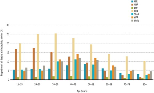
The age-structured models have been studied by many authors, such as Webb [Citation31], Iannelli [Citation16] and Cushing [Citation7]. Age-structured epidemic models were known to be effective tools for studying epidemic dynamics [Citation3–5, Citation17, Citation19, Citation35] and many authors regarded alcoholism as a social epidemic disease [Citation11, Citation30]. According to the WHO report, alcohol-related deaths were related to age (see Figure [1]). Therefore, establishment of alcoholism model should consider age factor and the model becomes more reasonable. However, so far, works on alcoholism models with age structure are very scarce.
Figure 1. Proportion of alcohol-attributable deaths of total deaths by age group, 2012.
In 1990, Thieme [Citation26] observed that age-structured models could be regarded as non-densely defined Cauchy problems, subsequently, Magal and Ruan [Citation22], Liu et al. [Citation18] developed center manifold theory and Hopf bifurcation theorem for non-densely defined Cauchy problems, respectively. By using the above theory and theorem, Liu et al. [Citation20] showed that age-structured model of consumer-resource mutualism exhibited Hopf bifurcation at the positive equilibrium under some conditions. Wang and Liu [Citation29] considered an age-structured compartmental pest-pathogen model. Their results showed that Hopf bifurcation occurred at a positive steady state as bifurcating parameter passed values. Tang and Liu [Citation25] studied a new predator-prey model with age structure and exhibited Hopf bifurcation at a positive steady state.
Motivated by above works, the aim of this paper is to investigate the existence of Hopf bifurcation for an alcoholism model with age-structure. Our model consists of three variables : susceptible drinkers at time t are denoted by , who do not drink or drink only moderately; alcoholics at time t with alcoholism age a are denoted by
, who strongly desire to consume alcohol, having difficulties in controlling of its use, persisting in its use despite harmful consequences; and the people who recover from alcoholism after treatment are denoted by
. Alcoholism as a long-standing social epidemic disease, it is difficult to eliminate for a short time. So we put the alcoholism problem into the population growth model to study. So we suppose new recruits enter the population at a rate
. The population flow among those classes is shown in the following diagram (Figure ).
Figure 2. The flow diagram of our model, where represent
respectively.
![Figure 2. The flow diagram of our model, where [A],[βA] represent ∫0+∞A(t,a)da, ∫0+∞β(a)A(t,a)da, respectively.](/cms/asset/77f12c2b-72b3-4a48-96b6-835940a4966c/tjbd_a_1535668_f0002_oc.jpg)
The flow diagram leads to the following alcoholism model:
(1)
(1) where alcoholics are assumed to be age-structured, whereas susceptible drinkers and recuperator are not age-structured. r is the birth rate, μ is the natural death rate,
are the death rates of excessive drinking, respectively. δ is the transfer rate from alcoholics to recovered individuals, ρ is the relapse rate from recovered individuals to alcoholics. The coefficient α is the fraction of susceptible drinkers
develop into alcoholics because of some of their own reasons, such as losses of earnings, unemployment or family problems, etc. The incidence rate at time t and alcoholism age a is
, where
is the transmission rate due to pressure from alcoholics with alcoholism age a,
is defined by
(2)
(2) and
, i.e.
where τ represents the time span that a person from the initial alcoholism to a potential inviter, who invites susceptible drinkers to increase alcohol consumption. The
represents the total number of secondary alcoholics produced by a primary alcoholic. For the convenience of computation, we assume that
is a constant. The
is the rate that a alcoholic with alcoholism age a
will successfully infect a susceptible drinker.
The remainder of this paper is organized as follows. Section 2, we summarize the main results on Hopf bifurcation theorem, which obtained in [Citation18]. In Section 3, the stability of the steady state and the existence of Hopf bifurcation are investigated. In Section 4, we perform numerical simulations to verify our analytical results. Finally, a brief conclusion is given.
2. Preliminaries
We recall the Hopf bifurcation theorem in Liu et al. [Citation18] for the following non-densely defined abstract Cauchy problem:
(3)
(3) where
is the bifurcation parameter,
is a linear operator on a Banach space X with
not dense in X and A not necessary to be a Hille-Yosida operator,
is a
map with
. Set
and
is the part of A in
, which is defined by
We denote by
the
semigroup of bounded linear operators on X
respectively
the integrated semigroup
generated by A.
Definition 2.1
Let be the infinitesimal generator of a linear
semigroup
on a Banach space X. Define the growth bound
of L by
The essential growth bound
of L by
where
is the space of bounded linear operators from X into X,
is the essential norm of
defined by
, where
, and each bounded set
,
can be covered by a finite number of balls of radius
is the Kuratovsky measure of non-compactness.
We make the following assumptions on the linear operator A and the nonlinear map F.
Assumption 2.1
Assume that is a linear operator on a Banach space
there exist two constants
and
such that
and the following properties are satisfied
.
Assumption 2.1 implies that is the infinitesimal generator of a
-semigroup
on
and
By Proposition 2.6 in Magal and Ruan [Citation22], we know if Assumption 2.1 is satisfied, then A generates a unique integrated semigroup
. If we assume in addition that A is a Hille-Yosida operator, then we have
Next, we consider the non-homogeneous Cauchy problem
(4)
(4) where
.
Assumption 2.2
There exists a map with
such that for each
and
is continuously differentiable and
By Corollary 2.11 in Magal and Ruan [Citation22], we know if Assumption 2.1 and 2.2 hold, then for each ,
, and
, (Equation4
(4)
(4) ) has a unique integrated solution
. Meanwhile, if A is a Hille-Yosida operator, then Assumption 2.8 in [Citation23] holds. By Theorem 2.9 in [Citation23], we know Assumption 2.2 holds.
Assumption 2.3
Let and
for some
. Assume that the following conditions are satisfied:
The essential growth rate of
Base on the above discussion and assumptions, now we can state the following Hopf bifurcation theorem [Citation18].
Theorem 2.1
Let Assumptions 2.1–2.3 be satisfied. Then there exist three
maps,
from
into
from
into
and
from
into
such that for each
there exists a
-periodic function
which is an integrated solution of (2.3) with the parameter value equals
and the initial value equals
. So for each
satisfies
Moreover, we have the following properties
(a) There exist a neighborhood N of 0 in and an open interval I in
containing 0, such that for
and any periodic solution
in N with minimal period
close to
of (2.3) for the parameter value
there exists
such that
(for some
and
(b) The map is a
function and we have the Taylor expansion
where
is the integer part of
.
(c) The period of
is a
function and
where
is the imaginary part of
defined in Assumption 2.3.
3. Stability of equilibria and existence of Hopf bifurcation
In this section, we will study stability of equilibria and existence of Hopf bifurcation for (Equation1(1)
(1) ).
3.1. The transformation of the Cauchy problem
In system (Equation1(1)
(1) ), let
we can rewrite system (Equation1
(1)
(1) ) as the following age-structured model
(5)
(5) where
,
Consider the Banach space
with
Define the linear operator
by
with
we notice L is non-densely defined since
Define the nonlinear operator
by
Set
Now we can rewrite PDEs system (Equation5
(5)
(5) ) as the following non-densely defined abstract Cauchy problem
(6)
(6) The global existence and uniqueness of solutions of system (Equation6
(6)
(6) ) follow from the results of Magal [Citation21] and Magal and Ruan [Citation23].
3.2. Existence of equilibria
If is an equilibrium of (Equation6
(6)
(6) ), we have
which is equivalent to
(7)
(7) Hence we obtain
(8)
(8) where
. From (Equation8
(8)
(8) ) we can get
It is easy to see the system (Equation7
(7)
(7) ) has always trivial equilibrium
Furthermore, if
holds, system (Equation7
(7)
(7) ) has a unique positive equilibrium
where
Lemma 3.1
The system (Equation1(1)
(1) ) has always trivial equilibrium
. If
hold, there exists a unique positive equilibrium of system (Equation1
(1)
(1) )
3.3. Linearized equation
Let , then system (Equation6
(6)
(6) ) is equivalent to the following system
(9)
(9) and the equilibrium
of system (Equation7
(7)
(7) ) is transformed into the zero equilibrium of system (Equation9
(9)
(9) ).
The linearized system of system (Equation9(9)
(9) ) at the equilibrium 0 is as follows
where
. Then system (Equation9
(9)
(9) ) can be written as
where
satisfying
and
.
Denote
By applying the results of Liu, Magal and Ruan [Citation18], we obtain the following result.
Lemma 3.2
For we have the following formula
where
and
.
It is readily checked that
so L is a Hille-Yosida operator and
(10)
(10) Define the part of L in
by
with
and we know
Then, we can claim that
is the infinitesimal generator of a
-semigroup
on
. and for each
the liear operator
is defined by
where
(11)
(11) Now we estimate the essential growth bound of the
semigroup generated by
which is the part of A in
. We observe that for any
,
where
Then
is a compact bounded linear operator. From (Equation10
(10)
(10) ) we obtain
Then we have
By applying the perturbation results in Ducrot, Liu and Magal [Citation6], we obtain
Thus, by the above discussion and Theorem 3.5.5 in [Citation1], we obtain the following proposition.
Proposition 3.1
The linear operator A is a Hille-Yoside operator, and the essential growth rate of the strongly continuous semigroup generated by is strictly negative, that is,
In order to apply Theorem 2.1, we remain to precise the spectral properties of . Setting
and let
. Since
is invertible, it follows that
is invertible if and only if
is invertible. If
is invertible, we obtain
Consider the equation
that is
Then, we obtain the system
this system can be written as
From the formula of
, we know
where
Denote
Then
When
is invertible, we have
From the above discussion and by using the proof of Lemma 3.5 in [Citation29], we obtain the following lemma.
Lemma 3.3
The following results hold:
If
From the above discussion, we know that the linear operator A satisfies Assumptions 2.1–2.3(c) holds.
3.4. Stability of the trivial equilibrium
Now, we consider the stability of the trivial equilibrium we obtain
Thus, we obtain the characteristic equation
where
, and
,
.
It is easy to see that
If
holds, then
has at least one root with a real part. Hence, the equilibrium
is unstable.
If holds, then
by the Routh-Hurwitz criterion, all the roots of
have negative real parts. Hence, the equilibrium
is stable.
Theorem 3.4
If then
is locally asymptotically stable for all
. If
then
is unstable for all
.
Remark 3.1
means
. α is small, then the birth rate r may be less than the mortality rate μ, the whole population is easily extinct. So in reality, the
is more likely to be unstable.
3.5. Stability of the positive equilibrium and Hopf bifurcation
When holds, the characteristic equation of system (Equation1
(1)
(1) ) about the positive equilibrium
can be rewritten as
where
Since
we know the coefficients
have nothing to do with τ.
It is easy to see that
If
, then
Since
By the Routh-Hurwitz criterion, when
all the roots of
have negative real parts if and only if
holds.
If , let
be a purely imaginary roots of
. Then, we have
Separating the real part and the imaginary part in the above equation, we can obtain
(12)
(12) Thus, we have
(13)
(13) i.e.
(14)
(14) Denote
(Equation14
(14)
(14) ) becomes
(15)
(15) Let
and
be three roots of Equation (Equation15
(15)
(15) ). Since
we know
then
it is easy to know that (Equation15
(15)
(15) ) has only one positive real root. We denote this positive real root by
. Then (Equation14
(14)
(14) ) has only one positive real root
.
Let
it is easy to know that
then we have
i.e.
(16)
(16) From (Equation12
(12)
(12) ), we know that
with
has a pair of purely imaginary roots
where
(17)
(17) for
and with
.
Lemma 3.5
Assume that (H1) be satisfied, then
Therefore
is a simple root of
.
Proof.
Differentiating the equation with respect to λ, we have
Thus if
Separating the real part and the imaginary part in the above equation, we can obtain
(18)
(18) Now defining
then
.
According to Equations (Equation12
(12)
(12) ), we know
(19)
(19) With the help of Equations (Equation18
(18)
(18) ) and (Equation19
(19)
(19) ) we deduce that
.
However, thus
This completes the proof.
Lemma 3.6
Assume that (H1) be satisfied, denote the root of
satisfying
where
is defined in (Equation17
(17)
(17) ). Then
Proof.
Taking the derivative of λ with respect to τ in , it is easy to have
By using (Equation13
(13)
(13) ), we obtain
By using (Equation16
(16)
(16) ), it is easy to know that
Noting that
thus
This completes the proof.
Theorem 3.7
Suppose that (H1), (H2) hold, then the following results hold:
If
If
By Theorem 2.1, the above results can be summarized as the following Hopf bifurcation theorem for system (Equation1(1)
(1) )
Theorem 3.8
If (H1) hold. Then there exist where
is defined in (Equation17
(17)
(17) ), such that age-structured acoholism model (Equation1
(1)
(1) ) undergos a Hopf bifurcation at the positive equilibrium
. In particular, when
a non-trivial periodic solution bifurcates from the equilibrium
.
4. Numerical simulations
In this section, we present some numerical simulation to verify the main results by using MATLAB programming. Some of the parameters are taken from [Citation24] . Other parameters are estimated. First, we estimate other parameters as follows
, we can calculate
, by Theorems 3.4 we can expect that the trivial equilibrium
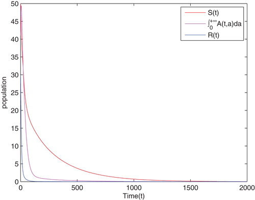
is unstable. see Figure . On the other hand, we estimate other parameters
we can calculate
by Theorems 3.4 we can expect that the trivial equilibrium
is local asymptotically stable. see Figure .
Figure 3. The trajectory of susceptible drinkers , alcoholics
, recuperator
versus time with the initial condition
. When
the equilibrium point
is unstable.

Figure 4. The trajectory of susceptible drinkers , alcoholics
, recuperator
versus time with the initial condition
. When
the equilibrium point
is local asymptotically stable.
Moreover, we estimate other parameters we can calculate
holds, then (Equation1
(1)
(1) ) has only one positive equilibrium
By algorithms in the previous sections, we obtain
and readily checked that the hypothesis of
holds. Thus,
is stable when
, as depicted in Figure . From the numerical simulations we can see the solution of system (Equation1
(1)
(1) ) with the initial condition
and parameter
asymptotically tends to the positive equilibrium
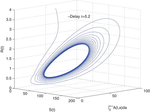
When τ pass through the critical value
,
loss its stability and Hopf bifurcation occurs at
, as depicted in Figure .
Figure 5. The trajectory of susceptible drinkers and recuperator versus time with the initial condition , when
.
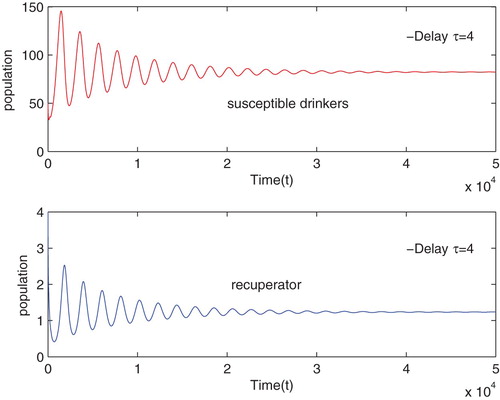
Figure 6. The surface of alcoholics versus time t and age a with the initial condition
, when
.
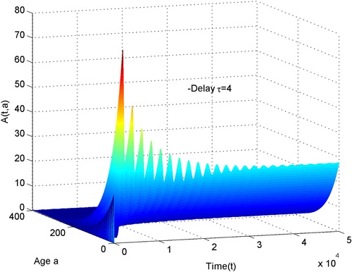
Figure 7. The phase portrait of susceptible drinkers , alcoholics
, recuperator
with the initial condition
, when
.
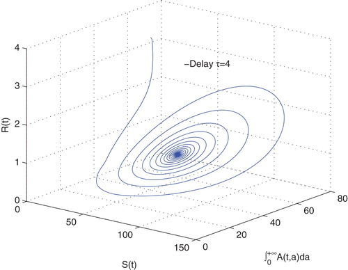
Figure 8. The trajectory of susceptible drinkers and recuperator versus time with the initial condition , when
.
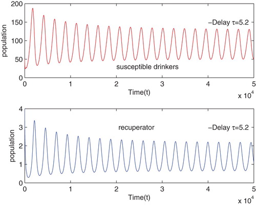
Figure 9. The surface of alcoholics versus time t and age a with the initial condition
, when
.
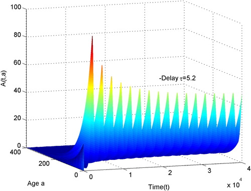
Figure 10. The phase portrait of susceptible drinkers , alcoholics
, recuperator
with the initial condition
, when
.
5. Conclusion
In this paper, Hopf bifurcation of an age-structured alcoholism model is investigated. Real epidemic data indicate regular periodic fluctuations in disease incidence [Citation8–10] but most models for epidemic diseases predict convergence to a unique stable endemic equilibrium, so it is important to examine under what conditions periodic fluctuations in disease incidence can occur. Because there are people who alcoholism for their own reasons, alcoholism, as a social epidemic disease, is somewhat different from common epidemic diseases. However, in our analysis, we found that regular periodic fluctuations can still arise.
By choosing τ as the bifurcation parameter and analyzing the corresponding characteristic equation, we can conclude that the local asymptotically stability of the trivial equilibrium is determined by
. If
, then the trivial equilibrium
is unstable for all
. If
the trivial equilibrium
is local asymptotically stable for all
. For the positive equilibrium, if
holds, we establish conditions to ensure the local stability. The parameter τ does not affect the stability of the trivial equilibrium, but can change the stability of the positive equilibrium. By using the center manifold theory [Citation22] and Hopf bifurcation theorem [Citation18], which developed for non-densely defined Cauchy problems, the existence of Hopf bifurcation at the positive equilibrium is obtained. In particular, a non-trivial periodic solution bifurcates from the positive equilibrium when bifurcation parameter τ passes through the critical values
. Our analytical results indicate that introduction of parameter τ can affect the dynamic behavior of the system (Equation1
(1)
(1) ).
Moreover, due to alcoholism is often associated with some of the alcoholics' own reasons, such as losses of earnings, unemployment or family problems, etc. In this sense, as long as the population is not extinct (according to the analysis of Remark 3.1, the is more likely to be unstable), alcoholics will always exist. Therefore, we hope that alcohol-attributable socioeconomic burden is minimal. This optimal control problem, we will study in future work.
Disclosure statement
No potential conflict of interest was reported by the authors.
Additional information
Funding
References
- W. Arendt, C. Batty, M. Hieber, and F. Neubrander, Vector-Valued Laplace Transforms and Cauchy Problems, Birkhäser Verlag, Basel, 2001.
- Y. Cai, J. Jiao, Z. Gui, Y. Liu, and W. Wang, Environmental variability in a stochastic epidemic model, Appl. Math. Comput. 329 (2018), pp. 210–226.
- Y. Chen, S. Zou, and J. Yang, Global analysis of an SIR epidemic model with infection age and saturated incidence, Nonlinear Anal. 30 (2016), pp. 16–31. doi: 10.1016/j.nonrwa.2015.11.001
- X. Duan, S. Yuan, and X. Li, Global stability of an SVIR model with age of vaccination, Appl. Math. Comput. 226 (2014), pp. 528–540.
- X. Duan, S. Yuan, Z. Qiu, and J. Ma, Global stability of an SVEIR epidemic model with ages of vaccination and latency, Comput. Math. Appl. 68(3) (2014), pp. 288–308. doi: 10.1016/j.camwa.2014.06.002
- A. Ducrot, Z. Liu, and P. Magal, Essential growth rate for bounded linear perturbation of non densely defined cauchy problems, J. Math. Anal. Appl. 341(1) (2008), pp. 501–518. doi: 10.1016/j.jmaa.2007.09.074
- J. Cushing, An Introduction to Structured Population Dynamics, Society for Industrial and Applied Mathematics, Philadelphia, PA, 1998.
- P.E.M. Fine and J.A. Clarkson, Measles in england and wales I: An analysis of factors underlying seasonal patterns, Int. J. Epidemiol. 11(1) (1982), pp. 5–14. doi: 10.1093/ije/11.1.5
- P.E.M. Fine and J.A. Clarkson, Measles in england and wales II. The impact of the measles vaccination programme on the distribution of immunity in the population, Int. J. Epidemiol. 11(1) (1982), pp. 15–25. doi: 10.1093/ije/11.1.15
- P.E.M. Fine and J.A. Clarkson, Measles in england and wales III. Assessing published predictions of the impact of vaccination of incidence, Int. J. Epidemiol. 12(3) (1983), pp. 332–339. doi: 10.1093/ije/12.3.332
- H.F. Huo and X.M. Zhang, Complex dynamics in an alcoholism model with the impact of twitter, Math. Biosci. 281 (2016), pp. 24–35. doi: 10.1016/j.mbs.2016.08.009
- H.F. Huo, R. Chen, and X.Y. Wang, Modelling and stability of hiv/aids epidemic model with treatment, Appl. Math. Model. 40 (2016), pp. 6550–6559. doi: 10.1016/j.apm.2016.01.054
- H.F. Huo, S.R. Huang, X.Y. Wang, and H. Xiang, Optimal control of a social epidemic model with media coverage, J. Biol. Dyn. 11 (2017), pp. 226–243. doi: 10.1080/17513758.2017.1321792
- H.F. Huo, Y.L. Chen, and H. Xiang, Stability of a binge drinking model with delay, J. Biol. Dyn. 11 (2017), pp. 210–225. doi: 10.1080/17513758.2017.1301579
- H.F. Huo, F.F. Cui, and H. Xiang, Dynamics of an saits alcoholism model on unweighted and weighted networks, Phys. A 496 (2018), pp. 249–262. doi: 10.1016/j.physa.2018.01.003
- M. Iannelli, Mathematical Theory of Age-Structured Population Dynamics, Giadini Editori e Stampatori, Pisa, 1994.
- X.Z. Li, J. Wang, and M. Ghosh, Stability and bifurcation of an SIVS epidemic model with treatment and age of vaccination, Appl. Math. Model. 34(2) (2010), pp. 437–450. doi: 10.1016/j.apm.2009.06.002
- Z. Liu, P. Magal, and S. Ruan, Hopf bifurcation for non-densely defined cauchy problems, Z. Angew. Math. Phys. 62(2) (2011), pp. 191–222. doi: 10.1007/s00033-010-0088-x
- L. Liu, J. Wang, and X. Liu, Global stability of an SEIR epidemic model with age-dependent latency and relapse, Nonlinear Anal. 24 (2015), pp. 18–35. doi: 10.1016/j.nonrwa.2015.01.001
- Z. Liu, P. Magal, and S. Ruan, Oscillations in age-structured models of consumer-resource mutualisms, Discrete Contin. Dyn. Syst. Ser. B 21(2) (2016), pp. 537–555. doi: 10.3934/dcdsb.2016.21.537
- P. Magal, Compact attractors for time-periodic age structured population models, Electron. J. Differential Equations 2001(65) (2001), pp. 1–35.
- P. Magal, S. Ruan. Center manifolds for semilinear equations with non-dense domain and applications on hopf bifurcation in age structured models, Mem. Amer. Math. Soc. 202(2009), pp. 1–67. No. 951.
- P. Magal and S. Ruan, On semilinear cauchy problems with non-dense domain, Adv. Differential Equations 14(11–12) (2009), pp. 1041–1084.
- G. Mulone and B. Straughan, Modeling binge drinking, Int. J. Biomath. 5(1) (2012), p. 1250005. doi: 10.1142/S1793524511001453
- H. Tang and Z. Liu, Hopf bifurcation for a predator-prey model with age structure, Appl. Math. Model. 40(2) (2016), pp. 726–737. doi: 10.1016/j.apm.2015.09.015
- H.R. Thieme, Semiflows generated by lipschitz perturbations of non-densely defined operators, Differential Integral Equations 3(6) (1990), pp. 1035–1066.
- G. Thomas and E.M. Lungu, A two-sex model for the influence of heavy alcohol consumption on the spread of HIV/AIDS, Math. Biosci. Eng. 7(4) (2010), pp. 871–904. doi: 10.3934/mbe.2010.7.871
- W. H. Organization, Global status report on alcohol and health, 2014.
- Z. Wang and Z. Liu, Hopf bifurcation of an age-structured compartmental pest-pathogen model, J. Math. Anal. Appl. 385(2) (2012), pp. 1134–1150. doi: 10.1016/j.jmaa.2011.07.038
- X.-Y. Wang, K. Hattaf, H.-F. Huo, and H. Xiang, Stability analysis of a delayed social epidemics model with general contact rate and its optimal control, J. Ind. Manag. Optim. 12(4) (2016), pp. 1267–1285. doi: 10.3934/jimo.2016.12.1267
- G. Webb, Theory of Nonlinear Age-Dependent Population Dynamics, Marcel Dekker, New York, NY, 1985.
- H. Xiang, N.N. Song, and H.F. Feng, Modelling effects of public health educational campaigns on drinking dynamics, J. Biol. Dyn. 10(1) (2016), pp. 164–178. doi: 10.1080/17513758.2015.1115562
- H. Xiang, Y.L. Tang, and H.F. Huo, A viral model with intracellular delay and humoral immunity, Bull. Malays. Math. Sci. Soc. 40 (2017), pp. 1011–1023. doi: 10.1007/s40840-016-0326-2
- H. Xiang, Y.-P. Liu, and H.-F. Huo, Stability of an SAIRS alcoholism model on scale-free networks, Phys. A 473 (2017), pp. 276–292. doi: 10.1016/j.physa.2017.01.012
- J. Yang, Y. Chen, and F. Xu, Effect of infection age on an SIS epidemic model on complex networks, J. Math. Biol. 73(5) (2016), pp. 1227–1249. doi: 10.1007/s00285-016-0991-7