
 ?Mathematical formulae have been encoded as MathML and are displayed in this HTML version using MathJax in order to improve their display. Uncheck the box to turn MathJax off. This feature requires Javascript. Click on a formula to zoom.
ABSTRACT
We use a general autonomous discrete-time infectious disease model to extend the next generation matrix approach for calculating the basic reproduction number, , to account for populations with locally asymptotically stable period k cycles in the disease-free systems, where
. When
and the demographic equation (in the absence of the disease) has a locally asymptotically stable period k population cycle, we prove the local asymptotic stability of the disease-free period k cycle. That is, the disease goes extinct whenever
. Under the same period k demographic assumption but with
, we prove that the disease-free period k population cycle is unstable and the disease persists. Using the Ricker recruitment function, we apply our results to discrete-time infectious disease models that are formulated for Susceptible-Infectious-Recovered (SIR) infections with and without vaccination, and Infectious Salmon Anemia Virus (ISA
) infections in a salmon population. When
, our simulations show that the disease-free period k cycle dynamics drives the SIR disease dynamics, but not the ISAv disease dynamics.
1. Introduction
The next generation matrix approach for calculating the basic reproduction number, , has been very useful in determining biologically meaningful thresholds for guaranteeing local stability (disease extinction) or instability (disease persistence) of the disease-free equilibrium of infectious disease epidemic models [Citation2,Citation7,Citation8,Citation10,Citation18,Citation25,Citation26]. For autonomous infectious disease models (without seasonality or periodicity), the next generation matrix approach assumes the existence of a locally asymptotically stable disease-free equilibrium in the demographic equation. That is, in the absence of the disease, the population is assumed to be at a static steady state [Citation2,Citation7,Citation10]. However, density dependent birth or recruitment functions, such as the Ricker or Quadratic discrete-time models, are known to generate locally asymptotically periodic (cyclic) or erratic (chaotic) fluctuations in autonomous disease-free demographic equations, where the static equilibrium point is unstable [Citation20]. Such prominent and persistent cyclic fluctuations have been observed in the abundance of some sockeye salmon populations [Citation17], and the Ricker model was first used to study population cycles in fish [Citation22]. Some mammals in high northern latitudes, for example snowshoe hares (Lepus americanus), show regular population cycles. Herbivores with high-amplitude population cycles, such as voles, lemmings, snowshoe hares and forest Lepidoptera, form the heart of terrestrial food web dynamics. Also, red grouse populations in Britain exhibit cyclic fluctuations in abundance, with periodic crashes [Citation14,Citation23].
In this paper, we use a general autonomous discrete-time epidemic model to extend the next generation matrix approach for calculating the basic reproduction number, , to account for populations with periodic demographic dynamics. In these models, the basic reproduction number determines local stability
or instability of the extinction periodic cycle
, where the disease-free dynamics is locally asymptotically periodic. We apply the extended next generation matrix approach for calculating
to two discrete-time epidemic models with Ricker recruitment functions, a Susceptible - Infectious - Recovered (SIR) model with and without vaccination, and an Infectious Salmon Anemia Virus (ISA
) model.
In the SIR model, the dynamics of the Ricker demographic equation in the absence of the disease is qualitatively equivalent to the dynamics of the total population, . However, in the ISA
model, the dynamics of the salmon population equation in the absence of the disease is qualitatively different from that of the total salmon population,
. As a result, when
, the period of the disease-free susceptible population cycle in the SIR model is numerically found to determine the period of the infectious population cycle. However, in the ISA
model, the period of the infectious salmon population can be different from that of the disease-free salmon population. In particular, the ISA
disease is capable of forcing population fluctuations in the salmon population (see Figure ).
Others have computed for time-periodic (nonautonomous) discrete-time and continuous-time disease epidemic models (for example, see [Citation3] and the references therein). The discrete-time autonomous epidemic models for this study are not seasonal or time-periodic. Our model's demographic population cycles are forced by the density-dependent one-hump Ricker recruitment function via period-doubling bifurcations route to chaos [Citation6,Citation11,Citation12,Citation22,Citation26,Citation29].
In Section 2, we derive the next generation matrix method for calculating in autonomous discrete-time epidemic models with demographic population cycles. To demonstrate how the results of Section 2 can be applied to study specific autonomous discrete-time diseases with demographic population cycles, we introduce SIR and ISA
disease models in Sections 3 and 4, respectively. For each of these models, we compute
and use it to establish disease persistence and extinction. In Section 3, we compute a vaccination reproduction number,
and use it to determine how adopting a vaccination control policy in the cyclic environment lowers the values of
. Our simulations, Figure in Section 3 and Figure in Section 4, illustrate the relationship between
and the infectious population cycles. We summarize our results in the Concluding Remarks section.
2. Next generation matrix method and demographic population cycles
A next generation matrix method for computing the basic reproduction number, for discrete-time compartmental epidemic models with a stable fixed point was developed by Allen and van den Driessche in Theorem 2.1 of [Citation2]; see also Theorem 3.3 in Li and Schneider [Citation18] and Theorem 3 in Cushing and Yicang [Citation8]. As in [Citation2], to describe the method for
when the disease-free dynamics is a period k population cycle, for
and
, we write a general discrete-time compartmental infectious disease model in the form
(1)
(1) where
and
. Thus, Model (Equation1
(1)
(1) ) describes the disease dynamics of the states of the population over discrete-time intervals. Suppose that m<n and the states are ordered so that at generation
, the first m states, denoted as
, are the infectious states, and the remaining n−m states are the healthy noninfectious states, denoted as
. Hence, as in [Citation2], Model (Equation1
(1)
(1) ) can be written as the following system of difference equations.
(2)
(2) Using knowledge of vectors of population sizes in the disease and non-disease compartments,
and
, at time t, Model (Equation2
(2)
(2) ) predicts the vectors of population sizes in the disease and non-disease compartments,
and
, at time
, where
. The specific model's unit of time depend on the disease application. For example, the unit of time could be a convenient time for a follow up census. The basic reproduction number,
, the lifetime production of infections produced per infectious individual, is independent of the model's time scale. We will use Model (Equation2
(2)
(2) ) to compute
when the demographic population dynamics is oscillatory with period k population cycle.
We assume that the disease-free system has a unique positive disease-free period k population cycle at , where
, and for
and
. In addition, we assume that linearization of Model (Equation1
(1)
(1) ) about the disease-free period k population cycle yields the linearized system
(3)
(3) where for each
,
is the
Jacobian matrix of Model (Equation1
(1)
(1) ) evaluated at the disease-free period k cycle. For each
,
has the following form:
(4)
(4) where the
submatrices
and
are nonnegative and O is the zero matrix. Each matrix,
and
is obtained from differentiation with respect to states
and evaluated at the disease-free k cycle,
. As in [Citation2], by letting
, where
is the vector of new infections that survive the time interval and
is the vector of all the other transitions, we respectively obtain
and
. Thus, for each
,
is the matrix of new infections and
is the transition matrix. Since some of the population may die either from the disease infection or natural causes during the k−cycle, we assume that the spectral radius of the product of the k transition matrices,
, is less than 1.
The linearized system reduces to the following form:
(5)
(5) In the disease-free state, we assume that disease-free period k cycle is locally asymptotically stable. That is, the spectral radius of the product matrix,
, is less than one. Therefore, we assume
(6)
(6) Notice that the matrix in (Equation5
(5)
(5) ) is a block matrix with
. Consequently, the stability of the linearized system, (Equation5
(5)
(5) ), depends on the eigenvalues of the product matrix
, and is independent of the matrix
. To provide a definition for the basic reproduction,
we let
and
Then
The product matrices,
and
are entrywise non-negative. That is,
and
. We assume that,
is irreducible. Furthermore, along the period k population cycle,
is the effective matrix of new infections and
is the transition matrix. Since
and
, it follows that
where Id is an
identity matrix. Thus,
is entrywise non-negative. Let
be the number of initially infected individuals. Then
is an entrywise non-negative vector that gives the expected number of new infections over the period k population cycle. The matrix
has
entry equal to the expected number of secondary infections in compartment i produced by an infected individual introduced in compartment j. Consequently, when the disease-free system has a unique positive locally asymptotically stable disease-free period k population cycle, the matrix
is the next generation matrix, and the basic reproduction number is
Using the above periodic next generation matrix method notation, we summarize the relationship between the unique positive disease-free period k population cycle at
, and
in the following result.
Theorem 2.1
If is a disease-free period k population cycle of the system
then
is locally asymptotically stable if
but unstable if
where using the above notation
is irreducible and
.
The proof of Theorem 2.1 is similar to that of Theorem 2.1 in [Citation2] and is omitted. When the disease-free system has a unique locally asymptotically stable disease-free equilibrium (fixed point), then k=1 and reduces to
[Citation2]. In a recent paper, van den Driessche and Yakubu [Citation26], proved that when
and the demographic dynamics is asymptotically constant or under geometric growth (non-oscillatory), then the disease-free equilibrium point (fixed point) is globally asymptotically stable. Can a disease-free population cycle with period
be globally asymptotically stable? This question was answered in 2002 by Elaydi and Yakubu who showed that this is not possible in autonomous discrete-time models such as Model (Equation1
(1)
(1) ) ([Citation12], Theorem 3).
3. SIR model with demographic population cycles
Susceptible - Infectious - Recovered (SIR) disease epidemic models have been used to study childhood diseases including chicken pox (varicella) and for the host population in the study of vector borne diseases (for example, malaria) [Citation4,Citation5,Citation19,Citation25]. To introduce a SIR disease epidemic model with periodic demographic dynamics, we assume that at each generation , each member of a population is either susceptible (
), infectious (infected with the disease,
) or recovered from the disease with life-long immunity (
), where the total population is
That is, we let
,
,
and
, respectively denote the population density of susceptible, infectious, recovered and total population of individuals at time
.
Following Yakubu [Citation29] and the references therein, we assume that susceptible individuals who interact with infectious individuals become infectious with probability and remain susceptible with probability
per unit time interval, where the ‘escape’ function
is a nonlinear decreasing smooth concave up function with
. That is,
and
for all
. For example, when infections are modelled as Poisson processes, then
with the transmission constant
.
Furthermore, we assume that infectious individuals recover from the infection with constant probability and remain infectious with constant probability
per generation. We assume that the probability of natural death for each individual in the population is
per generation, and probability of staying alive per generation is
. We assume that a susceptible individual has to be in the infectious class before recovering, and recovered individuals have life-long immunity. That is, we consider a disease that is not fatal so we ignore death due to the disease.
To include periodic demography dynamics, we let
denote the nonlinear differentiable recruitment (birth or immigration) function of individuals to the susceptible class per unit time interval, where
. The Ricker recruitment function,
is an example of the recruitment function for this study, with the intrinsic growth rate r>0 and the scaling parameter b>0.
Our discrete-time SIR model with mass action type incidence, , implicitly assumes three distinct temporal phases. At the end of each generation, susceptibles become infectious while infectious recover; a fraction of each class is removed; then susceptibles, infectious and recovered reproduce into the susceptible class. These important assumptions distinguish our discrete-time SIR epidemic model from a similar continuous-time differential equation model. Typically, continuous-time differential equation models with similar well-defined distinct temporal phases are non-autonomous. Taking into account the temporal ordering of events, as in [Citation26], we derive our SIR model in the following three steps.
Disease Transmission and Recovery:
That is, after disease transmission and recovery,
Natural Death (Survival):
Reproduction or recruitment (S, E, I and R into S):
These assumptions and notation lead to the following discrete-time SIR epidemic model.
(7)
(7) where
. We study Model (Equation7
(7)
(7) ) with initial conditions
. Note that in Model (Equation7
(7)
(7) ), we assume that events happen in the following order: disease transmission and recovery, survival (death) and reproduction or recruitment. However, in real biological systems, these three events may happen in different orders.
Theorem 3.1
In Model (Equation7(7)
(7) ), for each time
and there is no population explosion whenever
.
Proof.
Since , each equation of Model (Equation7
(7)
(7) ) is a sum of nonnegative terms. Hence,
for all
. Next, we prove boundedness of orbits. Summing all the three equations of Model (Equation7
(7)
(7) ), at each time
, the total population is governed by the demographic equation
and
. Since,
is smooth and
there exists K>0 and
such that
for all
. Thus,
, the set of iterates of all non-negative initial population sizes are bounded and there is no population explosion in Model (Equation7
(7)
(7) ).
At each time , when
, Model (Equation7
(7)
(7) ) reduces to the following disease-free equation.
(8)
(8) Since
, Model (Equation7
(7)
(7) ) and Equation (Equation8
(8)
(8) ) respectively have the trivial equilibrium,
and
. To include periodic demography dynamics in Model (Equation7
(7)
(7) ), we assume that the demographic Equation (Equation8
(8)
(8) ) has a unique positive locally asymptotically stable period k population cycle at
, where
. That is, in Model (Equation8
(8)
(8) ) we assume that
exists and
(9)
(9) where
.
3.1. for SIR model with demographic population cycles
To compute the basic reproduction number, , for Model (Equation7
(7)
(7) ) by the next generation matrix method, for each
,
where the demographic Equation (Equation8
(8)
(8) ) is assumed to have a unique positive locally asymptotically stable period k population cycle. Hence, the transition matrix is
and the matrix of new infections is
For this model, the matrices
and
are positive scalars, and
. Hence,
By Theorem 2.1, the disease-free period k population cycle in Model (Equation7
(7)
(7) ) is locally asymptotically stable when
and unstable when
. When d=0 (no death) and k=1 in Model (Equation7
(7)
(7) ), it becomes a simple SIR model with fixed point (non-oscillatory) dynamics, and
reduces to
.
Next, we consider an extension of Model (Equation7(7)
(7) ). Suppose that a fraction p of individuals are vaccinated at recruitment into the susceptible population. Furthermore, suppose that the vaccine is perfectly effective, so everyone receiving the vaccine is protected from the infection. We assume that
enter the S compartment and the remaining
enter the recovered compartment. Then Model (Equation7
(7)
(7) ) becomes
(10)
(10) The following system is the disease-free system for Model (Equation10
(10)
(10) ).
(11)
(11) Model (Equation11
(11)
(11) ) has a trivial DFE,
. Summing the equations for
and
in Model (Equation11
(11)
(11) ) results in the following one-dimensional equation in
.
(12)
(12) Equation (Equation12
(12)
(12) ) is similar to (Equation8
(8)
(8) ). By assumption, Equations (Equation8
(8)
(8) ) and (Equation12
(12)
(12) ) have the unique positive locally asymptotically stable period k population cycle,
. Consequently, the disease-free system with vaccination, Model (Equation11
(11)
(11) ), has the unique positive period k population cycle,
In Model (Equation11
(11)
(11) ) we assume that
is locally asymptotically stable. That is,
(13)
(13) where
for each
.
It is possible for to be a locally asymptotically stable period k population cycle of Model (Equation11
(11)
(11) ), where
is a locally asymptotically stable period k population cycle of Model (Equation8
(8)
(8) ) or (Equation12
(12)
(12) ). In the following result, we illustrate this possibility when k=1.
Proposition 3.2
Let be a positive fixed point of Model (Equation8
(8)
(8) ) or (Equation12
(12)
(12) ), where
Then
is a locally asymptotically stable fixed point of Model (Equation8
(8)
(8) ) or (Equation12
(12)
(12) ), and
is a locally asymptotically stable positive fixed point of Model (Equation11
(11)
(11) ).
Proof.
Since ,
is a locally asymptotically fixed point of Model (Equation8
(8)
(8) ) or (Equation12
(12)
(12) ). Clearly,
is a positive fixed point of Model (Equation11
(11)
(11) ). Next, we use a local stability analysis to determine the stability of
. The Jacobian matrix of Model (Equation11
(11)
(11) ) evaluated at
is
Thus,
By assumption,
. Hence,
. That is,
. Also,
implies that
Determinant
. Consequently,
and by the Jury test,
is a locally asymptotically stable positive fixed point of Model (Equation11
(11)
(11) ).
The vaccination reproduction number, also called a control reproduction number, denoted by , is given by
(14)
(14) Notice that
, and adopting a vaccination policy decreases the reproduction number. As in Model (Equation7
(7)
(7) ), the disease-free population cycle of Model (Equation10
(10)
(10) ) with vaccination,
is locally asymptotically stable and the disease goes extinct when
. However,
is unstable and the disease persists when
.
When the disease-free system without vaccination, (Equation8(8)
(8) ), has the unique positive equilibrium point,
, and
, then by Proposition 3.2,
and
are locally asymptotically stable equilibrium points of Models (Equation8
(8)
(8) ) and (Equation11
(11)
(11) ) respectively. In this case,
To bring
below the threshold value 1, the fraction that needs to be vaccinated to give herd immunity is known to be
. In the next section, we will use the Ricker recruitment function and demographic population cycles in Model (Equation10
(10)
(10) ) to determine how to bring
below the threshold value 1, where
.
3.2. Ricker recruitment function
The Ricker model was first used to model fish populations. However, it is used in theoretical ecology and epidemiology to model all types of population dynamics and recruitment functions [Citation6,Citation11,Citation12,Citation22,Citation26,Citation29]. When the recruitment function is the Ricker Model, , the disease-free Equation (Equation8
(8)
(8) ) without vaccination reduces to
(15)
(15) In this case,
. Let
Then, in the absence of the disease the susceptible population goes extinct when
. However, when
the disease-free population persists on a fixed point or cyclic or chaotic attractor. When
, the disease-free system persists on the fixed point attractor,
. When
, then the disease-free Equation (Equation8
(8)
(8) ) is known to undergo period-doubling bifurcations route to chaos [Citation6,Citation11,Citation12,Citation26]. Typically, populations that exhibit periodic cycles take on their highest and lowest population sizes at regular time intervals. To illustrate population cycles in (Equation8
(8)
(8) ), we choose the probability of natural death to be equal to the probability of staying alive per generation so that d=0.5. To scale the population sizes, we choose the scaling parameter, b, to equal 0.1. In Figure , we illustrate period-doubling bifurcations in the disease-free Equation (Equation8
(8)
(8) ) as the intrinsic growth rate, r, is varied between 20 and 140, where d=0.5 and b=0.1. With our choice of parameters, (Equation15
(15)
(15) ) has an asymptotically stable fixed point when
, and the fixed point undergoes period-doubling bifurcation at
. Figure shows windows of population cycles of period
, and the range of the values of the parameter r for the local asymptotic stability of the periodic population cycles.
Figure 1. Period-doubling bifurcations in the disease-free Equation (Equation15(15)
(15) ), where d=0.5, b=0.1, on the horizontal axis
and on the vertical axis
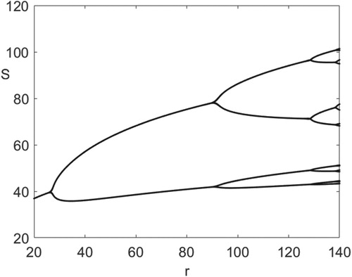
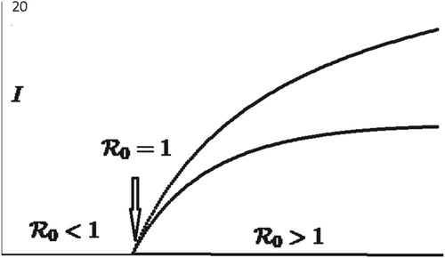
Figure 2. Bifurcation diagram for SIR model: As increases from values less than 1 to values greater than 1, the model dynamics changes from disease extinction to disease persistence on a locally asymptotically stable period 2 population cycle.
From Figure , the disease-free Equation (Equation15(15)
(15) ) exhibits a locally asymptotically stable period 2 population cycle at
(16)
(16) when
, and a locally asymptotically stable period 4 population cycle at
(17)
(17) when
.
3.3. SIR model with Ricker recruitment function
Now, we consider Model (Equation7(7)
(7) ) with
, where the model's unit of time is a year. To compute
for this example, as in [Citation6] and [Citation26], we assume that the SIR disease infections are modelled as Poisson processes with
where
. When the disease-free system has a locally asymptotically stable period 2 population cycle,
, then
(18)
(18) To illustrate the impact of increasing
from values less than 1 to values greater than 1 on Model (Equation7
(7)
(7) ) with
, let
while β varies between 0 and 0.1. From (Equation16
(16)
(16) ), with our choice of parameters, the disease-free Equation (Equation8
(8)
(8) ) has a locally asymptotically stable period 2 population cycle at
. Furthermore, as the infection rate β increases from zero to values greater than
,
increases from values less than 1 (disease extinction, see Figure ) to values greater than 1 (disease persistence on a period 2 population cycle, see Figure ). As predicted by Theorem 2.1, Figure shows that the disease-free period 2 population cycle is locally asymptotically stable when
and unstable when
.
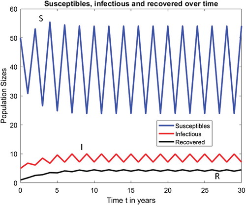
For example, when all parameters are kept fixed at their current values and , then
and Figures and show that Model (Equation7
(7)
(7) ) with
has a locally asymptotically stable endemic period 2 population cycle at
Figure 3. Model (Equation7(7)
(7) ) with
has a locally asymptotically stable endemic period-2 population cycle when
.
3.4. Vaccination in SIR model with ricker recruitment function
In this section, we consider Model (Equation10(10)
(10) ) with the Ricker recruitment function
. The disease-free Model (Equation11
(11)
(11) ) becomes
(19)
(19) The population dynamics of Model (Equation19
(19)
(19) ) is similar to that of Equation (Equation15
(15)
(15) ). As in Equation (Equation15
(15)
(15) ), the trivial disease-free equilibrium of Model (Equation19
(19)
(19) ),
, is globally asymptotically stable and the population goes extinct when
. However,
is unstable, and the disease-free population persists when
. When
, as in the one-dimensional disease-free system without vaccination, the disease-free population of Model (Equation19
(19)
(19) ) persists on the fixed point attractor,
. When
, as in Equation (Equation15
(15)
(15) ), the positive fixed point of the 2-dimensional Model (Equation19
(19)
(19) ) undergoes period-doubling bifurcations route to chaos [Citation6,Citation11,Citation12,Citation26]. To illustrate this Equation (Equation15
(15)
(15) ) induced period-doubling bifurcations in Model (Equation19
(19)
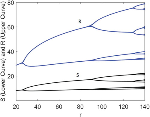
(19) ), set p=0.78 and keep all the other parameters fixed at their current values in Figure . As in Figure , Figure shows that, under a vaccination programme, both the susceptible and recovered disease-free populations undergo period-doubling bifurcations as r is varied between 20 and 140, where d=0.5 and b=0.1. That is, the population dynamics of the one-dimensional disease-free model without vaccination determines qualitatively the dynamics of the two-dimensional disease-free system with vaccination (bifurcation points of the two models are the same but S values are lower with the vaccination at p=0.78).
Figure 4. Susceptible and recovered disease-free populations of Model (Equation19(19)
(19) ) undergo period-doubling bifurcations as r is varied between 20 and 140, where p=0.78, d=0.5 and b=0.1.
When
in Model (Equation7
(7)
(7) ) with
and no vaccination
, then
where the period of the disease-free population is 2 (see Equation (Equation18
(18)
(18) ) in Section 3.3 for
formula). However, keeping all the parameters fixed at their current values, and introducing vaccination at p=0.78 decreases the reproduction number to
, from Equation (Equation14
(14)
(14) ) in Section 3.1. That is, as in populations with non periodic demographic dynamics, vaccination programmes can play a role in controlling infectious diseases in populations with periodic demographic dynamics.
4. ISAv model with demographic population cycles
Infectious salmon anemia (ISA), a finfish disease caused by a virus that belongs to a family of viruses called Orthomyxoviridae, has caused significant mortality among salmon farms in Northern Europe, Canada, Maine, and Chile. Worldwide, economic losses due to ISA have been in the billions of dollars. Due to the severity of ISA, the European Union includes infectious salmon anemia in its list of the most dangerous diseases of fish, and it is one of just 10 virus infections of finfish that is reportable to the World Organization for Animal Health [Citation9,Citation15,Citation21,Citation28]. Currently, there are no treatment options available for ISA. Typically, ISAv disease outbreaks have been managed through a combination of regulatory measures and husbandry practices, including restricted movements of fish between farms, enforced slaughtering, use of all-in–all-out programmes at farms, and disinfection of slaughterhouses and processing plants. ISAv vaccine preparations provide partial protection, but their use is limited by difficulties associated with vaccine delivery to large numbers of fish [Citation13,Citation16,Citation21,Citation27].
In [Citation21], Milliken and Pilyugin introduced a two-patch (migration-linked farm and wild salmon populations) ordinary differential equations model of infectious salmon anemia virus with logistic growth. Here, we introduce a single patch discrete-time ISAv model with Ricker stock recruitment, which has been used to describe stock and recruitment in fisheries [Citation22]. As in [Citation21], we assume that at each time , each live salmon is either susceptible,
or infectious (infected with ISA disease),
. That is, we let
,
, and
=
+
respectively denote the population size of susceptible, infectious, and total population of live salmon at each time t. Once infected, salmon do not recover from the ISAv disease. Thus, we use an SI epidemic model with no recovery class to describe the salmon population [Citation1]. At each time
, we denote the virus population size by
.
We assume that the susceptible salmon population experiences Ricker growth. As in [Citation21], we assume that infected salmon cannot reproduce. The intrinsic birth rate of salmon per time interval is denoted by r>0. Consequently, assuming all newborn salmon are susceptible,
where the scaling parameter b>0. Also, per unit time interval,
is the fraction of salmon that die ‘naturally’,
is the fraction of salmon that survive,
is the constant ISA induced mortality,
is the fraction of ISA infectious salmon that survive,
is the constant fraction of virus that is cleared and
is the fraction of virus that survive.
At each time we assume that a fraction of susceptible salmon,
, become infected from direct contact with infectious salmon with probability
, and the remaining susceptible salmon,
, become infected via contact with the ISA virus with probability
, where the ‘escape’ functions
are nonlinear decreasing smooth concave up functions with
,
,
,
and
. For example, when ISAv infections are modelled as Poisson processes, then
and
with the transmission constants
,
. As in [Citation21], we account for virus shedding in our model. During each time interval,
is the population of virus shed, where
.
As in Model (Equation7(7)
(7) ), our discrete-time ISAv model implicitly assumes three distinct temporal phases. At the end of each time interval, susceptible salmon populations become infectious, a fraction of infectious salmon die, shedding occurs; a fraction of each salmon class is removed (natural death and virus clearing); and susceptible salmon populations reproduce into the susceptible class. Taking into account the temporal ordering of events, we derive our ISAv model in the following three steps.
Disease transmission, disease induced death, and shedding:
Natural Death (salmon survival and virus clearing):
Reproduction or Ricker recruitment (S into S):
These assumptions and notation lead to the following discrete-time ISAv epidemic model.
(20)
(20) where
. We study Model (Equation20
(20)
(20) ) with initial conditions
.
Theorem 4.1
In Model (Equation20(20)
(20) ), for each time
and there is no population explosion whenever
Proof.
Clearly, implies
for each time
. From the equation of
and the susceptible salmon population is bounded. Furthermore, from the equations of
Using the boundedness of the susceptible salmon population, we obtain that the infectious salmon population is also bounded. Hence, there is no population explosion in the salmon population of Model (Equation20
(20)
(20) ). From the equation of
, the virus population is also bounded. Hence, the set of iterates of all non-negative initial population sizes are bounded and there is no population explosion in Model (Equation20
(20)
(20) ).
At each time , when there is no ISAv disease and
, Model (Equation20
(20)
(20) ) reduces to Model (Equation15
(15)
(15) ). Notice that when the salmon population of Model (Equation20
(20)
(20) ) is missing, the virus population decreases to zero. Consequently,
implies extinction of the salmon and virus populations in Model (Equation20
(20)
(20) ). However,
implies persistence of the salmon population, and the demographic Equation (Equation15
(15)
(15) ) has a unique positive locally asymptotically stable period k salmon population cycle
, where
4.1. for ISAv model
Assuming virus shedding is not a new infection, we compute the basic reproduction number, , for Model (Equation20
(20)
(20) ) by the next generation matrix method, as in Section 3.1. For each
,
and
where the salmon demographic threshold
and Equation (Equation15
(15)
(15) ) has a unique positive locally asymptotically stable period k salmon population cycle. Hence, the nonnegative transition matrix is
with
, and the nonnegative matrix of new infections is
where
is irreducible. Consequently, the basic reproduction number for Model (Equation20
(20)
(20) ) is
when
and Equation (Equation15
(15)
(15) ) has a unique positive locally asymptotically stable period k salmon population cycle. By Theorem 2.1, when
the positive disease-free period k salmon population cycle in Model (Equation20
(20)
(20) ) is locally asymptotically stable when
and unstable when
.
When , the disease-free system persists on a fixed point attractor
non-oscillatory
, and Equation (Equation15
(15)
(15) ) has a positive locally asymptotically stable fixed point salmon population (k=1),
. Assuming that virus shedding is not a new infection, and proceeding exactly as before we obtain that at the DFE,
, the matrix of new infections that survive the time interval is
the transition matrix is
and
where
As in cholera models, the direct and indirect routes of ISAv transmission enter
in an additive way (see, for example, [Citation21,Citation24–26]).
When and Equation (Equation15
(15)
(15) ) has a positive locally asymptotically stable period 2 salmon population cycle (k=2),
,
where
and
4.2. ISAv model and demographic period 2 cycle
In this section, we consider Model (Equation20(20)
(20) ) with b=0.1, d=0.5 and
, where the model's unit of time is a year. The disease-free equation is Model (Equation15
(15)
(15) ). From Figure , the disease-free system has a locally asymptotically stable period 2 population cycle,
. To compute
, we assume that the ISAv disease infections are modelled as Poisson processes with
and
with varying
, and set the following parameter values in Model (Equation20
(20)
(20) )
As the infection rate of infectious salmon,
increases from zero to values greater than
,
increases from values less than 1 (disease extinction, see Figure ) to values greater than 1 (disease persistence on a period or chaotic population cycle, see Figure ). As predicted by Theorem 2.1, Figure shows that the disease-free period 2 population cycle is locally asymptotically stable when
and unstable when
.
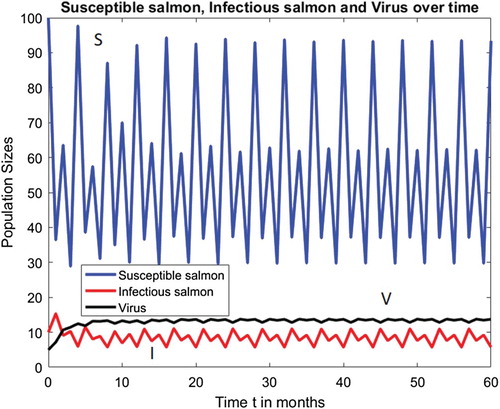
Figure shows ISAv disease induced period-doubling bifurcations route to chaos in the infectious salmon population, where the disease-free susceptible salmon population is on a locally asymptotically stable period 2 cycle. For example, when and all the other parameters are kept fixed at their current values in Figure , then
and Figure shows that Model (Equation7
(7)
(7) ) has a locally asymptotically stable endemic period 4 population cycle at
where the period of the disease-free susceptible salmon population cycle is 2. That is, unlike in Model (Equation7
(7)
(7) ), in Model (Equation20
(20)
(20) ) the equation for the total salmon population,
, is different from the disease-free equation, and the period of the disease-free susceptible salmon population cycle does not determine the period of the infectious salmon population cycle when
.
Figure 5. Bifurcation diagram for ISAv Model (Equation20(20)
(20) ): As
increases from values less than 1 to values greater than 1, the model dynamics changes from disease extinction to disease persistence on a periodic or chaotic population cycle.
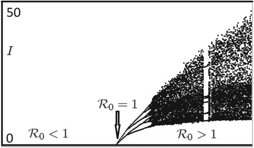
Figure 6. Model (Equation20(20)
(20) ) with
has a locally asymptotically stable period 4 population cycle when
and all the other parameter values are kept fixed at their current values in Figure .
5. Concluding remarks
Populations do not grow indefinitely over time, and density dependence or other factors tend to drive populations toward their carrying capacity. However, it is possible for real populations to experience some population fluctuations around the carrying capacity. These fluctuations can be periodic (cyclic) or erratic (chaotic). In this paper, we use a general autonomous discrete-time infectious disease model to extend the next generation matrix approach for calculating the basic reproduction number, , to account for populations with cyclic demographic dynamics. When
and the demographic equation (in the absence of the disease) has a locally asymptotically stable period k population cycle, we prove the local asymptotic stability of the disease-free period k cycle where
. That is, the disease dies out whenever
. Also, under the same period k demographic assumption, we prove that the disease-free period k population cycle is unstable and the disease persists when
(Theorem 2.1). An extension of the next generation matrix approach for calculating the basic reproduction number,
, to account for populations with chaotic and non-periodic demographic dynamics is an open problem.
We apply our theoretical results to discrete-time infectious disease models with a Ricker recruitment function that are formulated for SIR infections with and without vaccination, and ISAv infections in a salmon population. When , in the SIR model, the period of the disease-free S-cycle is numerically shown to be the same as the period of the I-cycle. That is, the demographic dynamics drives the SIR disease dynamics (see Figure ). However, we illustrate, in Figure , that the demographic dynamics does not drive the ISAv disease dynamics. Questions on establishing the possible connections between ISAv disease infections and observed population cycles in some salmon populations are open.
Acknowledgments
We thank the referees for their useful comments and suggestions. Preliminary ideas for this research were discussed during ICMA-VI Conference at University of Arizona in Tucson.
Disclosure statement
No potential conflict of interest was reported by the authors.
Additional information
Funding
References
- L. J. S. Allen, Some discrete-time SI, SIR and SIS epidemic models. Math. Biosc. 124 (1994), pp. 83–105. doi: 10.1016/0025-5564(94)90025-6
- L. J. S. Allen, P. van den Driessche, The basic reproduction number in some discrete-time epidemic models. J. Diff. Eqns. & Appl. 14(10–11) (2008), pp. 1127–1147. doi: 10.1080/10236190802332308
- N. Bacaër and E.H. Ait Dads, On the biological interpretation of a definition for the parameter R0 in periodic models, J. Math. Biol. 65 (2012), pp. 601–621. doi: 10.1007/s00285-011-0479-4
- J.T. Barton, An Introduction to Discrete Mathematical Modeling with Microsoft Office Excel, John Wiley & Sons, Inc, Hoboken, NJ, 2016.
- F. Brauer, Z. Feng, and C. Castillo-Chavez, Discrete epidemic models, Math. Biosc. Eng. 7(1) (2010), pp. 1–15. doi: 10.3934/mbe.2010.7.1
- C. Castillo-Chavez and A.-A. Yakubu, Dispersal, disease and life-history evolution, Math. Biosc. 173 (2001), pp. 35–53. doi: 10.1016/S0025-5564(01)00065-7
- J.M. Cushing and O. Diekmann, The many guises of R0 (a diadactic note), J. Theor. Biol. 404 (2016), pp. 295–302. doi: 10.1016/j.jtbi.2016.06.017
- J.M. Cushing and Z. Yicang, The net reproductive value and stability in matrix population models, Nat. Resour. Model. 8 (1994), pp. 297–333. doi: 10.1111/j.1939-7445.1994.tb00188.x
- M. Devold, B. Krossay, V. Aspehaug, and A. Nylund, Use of RT-PCR for diagnosis of infectious salmon anaemia virus (ISAv) in carrier sea trout Salmo trutta after experimental infection, Dis. Aquat. Org. 40 (2000), pp. 9–18. doi: 10.3354/dao040009
- O. Diekmann, J.A.P. Heesterbeek, and J.A.J. Metz, On the definition and computation of the basic reproduction ratio R0 in models for infectious diseases in heterogeneous populations, J. Math. Biol. 28 (1990), pp. 365–382. doi: 10.1007/BF00178324
- S. Elaydi, Discrete Chaos, Chapman & Hall/CRC, Boca Raton, FL, 2000.
- S. Elaydi and A.-A. Yakubu, Global stability of cycles: Lotka-Volterra competition model with stocking, J. Difference Equ. Appl. 8(6) (2002), pp. 537–549. doi: 10.1080/10236190290027666
- K. Falk, E. Namork, E. Rimstad, S. Mjaaland, and B.H. Dannevig, Characterization of infectious salmon anemia virus, an orthomyxo-like virus isolated from Atlantic salmon (Sahmo salar L.), J. Virol. 71 (1997), pp. 9016–9023.
- P.J. Hudson, A.P. Dobson, and D. Newborn, Prevention of population cycles by parasite removal, Science 282(5397) (1998), pp. 2256–2258. doi: 10.1126/science.282.5397.2256
- F.S.B. Kibenge, O.N. Garate, G.R. Johnson, R. Arriagada, M.J.T. Kibenge, and D. Wadowska, Isolation and identification of infectious salmon anaemia virus (ISAv) from Coho salmon in Chile, Dis. Aquat. Org. 45(1) (2001), pp. 9–18. doi: 10.3354/dao045009
- M. Krkosek, M.A. Lewis, and J.P. Volpe, Transmission dynamics of parasitic sea lice from farm to wild salmon, Proc. R. Soc. B. 272 (2005), pp. 689–696. doi: 10.1098/rspb.2004.3027
- D.A. Levy and C.C. Wood, Review of proposed mechanisms for sockeye salmon population cycles in the Fraser river, Bull. Math. Biol. 54(2–3) (1992), pp. 241–261. doi: 10.1007/BF02464832
- C.-K. Li and H. Schneider, Applications of Perron-Frobenius theory to population dynamics, J. Math. Biol. 44 (2002), pp. 450–462. doi: 10.1007/s002850100132
- M. Martcheva, An introduction to mathematical epidemiology, Springer Texts in Applied Mathematics 61, Springer, New York, 2015.
- R.M. May, Simple mathematical models with very complicated dynamics, Nature 261 (1976), pp. 459–467. doi: 10.1038/261459a0
- E. Milliken and S.S. Pilyugim, A model of infectious salmon anemia virus with viral diffusion between wild and farmed patches, Discrete & Cont. Dyn. Sys. B 21(6) (2016), pp. 1869–1893. doi: 10.3934/dcdsb.2016027
- W.E. Ricker, Stock and recruitment, J. Fish. Res. Board Can. 11 (1954), pp. 559–623. doi: 10.1139/f54-039
- A.R.E. Sinclair, D. Chitty, C.I. Stefan, and C.J. Krebs, Mammal population cycles: Evidence for intrinsic differences during snowshoe hare cycles, Can. J. Zool. 81(2) (2003), pp. 216–220. doi: 10.1139/z03-006
- J.H. Tien and D.J.D. Earn, Multiple transmission pathways and disease dynamics in a water borne pathogen model, Bull. Math. Biol. 72(6) (2010), pp. 1506–1533. doi: 10.1007/s11538-010-9507-6
- P. van den Driessche, Reproduction numbers of infectious disease models. Infect. Dis. Model. 2 (2017), pp. 1–16.
- P. van den Driessche and A.-A. Yakubu, Disease extinction versus persistence in discrete-time epidemic models, Bull. Math. Biol. 2018 (In press).
- S. Vike, S. Nylund, and A. Nylund, ISA virus in Chile. Evidence of vertical transmission, Arch. Virol. 154 (2009), pp. 1–8. doi: 10.1007/s00705-008-0251-2
- H.I. Wergeland, and R.A. Jakobsen, A salmonid cell line (TO) for production of infectious salmon anaemia virus (ISAv), Dis. Aquat. Org. 44 (2001), pp. 183–190. doi: 10.3354/dao044183
- A.-A. Yakubu, Introduction to discrete-time epidemic models, DIMACS Series in Discrete Math. Theor. Comput. Sci. 75 (2010), pp. 83–109. doi: 10.1090/dimacs/075/04