Stochastic two-group models with transmission dependent on host infectivity or susceptibility

ABSTRACT

Stochastic epidemic models with two groups are formulated and applied to emerging and re-emerging infectious diseases. In recent emerging diseases, disease spread has been attributed to superspreaders, highly infectious individuals that infect a large number of susceptible individuals. In some re-emerging infectious diseases, disease spread is attributed to waning immunity in susceptible hosts. We apply a continuous-time Markov chain (CTMC) model to study disease emergence or re-emergence from different groups, where the transmission rates depend on either the infectious host or the susceptible host. Multitype branching processes approximate the dynamics of the CTMC model near the disease-free equilibrium and are used to estimate the probability of a minor or a major epidemic. It is shown that the probability of a major epidemic is greater if initiated by an individual from the superspreader group or by an individual from the highly susceptible group. The models are applied to Severe Acute Respiratory Syndrome and measles.

KEYWORDS:

• Branching process
• Markov chain
• superspreader

MSC:

• 90D30
• 60J28

1. Introduction

In the twenty-first century, one of the biggest threats to public health is the spread of infectious diseases [35]. According to the World Health Organization, population mobility and the interconnectedness of the world's population have contributed to the global spread of infectious diseases [31,35]. Infectious diseases are one of the leading causes of death globally and the third leading cause of death in the United States [30]. Emerging and re-emerging infectious diseases include Severe Acute Respiratory Syndrome (SARS), Middle East Respiratory Syndrome (MERS), Ebola, Zika, influenza A, yellow fever, cholera, measles, pertussis, tuberculosis, and AIDS [35].

Recent emerging diseases have been attributed to highly infectious individuals, called superspreaders, who spread the disease to a large number of people [25]. Historically, superspreading events came to the forefront at the beginning of twentieth century. In the early 1900s, an individual referred to as Typhoid Mary was identified as a superspreader; she infected 51 people before being recognized as the source of infection [23]. Superspreading events have been identified in disease outbreaks of SARS, MERS, and Ebola [40]. Superspreading events are due to many reasons including physiological, immunological, and behavioural differences in individuals or due to emergence of a new pathogen or exposure to a new environment [34]. During the SARS outbreak in China in 2003, a total of 774 people died and 8096 were infected [40]. The index case, a superspreader, was responsible for infecting 125 people. During the MERS outbreak in 2015 in South Korea, 186 people were infected, and 36 people died [40]. Two superspreaders were responsible for infecting 106 people [40].

The waning of vaccine effectiveness or loss of protection from prior infection also cause some re-emerging diseases. Individuals may be highly susceptible to infection due to waning immunity. For example, in pertussis the immunity from vaccination remains effective for 4–12 years, whereas immunity from prior infection is much longer, 4–20 years [32,38]. For measles, the immunity from vaccination can protect against re-infection for up to 20 years for two doses but is less effective for only one dose [22]. In a measles outbreak in 2011, 110 high school students were infected; the attack rate was much less for students with two vaccine doses [11].

Modelling superspreaders has been the subject of many recent papers (e.g. [9,13,20,24–27]). Chowell et al. [9] modelled superspreaders in an MERS epidemic by considering a complex SEIR model with hospitalization, where specific superspreaders were modelled. In [24], Lee et al. extended the model for an MERS epidemic in South Korea with an SEIJR model, where J represented infectious individuals that were isolated. In a mathematical model for SARS with superspreaders, Mkhatshwa and Mummert [27] included four different classes in their model, susceptible, infected, superspreader, and recovered classes. In a two-group model applied to spread of SARS [26], transmission between patients in a hospital and outside visitors were analysed in terms of the final epidemic size. These preceding models were ordinary differential equations (ODEs). In the papers by James et al. [20] and Lloyd-Smith et al. [25], discrete-time branching processes were employed to relate transmission heterogeneity to superspreading events and to fit models to particular outbreaks. Lloyd-Smith et al. [25] showed for a heterogeneous population that average quantities such as the basic reproduction number do not adequately describe the effect of individual variation. Edholm et al. [13] developed a continuous-time Markov chain (CTMC) two-group model for superspreaders and non-superspreaders. They applied their stochastic model to MERS and Ebola, performed extensive numerical simulations, and used branching process approximations to compare disease epidemics initiated by superspreaders to non-superspreaders.

Similar to the model of Edholm et al. [13], we apply stochastic two-group models, CTMC models, and branching process approximations. We extend the two-group setting to consider the case where the transmission rate is dependent on either infectious or susceptible hosts, applicable to emerging and re-emerging infectious diseases. In addition, we prove there is a difference in probability of a minor or major epidemic, that is dependent on the particular group. It is verified that the probability of a major epidemic is greater if initiated by an infected individual from the highly infectious group (superspreader) or if initiated by an infected individual from the highly susceptible group. We discuss applications to SARS and measles.

In the next section, a two-group SIR model for epidemic spread is described, a system of ODEs. This model serves as a framework for formulation of two stochastic generalizations, CTMC models that include groups with either high and low infectivity or high and low susceptibility. In Section 4, continuous-time multitype branching processes are used to approximate the probability of a minor or a major epidemic. In Section 5, we show that the results extend to SEIR models when the group sizes are constant. We apply these models to potential SARS [26] and measles epidemics [11]. The sensitivity of ${\mathcal{R}}_0$ and the probability estimates to group size and transmission and recovery rates are also investigated.

2. Two-group SIR model

Consider a SIR model for a heterogeneous population with two groups. The model has two susceptible, two infectious and two recovered groups with different transmission and recovery rates for each group. The model has the following form: (1) $\begin{array}{rl}\frac{\mathrm{d}{S}_k}{\mathrm{d}t}& =-\frac{S_k}{N}\sum _{j=1}^2{\beta }_{kj}{I}_j,\\ \frac{\mathrm{d}{I}_k}{\mathrm{d}t}& =\frac{S_k}{N}\sum _{j=1}^2{\beta }_{kj}{I}_j-{\gamma }_k{I}_k,\\ \frac{\mathrm{d}{R}_k}{\mathrm{d}t}& ={\gamma }_k{I}_k,\end{array}$(1) for k=1, 2. The transmission rate from an infected individual in group j to a susceptible individual in group k is ${\beta }_{kj}>0$ and the recovery rate of an infected individual in group k is ${\gamma }_k>0$. The total population size $N=\sum _{k=1}^2{N}_k=\sum _{k=1}^2\left(S_k\right(t)+I_k(t)+R_k(t\left)\right)$ is constant and each group size $N_k$ is constant. The initial conditions are non-negative, $S_k\left(0\right)>0$, $I_k\left(0\right)\ge 0$, $\sum _k{I}_k\left(0\right)>0$ and $R_k\left(0\right)=0$ for k=1, 2. For simplicity, we let $R\left(t\right)=\sum _{k=1}^2{R}_k\left(t\right)$ denote all recovered individuals.

Two specific models are considered that distinguish between transmission dependent on the infectivity or the susceptibility of the host population. They are referred to as Model 1 and Model 2, respectively. In Model 1, the spread of disease is a result of high infectivity of the host, as in emerging diseases, such as MERS or SARS, where the presence of superspreaders may result in a large outbreak [8,33]. In Model 2, disease spread is a result of the lack of immunity in the host population from an infectious disease that may have either previously circulated in the population, as in re-emerging diseases, such as measles or pertussis [11,38].

For the two models, we assume that the transmission rate is separable ${\beta }_{kj}={\alpha }_k{\lambda }_j$ [36]. Either transmission depends primarily on the infectivity of the host, ${\alpha }_k{\lambda }_j={\beta }_j^I$ or the susceptibility of the host ${\alpha }_k{\lambda }_j={\beta }_k^S.$ The basic reproduction number ${\mathcal{R}}_0$, the average number of secondary infections generated by one infected individual, is computed using the next generation approach [12,19,36]. The basic reproduction number is (2) ${\mathcal{R}}_0=\sum _{i=1}^2\frac{{\beta }_i^m}{{\gamma }_i}\frac{N_i}{N}$(2) for m=I, S.

2.1. Model 1

In Model 1, the population is divided into two groups, where each group is defined by the ability to transmit the infection. The two groups are referred to as non-superspreaders and superspreaders. Superspreaders have been identified in diseases such as SARS, MERS, and Ebola [40]. Group 1 represents non-superspreaders, where $S_1$ and $I_1$ denote susceptible and infected non-superspreaders and in group 2, $S_2$ and $I_2$ denote susceptible and infected superspreaders. Individuals remain superspreaders or non-superspreaders during the course of the epidemic. Susceptible individuals $S_1$ infected by an individual from group $I_1$ or $I_2$ become infected non-superspreaders ($I_1$) and susceptible individuals $S_2$ infected by $I_1$ or $I_2$ become infected superspreaders ($I_2$). Therefore, the transmission rates depend on the infective group, ${\beta }_1^I$ or ${\beta }_2^I$. 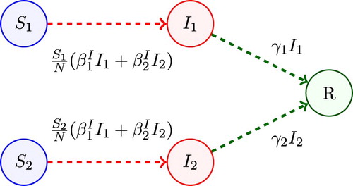A compartmental diagram for Model 1 is given in Figure 1. The basic reproduction number for Model 1 follows from Equation (2(2) ${\mathcal{R}}_0=\sum _{i=1}^2\frac{{\beta }_i^m}{{\gamma }_i}\frac{N_i}{N}$(2) ). That is, (3) ${\mathcal{R}}_0=\frac{{\beta }_1^I}{{\gamma }_1}\frac{N_1}{N}+\frac{{\beta }_2^I}{{\gamma }_2}\frac{N_2}{N}.$(3) In the special case that all individuals are either non-superspreaders or superspreaders ($S_1+I_1+R_1=N$ or $S_2+I_2+R_2=N$), the basic reproduction number simplifies to either ${\mathcal{R}}_0={\beta }_1^I/{\gamma }_1$ or ${\mathcal{R}}_0={\beta }_2^I/{\gamma }_2$, respectively.

Figure 1. Compartmental diagram for Model 1.

2.2. Model 2

Model 2 is applicable to re-emerging diseases, such as measles or pertussis. The population is divided into two groups, dependent on the susceptibility to infection. One group of individuals has immunity to the disease due to vaccination or to a prior infection of the disease referred to as the low-susceptible group (group 1) and a second group of individuals has little or no immunity as they have either not been vaccinated or the vaccine has waned over time. Group 2 is referred to as the high-susceptible group.

Variabies $S_1$ and $I_1$ represent the number of susceptible and infected individuals from the low-susceptible group 1 and $S_2$ and $I_2$ are the number of susceptible and infected individuals from the high-susceptible group 2. Individuals from $S_1$ after being infected by either $I_1$ or $I_2$ become $I_1$ and individuals from $S_2$ after being infected by either $I_1$ or $I_2$ become $I_2$. The transmission parameters depend on host susceptibility for each group, ${\beta }_1^S$ or ${\beta }_2^S$. 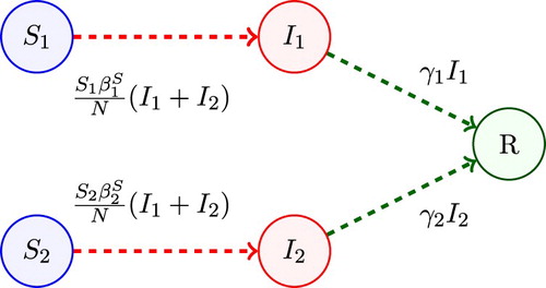A compartmental diagram of Model 2 is given in Figure 2. The basic reproduction number is (4) ${\mathcal{R}}_0=\frac{{\beta }_1^S}{{\gamma }_1}\frac{N_1}{N}+\frac{{\beta }_2^S}{{\gamma }_2}\frac{N_2}{N}.$(4) If there is a single group, either low-susceptible or high-susceptible, ($S_1+I_1+R_1=N$ or $S_2+I_2+R_2=N$), then the basic reproduction numbers simplify to ${\mathcal{R}}_0={\beta }_1^S/{\gamma }_1$ or ${\mathcal{R}}_0={\beta }_2^S/{\gamma }_2$, respectively.

Figure 2. Compartmental diagram for Model 2.

3. CTMC models

We formulate a stochastic CTMC model with discrete random variables for the number of individuals. Stochastic variability may lead to a minor epidemic with a few individuals infected instead of a full scale epidemic with many individuals infected. For simplicity, the same notation for the variables is used for the CTMC model as for the ODE model. That is, $S_k\left(t\right),I_k\left(t\right),R_k\left(t\right)\in \{0,1,\dots ,N_k\},k=1,2,$ with $t\in [0,\mathrm{\infty })$ and $R\left(t\right)=R_1\left(t\right)+R_2\left(t\right)$. Let $\mathrm{\Delta }{S}_k\left(t\right)=S_k(t+\mathrm{\Delta }t)-S_k\left(t\right),$ $\mathrm{\Delta }{I}_k\left(t\right)=I_k(t+\mathrm{\Delta }t)-I_k\left(t\right)$, and $\mathrm{\Delta }R\left(t\right)=R(t+\mathrm{\Delta }t)-R\left(t\right)$ for k=1, 2. The values of these random variables are denoted by lower case variables, $s_k,i_k,$ and r.

3.1. Model 1

The infinitesimal transition probabilities define the CTMC Model 1, e.g. [1,21]. For example, the transition from a susceptible to an infectious individual for the non-superspreader group is defined as follows: $\begin{array}{rl}& \mathbb{P}\left(\right(\mathrm{\Delta }{S}_1,\mathrm{\Delta }{I}_1,\mathrm{\Delta }{S}_2,\mathrm{\Delta }{I}_2,\mathrm{\Delta }R\left)\right(t)=(-1,1,0,0,0\left)|\right(S_1,I_1,S_2,I_2,R\left)\right(t)=(s_1,i_1,s_2,i_2,r\left)\right)\\ & ={\beta }_1^I{i}_1\frac{s_1}{N}\mathrm{\Delta }t+{\beta }_2^I{i}_2\frac{s_1}{N}\mathrm{\Delta }t+o\left(\mathrm{\Delta }t\right).\end{array}$ A list of the four events corresponding to either infection or recovery is given in Table 1.

Table 1. Infinitesimal transition probabilities for Model 1.

Event	$(\mathrm{\Delta }{S}_1,\mathrm{\Delta }{I}_1,\mathrm{\Delta }{S}_2,\mathrm{\Delta }{I}_2,\mathrm{\Delta }R)$	Probability
$S_1\to I_1$	$(-1,1,0,0,0)$	$({\beta }_1^I{i}_1+{\beta }_2^I{i}_2)\frac{s_1}{N}\mathrm{\Delta }t+o\left(\mathrm{\Delta }t\right)$
$S_2\to I_2$	$(0,0,-1,1,0)$	$({\beta }_1^I{i}_1+{\beta }_2^I{i}_2)\frac{s_2}{N}\mathrm{\Delta }t+o\left(\mathrm{\Delta }t\right)$
$I_1\to R$	$(0,-1,0,0,1)$	${\gamma }_1{i}_1\mathrm{\Delta }t+o\left(\mathrm{\Delta }t\right)$
$I_2\to R$	$(0,0,0,-1,1)$	${\gamma }_2{i}_2\mathrm{\Delta }t+o\left(\mathrm{\Delta }t\right)$

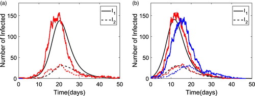
The solution dynamics for Model 1 are illustrated for the two infectious classes in Figure 3 for the ODE and CTMC Model 1 when ${\mathcal{R}}_0=2.86$ with population size N=1000 and the highly infectious group size $N_2=100$. The group reproduction numbers are ${\beta }_1^I/{\gamma }_1=0.4$ and ${\beta }_2^I/{\gamma }_2=25$. In Figure 3(a), an epidemic is initiated by a non-superspreader, $I_1\left(0\right)=1$ and $I_2\left(0\right)=0$, whereas in Figure 3(b), the epidemic is initiated with a superspreader, $I_1\left(0\right)=0$ and $I_2\left(0\right)=1$. 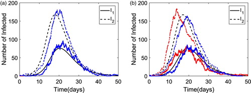The ODE solution and two sample paths of the CTMC model are plotted in each figure. For the two sample paths in Figure 3(a), only one sample path yields a major epidemic, while the other path yields a minor epidemic with a few infectious cases. However, in Figure 3(b), both sample paths yield a major epidemic. It is notable that an epidemic occurs earlier when initiated with a superspreader than with a non-superspreader [13].

Figure 3. Numerical solution of the ODE model and two sample paths of the CTMC for Model 1 with parameter values ${\beta }_1^I=0.2,$ ${\beta }_2^I=5$, ${\gamma }_1=0.5$, ${\gamma }_2=0.2$, $N=1000,$ and $N_2=100$ (${\mathcal{R}}_0=2.86$). The number of non-superspreaders is plotted with a solid curve whereas superspreaders are plotted with a dashed curve. In (a), $I_1\left(0\right)=1$ and $I_2\left(0\right)=0$, only one sample path illustrates a major epidemic and in (b), $I_1\left(0\right)=0$ and $I_2\left(0\right)=1$, both sample paths illustrate a major epidemic. (a) $I_1\left(0\right)=1,I_2$(0)=0. (b) $I_1\left(0\right)=0,I_2$(0)=1.

3.2. Model 2

The CTMC for Model 2 can be defined in a similar way as in Model 1 with the exception that the transmission rates depend on host susceptibility. The infinitesimal transition probabilities are given in Table 2.

Table 2. Infinitesimal transition probabilities for Model 2.

Event	$(\mathrm{\Delta }{S}_1,\mathrm{\Delta }{I}_1,\mathrm{\Delta }{S}_2,\mathrm{\Delta }{I}_2,\mathrm{\Delta }R)$	Probability
$S_1\to I_1$	$(-1,1,0,0,0)$	${\beta }_1^S\frac{s_1}{N}(i_1+i_2)\mathrm{\Delta }t+o\left(\mathrm{\Delta }t\right)$
$S_2\to I_2$	$(0,0,-1,1,0)$	${\beta }_2^S\frac{s_2}{N}(i_1+i_2)\mathrm{\Delta }t+o\left(\mathrm{\Delta }t\right)$
$I_1\to R$	$(0,-1,0,0,1)$	${\gamma }_1{i}_1\mathrm{\Delta }t+o\left(\mathrm{\Delta }t\right)$
$I_2\to R$	$(0,0,0,-1,1)$	${\gamma }_2{i}_2\mathrm{\Delta }t+o\left(\mathrm{\Delta }t\right)$

An example of the solution dynamics of the infectious classes are plotted for Model 2 in Figure 4 when ${\mathcal{R}}_0=2.86$. The same parameter values are applied as in Figure 3, except the population size is N=5000 with high-susceptible group size $N_2=500$. Two sample paths of the CTMC Model 2 are graphed with the ODE solution. To obtain an outbreak size similar to that in Model 1 (Figure 3), a larger population size is assumed.

Figure 4. Numerical solution of the ODE model and two sample paths of the CTMC for Model 2 with parameter values ${\beta }_1^S=0.2$, ${\beta }_2^S=5,$ ${\gamma }_1=0.5,$ ${\gamma }_2=0.2,$ $N=5000,$ and $N_2=500$ (${\mathcal{R}}_0=2.86$). The number of infectious individuals from the low-susceptible group is plotted with a solid curve whereas the number of infectious individuals from the high-susceptible group is plotted with a dashed curve. In (a), $I_1\left(0\right)=1$ and $I_2\left(0\right)=0$, only one sample path illustrates a major epidemic and in (b), $I_1\left(0\right)=0$ and $I_2\left(0\right)=1$, both sample paths illustrate a major epidemic. (a) $I_1\left(0\right)=1,I_2$(0)=0. (b) $I_1\left(0\right)=0,I_2$(0)=1.

4. Multitype branching process approximation

The CTMC model is approximated by a Galton–Watson multitype branching process (BP) near the disease-free equilibrium (DFE) [5,18]. In the BP approximation, it is assumed that the population is at the DFE and a small number of infectious individuals is introduced into the population. The goal is to use the BP approximation to estimate the probability of a minor or a major epidemic. The probabilities for an infection or a recovery are defined for an infectious individual in each group, through a generating function. The transmission dynamics for infectious individuals within each group $I_1$ and $I_2$ act like a multitype birth and death process, where a birth is a new infection and death is a recovery. The probability of a minor epidemic in the CTMC model corresponds to the probability of ultimate extinction (as $t\to \mathrm{\infty }$) in the birth and death process. It is verified in Appendix 1 from the backward Kolmogorov equations and from the assumption about independence of $I_1$ and $I_2$ that for a small number of infectious individuals, the probability of ultimate extinction is the minimal fixed point of the offspring probability generating functions (pgfs). An offspring pgf for $I_1$ has the general form $f_1(u_1,u_2)=\sum _{l=0}^{\mathrm{\infty }}\sum _{m=0}^{\mathrm{\infty }}{\mathbb{P}}_1(\ell ,m)u_1^{\ell }{u}_2^m,$ where $P_1(\ell ,m)$ is the probability there are ℓ infectious individuals of type $I_1$ and m of type $I_2$ generated from one infectious individual of type 1 given $I_1\left(0\right)=1$ and $I_2\left(0\right)=0$. A similar definition applies to $I_2$, given $I_1\left(0\right)=0$ and $I_2\left(0\right)=1$. A fixed point $(q_1,q_2)$ of the pgfs, $f_j(q_1,q_2)=q_j$, j=1, 2 lies in $[0,1]\times [0,1]$. The independent assumption in the BP approximation and the differential equations derived from the Kolmogorov equations yield estimates for the probability of ultimate extinction. Applying this estimate to the CTMC model, it can be interpreted as the probability of a minor epidemic, given $I_1\left(0\right)=i_1$ and $I_2\left(0\right)=i_2$, ${\mathbb{P}}_{\mathrm{minor}}=q_1^{i_1}{q}_2^{i_2},$ where ($q_1,q_2)$ is the minimal fixed point in $[0,1]\times [0,1]$, e.g. [3–5,18,39]. In addition, the probability of a major epidemic in the CTMC model is approximately ${\mathbb{P}}_{\mathrm{major}}=1-{\mathbb{P}}_{\mathrm{minor}}.$

4.1. Model 1

The BP approximation of the CTMC model near the DFE is a linear approximation of the rates, $S_1=N_1$ and $S_2=N_2.$ These rates are defined in Table 3.

Table 3. Branching process approximation for Model 1.

($\mathrm{\Delta }{I}_1,\mathrm{\Delta }{I}_2$)	Probability
(1,0)	$({\beta }_1^I{i}_1+{\beta }_2^I{i}_2)\frac{N_1}{N}\mathrm{\Delta }t+o\left(\mathrm{\Delta }t\right)$
(0,1)	$({\beta }_1^I{i}_1+{\beta }_2^I{i}_2)\frac{N_2}{N}\mathrm{\Delta }t+o\left(\mathrm{\Delta }t\right)$
$(-1,0)$	${\gamma }_1{i}_1\mathrm{\Delta }t+o\left(\mathrm{\Delta }t\right)$
$(0,-1)$	${\gamma }_2{i}_2\mathrm{\Delta }t+o\left(\mathrm{\Delta }t\right)$

For Model 1, the offspring pgf for non-superspreaders, given $I_1\left(0\right)=1$ and $I_2\left(0\right)=0$, is (5) $f_1(u_1,u_2)=\frac{{\gamma }_1+{\beta }_1^I\frac{N_1}{N}{u}_1^2+{\beta }_1^I\frac{N_2}{N}{u}_1{u}_2}{{\gamma }_1+{\beta }_1^I},$(5) $u_k\in [0,1],$ k=1,2. The term ${\gamma }_1/({\gamma }_1+{\beta }_1^I)$ is the probability of recovery of a non-superspreader, ${\beta }_1^I\left(N_1/N\right)/({\gamma }_1+{\beta }_1^I)$ is the probability of infecting another non-superspreader and ${\beta }_2^I\left(N_2/N\right)/({\gamma }_1+{\beta }_1^I)$ is probability of infecting a superspreader. The offspring pgf for superspreaders, given $I_1\left(0\right)=0$ and $I_2\left(0\right)=1$, is (6) $f_2(u_1,u_2)=\frac{{\gamma }_2+{\beta }_2^I\frac{N_2}{N}{u}_2^2+{\beta }_2^I\frac{N_1}{N}{u}_1{u}_2}{{\gamma }_2+{\beta }_2^I},$(6) $u_k\in [0,1]$, k=1,2. The term ${\gamma }_2/({\gamma }_2+{\beta }_2^I)$ is the probability of recovery of a superspreader, ${\beta }_2^I\left(N_2/N\right)/({\gamma }_2+{\beta }_2^I)$ is the probability of infecting another superspreader, and ${\beta }_2^I\left(N_1/N\right)/({\gamma }_2+{\beta }_2^I)$ is the probability of infecting a non-superspreader [3].

Application of multitype BP theory, Equations (5(5) $f_1(u_1,u_2)=\frac{{\gamma }_1+{\beta }_1^I\frac{N_1}{N}{u}_1^2+{\beta }_1^I\frac{N_2}{N}{u}_1{u}_2}{{\gamma }_1+{\beta }_1^I},$(5) ) and (6(6) $f_2(u_1,u_2)=\frac{{\gamma }_2+{\beta }_2^I\frac{N_2}{N}{u}_2^2+{\beta }_2^I\frac{N_1}{N}{u}_1{u}_2}{{\gamma }_2+{\beta }_2^I},$(6) ) and the backward Kolmogorov differential equations lead to an ODE for probability of disease extinction at time t [3,5,18]. The steady-state solutions of this equation are the fixed points of pgfs (5(5) $f_1(u_1,u_2)=\frac{{\gamma }_1+{\beta }_1^I\frac{N_1}{N}{u}_1^2+{\beta }_1^I\frac{N_2}{N}{u}_1{u}_2}{{\gamma }_1+{\beta }_1^I},$(5) ) and (6(6) $f_2(u_1,u_2)=\frac{{\gamma }_2+{\beta }_2^I\frac{N_2}{N}{u}_2^2+{\beta }_2^I\frac{N_1}{N}{u}_1{u}_2}{{\gamma }_2+{\beta }_2^I},$(6) ) (probability of ultimate extinction). When ${\mathcal{R}}_0>1$, there are at least two steady-states, one with $(q_1,q_2)=(1,1)$ and at another one with $q_i<1$. The minimal fixed point is stable and this point yields the probability of ultimate extinction (or the probability of a minor epidemic in the CTMC model). When ${\mathcal{R}}_0\le 1$, there is only one fixed point, $q_i=1$, so that the probability of ultimate disease extinction is equal to one. Details of this derivation are given in Appendix 1.

In Figure 5, the dashed curves are probability of a minor epidemic when initiated by a non-superspreader $q_1$ or a superspreader $q_2$. The points marked by ‘x’ are estimates for the probability of a minor epidemic calculated from 10,000 sample paths of the CTMC model. A threshold of 20 is assumed to indicate an outbreak. The peak level of infection for both infected groups in the deterministic model reaches values greater than 20 for ${\mathcal{R}}_0>1.5$, therefore, this a reasonable assumption for numerical computations. In particular for each sample path, if $I_1+I_2\ge 20$, then it is considered a major epidemic, but if the total number infected hits zero before reaching 20, then it is classified as a minor epidemic. Figure 5 shows that the CTMC estimate of a minor epidemic (proportion hitting zero from 10,000 sample paths) agrees with the BP estimate.

Figure 5. Graphs of the probability of minor epidemic as a function of $N_2$ the number of superspreaders. The probability of a minor epidemic if it is initiated by a non-superspreader ($q_1)$ or a superspreader ($q_2)$ and the value of ${\mathcal{R}}_0$ are graphed for Model 1. Parameter values are ${\gamma }_1=0.5,$ ${\gamma }_2=0.2,$ ${\beta }_1^I=0.2,$ ${\beta }_2^I=5,$ and $N=1000,$ where the size of the superspreader population ranges from $N_2=1$ to 110. The BP analytical estimates of probability of a minor epidemic (dashed and dashed-dot curves) are compared to estimates computed from 10,000 sample paths of the CTMC model (marked by a ‘x’).

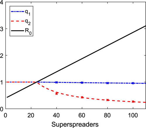
Figure 5 illustrates that the probability of a minor epidemic when initiated by a non-superspreader is greater than when initiated by a superspreader. We verify this result always holds true when ${\mathcal{R}}_0>1$ and ${\beta }_1^I/{\gamma }_1<{\beta }_2^I/{\gamma }_2$. The proof is relegated to Appendix 3.

Theorem 4.1

Assume that ${\mathcal{R}}_0>1$ and ${\beta }_1^I/{\gamma }_1<{\beta }_2^I/{\gamma }_2$ in the BP approximation for Model 1. Then the probability of a minor epidemic when initiated by a non-superspreader is greater than the probability of a minor epidemic when initiated by a superspreader, $q_1>q_2$. In addition, if ${\mathcal{R}}_0\le 1,$ then $q_1=1=q_2$. In the special case ${\beta }_1^I/{\gamma }_1={\beta }_2^I/{\gamma }_2,$ $q_1=1/{\mathcal{R}}_0=q_2$.

In the special case of a single group, the result of Theorem 4.1 simplifies to the classic result of Whittle [39]. Whittle verified for the classic SIR CTMC model, ${\mathbb{P}}_{\mathrm{minor}}=(1/{\mathcal{R}}_0{)}^i$, where $I\left(0\right)=i$.

4.2. Model 2

The transition rates for the BP approximation of the CTMC Model 2 near the DFE are given in Table 4.

Table 4. Branching process approximation for Model 2.

($\mathrm{\Delta }{I}_1,\mathrm{\Delta }{I}_2$)	Probability
(1,0)	${\beta }_1^S\frac{N_1}{N}(i_1+i_2)\mathrm{\Delta }t+o\left(\mathrm{\Delta }t\right)$
(0,1)	${\beta }_2^S\frac{N_2}{N}(i_1+i_2)\mathrm{\Delta }t+o\left(\mathrm{\Delta }t\right)$
$(-1,0)$	${\gamma }_1{i}_1\mathrm{\Delta }t+o\left(\mathrm{\Delta }t\right)$
$(0,-1)$	${\gamma }_2{i}_2\mathrm{\Delta }t+o\left(\mathrm{\Delta }t\right)$

The offspring pgf for an individual from the low-susceptible group ($I_1\left(0\right)=1,I_2\left(0\right)=0$) is given by (7) $f_1(u_1,u_2)=\frac{{\gamma }_1+{\beta }_1^S\frac{N_1}{N}{u}_1^2+{\beta }_2^S\frac{N_2}{N}{u}_1{u}_2}{{\gamma }_1+{\beta }_1^S\frac{N_1}{N}+{\beta }_2^S\frac{N_2}{N}},$(7) where ${\gamma }_1/({\gamma }_1+{\beta }_1^S(N_1/N)+{\beta }_2^S\left(N_2/N\right))$ is the probability of recovery, ${\beta }_1^S\left(N_1/N\right)/({\gamma }_1+{\beta }_1^S(N_1/N)+{\beta }_2^S\left(N_2/N\right))$ is the probability of infecting an $S_1$ individual and ${\beta }_2^S\left(N_2/N\right)/({\gamma }_1+{\beta }_1^S(N_1/N)+{\beta }_2^S\left(N_2/N\right))$ is the probability of infecting an $S_2$ individual. The offspring pgf for an individual from the high-susceptible group ($I_1=0,I_2=1$) is given by (8) $f_2(u_1,u_2)=\frac{{\gamma }_2+{\beta }_2^S\frac{N_2}{N}{u}_2^2+{\beta }_1^S\frac{N_1}{N}{u}_1{u}_2}{{\gamma }_2+{\beta }_2^S\frac{N_2}{N}+{\beta }_1^S\frac{N_1}{N}},$(8) where ${\gamma }_2/({\gamma }_2+{\beta }_2^S(N_2/N)+{\beta }_1^S(N_1/N\left)\right)$ is the probability of recovery, ${\beta }_2^S\left(N_2/N\right)/({\gamma }_2^S+{\beta }_2^S(N_2/N)+{\beta }_1^S(N_1/N\left)\right)$ is the probability of infecting an $S_2$ individual, and ${\beta }_2^S\left(N_1/N\right)/({\gamma }_2+{\beta }_2^S(N_2/N)N+{\beta }_1^S(N_1/N\left)\right)$ is the probability of infecting an $S_1$ individual (see, e.g. [3]).

In Figure 6, the values of the probability of a minor epidemic $q_1$ and $q_2$ as estimated from the BP approximation are compared with a numerical estimate computed from 10,000 sample paths of the CTMC. Of these 10,000 sample paths, the proportion of sample paths such that $I_1+I_2$ hits zero before reaching a value of 20 is assumed to be an estimate of $q_1$ or $q_2$. (We choose 20 as a threshold, as the peak level of infection for both infected groups in the deterministic model is greater than 20).

Figure 6. Graphs of the probability of minor epidemic are graphed as a function of $N_2$, the high-susceptible group. The probability of a minor epidemic if initiated by an individual from the low-susceptible group ($q_1)$ or high susceptible group ($q_2)$ and the value of ${\mathcal{R}}_0$ are graphed for Model 2. Parameter values are ${\gamma }_1=0.5,$ ${\gamma }_2=0.2,$ ${\beta }_1^S=0.2,$ ${\beta }_2^S=5,$ and N=5000, where the size of the high-susceptible group ranges from $N_2=1$ to 600. The BP analytical estimates of probability of a minor epidemic (dashed and dashed-dot curves) are compared to estimates from 10,000 sample paths of the CTMC model (marked by a ‘x’).

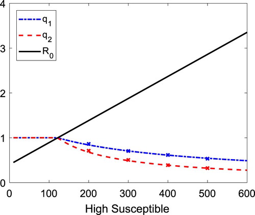
In the stochastic Model 2, it is the magnitude of the recovery rates rather than transmission rates that differentiates the probability estimates for a minor epidemic between the two groups. The proof of the following theorem is given in Appendix 4.

Theorem 4.2

Assume ${\mathcal{R}}_0>1$ and ${\gamma }_1>{\gamma }_2$ in the BP approximation of Model 2. Then the probability of a minor epidemic when initiated by an infected individual from the low-susceptible group is greater than when initiated by an infected individual from the high-susceptible group, $q_1>q_2$. In addition, if ${\mathcal{R}}_0\le 1$, then $q_1=1=q_2$. In the special case ${\gamma }_1={\gamma }_2$, $q_1=1/{\mathcal{R}}_0=q_2.$

5. SEIR two-group model with multiple latent stages

We show that the previous results for multitype BP extend to models with m latent or exposed stages, $E_{k,1},\dots ,E_{k,m}$, k=1, 2 for the case that the group sizes are constant. During a latent or exposed stage, individuals are infected but not yet infectious, meaning they do not spread the infection to others. Multiple exposed stages account for the delay prior to the infectious period. In particular, the ODE model for stages $S_k$ and $R_k$ is the same as in (1(1) $\begin{array}{rl}\frac{\mathrm{d}{S}_k}{\mathrm{d}t}& =-\frac{S_k}{N}\sum _{j=1}^2{\beta }_{kj}{I}_j,\\ \frac{\mathrm{d}{I}_k}{\mathrm{d}t}& =\frac{S_k}{N}\sum _{j=1}^2{\beta }_{kj}{I}_j-{\gamma }_k{I}_k,\\ \frac{\mathrm{d}{R}_k}{\mathrm{d}t}& ={\gamma }_k{I}_k,\end{array}$(1) ) but the other stages have the form: $\begin{array}{rl}\frac{\mathrm{d}{E}_{k,1}}{\mathrm{d}t}& =\frac{S_k}{N}\sum _{j=1}^2{\beta }_{kj}{I}_j-{\alpha }_{k,1}{E}_{k,1},\\ & ⋮\\ \frac{\mathrm{d}{E}_{k,m}}{\mathrm{d}t}& ={\alpha }_{k,m-1}{E}_{m-1,1}-{\alpha }_{k,m}{E}_{k,m},\\ \frac{\mathrm{d}{I}_k}{\mathrm{d}t}& ={\alpha }_{k,m}{E}_{k,m}-{\gamma }_k{I}_k,\end{array}$ where the new parameter ${\alpha }_{k,m}$ is the transition rate between the k and k+1 latent stage, $N\left(t\right)=\sum _{k=1}^2{N}_k=\sum _{k=1}^2\left(S_k\right(t)+\sum _{j=1}^m{E}_{k,j}(t)+I_k(t)+R_k(t\left)\right)$, with initial conditions $S_k\left(0\right)>0$, $E_k\left(0\right)\ge 0$, $I_k\left(0\right)>0$ and $R_k\left(0\right)=0$. New infections are due to the infectious stages $I_k$. We make the same assumptions regarding the transmission rates as in model (1(1) $\begin{array}{rl}\frac{\mathrm{d}{S}_k}{\mathrm{d}t}& =-\frac{S_k}{N}\sum _{j=1}^2{\beta }_{kj}{I}_j,\\ \frac{\mathrm{d}{I}_k}{\mathrm{d}t}& =\frac{S_k}{N}\sum _{j=1}^2{\beta }_{kj}{I}_j-{\gamma }_k{I}_k,\\ \frac{\mathrm{d}{R}_k}{\mathrm{d}t}& ={\gamma }_k{I}_k,\end{array}$(1) ), ${\beta }_{jk}={\beta }_j^I$ for Model 1 and ${\beta }_{jk}={\beta }_k^S$ for Model 2. Another important assumption is that there are no deaths. Each group size is constant. Applying the next generation matrix approach [36], it follows that ${\mathcal{R}}_0$ has the same expression as in Equation (2(2) ${\mathcal{R}}_0=\sum _{i=1}^2\frac{{\beta }_i^m}{{\gamma }_i}\frac{N_i}{N}$(2) ).

For the corresponding CTMC SEIR model, the infinitesimal transition rates for the latent stages are $\begin{array}{rl}\mathbb{P}\left(\right(\mathrm{\Delta }{E}_{k,j},\mathrm{\Delta }{E}_{k,j+1})=(-1,1\left)|E_{k,j}\right(t)=e_{k,j})& ={\alpha }_{k,j}{e}_{k,j}\mathrm{\Delta }t+o\left(\mathrm{\Delta }t\right),j=1,2\\ \mathbb{P}\left(\right(\mathrm{\Delta }{E}_{k,m},\mathrm{\Delta }{I}_k)=(-1,1\left)|E_{k,m}\right(t)=e_{k,m})& ={\alpha }_{k,m}{e}_{k,m}\mathrm{\Delta }t+o\left(\mathrm{\Delta }t\right).\end{array}$ In the BP approximation of the CTMC SEIR model with two groups and m latent stages, there are 2m+2 pgfs. However, as there are no deaths in any of the 2 m latent stages, given $E_{k,j}\left(0\right)=1$, it follows that the jth latent stage progresses to the next latent stage $E_{k,j+1}$ or to $I_k$ with probability one. It follows that the probability of disease extinction beginning from any latent stage $E_{k,j}$ is the same as the probability of disease extinction beginning from $I_k$ (Appendix 3). Therefore, Theorems 4.1 and 4.2 are applicable to the SEIR models with two groups.

In the next two sections, we apply Model 1 and 2 with one latent stage to hypothetical models of SARS and measles. The BP approximation is used to estimate the probability of a major epidemic and the estimate is compared to CTMC simulations.

6. Application to SARS

SARS, a recent emerging disease, was first identified in the early part of the twenty-first century. In 2003, an outbreak of SARS occurred in Singapore with a total 206 cases, as reported in [16]. Three superspreaders were identified who infected a total 76 individuals. The index case was a superspreader who was admitted to a hospital on March 1 and was isolated on March 6. By this time, the index case had infected 24 individuals. Two other superspreaders infected 25 and 27 individuals, respectively. Magal et al. [26] formulated an ODE two-group model with no latent stage, where the two groups are individuals inside and outside of a hospital setting. We use their model as motivation to formulate a hypothetical model for SARS, but applying the assumptions in Model 1 with a latent stage, a homogeneous mixing population, and two transmission rates for the infectious individuals, ${\beta }_i^I,i=1,2.$ We use some parameter values comparable to Magal et al. [26] for population sizes N=2500 and $N_2=300$ (Magal: N=2300 and $N_2=300$), ${\beta }_1^I=0.15$ (Magal: ${\beta }_{11}N=0.184$ outside of the hospital), and the recovery rate for group 1, ${\gamma }_1=0.8$ (Magal: ${\eta }_1=0.4$ outside of the hospital). We consider a range of values for ${\beta }_2^I$ and ${\gamma }_2$ (Table 6), where ${\beta }_2^I\ge {\beta }_1^I$ and ${\gamma }_2\le {\gamma }_1$. Generally, SARS patients are contagious when they exhibit symptoms [29]. The latent period reported by the Centers for Disease Control is 2–7 days [29]. Therefore, we assume the transition rate from $E_k$ to $I_k$ is ${\alpha }_k=1/5$ per day for groups k=1,2. Estimates for the basic reproduction number for SARS in Singapore include a range of 2.3 to 4 prior to a issuance of a global alert [37]. With control efforts in place for SARS, estimates for the basic reproduction number range from 0.49 to 2.47 [10]. We explore a wider range of ${\mathcal{R}}_0$ values in Table 6. A summary of the parameter values for our example of the two-group SEIR Model 1 for SARS is given in Table 5.

Table 5. Parameter values for SARS.

Parameters	N	$N_2$	${\beta }_1^I$	${\beta }_2^I$	${\gamma }_1$	${\gamma }_2$	${\alpha }_1$	${\alpha }_2$
Values	2500	300	0.15	varies	0.8	varies	0.2	0.2

Table 6. The BP approximation of a major epidemic (either $1-q_1$ or $1-q_2$) is compared to the CTMC simulations based on 10,000 sample paths.

${\beta }_2^I$	${\gamma }_2$	$I_1\left(0\right)$	$I_2\left(0\right)$	BP	CTMC	${\mathcal{R}}_0$	${\mathcal{S}}_{{\beta }_1^I}^{{\mathcal{R}}_0}$	${\mathcal{S}}_{{\beta }_2^I}^{{\mathcal{R}}_0}$
2	0.18	1	0	0.010	0.010	1.498	0.277	1.998
4	0.25	1	0	0.015	0.015	2.085	0.344	4.003
8	0.25	1	0	0.020	0.021	3.857	0.661	15.38
6	0.04	1	0	0.025	0.025	18.165	2.997	327.0
2	0.06	0	1	0.800	0.785	4.165	0.687	16.66
4	0.17	0	1	0.700	0.704	2.989	0.493	8.438
6	0.34	0	1	0.600	0.608	2.283	0.377	4.834
8	0.67	0	1	0.400	0.416	1.598	0.264	2.289

Notes: The sensitivity indices ${\mathcal{S}}_p^{{\mathcal{R}}_0}$ for ${\mathcal{R}}_0$ are reported for parameters $p={\beta }_1^I$ and $p={\beta }_2^I$. Parameter values are taken from Table 5.

The probabilities $1-q_1$ and $1-q_2$ of a major epidemic when the epidemic is initiated by one non-superspreader or by one superspreader, respectively, are graphed in Figure 7 as a function of the transmission rate ${\beta }_2^I$ and the recovery rate ${\gamma }_2$. In addition, the contours of this surface are graphed for fixed values of the probabilities. The surfaces and contours are computed from the BP approximation. It can be easily seen that $1-q_2\gg 1-q_1$. On each of the contours, a value is selected and compared with the value obtained from 10,000 sample paths of the CTMC model. The results are recorded in Table 6. The ‘x’ marks on the contours in Figure 7 are the estimates from the CTMC simulations. If a sample path reaches $I_1+I_2\ge 15$, the epidemic is assumed to be major. If the value of $I_1+I_2$ hits zero before reaching 15, it is assumed to be a minor epidemic. The proportion of sample paths out of 10,000, where the infected population reaches 15 or greater is the estimate for a major epidemic. There is good agreement between the BP approximation and the CTMC simulations, as shown in Table 6. Evident in the top two graphs in Figure 7, are the differences in the vertical scales. The probability of a major epidemic, initiated with an infected superspreader is significantly greater than if initiated with an infected non-superspreader. (The value of 15 is chosen as a threshold since the peak value of infected for both groups is greater than 15 in the deterministic models for the range of ${\mathcal{R}}_0$ values in Table 6.)

Figure 7. Probability of a major epidemic $1-q_1$ and $1-q_2$ are plotted as a function of the transmission ${\beta }_2^I$ and recovery ${\gamma }_2$ rates given one non-superspreader or one superspreader. Other parameter values for SARS are taken from Table 5. In addition, contours for each surface are graphed at the bottom of the figures, for several fixed probabilities.

As the values of $q_i$ depend on ${\mathcal{R}}_0$ (Theorem 4.1), we performed a sensitivity analysis of the basic reproduction number ${\mathcal{R}}_0$, given in Equation (3(3) ${\mathcal{R}}_0=\frac{{\beta }_1^I}{{\gamma }_1}\frac{N_1}{N}+\frac{{\beta }_2^I}{{\gamma }_2}\frac{N_2}{N}.$(3) ), with respect to parameters ${\beta }_i^I$, i=1, 2. Applying the method in [7], the normalized forward sensitivity index for ${\mathcal{R}}_0$ with respect to the parameter p equals ${\mathcal{S}}_p^{{\mathcal{R}}_0}=\frac{\mathrm{\partial }{\mathcal{R}}_0}{\mathrm{\partial }p}\cdot \frac{p}{{\mathcal{R}}_0}.$ The sensitivity indices only need to be determined for ${\beta }_i^I$, i=1,2, since the sensitivity with respect to the other parameters ${\gamma }_i$ and $N_i/N$ have the same magnitude as ${\beta }_i^I$ (either ±). The sensitivity indices, reported in Table 6, show that ${\mathcal{R}}_0$ is much more sensitive to the group 2 parameters ${\beta }_2^I$, ${\gamma }_2$, and $N_2/N$ than to group 1 parameters. For the parameter values in Table 5, the proportional contribution of the basic reproduction number by group 1 ( non-superspreaders) is relatively small ${\mathcal{R}}_{01}{N}_1/N=0.165$ as compared to group 2 (superspreaders).

7. Application to measles

Measles is a highly contagious disease. The basic reproduction number for measles during an outbreak has often been estimated to be in the range of 12–18 but some upper estimates for ${\mathcal{R}}_0$ in the pre-vaccine era, are very large, 27 (Canada), 57 (UK), 203 (Africa), and 770 (Western Europe) (various regions employed different estimation methods and types of models) [17]. In the post-vaccine era, estimates for ${\mathcal{R}}_0$ during an outbreak range from 4.6 to 32.1 [17]. Measles infection can be prevented with high vaccination coverage and in this case the reproduction number is much lower. In 2011, De Serres et al. [11] reported a measles outbreak in a high school setting. The index case was a teacher with a single dose of the measles vaccine. The index case was removed immediately after onset of a rash. The students in this high school had either no vaccination or 1-dose or 2-doses with the 2-doses administered at different ages 12 months, 15 months or later. Out of a total of 1306 high school students 110 students were infected during the outbreak. The attack rate was highest for students with no vaccine, 82%, with less than 5% for those with 1-dose or 2-doses. We apply Model 2 for a measles outbreak in a population with a highly susceptible subgroup with no vaccine coverage and another group with partial immunity due to vaccination or prior infection. We assume there is a latent period and homogeneous mixing of individuals in the population.

The outbreak size is smaller for Model 2 than for Model 1 for the same population size. Therefore, in Model 2, to distinguish between minor and major epidemics, we assume the total population size is N=5000 with 500 high-susceptible individuals, $N_2=500$. The transmission rate for low-susceptible individuals is assumed to be ${\beta }_1^S=0.2$ with recovery rate ${\gamma }_1=0.5$ (2 days for the infectious period). Thus, the proportional group 1 reproduction number is ${\mathcal{R}}_{01}{N}_1/N=0.36$. To ensure the basic reproduction number is greater than one, the proportional basic reproduction number for the high-susceptible group 2 must satisfy ${\mathcal{R}}_{02}{N}_2/N>0.64$. We assume ${\beta }_2^S\ge {\beta }_1^S$ and ${\gamma }_2\le {\gamma }_1$. The incubation period for measles is an average range of 10-12 days, according to the Centers for Disease Control [28]. Also, the virus can survive outside the host for up to two hours and an individual is infectious for about 4 days prior to exhibiting symptoms (a rash) [28]. Therefore, we take the smallest value, and let ${\alpha }_k=1/10$ per day. Table 7 is a summary of the parameter values applied in Model 2 for measles.

Table 7. Parameter values for measles.

Parameters	N	$N_2$	${\beta }_1^S$	${\beta }_2^S$	${\gamma }_1$	${\gamma }_2$	${\alpha }_1$	${\alpha }_2$
Values	5000	500	0.2	varies	0.5	varies	0.1	0.1

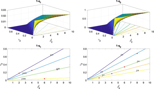
The probabilities $1-q_1$ and $1-q_2$ of a major epidemic when initiated by one individual from the low-susceptible or high-susceptible group, respectively, are graphed in Figure 8 as a function of transmission rate ${\beta }_2^S$ and recovery rate ${\gamma }_2$. Below these surfaces, are the contours for fixed probabilities. The surfaces and contours are computed from the BP approximation. To compare the values from the BP approximation to the CTMC models, a value is selected on each contour where ${\mathcal{R}}_0>1$. Ten thousand sample paths of the CTMC model are used to estimate the probability of a major epidemic. If the number of infected individuals $I_1+I_2$ reaches a total of 15 or greater, it is considered a major epidemic and if not it is considered a minor epidemic. The proportion (out of 10,000), where infected individuals reach 15 or greater is recorded as a dot on a contour and is listed in Table 8. The differences in the top two graphs in Figure 8 are only evident as a function of increasing recovery rate ${\gamma }_2$ (Theorem 4.2). The steep rise of $1-q_1$ or $1-q_2$ and sensitivity to the transmission rate ${\beta }_2^S$ can be clearly seen in these graphs. The transmission rate ${\beta }_2^S$ for group 2 increases the probability of a major epidemic when initiated with either an infected individual from a low-susceptible or a high-susceptible group (compare with the top left Figure 7.) We performed a sensitivity analysis of the basic reproduction number ${\mathcal{R}}_0$ (Equation (4(4) ${\mathcal{R}}_0=\frac{{\beta }_1^S}{{\gamma }_1}\frac{N_1}{N}+\frac{{\beta }_2^S}{{\gamma }_2}\frac{N_2}{N}.$(4) )) with respect to parameters ${\beta }_i^S$, i=1,2 (similar to the analysis in Table 6). The basic reproduction number ${\mathcal{R}}_0$ is much more sensitive to the parameters from group 2 (high-susceptible) than from group 1 (low-susceptible).

Figure 8. Probability of a major epidemic, $1-q_1$ and $1-q_2$, initiated by one low-susceptible individual or one high-susceptible individual, respectively, are graphed as a function of transmission rate (${\beta }_2^S$) and recovery rate (${\gamma }_2$) of the high-susceptible individuals. Other parameter values for measles are taken from Table 5. In addition, contours for each surface are graphed at the bottom of the figures, for several fixed probabilities.

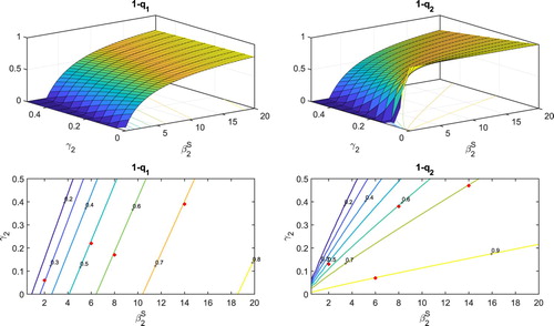
Table 8. The BP approximation of a major epidemic (either $1-q_1$ or $1-q_2$) is compared to the CTMC simulations based on 10,000 sample paths.

${\beta }_2^S$	${\gamma }_2$	$I_1\left(0\right)$	$I_2\left(0\right)$	BP	CTMC	${\mathcal{R}}_0$	${\mathcal{S}}_{{\beta }_1^S}^{{\mathcal{R}}_0}$	${\mathcal{S}}_{{\beta }_2^S}^{{\mathcal{R}}_0}$
2	0.06	1	0	0.300	0.288	3.693	1.330	12.31
6	0.22	1	0	0.500	0.499	3.087	1.111	8.420
8	0.17	1	0	0.600	0.606	5.066	1.824	23.84
14	0.39	1	0	0.700	0.696	3.950	1.422	14.18
2	0.13	0	1	0.500	0.525	1.899	0.683	2.921
6	0.07	0	1	0.900	0.904	3.937	3.215	76.55
8	0.38	0	1	0.600	0.595	2.465	0.888	5.190
14	0.47	0	1	0.700	0.699	3.339	1.202	9.945

Notes: The sensitivity indices ${\mathcal{S}}_p^{{\mathcal{R}}_0}$ for ${\mathcal{R}}_0$ are reported for parameters $p={\beta }_1^S$ and $p={\beta }_2^S$. Parameter values for measles are taken from Table 7.

The values of ${\mathcal{R}}_0$ in Table 8 are relatively small given the large values reported for measles in [17]. But the reproduction numbers for the high-susceptible group 2 are relatively large, i.e. ${\mathcal{R}}_{02}={\beta }_2^S/{\gamma }_2$ ranges from 15.4 to 85.7.

8. Discussion

Two CTMC SIR epidemic models with two groups are studied, where transmission depends either on the infectious individuals (Model 1) or susceptible individuals (Model 2). Model 1 is applicable to emerging diseases, new diseases which have not previously circulated in the population, such as SARS or MERS. It is assumed that all individuals are susceptible to infection. However, in Model 1, one group of individuals, known as superspreaders, transmit the disease to a large number of other individuals, whereas the remaining individuals have a much lower transmission rate and are referred to as non-superspreaders. Model 2 is applicable to re-emerging diseases, such as measles or pertussis. In Model 2, one group of individuals has immunity due to vaccination or to a prior infection of the disease and the second group has little or no immunity as individuals either have not been vaccinated or the vaccine has waned over time. The two groups are distinguished as either low- or high- susceptible groups, respectively.

A multitype BP approximation of the CTMC models is applied to the infected groups of individuals. It is shown analytically for Model 1, that the basic reproduction numbers within each group, ${\beta }_j^I/{\gamma }_j$, distinguish between the probability of a major or a minor epidemic for the two groups. If the outbreak is triggered by an infected superspreader, then there is a greater probability of a major epidemic than if initiated by a non-superspreader (Theorem 4.1). However, for Model 2, it is the recovery rates of the two susceptible groups that distinguishes which group has a greater probability of a major epidemic (Theorem 4.2). These analytical results are extended to an SEIR model with multiple latent stages and the results are confirmed in numerical simulations of the nonlinear CTMC models and exhibited in two applications, SARS (Model 1) and measles (Model 2), as illustrated in Figures 5–8. A major conclusion in this analysis is that ${\mathcal{R}}_0$ alone is insufficient to determine the probability of a major epidemic. Our analytical and numerical results demonstrate the importance of the heterogeneity in transmission and recovery rates in a large group of individuals and the transmission and recovery rates of the first individuals to become infected.

The two-group model can be extended to a multigroup model with $n\ge 2$ groups. For example, the extension of the basic reproduction number in (2(2) ${\mathcal{R}}_0=\sum _{i=1}^2\frac{{\beta }_i^m}{{\gamma }_i}\frac{N_i}{N}$(2) ) to a multigroup model is simply ${\mathcal{R}}_0=\sum _{i=1}^n\frac{{\beta }_i^m}{{\gamma }_i}\frac{N_i}{N}$ for m=I,S and Theorems 4.1 and 4.2 can be extended to n groups.

There are several limitations to the BP approximation of the CTMC epidemic models and to the model applications. To apply the BP approximation, the population size must be sufficiently large and second, the value of ${\mathcal{R}}_0$ must be greater than one and not too close to one. These restrictions ensure that it is possible to distinguish between a minor and major epidemic in the CTMC models. For many infectious diseases, transmission rates cannot be separated according to individual infectivity or susceptibility as in our two-group models. Populations are often highly heterogeneous and transmission rates may depend on both the infectiousness and the susceptibility of individuals within the population which in turn depend on behavioural, physiological, and environmental factors (e.g. [6,14,15,25,34]).

Acknowledgments

This research was partially supported by the National Science Foundation [grant number DMS-1517719]. We thank the reviewers and the editor for helpful suggestions on the original manuscript.

Disclosure statement

No potential conflict of interest was reported by the authors.

Additional information

Funding

National Science Foundation, 1517719.

Appendix 1. Probability generating functions for model 1

The pgf G for the branching process approximation is a function that defines the number of new infections given that the initial number infected is $I_1\left(0\right)=i_1$ and $I_2\left(0\right)=i_2$. The definition for G is $G_{(i_1,i_2)}(u_1,u_2,t)=\mathbb{E}\left(u_1^{I_1\left(t\right)}{u}_2^{I_2\left(t\right)}|I_1\left(0\right)=i_1,I_2\left(0\right)=i_2\right)=\sum _{(l,m)}{p}_{(i_1,i_2),(l,m)}\left(t\right)u_1^l{u}_2^m,$ where $\sum _{(l,m)}=\sum _{l=0}^{\mathrm{\infty }}\sum _{m=0}^{\mathrm{\infty }}$, $\mathbb{E}\left(X\right)$ denotes the expectation of X, and the transition probabilities $p_{(i_1,i_2),(l,m)}\left(t\right)=\mathbb{P}\left(I_1\right(t)=l,I_2(t)=m|I_1(0)=i_1,I_2(0)=i_2).$ The extinction probabilities are computed from G when $u_1=0=u_2$ with initial conditions $(i_1,i_2)=(1,0)$ and $p_{(1,0),(0,0)}\left(t\right)=G_{(1,0)}(0,0,t)$ or with $(i_1,i_2)=(0,1)$ and $p_{(0,1),(0,0)}\left(t\right)=G_{(0,1)}(0,0,t)$.

In the branching process approximation, it is assumed that the events are independent and thus, (A1) $G_{(i_1,i_2)}(u_1,u_2,t)={\left[G_{(1,0)}(u_1,u_2,t)\right]}^{i_1}\left[G_{(0,1)}\right(u_1,u_2,t){]}^{i_2}.$(A1) The preceding identity and the backward Kolmogorov differential equation are used to derive differential equations for the extinction probabilities.

Applying Table 3, the backward Kolmogorov differential equations for the transition probabilities of the branching process approximation for Model 1 have the following form (see, e.g. [3]): (A2) $\begin{array}{rl}\frac{\mathrm{d}{p}_{(i_1,i_2),(l,m)}\left(t\right)}{\mathrm{d}t}& =\left({\beta }_1^I{i}_1+{\beta }_2^I{i}_2\right)\frac{N_1}{N}{p}_{(i_1+1,i_2),(l,m)}\left(t\right)+\left({\beta }_1^I{i}_1+{\beta }_2^I{i}_2\right)\left(N_2/N\right)p_{(i_1,i_2+1),(l,m)}\left(t\right)\\ & +{\gamma }_1{i}_1{p}_{(i_1-1,i_2),(l,m)}\left(t\right)+{\gamma }_2{i}_2{p}_{(i_1,i_2-1),(l,m)}\left(t\right)\\ & -\left[\left({\beta }_1^I{i}_1+{\beta }_2^I{i}_2\right)\frac{N_1}{N}+\left({\beta }_1^I{i}_1+{\beta }_2^I{i}_2\right)\frac{N_2}{N}+{\gamma }_1{i}_1+{\gamma }_2{i}_2\right]p_{(i_1,i_2),(l,m)}\left(t\right).\end{array}$(A2) Differentiating Equation (A1(A1) $G_{(i_1,i_2)}(u_1,u_2,t)={\left[G_{(1,0)}(u_1,u_2,t)\right]}^{i_1}\left[G_{(0,1)}\right(u_1,u_2,t){]}^{i_2}.$(A1) ) with respect to t for $(i_1,i_2)=(1,0)$ and for $(i_1,i_2)=(0,1)$, and applying the definition and the identity (A1(A1) $G_{(i_1,i_2)}(u_1,u_2,t)={\left[G_{(1,0)}(u_1,u_2,t)\right]}^{i_1}\left[G_{(0,1)}\right(u_1,u_2,t){]}^{i_2}.$(A1) ) results in the following partial differential equations: (A3) $\frac{\mathrm{\partial }{G}_{(1,0)}}{\mathrm{\partial }t}=\frac{1}{i_1{G}_{(1,0)}^{i_1-1}}\frac{\mathrm{\partial }{G}_{(i_1,0)}}{\mathrm{\partial }t}=\frac{1}{i_1{G}_{(i_1-1,0)}}\sum _{(l,m)}\frac{\mathrm{d}{p}_{(i_1,0),(l,m)}}{\mathrm{d}t}{u}_1^l{u}_2^m$(A3) (A4) $\frac{\mathrm{\partial }{G}_{(0,1)}}{\mathrm{\partial }t}=\frac{1}{i_2{G}_{(0,1)}^{i_2-1}}\frac{\mathrm{\partial }{G}_{(0,i_2)}}{\mathrm{\partial }t}=\frac{1}{i_2{G}_{(0,i_2-1)}}\sum _{(l,m)}\frac{\mathrm{d}{p}_{(0,i_2),(l,m)}}{\mathrm{d}t}{u}_1^l{u}_2^m.$(A4) Substituting the backward Kolmogorov differential equations (A2(A2) $\begin{array}{rl}\frac{\mathrm{d}{p}_{(i_1,i_2),(l,m)}\left(t\right)}{\mathrm{d}t}& =\left({\beta }_1^I{i}_1+{\beta }_2^I{i}_2\right)\frac{N_1}{N}{p}_{(i_1+1,i_2),(l,m)}\left(t\right)+\left({\beta }_1^I{i}_1+{\beta }_2^I{i}_2\right)\left(N_2/N\right)p_{(i_1,i_2+1),(l,m)}\left(t\right)\\ & +{\gamma }_1{i}_1{p}_{(i_1-1,i_2),(l,m)}\left(t\right)+{\gamma }_2{i}_2{p}_{(i_1,i_2-1),(l,m)}\left(t\right)\\ & -\left[\left({\beta }_1^I{i}_1+{\beta }_2^I{i}_2\right)\frac{N_1}{N}+\left({\beta }_1^I{i}_1+{\beta }_2^I{i}_2\right)\frac{N_2}{N}+{\gamma }_1{i}_1+{\gamma }_2{i}_2\right]p_{(i_1,i_2),(l,m)}\left(t\right).\end{array}$(A2) ) into (A3(A3) $\frac{\mathrm{\partial }{G}_{(1,0)}}{\mathrm{\partial }t}=\frac{1}{i_1{G}_{(1,0)}^{i_1-1}}\frac{\mathrm{\partial }{G}_{(i_1,0)}}{\mathrm{\partial }t}=\frac{1}{i_1{G}_{(i_1-1,0)}}\sum _{(l,m)}\frac{\mathrm{d}{p}_{(i_1,0),(l,m)}}{\mathrm{d}t}{u}_1^l{u}_2^m$(A3) ) and applying the identity in (A1(A1) $G_{(i_1,i_2)}(u_1,u_2,t)={\left[G_{(1,0)}(u_1,u_2,t)\right]}^{i_1}\left[G_{(0,1)}\right(u_1,u_2,t){]}^{i_2}.$(A1) ) several times to simplify the expressions, we obtain the following differential equation for $G_{(1,0)}$: (A5) $\begin{array}{rl}\frac{\mathrm{\partial }{G}_{(1,0)}}{\mathrm{\partial }t}& =\frac{1}{G_{(i_1-1,0)}}\sum _{(l,m)}^{\mathrm{\infty }}\left[{\beta }_1^I\frac{N_1}{N}{p}_{(i_1+1,0),(l,m)}\left(t\right)+{\beta }_1^I\frac{N_2}{N}{p}_{(i_1,1),(l,m)}\left(t\right)+{\gamma }_1{p}_{(i_1-1,0),(l,m)}\left(t\right)\right.\\ & -\left.\left({\beta }_1^I\frac{N_1}{N}+{\beta }_1^I\frac{N_2}{N}+{\gamma }_1\right)p_{(i_1,0),(l,m)}\left(t\right)\right]u_1^l{u}_2^m\\ & =\frac{G_{(i_1+1,0)}}{G_{(i_1-1,0)}}{\beta }_1^I\frac{N_1}{N}+\frac{G_{(i_1,1)}}{G_{(i_1-1,0)}}{\beta }_1^I\frac{N_2}{N}+\frac{G_{(i_1-1,0)}}{G_{(i_1-1,0)}}{\gamma }_1\\ & -\frac{G_{(i_1,0)}}{G_{(i_1-1,0)}}\left[{\beta }_1^I\frac{N_1}{N}+{\beta }_1^I\frac{N_2}{N}+{\gamma }_1\right]\\ & =G_{(1,0)}^2{\beta }_1^I\frac{N_1}{N}+G_{(1,0)}{G}_{(0,1)}{\beta }_1^I\frac{N_2}{N}+{\gamma }_1-G_{(1,0)}({\beta }_1^I+{\gamma }_1)\\ & =({\beta }_1^I+{\gamma }_1)\left[f_1(G_{(1,0)},G_{(0,1)})-G_{(1,0)}\right],\end{array}$(A5) where $f_1$ is defined in (5(5) $f_1(u_1,u_2)=\frac{{\gamma }_1+{\beta }_1^I\frac{N_1}{N}{u}_1^2+{\beta }_1^I\frac{N_2}{N}{u}_1{u}_2}{{\gamma }_1+{\beta }_1^I},$(5) ). A similar derivation applies to the infected class $I_2$, after substituting (A2(A2) $\begin{array}{rl}\frac{\mathrm{d}{p}_{(i_1,i_2),(l,m)}\left(t\right)}{\mathrm{d}t}& =\left({\beta }_1^I{i}_1+{\beta }_2^I{i}_2\right)\frac{N_1}{N}{p}_{(i_1+1,i_2),(l,m)}\left(t\right)+\left({\beta }_1^I{i}_1+{\beta }_2^I{i}_2\right)\left(N_2/N\right)p_{(i_1,i_2+1),(l,m)}\left(t\right)\\ & +{\gamma }_1{i}_1{p}_{(i_1-1,i_2),(l,m)}\left(t\right)+{\gamma }_2{i}_2{p}_{(i_1,i_2-1),(l,m)}\left(t\right)\\ & -\left[\left({\beta }_1^I{i}_1+{\beta }_2^I{i}_2\right)\frac{N_1}{N}+\left({\beta }_1^I{i}_1+{\beta }_2^I{i}_2\right)\frac{N_2}{N}+{\gamma }_1{i}_1+{\gamma }_2{i}_2\right]p_{(i_1,i_2),(l,m)}\left(t\right).\end{array}$(A2) ) into (A4(A4) $\frac{\mathrm{\partial }{G}_{(0,1)}}{\mathrm{\partial }t}=\frac{1}{i_2{G}_{(0,1)}^{i_2-1}}\frac{\mathrm{\partial }{G}_{(0,i_2)}}{\mathrm{\partial }t}=\frac{1}{i_2{G}_{(0,i_2-1)}}\sum _{(l,m)}\frac{\mathrm{d}{p}_{(0,i_2),(l,m)}}{\mathrm{d}t}{u}_1^l{u}_2^m.$(A4) ): (A6) $\frac{\mathrm{\partial }{G}_{(0,1)}}{\mathrm{\partial }t}=({\beta }_2^I+{\gamma }_2)\left[f_2\right(G_{(1,0)},G_{(0,1)})-G_{(0,1)}],$(A6) where $f_2$ is defined in (6(6) $f_2(u_1,u_2)=\frac{{\gamma }_2+{\beta }_2^I\frac{N_2}{N}{u}_2^2+{\beta }_2^I\frac{N_1}{N}{u}_1{u}_2}{{\gamma }_2+{\beta }_2^I},$(6) ). The extinction probabilities $p_{(1,0),(0,0)}\left(t\right)$ and $p_{(0,1),(0,0)}\left(t\right)$ are the solutions of the differential equations in (A5(A5) $\begin{array}{rl}\frac{\mathrm{\partial }{G}_{(1,0)}}{\mathrm{\partial }t}& =\frac{1}{G_{(i_1-1,0)}}\sum _{(l,m)}^{\mathrm{\infty }}\left[{\beta }_1^I\frac{N_1}{N}{p}_{(i_1+1,0),(l,m)}\left(t\right)+{\beta }_1^I\frac{N_2}{N}{p}_{(i_1,1),(l,m)}\left(t\right)+{\gamma }_1{p}_{(i_1-1,0),(l,m)}\left(t\right)\right.\\ & -\left.\left({\beta }_1^I\frac{N_1}{N}+{\beta }_1^I\frac{N_2}{N}+{\gamma }_1\right)p_{(i_1,0),(l,m)}\left(t\right)\right]u_1^l{u}_2^m\\ & =\frac{G_{(i_1+1,0)}}{G_{(i_1-1,0)}}{\beta }_1^I\frac{N_1}{N}+\frac{G_{(i_1,1)}}{G_{(i_1-1,0)}}{\beta }_1^I\frac{N_2}{N}+\frac{G_{(i_1-1,0)}}{G_{(i_1-1,0)}}{\gamma }_1\\ & -\frac{G_{(i_1,0)}}{G_{(i_1-1,0)}}\left[{\beta }_1^I\frac{N_1}{N}+{\beta }_1^I\frac{N_2}{N}+{\gamma }_1\right]\\ & =G_{(1,0)}^2{\beta }_1^I\frac{N_1}{N}+G_{(1,0)}{G}_{(0,1)}{\beta }_1^I\frac{N_2}{N}+{\gamma }_1-G_{(1,0)}({\beta }_1^I+{\gamma }_1)\\ & =({\beta }_1^I+{\gamma }_1)\left[f_1(G_{(1,0)},G_{(0,1)})-G_{(1,0)}\right],\end{array}$(A5) ) and (A6(A6) $\frac{\mathrm{\partial }{G}_{(0,1)}}{\mathrm{\partial }t}=({\beta }_2^I+{\gamma }_2)\left[f_2\right(G_{(1,0)},G_{(0,1)})-G_{(0,1)}],$(A6) ) when $u_1=0=u_2$. Therefore, the probability of ultimate extinction, as $t\to \mathrm{\infty }$, given the initial data $\left(I_1\right(0),I_2(0\left)\right)=(1,0)$ or $\left(I_1\right(0),I_2(0\left)\right)=(0,1)$, is the steady-state solution of these equations, that is, the fixed points of the pgfs $f_1$ and $f_2$.

Appendix 2. Probability generating function for model 2

Applying Table 4, the backward Kolmogorov differential equations for the branching process approximation of Model 2 have the following form, e.g. [3]: (A7) $\begin{array}{rl}\frac{d{p}_{(i_1,i_2),(l,m)}\left(t\right)}{dt}& ={\beta }_1^S(i_1+i_2)\frac{N_1}{N}{p}_{(i_1+1,i_2),(l,m)}\left(t\right)+{\beta }_2^S(i_1+i_2)\frac{N_2}{N}{p}_{(i_1,i_2+1),(l,m)}\left(t\right)\\ & +{\gamma }_1{i}_1{p}_{(i_1-1,i_2),(l,m)}+{\gamma }_2{i}_2{p}_{(i_1,i_2-1),(l,m)}\left(t\right)\\ & -\left[{\beta }_1^S(i_1+i_2)\frac{N_1}{N}+{\beta }_2^S(i_1+i_2)\frac{N_2}{N}+{\gamma }_1{i}_1+{\gamma }_2{i}_2\right]p_{(i_1,i_2),(l,m)}\left(t\right).\end{array}$(A7) Applying the identities in (A3(A3) $\frac{\mathrm{\partial }{G}_{(1,0)}}{\mathrm{\partial }t}=\frac{1}{i_1{G}_{(1,0)}^{i_1-1}}\frac{\mathrm{\partial }{G}_{(i_1,0)}}{\mathrm{\partial }t}=\frac{1}{i_1{G}_{(i_1-1,0)}}\sum _{(l,m)}\frac{\mathrm{d}{p}_{(i_1,0),(l,m)}}{\mathrm{d}t}{u}_1^l{u}_2^m$(A3) ) and substituting the backward Kolmogorov differential equations (A7(A7) $\begin{array}{rl}\frac{d{p}_{(i_1,i_2),(l,m)}\left(t\right)}{dt}& ={\beta }_1^S(i_1+i_2)\frac{N_1}{N}{p}_{(i_1+1,i_2),(l,m)}\left(t\right)+{\beta }_2^S(i_1+i_2)\frac{N_2}{N}{p}_{(i_1,i_2+1),(l,m)}\left(t\right)\\ & +{\gamma }_1{i}_1{p}_{(i_1-1,i_2),(l,m)}+{\gamma }_2{i}_2{p}_{(i_1,i_2-1),(l,m)}\left(t\right)\\ & -\left[{\beta }_1^S(i_1+i_2)\frac{N_1}{N}+{\beta }_2^S(i_1+i_2)\frac{N_2}{N}+{\gamma }_1{i}_1+{\gamma }_2{i}_2\right]p_{(i_1,i_2),(l,m)}\left(t\right).\end{array}$(A7) ), yields the following differential equation for $G_{(1,0)}$: $\begin{array}{rl}\frac{\mathrm{\partial }{G}_{(1,0)}}{\mathrm{\partial }t}& =\frac{1}{G_{(i_1-1,0)}}\sum _{(l,m)}^{\mathrm{\infty }}\left[{\beta }_1^S\frac{N_1}{N}{p}_{(i_1+1,0),(l,m)}\left(t\right)+{\beta }_2^S\frac{N_2}{N}{p}_{(i_1,1),(l,m)}\left(t\right)+{\gamma }_1{p}_{(i_1-1,0),(l,m)}\left(t\right)\right.\\ & -\left.\left({\beta }_1^S\frac{N_1}{N}+{\beta }_1^S\frac{N_2}{N}+{\gamma }_1\right)p_{(i_1,0),(l,m)}\left(t\right)\right]u_1^l{u}_2^m\\ & =\frac{G_{(i_1+1,0)}}{G_{(i_1-1,0)}}{\beta }_1^S\frac{N_1}{N}+\frac{G_{(i_1,1)}}{G_{(i_1-1,0)}}{\beta }_1^S\frac{N_2}{N}+\frac{G_{(i_1-1,0)}}{G_{(i_1-1,0)}}{\gamma }_1\\ & -\frac{G_{(i_1,0)}}{G_{(i_1-1,0)}}({\beta }_1^S\frac{N_1}{N}+{\beta }_1^S\frac{N_2}{N}+{\gamma }_1)\\ & =\left({\beta }_1^S\frac{N_1}{N}+{\beta }_2^S\frac{N_2}{N}+{\gamma }_1\right)\left[f_1(G_{(1,0)},G_{(0,1)})-G_{(1,0)}\right].\end{array}$ Similarly using (A7(A7) $\begin{array}{rl}\frac{d{p}_{(i_1,i_2),(l,m)}\left(t\right)}{dt}& ={\beta }_1^S(i_1+i_2)\frac{N_1}{N}{p}_{(i_1+1,i_2),(l,m)}\left(t\right)+{\beta }_2^S(i_1+i_2)\frac{N_2}{N}{p}_{(i_1,i_2+1),(l,m)}\left(t\right)\\ & +{\gamma }_1{i}_1{p}_{(i_1-1,i_2),(l,m)}+{\gamma }_2{i}_2{p}_{(i_1,i_2-1),(l,m)}\left(t\right)\\ & -\left[{\beta }_1^S(i_1+i_2)\frac{N_1}{N}+{\beta }_2^S(i_1+i_2)\frac{N_2}{N}+{\gamma }_1{i}_1+{\gamma }_2{i}_2\right]p_{(i_1,i_2),(l,m)}\left(t\right).\end{array}$(A7) ) in (A4(A4) $\frac{\mathrm{\partial }{G}_{(0,1)}}{\mathrm{\partial }t}=\frac{1}{i_2{G}_{(0,1)}^{i_2-1}}\frac{\mathrm{\partial }{G}_{(0,i_2)}}{\mathrm{\partial }t}=\frac{1}{i_2{G}_{(0,i_2-1)}}\sum _{(l,m)}\frac{\mathrm{d}{p}_{(0,i_2),(l,m)}}{\mathrm{d}t}{u}_1^l{u}_2^m.$(A4) ) with $(i_1,i_2)=(0,1)$ yields $\frac{\mathrm{\partial }{G}_{(0,1)}}{\mathrm{\partial }t}=\left({\beta }_1^S\frac{N_1}{N}+{\beta }_2^S\frac{N_2}{N}+{\gamma }_2\right)\left[f_2(G_{(1,0)},G_{(0,1)})-G_{(0,1)}\right].$

Appendix 3. Probability generating functions for SEIR model

The pgfs for the general case of the SEIR model with m exposed stages and k groups is dependent on the variables $(u,v)=(u_{1,1},\dots ,u_{1,m},v_1,u_{2,1},\dots ,u_{2,m},v_k)$, where the u variables are for the exposed stages and the v variables are for the infected stages. In particular, the pgfs for each of the $E_{k,j}$ given $E_{k,j}\left(0\right)=1$ and the remaining exposed and infected states are initially zero are $\begin{array}{rl}{f}_{E_{k,j}}(u,v)& =\frac{{\alpha }_{k,j}{u}_{k,j+1}}{{\alpha }_{k,j}}=u_{k,j+1},j=1,2,\dots ,m-1\\ f_{E_{k,m}}(u,v)& =\frac{{\alpha }_{k,m}{v}_k}{{\alpha }_{k,m}}=v_k,j=m.\end{array}$ The pgf for $I_k$ when $I_k\left(0\right)=1$ and the remaining variables are initially zero in Model 1 is $f_{I_k}(u,v)=\frac{{\gamma }_k+{\beta }_k^I{v}_k\sum _{j=1}^2\frac{N_j}{N}{u}_{j,1}}{{\gamma }_k+{\beta }_k^I}.$ A similar expression applies to Model 2, $f_{I_k}(u,v)=\frac{{\gamma }_k+v_k\sum _{j=1}^2{\beta }_j^S\frac{N_j}{N}{u}_{j,1}}{{\gamma }_k+\sum _{j=1}^2{\beta }_j^S\frac{N_j}{N}}.$ As demonstrated in the previous two subsections, the backward Kolmogorov equations and assumptions regarding independence of the variables near the DFE leads to differential equations for the generating functions. For the special case of one exposed stage and two groups, let $E_{k,1}=E_k$, $e_{k,1}=e_k$ and ${\alpha }_{k,1}={\alpha }_k$. Then the generating function satisfies $G_{(e_1,i_1,e_2,i_2)}(u,v,t)=\left[G_{(1,0,0,0)}{]}^{e_1}\right[G_{(0,1,0,0)}{]}^{i_1}\left[G_{(0,0,1,0)}{]}^{e_2}\right[G_{(0,0,0,1)}{]}^{i_2}.$ In particular, (A8) $\begin{array}{rl}\frac{\mathrm{\partial }{G}_{(1,0,0,0)}}{\mathrm{\partial }t}& ={\alpha }_1\left[f_{E_1}\right(G_{(1,0,0,0)},\dots ,G_{(0,0,0,1)})-G_{(1,0,0,0)}]={\alpha }_1[G_{(0,1,0,0)}-G_{(1,0,0,0)}],\\ \frac{\mathrm{\partial }{G}_{(0,0,1,0)}}{\mathrm{\partial }t}& ={\alpha }_2\left[f_{E_2}\right(G_{(1,0,0,0)},\dots ,G_{(0,0,0,1)})-G_{(0,0,1,0)}]={\alpha }_2[G_{(0,0,0,1)}-G_{(0,0,1,0)}].\end{array}$(A8) Evaluating the generating function G when the u and v variables are zero gives the probability of extinction starting from either $E_1\left(0\right)=1$ ($p_{(1,0,0,0),(0,0,0,0)}\left(t\right)$) or $E_2\left(0\right)=1$ ($p_{(0,0,1,0),(0,0,0,0)}\left(t\right)$). The probability of ultimate extinction is the fixed point of these pgfs. Therefore, it follows from the expressions in (A8(A8) $\begin{array}{rl}\frac{\mathrm{\partial }{G}_{(1,0,0,0)}}{\mathrm{\partial }t}& ={\alpha }_1\left[f_{E_1}\right(G_{(1,0,0,0)},\dots ,G_{(0,0,0,1)})-G_{(1,0,0,0)}]={\alpha }_1[G_{(0,1,0,0)}-G_{(1,0,0,0)}],\\ \frac{\mathrm{\partial }{G}_{(0,0,1,0)}}{\mathrm{\partial }t}& ={\alpha }_2\left[f_{E_2}\right(G_{(1,0,0,0)},\dots ,G_{(0,0,0,1)})-G_{(0,0,1,0)}]={\alpha }_2[G_{(0,0,0,1)}-G_{(0,0,1,0)}].\end{array}$(A8) ) that the probability of ultimate extinction beginning from $E_k\left(0\right)=1$ is the same as for $I_k\left(0\right)=1$ for k=1, 2.

Appendix 4. Proof of Theorem 4.1

In multitype continuous-time branching processes, the probability of ultimate extinction is the minimal fixed point of the system of pgfs in the unit square, $[0,1]\times [0,1]$ (e.g. [2,4,5,18]). Suppose the fixed points of the pgfs for the BP approximation in (5(5) $f_1(u_1,u_2)=\frac{{\gamma }_1+{\beta }_1^I\frac{N_1}{N}{u}_1^2+{\beta }_1^I\frac{N_2}{N}{u}_1{u}_2}{{\gamma }_1+{\beta }_1^I},$(5) ) and (6(6) $f_2(u_1,u_2)=\frac{{\gamma }_2+{\beta }_2^I\frac{N_2}{N}{u}_2^2+{\beta }_2^I\frac{N_1}{N}{u}_1{u}_2}{{\gamma }_2+{\beta }_2^I},$(6) ) are $(q_1,q_2)$ which are the solutions of the equations $f_1(u_1,u_2)=u_1$ and $f_2(u_1,u_2)=u_2$: (A9) $\frac{{\gamma }_1+{\beta }_1^I\frac{N_1}{N}{u}_1^2+{\beta }_1^I\frac{N_2}{N}{u}_1{u}_2}{{\gamma }_1+{\beta }_1^I}=u_1,$(A9) (A10) $\frac{{\gamma }_2+{\beta }_2^I\frac{N_2}{N}{u}_2^2+{\beta }_2^I\frac{N_1}{N}{u}_1{u}_2}{{\gamma }_2+{\beta }_2^I}=u_2.$(A10) Rearranging the preceding equations gives two curves: (A11) $u_2=\frac{{\gamma }_1+{\beta }_1^I}{{\beta }_1^I}\frac{N}{N_2}-\frac{{\gamma }_1}{{\beta }_1^I}\frac{N}{N_2}\frac{1}{u_1}-\frac{N_1}{N_2}{u}_1=g_1\left(u_1\right),$(A11) (A12) $u_1=\frac{{\gamma }_2+{\beta }_2^I}{{\beta }_2^I}\frac{N}{N_1}-\frac{{\gamma }_2}{{\beta }_2^I}\frac{N}{N_1}\frac{1}{u_2}-\frac{N_2}{N_1}{u}_2=g_2\left(u_2\right).$(A12) The curve $g_1$ intersects the line $u_2=u_1$ at two points: $(1,1)$ and $({\gamma }_1/{\beta }_1^I,{\gamma }_1/{\beta }_1^I)$ and the curve $g_2$ intersects the line $u_2=u_1$ at $(1,1)$ and $({\gamma }_2/{\beta }_2^I,{\gamma }_2/{\beta }_2^I)$, where both points may or may not lie in the set $[0,1]\times [0,1]$. In addition, function $g_1$ in (A11(A11) $u_2=\frac{{\gamma }_1+{\beta }_1^I}{{\beta }_1^I}\frac{N}{N_2}-\frac{{\gamma }_1}{{\beta }_1^I}\frac{N}{N_2}\frac{1}{u_1}-\frac{N_1}{N_2}{u}_1=g_1\left(u_1\right),$(A11) ) is concave down with respect to $u_1\in [0,1]$ and function $g_2$ in (A12(A12) $u_1=\frac{{\gamma }_2+{\beta }_2^I}{{\beta }_2^I}\frac{N}{N_1}-\frac{{\gamma }_2}{{\beta }_2^I}\frac{N}{N_1}\frac{1}{u_2}-\frac{N_2}{N_1}{u}_2=g_2\left(u_2\right).$(A12) ) is concave down with respect to $u_2\in [0,1]$.

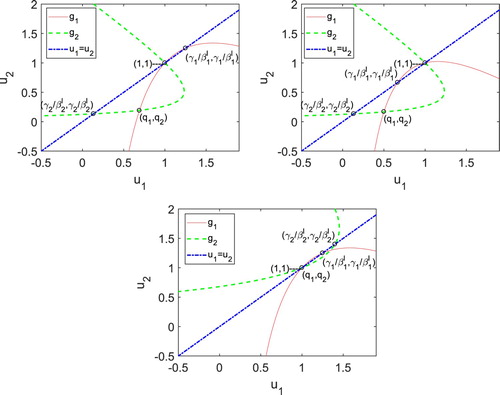
To verify Theorem 4.1, three cases are considered (i) ${\mathcal{R}}_0>$ 1 with ${\beta }_1^I/{\gamma }_1<1$ and ${\beta }_2^I/{\gamma }_2>1$; (ii) ${\mathcal{R}}_0>1$ with ${\beta }_1^I/{\gamma }_1>1$ and ${\beta }_2^I/{\gamma }_2>1$; (iii) ${\mathcal{R}}_0\le$ 1 with ${\beta }_1^I/{\gamma }_1\le$ 1 and ${\beta }_2^I/{\gamma }_2\le 1$. See Figure A1 for the three cases.

1. Assume ${\mathcal{R}}_0>1$ with ${\beta }_1^I/{\gamma }_1<1$ and ${\beta }_2^I/{\gamma }_2>1$. Curve $g_1$ in (A11(A11) $u_2=\frac{{\gamma }_1+{\beta }_1^I}{{\beta }_1^I}\frac{N}{N_2}-\frac{{\gamma }_1}{{\beta }_1^I}\frac{N}{N_2}\frac{1}{u_1}-\frac{N_1}{N_2}{u}_1=g_1\left(u_1\right),$(A11) ) intersects the line $u_2=u_1$ only at (1,1) in the unit square, $({\gamma }_1/{\beta }_1^I,{\gamma }_1/{\beta }_1^I)\notin [0,1]\times [0,1]$. Curve $g_2$ in equation (A12(A12) $u_1=\frac{{\gamma }_2+{\beta }_2^I}{{\beta }_2^I}\frac{N}{N_1}-\frac{{\gamma }_2}{{\beta }_2^I}\frac{N}{N_1}\frac{1}{u_2}-\frac{N_2}{N_1}{u}_2=g_2\left(u_2\right).$(A12) ) intersects the line at $(1,1)$ and $({\gamma }_2/{\beta }_2^I,{\gamma }_2/{\beta }_2^I)$ inside the unit square. The two curves $g_1$ and $g_2$ intersect inside the unit square (minimal fixed point) iff $\left(d{g}_1/d{u}_1\right){|}_{u_1=1}>1>\left(d{g}_2/d{u}_2\right){|}_{u_2=1}$ iff ${\mathcal{R}}_0>1$. Therefore, from the order of the intersections of the curves with the line ${\gamma }_2/{\beta }_2^I<1<{\gamma }_1/{\beta }_1^I$ and the properties of $g_1$ and $g_2$, the fixed point must lie below the line ( Figure A1(i)). Hence, the minimal fixed point satisfies $q_1>q_2$.

2. Assume ${\mathcal{R}}_0>1$ with ${\beta }_1^I/{\gamma }_1>1$ and ${\beta }_2^I/{\gamma }_2>1$. Curve $g_1$ in Equation (A11(A11) $u_2=\frac{{\gamma }_1+{\beta }_1^I}{{\beta }_1^I}\frac{N}{N_2}-\frac{{\gamma }_1}{{\beta }_1^I}\frac{N}{N_2}\frac{1}{u_1}-\frac{N_1}{N_2}{u}_1=g_1\left(u_1\right),$(A11) ) intersects the line $u_2=u_1$ at $(1,1)$ and (${\gamma }_1/{\beta }_1^I,{\gamma }_1/{\beta }_1^I$). Both points lie in the unit square. Similarly, curve $g_2$ in Equation (A12(A12) $u_1=\frac{{\gamma }_2+{\beta }_2^I}{{\beta }_2^I}\frac{N}{N_1}-\frac{{\gamma }_2}{{\beta }_2^I}\frac{N}{N_1}\frac{1}{u_2}-\frac{N_2}{N_1}{u}_2=g_2\left(u_2\right).$(A12) ) intersects the line at (1,1) and $({\gamma }_2/{\beta }_2^I,{\gamma }_2/{\beta }_2^I)$. Since ${\gamma }_2/{\beta }_2^I<{\gamma }_1/{\beta }_1^I<1$, the shape of the curves on the unit square imply the minimal fixed point must lie below the line $u_2=u_1$. Hence, $q_1>q_2$.

3. Assume ${\mathcal{R}}_0\le$ 1 with ${\beta }_1^I/{\gamma }_1\le$ 1 and ${\beta }_2^I/{\gamma }_2\le 1$. In $[0,1]\times [0,1]$, the curves $g_1$ and $g_2$ intersect $u_2=u_1$ only at the point $(1,1)$. Thus, $q_2=q_1=1$. See Figure A1(iii).

In the special case, ${\beta }_1^I/{\gamma }_1={\beta }_2^I/{\gamma }_2=\beta /\gamma$, then ${\mathcal{R}}_0=\beta /\gamma$. The curve $g_1\left(u_1\right)$ $(=g_2(u_2\left)\right)$ intersects $u_2=u_1$ at (1,1) and ($\beta /\gamma ,\beta /\gamma$). Therefore, $q_1=1/{\mathcal{R}}_0=q_2$.

Appendix 5. Proof of Theorem 4.2

Suppose the fixed points of the pgfs are $(q_1,q_2)$. Consider the functions $f_1(u_1,u_2)=u_1$ and $f_2(u_1,u_2)=u_2$ given in Equations (7(7) $f_1(u_1,u_2)=\frac{{\gamma }_1+{\beta }_1^S\frac{N_1}{N}{u}_1^2+{\beta }_2^S\frac{N_2}{N}{u}_1{u}_2}{{\gamma }_1+{\beta }_1^S\frac{N_1}{N}+{\beta }_2^S\frac{N_2}{N}},$(7) ) and (8(8) $f_2(u_1,u_2)=\frac{{\gamma }_2+{\beta }_2^S\frac{N_2}{N}{u}_2^2+{\beta }_1^S\frac{N_1}{N}{u}_1{u}_2}{{\gamma }_2+{\beta }_2^S\frac{N_2}{N}+{\beta }_1^S\frac{N_1}{N}},$(8) ), respectively, (A13) $\frac{{\gamma }_1+{\beta }_1^S\frac{N_1}{N}{u}_1^2+{\beta }_2^S\frac{N_2}{N}{u}_1{u}_2}{{\gamma }_1+{\beta }_1^S\frac{N_1}{N}+{\beta }_2^S\frac{N_2}{N}}=u_1,$(A13) (A14) $\frac{{\gamma }_2+{\beta }_2^S\frac{N_2}{N}{u}_2^2+{\beta }_1^S\frac{N_1}{N}{u}_1{u}_2}{{\gamma }_2+{\beta }_1^S\frac{N_1}{N}+{\beta }_2^S\frac{N_2}{N}}=u_2.$(A14) Rewriting Equation (A13(A14) $\frac{{\gamma }_2+{\beta }_2^S\frac{N_2}{N}{u}_2^2+{\beta }_1^S\frac{N_1}{N}{u}_1{u}_2}{{\gamma }_2+{\beta }_1^S\frac{N_1}{N}+{\beta }_2^S\frac{N_2}{N}}=u_2.$(A14) ) and (A14(A13) $\frac{{\gamma }_1+{\beta }_1^S\frac{N_1}{N}{u}_1^2+{\beta }_2^S\frac{N_2}{N}{u}_1{u}_2}{{\gamma }_1+{\beta }_1^S\frac{N_1}{N}+{\beta }_2^S\frac{N_2}{N}}=u_1,$(A13) ): (A15) $u_2=\frac{{\gamma }_1}{{\beta }_2^S}\frac{N}{N_2}+\frac{{\beta }_1^S}{{\beta }_2^S}\frac{N_1}{N_2}+1-\frac{{\gamma }_1}{{\beta }_2^S}\frac{N}{N_2}\frac{1}{u_1}-\frac{{\beta }_1^S}{{\beta }_2^S}\frac{N_1}{N_2}{u}_1=h_1\left(u_1\right),$(A15) (A16) $u_1=\frac{{\gamma }_2}{{\beta }_1^S}\frac{N}{N_1}+\frac{{\beta }_2^S}{{\beta }_1^S}\frac{N_2}{N_1}+1-\frac{{\gamma }_2}{{\beta }_1^S}\frac{N}{N_1}\frac{1}{u_2}-\frac{{\beta }_2^S}{{\beta }_1^S}\frac{N_2}{N_1}{u}_2=h_2\left(u_2\right).$(A16) The functions $h_1$ and $h_2$ have the same properties as the functions $g_1$ and $g_2$, similar to the proof of Theorem 4.1 in Appendix 4. Functions $h_1$ and $h_2$ are both concave down with respect to the axes $u_1$ and $u_2$, respectively, the curve $h_1$ intersects the line $u_2=u_1$ at $(1,1)$, and (A17) $\left(\frac{{\gamma }_{1}N}{N_1{\beta }_1^S+N_2{\beta }_2^S},\frac{{\gamma }_{1}N}{N_1{\beta }_1^S+N_2{\beta }_2^S}\right).$(A17) The curve $h_2$ intersects the line $u_2=u_1$ at $(1,1)$ and (A18) $\left(\frac{{\gamma }_{2}N}{N_1{\beta }_1^S+N_2{\beta }_2^S},\frac{{\gamma }_{2}N}{N_1{\beta }_1^S+N_2{\beta }_2^S}\right).$(A18) Notice that the difference between the two points in (A17(A17) $\left(\frac{{\gamma }_{1}N}{N_1{\beta }_1^S+N_2{\beta }_2^S},\frac{{\gamma }_{1}N}{N_1{\beta }_1^S+N_2{\beta }_2^S}\right).$(A17) ) and (A18(A18) $\left(\frac{{\gamma }_{2}N}{N_1{\beta }_1^S+N_2{\beta }_2^S},\frac{{\gamma }_{2}N}{N_1{\beta }_1^S+N_2{\beta }_2^S}\right).$(A18) ) is the recovery rates, ${\gamma }_1$ and ${\gamma }_2$. We assume ${\gamma }_1>{\gamma }_2$. The proof follows in a manner similar to Theorem 4.1 by noting the order of the points of intersections of the curves $h_1$ and $h_2$ with the line $u_2=u_1.$ Similar to Theorem 4.1 in Appendix 4, when ${\gamma }_1>{\gamma }_2$ we consider two different cases: (i) ${\mathcal{R}}_0>1$ and (ii) ${\mathcal{R}}_0\le 1$.

Since ${\gamma }_1>{\gamma }_2$, $\left({\gamma }_{1}N/(N_1{\beta }_1^S+N_2{\beta }_2^S)\right)>\left(1/{\mathcal{R}}_0\right)>\left({\gamma }_{2}N/(N_1{\beta }_1^S+N_2{\beta }_2^S)\right)$. In the first case (i) when ${\mathcal{R}}_0>1$, $q_1=min\{1,({\gamma }_{1}N/\left(N_1{\beta }_1^S+N_2{\beta }_2^S\right)\left)\right\}$ and $q_2=\left({\gamma }_{2}N/(N_1{\beta }_1^S+N_2{\beta }_2^S)\right)$ is less than one. So $q_1>q_2$. In the second case (ii) when ${\mathcal{R}}_0\le 1$, ${\beta }_1^S/{\gamma }_1^S\le 1$ and ${\beta }_2^S/{\gamma }_2^S\le 1$. So $\left({\gamma }_{1}N/(N_1{\beta }_1^S+N_2{\beta }_2^S)\right)>\left({\gamma }_{2}N/(N_1{\beta }_1^S+N_2{\beta }_2^S)\right)>1$. Hence, $h_1$ and $h_2$ intersect $u_2=u_1$ only at (1, 1), so $q_1=1=q_2$.

In the special case that ${\gamma }_1={\gamma }_2$, the two curves, $h_1$ and $h_2$, have two points of intersection, namely $(1,1)$ and $(1/{\mathcal{R}}_0,1/{\mathcal{R}}_0)$ where this latter fixed point is the expression given in (A17(A17) $\left(\frac{{\gamma }_{1}N}{N_1{\beta }_1^S+N_2{\beta }_2^S},\frac{{\gamma }_{1}N}{N_1{\beta }_1^S+N_2{\beta }_2^S}\right).$(A17) ) or in (A18(A18) $\left(\frac{{\gamma }_{2}N}{N_1{\beta }_1^S+N_2{\beta }_2^S},\frac{{\gamma }_{2}N}{N_1{\beta }_1^S+N_2{\beta }_2^S}\right).$(A18) ). If ${\mathcal{R}}_0>1$, then $q_1=1/{\mathcal{R}}_0=q_2$ and if ${\mathcal{R}}_0\le 1$, then $q_1=q_2=1.$

Figure A1. Curves $g_1$, $g_2$ and the line $u_2=u_1$ in cases (i), (ii) and (iii). (a) Case (i). (b) Case (ii). (c) Case (iii).

References

- L.J.S. Allen, An Introduction to Stochastic Processes with Applications to Biology, 2nd ed., CRC Press, Boca Raton, Fl., 2010.
- L.J.S. Allen, Stochastic Population and Epidemic Models Persistence and Extinction, Springer International Publishing, Switzerland, 2015.
- L.J.S. Allen, A primer on stochastic epidemic models: Formulation, numerical simulation, and analysis, Infect. Dis. Model. 2 (2017), pp. 128–142.
- L.J.S. Allen and P. van den Driessche, Relations between deterministic and stochastic thresholds for disease extinction in continuous- and discrete-time infectious disease models, Math. Biosci. 243 (2013), pp. 99–108. doi: 10.1016/j.mbs.2013.02.006
- K.B. Athreya and A.P. Ney, Branching Processes, Springer-Verlag, New York, 1972.
- L. Bolzoni, L. Real, and G. De Leo, Transmission heterogeneity and control strategies for infectious disease emergence, PLoS. One 2 (2007), pp. 747. Available at https://doi.org/10.1371/journal.pone.0000747.
- N. Chitnis, J.M. Hyman, and J.M. Cushing, Determining important parameters in the spread of malaria through the sensitivity analysis of a mathematical model, Bull. Math. Biol. 70 (2008), pp. 1272–1296. doi: 10.1007/s11538-008-9299-0
- S.Y. Cho, J. Kang, Y.E. Ha, G.E. Park, J.Y. Lee, J.H. Ko, J.Y. Lee, J.M. Kim, C. Kang, I.J. Jo, J.G. Ryu, J.R. Choi, S. Kim, H.J. Huh, C.S. Ki, E.S. Kang, K.R. Peck, H.J. Dhong, J.H. Song, D.R.Chung, and Y.J. Kim, MERS-CoV outbreak following a single patient exposure in an emergency room in South Korea: An epidemiological outbreak study, Lancet 388 (2016), pp. 994–1001. doi: 10.1016/S0140-6736(16)30623-7
- G. Chowell, S. Blumberg, L. Simonsen, M. Miller, and C. Viboud, Synthesizing data and models for the spread of MERS-CoV, 2013: Key role of index cases and hospital transmission, Epidemics 9 (2014), pp. 40–51. doi: 10.1016/j.epidem.2014.09.011
- G. Chowell, C. Castillo-Chavez, P.W. Fenimore, C.M. Kribs-Zaleta, L. Arriola, and J.M. Hyman, Model parameters and outbreak control for SARS, Emerg. Infect. Dis. 10 (2004), pp. 1258–1263. doi: 10.3201/eid1007.030647
- G. De Serres, N. Boulianne, N. Brousseau, M. Benoit, S. Lacoursiere, F. Guillemette, J. Soto, M.Ouakki, B. Ward, and D. Skowronski, Higher risk of measles when the first dose of a 2-dose schedule of measles vaccine is given at 12–14 months versus 15 months of age, Clin. Infect. Dis. 55 (2012), pp. 394–402. doi: 10.1093/cid/cis439
- O. Diekmann, J. Heesterbeek, and J. Metz, On the definition and the computation of the basic reproduction ratio R0 in models for infectious diseases in heterogeneous populations, J. Math. Biol. 28 (1990), pp. 365–382. doi: 10.1007/BF00178324
- C.J. Edholm, B.O. Emerenini, A.L. Murillo2018 Searching for superspreaders: Identifying epidemic patterns associated with superspreading events in stochastic models, in Understanding Complex Biological Systems with Mathematics, Chapter 1, pp. 1–29, Springer Nature, Switzerland
- Z. Feng, A.N. Hill, A.T. Curns, and J.W. Glasser, Evaluating targeted interventions via meta-population models with multi-level mixing, Math. Biosci. 287 (2017), pp. 93–104. doi: 10.1016/j.mbs.2016.09.013
- A.P. Galvani and R.M. May, Dimensions of superspreading, Nature 438 (2005), pp. 293–295. doi: 10.1038/438293a
- G. Gopalakrishna, P. Choo, Y. Leo, B.K. Tay, Y.T. Lim, A.S. Khan, and C.C. Tan, SARS transmission and hospital containment, Emerg. Infect. Dis. 10 (2004), pp. 395–400. doi: 10.3201/eid1003.030650
- F.M. Guerra, S. Bolotin, G. Lim, J. Heffernan, S.L. Deeks, Y. Li, and N.S. Crowcroft, The basic reproduction number (R0) of measles: A systematic review, Lancet Infect. Dis. 17 (2017), pp. e420–e428. doi: 10.1016/S1473-3099(17)30307-9
- T.E. Harris, The Theory of Branching Processes, Springer-Verlag, Berlin, Heidelberg, 1963.
- H. Hethcote, The mathematics of infectious disease, SIAM Rev. 42 (2000), pp. 599–653. doi: 10.1137/S0036144500371907
- A. James, J.W. Pitchford, and M.J. Plank, An event-based model of superspreading in epidemics, Proc. R. Soc. Lond. [Biol] 274 (2007), pp. 741–747. doi: 10.1098/rspb.2006.0219
- S. Karlin and H. Taylor, A Second Course in Stochastic Processes, Academic Press, New York, 1981.
- M. Kontio, S. Jokinen, M. Paunio, H. Peltola, and I. Davidkin, Waning antibody levels and avidity: Implications for MMR vaccine-induced protection, J. Infect. Dis. 206 (2012), pp. 1542–1548. doi: 10.1093/infdis/jis568
- J.W. Leavitt, Typhoid Mary: Captive to the Public's Health, Beacon Press, Boston, 1996.
- J. Lee, G. Chowell, and E. Jung, A dynamic compartmental model for the Middle East respiratory syndrome outbreak in the Republic of Korea: A retrospective analysis on control interventions and superspreading events., J. Theoret. Biol. 408 (2016), pp. 118–126. doi: 10.1016/j.jtbi.2016.08.009
- J.O. Lloyd-Smith, S.J. Schreiber, P.E. Kopp, and W.M. Getz, Superspreading and the effect of individual variation on disease emergence, Nature 438 (2005), pp. 355–359. doi: 10.1038/nature04153
- P. Magal, O. Seydi, and G. Webb, Final size of an epidemic for a two group SIR model, SIAM J. Appl. Math. 76 (2016), pp. 2042–2059. doi: 10.1137/16M1065392
- T. Mkhatshwa and A. Mummert, Modeling super-spreading events for infectious disease: Case study SARS, Int. J. Acad. Med. 41 (2011), pp. 82–88. doi: 10.1111/j.1445-5994.2010.02339.x
- National Center for Immunization and Respiratory Diseases, Epidemiology and prevention of vaccine-preventable diseases. Available at https://www.cdc.gov/vaccines/pubs/pinkbook/meas.html (last access date 2/1/2018).
- National Center for Immunization and Respiratory Diseases, Division of Viral Diseases, Severe Acute Respiratory Syndrome (SARS). Available at https://www.cdc.gov/sars/about/faq.html (last access date 2/1/2018).
- National Institutes of Health (US), Biological Sciences Curriculum Study, Bethesda (MD). Available at https://www.ncbi.nlm.nih.gov/books/nbk20370/ (last access date 2/1/2018).
- N.I. Nii-Trebi, Emerging and neglected infectious diseases: Insights, advances, and challenges, Biomed. Res. Int. 2017 (2017), pp. ID 5245021, 15 pages. doi: 10.1155/2017/5245021
- E. Rothstein and K. Edwards, Health burden of pertussis in adolescents and adults, Pediatr. Infect. Dis. J. 24 (2005), pp. S44–S47. doi: 10.1097/01.inf.0000160912.58660.87
- Z. Shen, F. Ning, W. Zhou, X. He, C. Lin, D.P. Chin, Z. Zhu, and A. Schuchat, Superspreading SARS events, Beijing 2003, Emerg. Infect. Dis. 10 (2004), pp. 256–260. doi: 10.3201/eid1002.030732
- R.A. Stein, Super-spreaders in infectious diseases, Int. J. Infect. Dis. 15 (2011), pp. e510–e513. Available at https://www.ncbi.nlm.nih.gov/pubmed/21737332. doi: 10.1016/j.ijid.2010.06.020
- A.J. Tatem, D.J. Rodgers, and S.I. Hay, Global transport networks and infectious disease spread, Adv. Parasit. 62 (2006), pp. 293–343. doi: 10.1016/S0065-308X(05)62009-X
- P. van den Driessche and J. Watmough, Reproduction numbers and sub-threshold endemic equilibria for compartmental models of disease transmission, Math. Biosci. 180 (2002), pp. 29–48. doi: 10.1016/S0025-5564(02)00108-6
- J. Wallinga and P. Teunis, Different epidemic curves for severe acute respiratory syndrome reveal similar impacts of control measures, Amer. J. Epidemiol. 160 (2004), pp. 509–516. doi: 10.1093/aje/kwh255
- A.M. Wendelboe, A. van Rie, S. Salmaso, and J.A. Englund, Duration of immunity against pertussis after natural infection or vaccination, Pediatr. Infect. Dis. J. 24 (2005), pp. S58–S61. doi: 10.1097/01.inf.0000160914.59160.41
- P. Whittle, The outcome of a stochastic epidemic: A note on Bailey's paper, Biometrika 42 (1955), pp. 116–122.
- G. Wong, W. Liu, Y. Liu, B. Zhou, Y. Bi, and G.F. Gao, MERS, SARS, and Ebola: The role of super-spreaders in infectious disease, Cell Host Microbe 18 (2015), pp. 398–401. doi: 10.1016/j.chom.2015.09.013