Combination of singularly perturbed vector field method and method of directly defining the inverse mapping applied to complex ODE system prostate cancer model

ABSTRACT

We propose a new method to solve a system of complex ordinary differential equations (ODEs) with hidden hierarchy. Given a complex system of the ODE, the hierarchy of the system is generally hidden. Once we reveal the hierarchy of the system, the system can be reduced into subsystems called slow and fast subsystems. This division of slow and fast subsystems reduces the analysis and hence reduces the computation time, which can be expensive. In our new method, we first apply the singularly perturbed vector field method that is the global quasi-linearization method. This method exposes the hierarchy of a given complex system. Subsequently, we apply a version of the homotopy analysis method called the method of directly defining the inverse mapping. We applied our new method to the immunotherapy of advanced prostate cancer.

KEYWORDS:

• Semi-analytical method
• prostate cancer
• PSA
• immunotherapy
• tumour
• ordinary differential equations

2010 MATHEMATICS SUBJECT CLASSIFICATIONS:

• Mathematical Biology Model
• Asymptotic Analysis
• Qualitative theory

1. Introduction

Prostate cancer is typical among men over 50, and diagnosis among young people is rare. Unlike other cancers, prostate cancer cells are common. Prostate cancer can remain unchanged for a long time. Thus approximately one-third of men over the age of 50, and the vast majority of men over the age of 80, have cancer cells in the prostate. Prostate cancer grows extremely slowly; among the elderly especially, it often does not cause any symptoms. However, prostate cancer can grow rapidly and even spread to other organs in the body, especially to the bones [2]. In the early stages, prostate cancer does not cause symptoms and does not exhibit any external signs. Symptoms appear when the tumour grows and places pressure on the urethral tube. Since prostate cancer grows slowly, the onset of symptoms can occur years after the tumour has appeared. Typical symptoms are difficulty in urinating, increased urinary frequency, especially at night, pain during urination, blood in urine or sexual contact (rare). If cancer has metastasized to the bones, bone pain is experienced. Sometimes, the first symptoms felt are muscle pain in the back, hips or pelvis. The initial diagnosis is a visit to a family doctor who performs a rectal finger test, PSA test, trans-rectal ultrasound and biopsy.

When the prostate cancer is at the advanced stage, it is more aggressive and spreads further throughout the body. In this case, the treatment required is chemotherapy, androgen deprivation therapy (ADT) or androgen suppression therapy, which is a hormonal treatment that reduces the effect of androgen. Androgens are male hormones that can stimulate cancer growth. ADT can decelerate and even stop cancer growth by decreasing androgen levels. ADT therapy reduces androgen-dependent (AD) cancer cells by preventing growth and inducing apoptosis [18]. At this hormone refractory stage, the AD cells are replaced by androgen-independent (AI) cells. These cells do not require the normal levels of androgen to sustain growth and are also resistant to the apoptotic effect of a low-androgen environment. In some cases, an alternative therapy treatment called intermittent androgen deprivation (IAD) is used [1]. The advantage of this treatment is the availability of an off-treatment period to the patients that provides some relief from treatment-related side effects and reduces treatment costs. In addition, IAD may also delay the progression to castration-resistant prostate cancer. Immunotherapy dendritic vaccines (dendritic cell (DC) vaccines)-based vaccination is a treatment for harnessing the potential of a patients own immune system to eliminate tumour cells in metastatic hormone-refractory cancer. Patients that are treated by immunotherapy dendritic vaccines develop an immune response following vaccination. Some patients experience a significant decline in their PSA level, and others experience stabilization of their previous progressing disease [19, 21, 22].

A mathematical model of prostate cancer during androgen suppression was first proposed by [9, 10]. Later, the first mathematical model of prostate cancer under IAS was proposed by [8]. Their model was extended to a model with partial differential equations [7, 24, 25], and a model with competition between different classes of prostate tumour cells [23]. However, these models share a typical drawback: they cannot describe the biphasic decline in PSA during the on-treatment periods. The authors of the paper [5] evaluated the probability of death by prostate cancer under various treatment options using a cell kinetic model. In the paper [13], the authors proposed a mathematical model for the immunotherapy of prostate cancer.

The model in the paper [8] has been further extended to allow many key parameters to be functions of the cell androgen content [20]. Other groups of researchers have considered more detailed biochemical dynamics of androgen and androgen receptors, and the related effects [6, 11].

All these mathematical models are described by a system of linear or nonlinear ordinary differential equations (ODEs) or partial differential equations (PDE). In general, a set of differential equations describing a complex realistic phenomenon contains a number of different time scales (i.e. different rates of change) that correspond to subprocesses. Given such systems, it is highly difficult to reveal the hidden hierarchy and the implicit multitime scale of the original systems that governs the equations. Hence, one cannot apply asymptotic methods. On the one hand, discovering the hierarchical structure of systems requires considerable complicated numerical techniques; on the other hand, this known hierarchical structure allows a number of asymptotic approaches to be applied for the analysis of their behaviours. A different method for revealing the hierarchy of a given system is called global quasi-linearization or its other version called singular perturbed vector field (SPVF) [3, 4]. The primary idea of this method is to transfer the original system of the governing equations with the hidden hierarchy (hidden multiscale structure) to its explicit form as a singularly perturbed system (SPS). When one finds this transformation from a hidden hierarchy model into a model with the standard SPS, the analysis of the original system can be treated by the highly powerful machinery of the standard SPS theory for model reduction and decomposition. An asymptotic method that can be applied to the ODE and PDE is the homotopy analysis method (HAM) that is also a semi-analytical technique, and was first devised in the paper [14, 16]. In the current study, we combine the SPVF method and a new version of the HAM, called the method of directly defining the inverse mapping (MDDIM). It was presented previously [17] to the mathematical model that describes the advanced prostate cancer treatment by immunotherapy and ADT.

2. Introduction to SPVF and MDDIM methods

In this section, we present in details of the SPVF. In addition, we present the algorithm for the SPVF and MDDIM methods, as well as the combination of these two methods.

2.1. SPVF method

Given a large and complex scientific model with nonlinear governing equations, the purpose of this research is to reduce the number of equations and to discover the hierarchy of the dynamical variables of the system, i.e. to decompose the system into subsystems with the fast and slow rates of the dynamical variables. Hence, one should seek new coordinates and a representation of the governing equations (of the original model) in the form of an SPS. Once these coordinates are found, the original system can be decomposed into slow and fast subsystems that allow for asymptotic and analytical methods to be applied. Shown below is the formalized general framework theory of the SPVF.

Definition 2.1

let $\overrightarrow{x}\in R^n$, $\overrightarrow{x}=(x_1,x_2,\dots ,x_n)$, $\overrightarrow{F}:R^n\to R^n$, $\overrightarrow{F}=(F_1,F_2,\dots ,F_n)$ where $\overrightarrow{F_i}:R^n\to R,i=1,2,\dots n$. A general ODE system of order n has the form of $\dot{\overrightarrow{x}}=\overrightarrow{F}\left(\overrightarrow{x}\right)$.

Definition 2.2

Let $\overrightarrow{x}\in R^n$, $\overrightarrow{x}={\overrightarrow{x}}_f+{\overrightarrow{x}}_s=(x_{f_1},x_{f_2},\dots ,x_{f_{n_f}},x_{s_1},x_{s_2},\dots ,x_{s_{n_s}})$, ${\overrightarrow{x}}_f=(x_{f_1},x_{f_2},\dots ,x_{f_{n_f}},0,\dots ,0)$, ${\overrightarrow{x}}_s=(0,\dots ,0,x_{s_1},x_{s_2},\dots ,x_{s_{n_s}})$, where $n_f+n_s=n$.

Let $\overrightarrow{F}:R^n\to R^n$, $\overrightarrow{F}={\overrightarrow{F}}_f+ϵ{\overrightarrow{F}}_s=(F_{f_1},F_{f_2},\dots ,F_{f_{n_f}},ϵF_{s_1},ϵF_{s_2},\dots ,ϵF_{s_{n_s}})$, ${\overrightarrow{F}}_f:R^n\to R^{n_f}$, ${\overrightarrow{F}}_s:R^n\to R^{n_s}$ ${\overrightarrow{F}}_f=(F_{f_1},F_{f_2},\dots ,F_{f_{n_f}},0,\dots ,0)$, ${\overrightarrow{F}}_f=(0,\dots ,0,F_{s_1},F_{s_2},\dots ,F_{s_{n_s}})$, where ${\overrightarrow{F}}_i:R^n\to R$, $i\in \{f_1,f_2,\dots ,f_{n_f}$, $s_1,s_2,\dots ,s_{n_s}\}$.

We call a general ODE system, a fast-slow ODE (FS-ODE) if a small parameter ε exists such that the system exhibits the following form: $\left\{\begin{array}{l}{\dot{\overrightarrow{x}}}_f=\overrightarrow{F_f}\left(\overrightarrow{x}\right),\\ {\dot{\overrightarrow{x}}}_s=ϵ\overrightarrow{F_s}\left(\overrightarrow{x}\right).\end{array}\right.$

We denote $f_{n_f}$ and $s_{n_s}$ as the dimensions of the slow and fast ODE subsystems, respectively.

Definition 2.3

Given the descending order of the set of eigenvalues $\mathrm{\Lambda }=\{{\lambda }_1,{\lambda }_2,\dots ,{\lambda }_n\}$, the eigenvalue maximum gap is defined as follows: $\underset{i}{max}\left\{|\right({\lambda }_{i+1}/{\lambda }_i\left)|\right\}$ (we can also define the gap as $\underset{i}{min}\left\{\right({\lambda }_i/{\lambda }_{i+1}\left)\right\}$). Let us denote by $n_s$ the index for which we obtain the maximum gap. We call ${\mathrm{\Lambda }}_s=\{{\lambda }_1,{\lambda }_2,\dots ,{\lambda }_{n_s}\}$ the slow eigenvalues, and the remaining eigenvalues can again be re-indexed to have ${\mathrm{\Lambda }}_f=\{{\lambda }_1,{\lambda }_2,\dots ,{\lambda }_{n_f}\}$ fast eigenvalues, where $n_f+n_s=n$.

Definition 2.4

Let $A_{n\times m_1}$, $B_{n\times m_2}$ denote the horizontal concatenation of the two matrices (A,B); therefore, the matrix of dimension $n\times m$ is obtained, where $m=m_1+m_2$.

2.1.0.1 Method explaining

Let $\dot{\overrightarrow{x}}=\overrightarrow{F}\left(\overrightarrow{x}\right)$ be a general system ODE of order n that describes a physical phenomenon with a hidden hierarchy of the rate change of variables. The rate of change is highly dependent on the choice of the coordinate system. Generally, two domains of the coordinate system exist: the domain where the system change is slow and the domain where the change is fast. If all the system variables in the coordinate system contain fast or slow time scales (but not both), then no noticeable difference is found between the rates of change. Thus the initial problem is not reduced. Our purpose is to obtain such systems of coordinates in which the ODE system will decompose into slow and fast subsystems, i.e. an FS-ODE system. Hence, we choose n arbitrary vectors $\{{\overrightarrow{x}}_1,\dots ,{\overrightarrow{x}}_n\}\in R^n$. We define the following $n\times n$ matrix T to be the images of these vectors under the vector field $\overrightarrow{F}$: $T:=\left(\begin{array}{ccc}{F}_1\left({\overrightarrow{x}}_1\right)& \dots & F_1\left({\overrightarrow{x}}_n\right)\\ F_2\left({\overrightarrow{x}}_1\right)& \dots & F_2\left({\overrightarrow{x}}_n\right)\\ ⋮& \dots & ⋮\\ F_n\left({\overrightarrow{x}}_1\right)& \dots & F_n\left({\overrightarrow{x}}_n\right)\end{array}\right).$ Let $\mathrm{\Lambda }=\{{\lambda }_1,\dots ,{\lambda }_n\}$ be the ascending eigenvalues by the absolute value of matrix T, and let $V=\{{\overrightarrow{v}}_1,\dots ,{\overrightarrow{v}}_n\}$ be the eigenvectors. Because the rate of change of each vector is determined by its eigenvalue, T will be decomposed according to its large and small absolute eigenvalues. The maximal gap of the eigenvalues can be determined by $\underset{i}{max}\left\{|{\lambda }_{i+1}/{\lambda }_i|\right\}$; we denote this index for which this expression is determined by $n_s$. By this index, we can classify the eigenvalue/eigenvectors into two categories: fast and slow rates. If the index is equal to or smaller than $n_s$, it belongs to the slow rate; otherwise, it is classified as fast rate.

Let ${\mathrm{\Lambda }}^f=\{{\lambda }_1^f,\dots ,{\lambda }_{n_f}^f\},{\mathrm{\Lambda }}^s=\{{\lambda }_1^s,\dots ,{\lambda }_{n_s}^s\},V^f=\{{\overrightarrow{v}}_1^f,\dots ,{\overrightarrow{v}}_{n_f}^f\},V^s=\{{\overrightarrow{v}}_{s1},\dots ,{\overrightarrow{v}}_{n_s}^s\}$, ${\mathrm{\Gamma }}_f=\left(\begin{array}{ccc}{\overrightarrow{v^f}}_{1,1}& \dots & {\overrightarrow{v^f}}_{n_f,1}\\ {\overrightarrow{v^f}}_{1,2}& \dots & {\overrightarrow{v^f}}_{n_f,2}\\ ⋮& \dots & ⋮\\ {\overrightarrow{v^f}}_{1,n}& \dots & {\overrightarrow{v^f}}_{n_f,n}\end{array}\right){\mathrm{\Gamma }}_s=\left(\begin{array}{ccc}{\overrightarrow{v^s}}_{1,1}& \dots & {\overrightarrow{v^s}}_{n_s,1}\\ {\overrightarrow{v^s}}_{1,2}& \dots & {\overrightarrow{v^s}}_{n_s,2}\\ ⋮& \dots & ⋮\\ {\overrightarrow{v^s}}_{1,n}& \dots & {\overrightarrow{v^s}}_{n_s,n}\end{array}\right),$ then we can write (1) $\begin{array}{r}T=\left({\mathrm{\Gamma }}_{\mathrm{slow}},{\mathrm{\Gamma }}_{\mathrm{fast}}\right)\cdot \left(\begin{array}{cc}{D}_{\mathrm{slow}}& 0\\ 0& D_{\mathrm{fast}}\end{array}\right)\cdot {\left({\mathrm{\Gamma }}_{\mathrm{slow}},{\mathrm{\Gamma }}_{\mathrm{fast}}\right)}^{-1},\end{array}$(1) where $D_{\mathrm{slow}}$, $D_{\mathrm{fast}}$ are block diagonal matrices with the corresponding eigenvalues.

The matrix T contains eigenvectors that can be divided into two sets: fast eigenvectors and slow eigenvectors, corresponding to the large and small absolute eigenvalues (the larger the eigenvalue, the greater is the rate of change in the direction of matching eigenvector).

According to SPVF decomposition, if the vectors $\{{\overrightarrow{x}}_1,\dots ,{\overrightarrow{x}}_n\}$ are composed of a mixed rate of change, the matrix T can be decomposed to the sum $T=T_f+ϵT_s$ $T=\left(\begin{array}{ccc}{F}_{f_1}\left({\overrightarrow{x}}_1\right)& \dots & F_{f_1}\left({\overrightarrow{x}}_n\right)\\ F_{f_2}\left({\overrightarrow{x}}_1\right)& \dots & F_{f_2}\left({\overrightarrow{x}}_n\right)\\ ⋮& \dots & ⋮\\ F_{f_{n_f}}\left({\overrightarrow{x}}_1\right)& \dots & F_{f_{n_f}}\left({\overrightarrow{x}}_n\right)\end{array}\right)+ϵ\left(\begin{array}{ccc}{F}_{s_1}\left({\overrightarrow{x}}_1\right)& \dots & F_{s_1}\left({\overrightarrow{x}}_n\right)\\ F_{s_2}\left({\overrightarrow{x}}_1\right)& \dots & F_{s_2}\left({\overrightarrow{x}}_n\right)\\ ⋮& \dots & ⋮\\ F_{s_{n_s}}\left({\overrightarrow{x}}_1\right)& \dots & F_{s_{n_s}}\left({\overrightarrow{x}}_n\right)\end{array}\right).$ Hence, we can decompose the matrix T to fast and slow subsystems.

2.1.1. Algorithm for SPVF method

The procedure above of the SPVF method depends on the choice of linear independent vectors $\{{\overrightarrow{x}}_1,\dots ,{\overrightarrow{x}}_n\}$. The choice of the domain $R^n$ and these points is crucial for the algorithm and should be adapted to every particular model.

The following steps are implemented

1. Select N vectors, uniformly distributed vectors $\mathrm{\Gamma }=\{{\overrightarrow{x}}_1,\dots ,{\overrightarrow{x}}_N\}$, $\overrightarrow{x_i}\in R^n$ where N>>n.

2. Compute the mean value of the vector field over the point from step 1: $\overline{F}=\left(1/N\right)\sum _{i=1}^N\overrightarrow{F}\left({\overrightarrow{x}}_i\right)$, $\overline{F}=\left(\begin{array}{c}\frac{1}{N}\sum _{i=1}^N{F}_1\left({\overrightarrow{x}}_i\right)\\ \frac{1}{N}\sum _{i=1}^N{F}_2\left({\overrightarrow{x}}_i\right)\\ ⋮\\ \frac{1}{N}\sum _{i=1}^N{F}_n\left({\overrightarrow{x}}_i\right)\end{array}\right)=\frac{1}{N}\sum _{i=1}^N\left(\begin{array}{c}{F}_1\left({\overrightarrow{x}}_i\right)\\ F_2\left({\overrightarrow{x}}_i\right)\\ ⋮\\ F_n\left({\overrightarrow{x}}_i\right)\end{array}\right).$

3. Define the so-called control set as follows: ${\mathrm{\Gamma }}_{cs}=\{\overrightarrow{x_i}\in \mathrm{\Gamma }:\parallel F(x_i)\parallel >\parallel \overline{F}\parallel \}$. For simplicity, we reindex ${\mathrm{\Gamma }}_{cs}=\{{\overrightarrow{x}}_1,\dots ,{\overrightarrow{x}}_{N_{cs}}\}$.

4. Build the ordered basis sets: $B_i=\{{\overrightarrow{x}}_{(i-1)\cdot n+1},\dots ,{\overrightarrow{x}}_{i\cdot n}\}$

   with the corresponding matrix $A_i=\left(\begin{array}{ccc}{x}_{1,(i-1)\cdot n+1}& \dots & x_{1,i\cdot n}\\ x_{2,(i-1)\cdot n+1}& \dots & x_{2,i\cdot n}\\ ⋮& \dots & ⋮\\ x_{n,(i-1)\cdot n+1}& \dots & x_{n,i\cdot n}\end{array}\right)$ and let $\mathbb{B}=\{B_1,B_2,\dots ,B_m\}$, $\mathbb{A}=\{A_1,A_2,\dots ,A_m\}$, where $m=\lfloor N_{cs}/n\rfloor$.

5. Select only the reference basis set from step 4 that contains $|Det\left(A_i\right)|$ above the average level over all the determinate bases, i.e. let $\mathrm{\Omega }=\left(1/m\right)\sum _{i=1}^m|Det\left(A_i\right)|$. Therefore, the reference basis is $B_{rb}=\{B_i:|Det(A_i)|\ge \mathrm{\Omega },i=1,\dots ,m\}$. Again, we reindex, $B_{rb}=\{B_1,B_2,\dots ,B_k\}$ with the matching reindex of vectors $\overrightarrow{x}$.

6. For each $i=1,2,\dots ,k$, we compute the eigenvalues of the following matrix $T_i$ that correspond to the matching basis $B_i$, $T_i=\left(\begin{array}{ccc}{F}_1\left({\overrightarrow{x}}_{(i-1)\cdot n+1}\right)& \dots & F_1\left({\overrightarrow{x}}_{i\cdot n}\right)\\ F_2\left({\overrightarrow{x}}_{(i-1)\cdot n+1}\right)& \dots & F_2\left({\overrightarrow{x}}_{i\cdot n}\right)\\ ⋮& \dots & ⋮\\ F_n\left({\overrightarrow{x}}_{(i-1)\cdot n+1}\right)& \dots & F_n\left({\overrightarrow{x}}_{i\cdot n}\right)\end{array}\right).$

7. Let $\{{\lambda }_1^i,{\lambda }_2^i,\dots ,{\lambda }_n^i\}$ be in the ascending order eigenvalues of $T_i$. For each $T_i$, we compute the maximum gap as follows: $ga{p}_{\underset{i}{max}}=\underset{n}{max}\left(\left|{\lambda }_{n+1}^i\left(T_i\right)\right|/\left|{\lambda }_n^i(T_i\right|)\right).$

8. We denote by $i_{max}$ the index for which $ga{p}_{\underset{i}{max}}$ is maximal. The eigenvectors of $T_{i_{max}}$, $\{{\overrightarrow{v}}_1^{i_{max}},{\overrightarrow{v}}_2^{i_{max}},\dots ,{\overrightarrow{v}}_n^{i_{max}}\}$ that correspond to $\{{\lambda }_1^{i_{max}},{\lambda }_2^{i_{max}},\dots ,{\lambda }_n^{i_{max}}\}$ consist of the desired coordinate system. Let $n_s$ be the index for which $\left(|{\lambda }_{n+1}^{i_{max}}\right(T_{i_{max}}\left)|/|{\lambda }_n^{i_{max}}\right(T_{i_{max}}|\left)\right)$ is maximal. Subsequently, the vectors $\{{\overrightarrow{v}}_1^{i_{max}},{\overrightarrow{v}}_2^{i_{max}},\dots ,{\overrightarrow{v}}_{n_s}^{i_{max}}\}$

   and $\{{\overrightarrow{v}}_{n_s+1}^{i_{max}},{\overrightarrow{v}}_{n_s+2}^{i_{max}},\dots ,{\overrightarrow{v}}_n^{i_{max}}\}$ are the new slow and fast vectors of the slow and fast systems, correspondingly.

9. Rewrite the original system in the new coordinate $\{{\overrightarrow{v}}_1^{i_{max}},{\overrightarrow{v}}_2^{i_{max}},\dots ,{\overrightarrow{v}}_n^{i_{max}}\}$ and obtain the desired hierarchy of the system in the new coordinates.

2.2. MDDIM method

In this section, we present the algorithm of MDDIM introduced by Liao [17].

Given a system of nth-order nonlinear differential equation, (2) $N\left[u\right(x\left)\right]=0,x\in I,$(2) subject to the k linear boundary initial conditions (3) $B_i\left[u\right(x_{oi}\left)\right]={\alpha }_i,0\le i\le k,$(3) where $u\left(x\right)$ is an unknown function, x is an independent variable, I is an interval of x, N is the nonlinear operator, $B_i$, $x_{0i}$, ${\alpha }_i$ are linear operators and a constant, respectively, for $0\le i\le k$.

2.2.1. Algorithm for MDDIM method

1. Solve the system (2(2) $N\left[u\right(x\left)\right]=0,x\in I,$(2) ) numerically using the Runge–Kutta method.

2. Obtain the discrete data (the coordinates) of the plot graph from step $\left(1\right)$ using the command ListPlot and Table from Mathematica.

3. Construct the least square (LS) polynomial of degree n.

4. Construct the LS approximation of the form exponent.

5. Construct the LS approximation of the form oftrigonometric functions.

6. Compute the error for steps $\left(3\right)$ –$\left(5\right)$.

7. Choose the base functions with the minimal error for the base function approximation.

8. Define the infinite complete set of base functions that are linearly independent $F_{\mathrm{\infty }}=\left\{f_1\right(x),f_2(x),f_3(x),\dots \}.$

9. Obtain the linear combination of functions from the set $F_{\mathrm{\infty }}$, i.e. obtain the following space ${\mathrm{\Gamma }}_{\mathrm{\infty }}=Span\left(F_{\mathrm{\infty }}\right)=\left\{\sum _{i=1}^{\mathrm{\infty }}{a}_i{f}_i\right(x)|a_i\in \mathbb{R},i=1,2,3,\dots \}$.

10. Define the finite set $F_k=\left\{f_1\right(x),f_2(x),f_3(x),\dots ,f_k(x\left)\right\}$.

11. Obtain the linear combination of functions from the set $F_k$, i.e. obtain the following space: ${\mathrm{\Gamma }}_k=Span\left(F_k\right)=\left\{\sum _{i=1}^k{a}_i{f}_i\right(x)|a_i\in \mathbb{R},i=1,2,3,\dots ,k\}$ such that the coefficients will be determined to satisfy the boundary conditions.

12. Define the infinite set ${\hat{F}}_{\mathrm{\infty }}=\left\{f_{k+1}\right(x),f_{k+2}(x),f_{k+3}(x),\dots \}$.

13. Obtain the linear combination of the functions from the set ${\hat{F}}_{\mathrm{\infty }}$, i.e. obtain the following space: ${\hat{\mathrm{\Gamma }}}_{\mathrm{\infty }}=Span\left({\hat{F}}_{\mathrm{\infty }}\right)=\left\{\sum _{i=k+1}^{\mathrm{\infty }}{b}_i{f}_i\right(x)|b_i\in \mathbb{R},i=k+1,k+2,k+3,\dots \}.$

    It is noteworthy that $({\mathrm{\Gamma }}_{\mathrm{\infty }}={\hat{\mathrm{\Gamma }}}_{\mathrm{\infty }}\cup {\mathrm{\Gamma }}_k)$.

14. Define the set of linearly independent functions that constitutes the basis functions for the expressions in the codomain of the operator N (given in (2(2) $N\left[u\right(x\left)\right]=0,x\in I,$(2) )) as $G_{\mathrm{\infty }}^{cod}=\left\{g_1\right(x),g_2(x),g_3(x),\dots \}.$

15. Obtain the linear combination of functions from the set $G_{\mathrm{\infty }}^{cod}$, i.e. obtain the following space: ${\mathrm{\Gamma }}_{\mathrm{\infty }}^{cod}=Span\left(G_{\mathrm{\infty }}^{cod}\right)=\left\{\sum _{i=1}^{\mathrm{\infty }}{c}_i{g}_i\right(x)|c_i\in \mathbb{R},i=1,2,3,\dots \}$

    .

    We assume that $N\left[u\right(x\left)\right]:{\mathrm{\Gamma }}_{\mathrm{\infty }}⟶{\mathrm{\Gamma }}_{\mathrm{\infty }}^{cod}$.

16. Write the approximation for the unknown solution function $u\left(x\right)$ as a series $u\left(x\right)=u_0+\sum _{k=1}^{\mathrm{\infty }}{u}_k\left(x\right)$, where $u_0\left(x\right)$ is an initial guess that satisfies all linear boundary conditions given in (3(3) $B_i\left[u\right(x_{oi}\left)\right]={\alpha }_i,0\le i\le k,$(3) ).

17. Use the HAM [14] to write the deformation for the functions $u_k\left(x\right)$ as $u_k\left(x\right)={\chi }_k{u}_{k-1}\left(x\right)+c_0\ell \left[{\delta }_{k-1}\right(x\left)\right]+\sum _{i=1}^k{a}_{k,i}{f}_i\left(x\right)$,

    where ${\delta }_m\left(x\right)=\left(1/m!\right)\left({\mathrm{\partial }}^m/\mathrm{\partial }{q}^m\right)\left(N\right[u_0\left(x\right)+\sum _{k=1}^{\mathrm{\infty }}{u}_k\left(x\right)q^k]{)}_{|q=}$, χ is the Heaviside step function and $\ell :{\mathrm{\Gamma }}_{\mathrm{\infty }}⟶{\mathrm{\Gamma }}_{\mathrm{\infty }}^{cod}$.

18. Obtain the function $u_k\left(x\right)$ from step $\left(17\right)$ symbolically using the Mathematica software.

19. Write the desired solution of the model as a series: $u\left(x\right)=u_0+\sum _{k=1}^{\mathrm{\infty }}{u}_k\left(x\right)$.

As proven by Liao in [15] the theorem of convergence, if the convergence-control parameter $c_0$ and the directly defined inverse mapping ℓ are chosen appropriately such that the series in step $\left(\mathbf{9}\right)$ is absolutely convergent, it is then the solution of the original system (2(2) $N\left[u\right(x\left)\right]=0,x\in I,$(2) ).

3. Mathematical model of immunotherapy prostate cancer

In this section, we present the mathematical model (governing equations) that describes advanced prostate cancer treatment by immunotherapy and ADT by a set of nonlinear ODEs. The primary assumptions of the model are as follows. Because T cells are activated and stimulated through interactions between proteins (antigens and cytokines) and receptors, the Michaelis–Menten kinetics are used for all immune response terms in the model [12]. Interleukin-2 (IL-2), a key cytokine with pleiotropic effects on the immune system, is included in the model to provide the clonal expansion dynamics of T helper cells. To simplify the model (the mathematical equations), we assume that the ratio of cytotoxic and helper T cells is constant; in addition, the rate of interaction between cytotoxic T cells and the tumour cells, which is based on antigen stimulation, is assumed to be the same for both AD and AI cells. The antigen-loaded DCs, denoted by D assume that the DCs undergo apoptosis at a constant rate and are not replenished by any mechanism other than further vaccinations. The vaccination contains $D_1$ antigen-loaded DCs, and the DCs are assumed to activate naive T cells based on the Michaelis–Menten kinetics model. In addition, we use the assumption that the ratio of cytotoxic and helper T cells is constant. The following mathematical model describes the interaction between androgen-dependent cancer cells ($N_1\left[\mathrm{cells}\right]$ ), androgen-independent cancer cells ($N_2\left[\mathrm{cells}\right]$ ), activated $T\left[\mathrm{cells}\right]$ cells (T), concentration of cytokine IL−2 ($IL\left[ng/mL\right]$ IL-2 (IL[ng/mL]), concentration of androgen (A [nmol/mL]) and number of dendritic cells ( D [cells] ), and includes nonlinear ODEs of the first order in the form of [26]: (4) $\begin{array}{rl}\frac{\mathrm{d}{N}_1}{\mathrm{d}t}& =\underset{\mathrm{proliferation}\mathrm{and}\mathrm{death}}{\underbrace{\left({\alpha }_1\frac{A}{A+k_1}-{\beta }_1\left(k_2+(1-k_2)\frac{A}{A+k_3}\right)\right)N_1}}\\ & -\underset{\mathrm{mutation}\mathrm{to}\mathrm{AI}}{\underbrace{m_1\left(1-\frac{A}{a_0}\right)N_1}}-\underset{\mathrm{killed}\mathrm{by}\mathrm{T}\mathrm{cells}}{\underbrace{-\frac{e_1{N}_{1}T}{g_1+N_1}}}\equiv F_1\left(\overrightarrow{V}\right),\end{array}$(4) (5) $\begin{array}{rl}\frac{\mathrm{d}{N}_2}{\mathrm{d}t}& =\underset{\mathrm{proliferation}\mathrm{and}\mathrm{death}}{\underbrace{{\alpha }_2{N}_2}}+\underset{\mathrm{mutation}\mathrm{to}\mathrm{AD}}{\underbrace{m_1\left(1-\frac{A}{a_0}\right)N_1}}-\underset{\mathrm{killed}\mathrm{by}\mathrm{T}\mathrm{cells}}{\underbrace{\frac{e_1{N}_{2}T}{g_1+N_2}}}\equiv F_2\left(\overrightarrow{V}\right),\end{array}$(5) (6) $\begin{array}{rl}\frac{\mathrm{d}T}{\mathrm{d}t}& =\underset{\mathrm{activation}\mathrm{by}\mathrm{dendritic}\mathrm{cells}}{\underbrace{\frac{e_{2}D}{g_2+D}}}-\underset{\mathrm{natural}\mathrm{death}}{\underbrace{\mu T}}+\underset{\mathrm{clonal}\mathrm{expansion}}{\underbrace{\frac{e_{3}T{I}_L}{g_3+I_L}}}\equiv F_3\left(\overrightarrow{V}\right),\end{array}$(6) (7) $\begin{array}{rl}\frac{\mathrm{d}{I}_L}{\mathrm{d}t}& =\underset{\mathrm{production}\mathrm{by}\mathrm{stimulated}\mathrm{T}\mathrm{cells}}{\underbrace{\frac{e_{4}T\left(N_1+N_2\right)}{g_4+\left(N_1+N_2\right)}}}-\underset{\mathrm{clearance}}{\underbrace{\omega I_L}}\equiv F_4\left(\overrightarrow{V}\right),\end{array}$(7) (8) $\frac{\mathrm{d}A}{\mathrm{d}t}=\underset{\mathrm{homeostasis}}{\underbrace{\gamma (a_0-A)}}-\underset{\mathrm{deprivation}\mathrm{therapy}}{\underbrace{\gamma a_0\chi \left(t\right)}}\equiv F_5\left(\overrightarrow{V}\right),$(8) (9) $\frac{\mathrm{d}D}{\mathrm{d}t}=\underset{\mathrm{natural}\mathrm{death}}{\underbrace{-cD}}\equiv F_6\left(\overrightarrow{V}\right),$(9) where the function $\chi \left(t\right)$, that controlled by monitoring the serum PSA level, is given by $\chi \left(t\right)=\left\{\begin{array}{l}0\to 1\mathrm{when}N\left(t\right)\equiv c_1{N}_1+c_2{N}_2>L_1\mathrm{and}\frac{\mathrm{d}N}{\mathrm{d}t}>0,\\ 1\to 0\mathrm{when}N\left(t\right)\equiv c_1{N}_1+c_2{N}_2<L_0\mathrm{and}\frac{\mathrm{d}N}{\mathrm{d}t}<0,\end{array}\right.$ where the function $N\left(t\right)$ is the serum PSA concentration. The function $\chi \left(t\right)$ indicates that the androgen deprivation is switched on if the serum PSA concentration exceeds some level $L_1$ and is switched off when the serum PSA concentration drops below a certain level $L_0$ with $L_0<L_1$.

Further, $\overrightarrow{V}=(N_1,N_2,T,I_L,A,D)$ is the dynamical variable vector of the system.

The initial conditions are as follows: (10) $N_1\left(0\right)=N_{10},N_2\left(0\right)=N_{20},A\left(0\right)=A_0,T\left(0\right)=T_0,I_L\left(0\right)=I_{L0},D\left(0\right)=D_0.$(10) The interpretation of the model (4(4) $\begin{array}{rl}\frac{\mathrm{d}{N}_1}{\mathrm{d}t}& =\underset{\mathrm{proliferation}\mathrm{and}\mathrm{death}}{\underbrace{\left({\alpha }_1\frac{A}{A+k_1}-{\beta }_1\left(k_2+(1-k_2)\frac{A}{A+k_3}\right)\right)N_1}}\\ & -\underset{\mathrm{mutation}\mathrm{to}\mathrm{AI}}{\underbrace{m_1\left(1-\frac{A}{a_0}\right)N_1}}-\underset{\mathrm{killed}\mathrm{by}\mathrm{T}\mathrm{cells}}{\underbrace{-\frac{e_1{N}_{1}T}{g_1+N_1}}}\equiv F_1\left(\overrightarrow{V}\right),\end{array}$(4) ) –(9(9) $\frac{\mathrm{d}D}{\mathrm{d}t}=\underset{\mathrm{natural}\mathrm{death}}{\underbrace{-cD}}\equiv F_6\left(\overrightarrow{V}\right),$(9) ) from the biological point of view: Equation (4(4) $\begin{array}{rl}\frac{\mathrm{d}{N}_1}{\mathrm{d}t}& =\underset{\mathrm{proliferation}\mathrm{and}\mathrm{death}}{\underbrace{\left({\alpha }_1\frac{A}{A+k_1}-{\beta }_1\left(k_2+(1-k_2)\frac{A}{A+k_3}\right)\right)N_1}}\\ & -\underset{\mathrm{mutation}\mathrm{to}\mathrm{AI}}{\underbrace{m_1\left(1-\frac{A}{a_0}\right)N_1}}-\underset{\mathrm{killed}\mathrm{by}\mathrm{T}\mathrm{cells}}{\underbrace{-\frac{e_1{N}_{1}T}{g_1+N_1}}}\equiv F_1\left(\overrightarrow{V}\right),\end{array}$(4) ) describes the rate of change of the number of androgen-dependent cancer cells that is a function of expressions of a difference and sums of proliferation and death, mutation to AI (androgen-independent), and killed by T cells, separately. Equation (5(5) $\begin{array}{rl}\frac{\mathrm{d}{N}_2}{\mathrm{d}t}& =\underset{\mathrm{proliferation}\mathrm{and}\mathrm{death}}{\underbrace{{\alpha }_2{N}_2}}+\underset{\mathrm{mutation}\mathrm{to}\mathrm{AD}}{\underbrace{m_1\left(1-\frac{A}{a_0}\right)N_1}}-\underset{\mathrm{killed}\mathrm{by}\mathrm{T}\mathrm{cells}}{\underbrace{\frac{e_1{N}_{2}T}{g_1+N_2}}}\equiv F_2\left(\overrightarrow{V}\right),\end{array}$(5) ) describes the rate of change of the number of androgen-independent cancer cells that is a function of the expressions of a difference and sums of proliferation and death, mutation to AD (androgen-dependent), and killed by T cells, separately. Equation (6(6) $\begin{array}{rl}\frac{\mathrm{d}T}{\mathrm{d}t}& =\underset{\mathrm{activation}\mathrm{by}\mathrm{dendritic}\mathrm{cells}}{\underbrace{\frac{e_{2}D}{g_2+D}}}-\underset{\mathrm{natural}\mathrm{death}}{\underbrace{\mu T}}+\underset{\mathrm{clonal}\mathrm{expansion}}{\underbrace{\frac{e_{3}T{I}_L}{g_3+I_L}}}\equiv F_3\left(\overrightarrow{V}\right),\end{array}$(6) ) describes the rate of change of a number of activated T cells that is a function of an expression of a difference and sums of activation by dendritic cells, natural death, and clonal expansion, separately. Equation (7(7) $\begin{array}{rl}\frac{\mathrm{d}{I}_L}{\mathrm{d}t}& =\underset{\mathrm{production}\mathrm{by}\mathrm{stimulated}\mathrm{T}\mathrm{cells}}{\underbrace{\frac{e_{4}T\left(N_1+N_2\right)}{g_4+\left(N_1+N_2\right)}}}-\underset{\mathrm{clearance}}{\underbrace{\omega I_L}}\equiv F_4\left(\overrightarrow{V}\right),\end{array}$(7) ) describes the rate of change of concentration of cytokines that is a function of an expression of a difference and sums of production by stimulated T cells, and clearance, separately. Equation (8(8) $\frac{\mathrm{d}A}{\mathrm{d}t}=\underset{\mathrm{homeostasis}}{\underbrace{\gamma (a_0-A)}}-\underset{\mathrm{deprivation}\mathrm{therapy}}{\underbrace{\gamma a_0\chi \left(t\right)}}\equiv F_5\left(\overrightarrow{V}\right),$(8) ) describes the rate of change of the concentration of androgen, which is a function of an expression of a difference and sums of homeostasis, and deprivation therapy, respectively. Equation (9(9) $\frac{\mathrm{d}D}{\mathrm{d}t}=\underset{\mathrm{natural}\mathrm{death}}{\underbrace{-cD}}\equiv F_6\left(\overrightarrow{V}\right),$(9) ) describes the rate of change of the number of DCs that is a function of an expression of natural death.

The expressions for the androgen-dependent functions for AD cell growth and mutation that appear in Equations (4(4) $\begin{array}{rl}\frac{\mathrm{d}{N}_1}{\mathrm{d}t}& =\underset{\mathrm{proliferation}\mathrm{and}\mathrm{death}}{\underbrace{\left({\alpha }_1\frac{A}{A+k_1}-{\beta }_1\left(k_2+(1-k_2)\frac{A}{A+k_3}\right)\right)N_1}}\\ & -\underset{\mathrm{mutation}\mathrm{to}\mathrm{AI}}{\underbrace{m_1\left(1-\frac{A}{a_0}\right)N_1}}-\underset{\mathrm{killed}\mathrm{by}\mathrm{T}\mathrm{cells}}{\underbrace{-\frac{e_1{N}_{1}T}{g_1+N_1}}}\equiv F_1\left(\overrightarrow{V}\right),\end{array}$(4) )–(5(5) $\begin{array}{rl}\frac{\mathrm{d}{N}_2}{\mathrm{d}t}& =\underset{\mathrm{proliferation}\mathrm{and}\mathrm{death}}{\underbrace{{\alpha }_2{N}_2}}+\underset{\mathrm{mutation}\mathrm{to}\mathrm{AD}}{\underbrace{m_1\left(1-\frac{A}{a_0}\right)N_1}}-\underset{\mathrm{killed}\mathrm{by}\mathrm{T}\mathrm{cells}}{\underbrace{\frac{e_1{N}_{2}T}{g_1+N_2}}}\equiv F_2\left(\overrightarrow{V}\right),\end{array}$(5) ) are defined as follows: (11) ${\alpha }_1\frac{A}{A+k_1}-{\beta }_1\left(k_2+(1-k_2)\frac{A}{A+k_3}\right)$(11) and (12) $m_1\left(1-\frac{A}{a_0}\right),$(12) respectively.

When the value of A is zero, subsequently transfer mutation occurs from the AD cells to AI cells; for $A=a_0$, no mutation occurs.

4. Analysis and results

In this section, we apply the combination of the SPVF and MDDIM methods to the mathematical model (4(4) $\begin{array}{rl}\frac{\mathrm{d}{N}_1}{\mathrm{d}t}& =\underset{\mathrm{proliferation}\mathrm{and}\mathrm{death}}{\underbrace{\left({\alpha }_1\frac{A}{A+k_1}-{\beta }_1\left(k_2+(1-k_2)\frac{A}{A+k_3}\right)\right)N_1}}\\ & -\underset{\mathrm{mutation}\mathrm{to}\mathrm{AI}}{\underbrace{m_1\left(1-\frac{A}{a_0}\right)N_1}}-\underset{\mathrm{killed}\mathrm{by}\mathrm{T}\mathrm{cells}}{\underbrace{-\frac{e_1{N}_{1}T}{g_1+N_1}}}\equiv F_1\left(\overrightarrow{V}\right),\end{array}$(4) )–(9(9) $\frac{\mathrm{d}D}{\mathrm{d}t}=\underset{\mathrm{natural}\mathrm{death}}{\underbrace{-cD}}\equiv F_6\left(\overrightarrow{V}\right),$(9) ) subject to the initial conditions (10(10) $N_1\left(0\right)=N_{10},N_2\left(0\right)=N_{20},A\left(0\right)=A_0,T\left(0\right)=T_0,I_L\left(0\right)=I_{L0},D\left(0\right)=D_0.$(10) ). The intention of this combination is to first apply the SPVF method and expose the hierarchy of the system, and then split the system into fast and slow subsystems followed by applying the MDDIM method, which is a semi-analytical method, and obtain the desired solutions of the system.

4.1. Application of the SPVF method

In this section, we apply the SPV field to the considered model with $\chi \left(t\right)=1$, i.e. the model is the ‘ on-treatment’ portion of the therapy. In this case, the eigenvalues and the eigenvectors received from the system (4(4) $\begin{array}{rl}\frac{\mathrm{d}{N}_1}{\mathrm{d}t}& =\underset{\mathrm{proliferation}\mathrm{and}\mathrm{death}}{\underbrace{\left({\alpha }_1\frac{A}{A+k_1}-{\beta }_1\left(k_2+(1-k_2)\frac{A}{A+k_3}\right)\right)N_1}}\\ & -\underset{\mathrm{mutation}\mathrm{to}\mathrm{AI}}{\underbrace{m_1\left(1-\frac{A}{a_0}\right)N_1}}-\underset{\mathrm{killed}\mathrm{by}\mathrm{T}\mathrm{cells}}{\underbrace{-\frac{e_1{N}_{1}T}{g_1+N_1}}}\equiv F_1\left(\overrightarrow{V}\right),\end{array}$(4) )–(9(9) $\frac{\mathrm{d}D}{\mathrm{d}t}=\underset{\mathrm{natural}\mathrm{death}}{\underbrace{-cD}}\equiv F_6\left(\overrightarrow{V}\right),$(9) ) by applying the SPVF algorithm are as follows: (13) $\begin{array}{rl}{\overrightarrow{u}}_{N_1}& =\left(\begin{array}{c}0.352327715374217\\ 0.935616410384039\\ 0.004587285550812\\ 0.000646509411042\\ 0.020518367553299\\ -0.006681992896815\end{array}\right),{\overrightarrow{u}}_{N_2}=\left(\begin{array}{c}0.828840839644870\\ -0.312555761798524\\ 0.453683040700380\\ 0.00172473988044\\ -0.055463199268877\\ 0.080151828945849\end{array}\right)\\ {\overrightarrow{u}}_T& =\left(\begin{array}{c}0.428757939533930\\ -0.161763318185260\\ -0.828514783454922\\ -0.000690871881726\\ 0.099480456775764\\ -0.306048481761772\end{array}\right),{\overrightarrow{u}}_{I_L}=\left(\begin{array}{c}-0.018677822491352\\ 0.025345066267594\\ -0.004878158372030\\ 0.006831635340169\\ -0.942463176237962\\ -0.33271828740439\end{array}\right)\\ {\overrightarrow{u}}_A& =\left(\begin{array}{c}0.068593961147612\\ -0.010995982023456\\ -0.328145323154778\\ -0.005959238950949\\ -0.313603797741237\\ 0.888319621126577\end{array}\right),{\overrightarrow{u}}_D=\left(\begin{array}{c}-0.000824768847795\\ -0.000416458998049\\ -0.003280160258353\\ 0.999956972186126\\ 0.004721050436208\\ 0.007221668270455\end{array}\right)\\ {\lambda }_{N_1}& =1.\times {10}^{-7},{\lambda }_{N_2}=27.4908,{\lambda }_T=79.0092,{\lambda }_{I_L}=854.794\\ {\lambda }_A& =11489.8,{\lambda }_D=2.0645\times {10}^{24}.\end{array}$(13) The eigenvalues and eigenvector above correspond to the matrix $T_i$ with $ga{p}_{\underset{i}{max}}=\underset{n}{max}\left(|{\lambda }_{n+1}^i\right(T_i\left)|/|{\lambda }_n^i\right(T_i|\left)\right)$ of all matrices calculated for the given system.

According to the SPVF theory, the hierarchy of the system is ${\lambda }_D\gg {\lambda }_A\gg {\lambda }_{I_L}\gg {\lambda }_T\gg {\lambda }_{N_2}\gg {\lambda }_{N_1}$. This implies that the eigenvector ${\overrightarrow{u}}_D$ that corresponds to the largest eigenvalue ${\lambda }_D$ indicates the fast direction of the system in the new coordinates. Subsequently, the other variables of the system change much more slowly compared to the direction of ${\overrightarrow{u}}_D$.

This result is satisfactory from the biological point of view because, given a treatment ($\chi \left(t\right)=1$), the cancer cells decay in time and the DCs (D) grow significantly. In the absence of treatment ($\chi \left(t\right)=0$), the DCs, androgen and cytokines grow slowly compared to the cancer cells that grow faster using the quasi-steady state approximation.

The next step is to rewrite the mathematical model of immunotherapy prostate cancer in a new coordinate using the eigenvectors above. Hence, we write the following: (14) $\begin{array}{r}\left(\begin{array}{c}{\tilde{N}}_1\\ {\tilde{N}}_2\\ \tilde{T}\\ {\tilde{I}}_L\\ \tilde{A}\\ \tilde{D}\end{array}\right)=\left(\begin{array}{c}{\overrightarrow{u}}_{N_1}^t|{\overrightarrow{u}}_{N_2}^t|{\overrightarrow{u}}_T^t|{\overrightarrow{u}}_{I_L}^t|{\overrightarrow{u}}_A^t|{\overrightarrow{u}}_D^t\end{array}\right)\cdot \left(\begin{array}{c}{N}_1\\ N_1\\ T\\ I_L\\ A\\ D\end{array}\right),\end{array}$(14) where t indicates the transpose operation. After the multiplication above, the next step is performed to write the dynamical variables of the original system as a function of the new coordinates, i.e. let $\tilde{\overrightarrow{V}}=({\tilde{N}}_1,{\tilde{N}}_2,\tilde{T},{\tilde{I}}_L,\tilde{A},\tilde{D})$ subsequently $N_1=N_1\left(\tilde{\overrightarrow{V}}\right),N_2=N_2\left(\tilde{\overrightarrow{V}}\right),T=T\left(\tilde{\overrightarrow{V}}\right),I_L=I_L\left(\tilde{\overrightarrow{V}}\right),A=A\left(\tilde{\overrightarrow{V}}\right),D=D\left(\tilde{\overrightarrow{V}}\right)$.

From Equation (14(14) $\begin{array}{r}\left(\begin{array}{c}{\tilde{N}}_1\\ {\tilde{N}}_2\\ \tilde{T}\\ {\tilde{I}}_L\\ \tilde{A}\\ \tilde{D}\end{array}\right)=\left(\begin{array}{c}{\overrightarrow{u}}_{N_1}^t|{\overrightarrow{u}}_{N_2}^t|{\overrightarrow{u}}_T^t|{\overrightarrow{u}}_{I_L}^t|{\overrightarrow{u}}_A^t|{\overrightarrow{u}}_D^t\end{array}\right)\cdot \left(\begin{array}{c}{N}_1\\ N_1\\ T\\ I_L\\ A\\ D\end{array}\right),\end{array}$(14) ), we obtain the following ODE system: (15) $\begin{array}{r}\frac{\mathrm{d}}{\mathrm{d}t}\left(\begin{array}{c}{\tilde{N}}_1\\ {\tilde{N}}_2\\ \tilde{T}\\ {\tilde{I}}_L\\ \tilde{A}\\ \tilde{D}\end{array}\right)=\left(\begin{array}{c}{\overrightarrow{u}}_{N_1}^t|{\overrightarrow{u}}_{N_2}^t|{\overrightarrow{u}}_T^t|{\overrightarrow{u}}_{I_L}^t|{\overrightarrow{u}}_A^t|{\overrightarrow{u}}_D^t\end{array}\right)\cdot \frac{\mathrm{d}}{\mathrm{d}t}\left(\begin{array}{c}{N}_1\\ N_1\\ T\\ I_L\\ A\\ D\end{array}\right).\end{array}$(15) We subsequently substitute the expressions of $\left(\mathrm{d}/\mathrm{d}t\right)(N_1,N_2,T,I_L,A,D{)}^t$ from the immunotherapy prostate cancer model (4(4) $\begin{array}{rl}\frac{\mathrm{d}{N}_1}{\mathrm{d}t}& =\underset{\mathrm{proliferation}\mathrm{and}\mathrm{death}}{\underbrace{\left({\alpha }_1\frac{A}{A+k_1}-{\beta }_1\left(k_2+(1-k_2)\frac{A}{A+k_3}\right)\right)N_1}}\\ & -\underset{\mathrm{mutation}\mathrm{to}\mathrm{AI}}{\underbrace{m_1\left(1-\frac{A}{a_0}\right)N_1}}-\underset{\mathrm{killed}\mathrm{by}\mathrm{T}\mathrm{cells}}{\underbrace{-\frac{e_1{N}_{1}T}{g_1+N_1}}}\equiv F_1\left(\overrightarrow{V}\right),\end{array}$(4) )–(9(9) $\frac{\mathrm{d}D}{\mathrm{d}t}=\underset{\mathrm{natural}\mathrm{death}}{\underbrace{-cD}}\equiv F_6\left(\overrightarrow{V}\right),$(9) ) into Equation (15(15) $\begin{array}{r}\frac{\mathrm{d}}{\mathrm{d}t}\left(\begin{array}{c}{\tilde{N}}_1\\ {\tilde{N}}_2\\ \tilde{T}\\ {\tilde{I}}_L\\ \tilde{A}\\ \tilde{D}\end{array}\right)=\left(\begin{array}{c}{\overrightarrow{u}}_{N_1}^t|{\overrightarrow{u}}_{N_2}^t|{\overrightarrow{u}}_T^t|{\overrightarrow{u}}_{I_L}^t|{\overrightarrow{u}}_A^t|{\overrightarrow{u}}_D^t\end{array}\right)\cdot \frac{\mathrm{d}}{\mathrm{d}t}\left(\begin{array}{c}{N}_1\\ N_1\\ T\\ I_L\\ A\\ D\end{array}\right).\end{array}$(15) ), i.e. substitute $F_1\left(\overrightarrow{V}\right)-F_6\left(\overrightarrow{V}\right)$ from Equations (4(4) $\begin{array}{rl}\frac{\mathrm{d}{N}_1}{\mathrm{d}t}& =\underset{\mathrm{proliferation}\mathrm{and}\mathrm{death}}{\underbrace{\left({\alpha }_1\frac{A}{A+k_1}-{\beta }_1\left(k_2+(1-k_2)\frac{A}{A+k_3}\right)\right)N_1}}\\ & -\underset{\mathrm{mutation}\mathrm{to}\mathrm{AI}}{\underbrace{m_1\left(1-\frac{A}{a_0}\right)N_1}}-\underset{\mathrm{killed}\mathrm{by}\mathrm{T}\mathrm{cells}}{\underbrace{-\frac{e_1{N}_{1}T}{g_1+N_1}}}\equiv F_1\left(\overrightarrow{V}\right),\end{array}$(4) )–(9(9) $\frac{\mathrm{d}D}{\mathrm{d}t}=\underset{\mathrm{natural}\mathrm{death}}{\underbrace{-cD}}\equiv F_6\left(\overrightarrow{V}\right),$(9) ) into Equation (15(15) $\begin{array}{r}\frac{\mathrm{d}}{\mathrm{d}t}\left(\begin{array}{c}{\tilde{N}}_1\\ {\tilde{N}}_2\\ \tilde{T}\\ {\tilde{I}}_L\\ \tilde{A}\\ \tilde{D}\end{array}\right)=\left(\begin{array}{c}{\overrightarrow{u}}_{N_1}^t|{\overrightarrow{u}}_{N_2}^t|{\overrightarrow{u}}_T^t|{\overrightarrow{u}}_{I_L}^t|{\overrightarrow{u}}_A^t|{\overrightarrow{u}}_D^t\end{array}\right)\cdot \frac{\mathrm{d}}{\mathrm{d}t}\left(\begin{array}{c}{N}_1\\ N_1\\ T\\ I_L\\ A\\ D\end{array}\right).\end{array}$(15) ). Subsequently, substitute $N_1=N_1\left(\tilde{\overrightarrow{V}}\right),N_2=N_2\left(\tilde{\overrightarrow{V}}\right),T=T\left(\tilde{\overrightarrow{V}}\right),I_L=I_L\left(\tilde{\overrightarrow{V}}\right),A=A\left(\tilde{\overrightarrow{V}}\right),D=D\left(\tilde{\overrightarrow{V}}\right)$ into $F_1\left(\overrightarrow{V}\right)-F_6\left(\overrightarrow{V}\right)$ and obtain the immunotherapy prostate cancer mathematical model in the new coordinate $({\tilde{N}}_1,{\tilde{N}}_2,\tilde{T},{\tilde{I}}_L,\tilde{A},\tilde{D})$ in the following form: (16) $\begin{array}{r}\frac{\mathrm{d}}{\mathrm{d}t}\left(\begin{array}{c}\tilde{\overrightarrow{V}}\end{array}\right)=\left(\begin{array}{c}{\overrightarrow{u}}_{N_1}^t|{\overrightarrow{u}}_{N_2}^t|{\overrightarrow{u}}_T^t|{\overrightarrow{u}}_{I_L}^t|{\overrightarrow{u}}_A^t|{\overrightarrow{u}}_D^t\end{array}\right)\cdot \left(\begin{array}{c}\widetilde{\overrightarrow{\mathrm{\Omega }}}\end{array}\right),\end{array}$(16) where (17) $\begin{array}{rl}\widetilde{\overrightarrow{\mathrm{\Omega }}}& =\left(F_1\right(N_1\left(\tilde{\overrightarrow{V}}\right),N_2\left(\tilde{\overrightarrow{V}}\right),T\left(\tilde{\overrightarrow{V}}\right),I_L\left(\tilde{\overrightarrow{V}}\right),A\left(\tilde{\overrightarrow{V}}\right),D\left(\tilde{\overrightarrow{V}}\right))\\ & \cdots F_6\left(N_1\right(\tilde{\overrightarrow{V}}),N_2(\tilde{\overrightarrow{V}}),T(\tilde{\overrightarrow{V}}),I_L(\tilde{\overrightarrow{V}}),A(\tilde{\overrightarrow{V}}),D(\tilde{\overrightarrow{V}}\left)\right)),\end{array}$(17) and the initial conditions in the new coordinates are as follows: (18) ${\tilde{N}}_1\left(0\right)={\tilde{N}}_{10},{\tilde{N}}_2\left(0\right)={\tilde{N}}_{20},\tilde{A}\left(0\right)={\tilde{A}}_0,\tilde{T}\left(0\right)={\tilde{T}}_0,{\tilde{I}}_L\left(0\right)={\tilde{I}}_{L0},\tilde{D}\left(0\right)={\tilde{D}}_0.$(18)

4.2. Application of the MDDIM method

The next step in our combination method is to apply the MDDIM method to the immunotherapy prostate cancer model in its new coordinates, i.e. apply the MDDIM method to the model (16(16) $\begin{array}{r}\frac{\mathrm{d}}{\mathrm{d}t}\left(\begin{array}{c}\tilde{\overrightarrow{V}}\end{array}\right)=\left(\begin{array}{c}{\overrightarrow{u}}_{N_1}^t|{\overrightarrow{u}}_{N_2}^t|{\overrightarrow{u}}_T^t|{\overrightarrow{u}}_{I_L}^t|{\overrightarrow{u}}_A^t|{\overrightarrow{u}}_D^t\end{array}\right)\cdot \left(\begin{array}{c}\widetilde{\overrightarrow{\mathrm{\Omega }}}\end{array}\right),\end{array}$(16) ). Hence, we recall again the vector definition of the dynamical variables of the system in the new coordinates: $\tilde{\overrightarrow{V}}\left(t\right)=\left({\tilde{N}}_1\right(t),{\tilde{N}}_2(t),\tilde{T}(t),{\tilde{I}}_L(t),\tilde{A}(t),\tilde{D}(t\left)\right)$ and define the following six nonlinear operators, as a vector form, for each dynamical variable of the system: (19) ${\mathcal{N}}_i\left[\tilde{\overrightarrow{V}}\left(t\right)\right]=0,i={\tilde{N}}_1,{\tilde{N}}_2,\tilde{T},{\tilde{I}}_L,\tilde{A},\tilde{D},$(19) such that (19(19) ${\mathcal{N}}_i\left[\tilde{\overrightarrow{V}}\left(t\right)\right]=0,i={\tilde{N}}_1,{\tilde{N}}_2,\tilde{T},{\tilde{I}}_L,\tilde{A},\tilde{D},$(19) ) yields the original coupled equation (16(16) $\begin{array}{r}\frac{\mathrm{d}}{\mathrm{d}t}\left(\begin{array}{c}\tilde{\overrightarrow{V}}\end{array}\right)=\left(\begin{array}{c}{\overrightarrow{u}}_{N_1}^t|{\overrightarrow{u}}_{N_2}^t|{\overrightarrow{u}}_T^t|{\overrightarrow{u}}_{I_L}^t|{\overrightarrow{u}}_A^t|{\overrightarrow{u}}_D^t\end{array}\right)\cdot \left(\begin{array}{c}\widetilde{\overrightarrow{\mathrm{\Omega }}}\end{array}\right),\end{array}$(16) ).

According to the MDDIM algorithm, to define the base functions set $F_{\mathrm{\infty }}$ that constitutes the base of the functions to the solution of the model, we solve the model numerically in the new coordinates, subsequently apply the least-squares approximation, and define the linearly independent set of base functions as follows: (20) $F_{\mathrm{\infty }}=\left\{\frac{1}{t^{{\alpha }_j}},{\alpha }_j\in \mathbb{R}\right\},$(20) where ${\alpha }_j$ is a free parameter to be determined later such that the approximation series of the solution converges to the real solutions of the model.

Correspondingly, we define the space of functions that is their linear combination as (21) ${\mathrm{\Gamma }}_{\mathrm{\infty }}=\left\{\sum _{j=0}^{\mathrm{\infty }}\frac{a_j}{t^{{\alpha }_j}}|a_j\in \mathbb{R},j\in \mathbb{N}\cup \left\{0\right\}\right\}.$(21) This space of functions will approximate the vector solutions $\tilde{\overrightarrow{V}}\left(t\right)$. We define a set of six functions (as we have six initial conditions) that will approximate the initial conditions as follows: (22) ${\mathrm{\Gamma }}_6=\left\{1,\frac{1}{t^{{\alpha }_1}},\frac{1}{t^{{\alpha }_2}},\dots ,\frac{1}{t^{{\alpha }_5}}\right\}.$(22) Correspondingly, we define the space of functions that is their linear combination as follows: (23) ${\mathrm{\Gamma }}_6^{\ast }=\left\{\sum _{j=0}^5\frac{a_j}{t^{{\alpha }_j}}|a_j\in \mathbb{R},j=0,2,\dots ,5\right\}.$(23) We define the remaining set of $F_{\mathrm{\infty }}$ presented in (20(20) $F_{\mathrm{\infty }}=\left\{\frac{1}{t^{{\alpha }_j}},{\alpha }_j\in \mathbb{R}\right\},$(20) ) as (24) ${\hat{F}}_{\mathrm{\infty }}=\left\{\frac{1}{t^{{\alpha }_6}},\frac{1}{t^{{\alpha }_7}}\cdots \right\}.$(24) and define ${\hat{\mathrm{\Gamma }}}_{\mathrm{\infty }}$ as (25) ${\hat{\mathrm{\Gamma }}}_{\mathrm{\infty }}=\left\{\sum _{j=6}^{\mathrm{\infty }}\frac{b_j}{t^{{\alpha }_j}}|b_j\in \mathbb{R},j=6,7,8,\dots \right\},$(25) such that $({\mathrm{\Gamma }}_{\mathrm{\infty }}={\hat{\mathrm{\Gamma }}}_{\mathrm{\infty }}\cup {\mathrm{\Gamma }}_6)$.

The next step in the algorithm is to define the set of basis functions for the expressions in the codomain of the nonlinear operators: ${\mathcal{N}}_{\tilde{\overrightarrow{V}}\left(t\right)}\left[\tilde{\overrightarrow{V}}\right(t\left)\right]$ as $G_{\mathrm{\infty }}^{cod}=\left\{g_0\right(x),g_1(x),\dots \}$, and correspondingly the Span of this set as ${\mathrm{\Gamma }}_{\mathrm{\infty }}^{cod}=\left\{\sum _{i=0}^{\mathrm{\infty }}{c}_i{g}_i\right(x)|c_i\in \mathbb{R},i=\mathbb{N}\cup \{0\left\}\right\}$. If we have assumed that ${\mathcal{N}}_{\tilde{\overrightarrow{V}}\left(t\right)}\left[\tilde{\overrightarrow{V}}\right(t\left)\right]\in {\mathrm{\Gamma }}_{\mathrm{\infty }}^{cod}$. Therefore, ${\mathcal{N}}_{\tilde{\overrightarrow{V}}\left(t\right)}\left[\tilde{\overrightarrow{V}}\right(t\left)\right]:{\mathrm{\Gamma }}_{\mathrm{\infty }}\to {\mathrm{\Gamma }}_{\mathrm{\infty }}^{cod}$.

Following the HAM, we define the homotopy operators in the vector form, as follows: (26) $\begin{array}{rl}& {\mathcal{H}}_i\left(\tilde{\overrightarrow{V}}\left(t\right);q\right)=(1-q){\mathcal{L}}_i\left[i\right]-{\beta }_k{\mathcal{N}}_i\left[\tilde{\overrightarrow{V}}\left(t\right)\right]\equiv 0,\\ & i={\tilde{N}}_1,{\tilde{N}}_2,\tilde{T},{\tilde{I}}_L,\tilde{A},\tilde{D},\\ & k=1,\dots ,6,\end{array}$(26) where ${\mathcal{L}}_i$ are linear operators, $q\in [0,1]$, and ${\beta }_k$ $(k=1,2,\dots ,6)$ is the well-known convergence control parameter. We assume that the physical variables of the model (16(16) $\begin{array}{r}\frac{\mathrm{d}}{\mathrm{d}t}\left(\begin{array}{c}\tilde{\overrightarrow{V}}\end{array}\right)=\left(\begin{array}{c}{\overrightarrow{u}}_{N_1}^t|{\overrightarrow{u}}_{N_2}^t|{\overrightarrow{u}}_T^t|{\overrightarrow{u}}_{I_L}^t|{\overrightarrow{u}}_A^t|{\overrightarrow{u}}_D^t\end{array}\right)\cdot \left(\begin{array}{c}\widetilde{\overrightarrow{\mathrm{\Omega }}}\end{array}\right),\end{array}$(16) ) can be expanded to a power series of the homotopy small parameter q in the vector form as (27) $\tilde{\overrightarrow{V}}\left(t\right)={\tilde{\overrightarrow{V}}}_0\left(t\right)+\sum _{s=1}^{\mathrm{\infty }}{\tilde{\overrightarrow{V}}}_s\left(t\right)q^s,$(27) where (28) $\sum _{s=1}^{\mathrm{\infty }}{\tilde{\overrightarrow{V}}}_s\left(t\right)q^s=\left(\sum _{s=1}^{\mathrm{\infty }}{\tilde{N}}_{1,s}\left(t\right)q^s,\dots ,\sum _{s=1}^{\mathrm{\infty }}{\tilde{D}}_s\left(t\right)q^s\right),$(28) for each dynamical variable of the system in the new coordinates. Additionally, ${\tilde{\overrightarrow{V}}}_0=({\tilde{N}}_{1,0},{\tilde{N}}_{2,0},{\tilde{T}}_0,{\tilde{I}}_{L,0},{\tilde{A}}_0,{\tilde{D}}_0)$ $\in {\mathrm{\Gamma }}_6$ are the initial conditions that satisfy the boundary conditions of the considered model. According to the theory of the HAM when q varies from 0 to 1, the approximation solution varies from the initial approximation to the solution of the original problem (the real solution). To obtain the components of the series above, one should define the deformation equation as follows: for $s=0,$ in vector form (29) ${\mathcal{L}}_i\left[i_0\left(t\right)\right]=i_0,$(29) where i is defined in (26(26) $\begin{array}{rl}& {\mathcal{H}}_i\left(\tilde{\overrightarrow{V}}\left(t\right);q\right)=(1-q){\mathcal{L}}_i\left[i\right]-{\beta }_k{\mathcal{N}}_i\left[\tilde{\overrightarrow{V}}\left(t\right)\right]\equiv 0,\\ & i={\tilde{N}}_1,{\tilde{N}}_2,\tilde{T},{\tilde{I}}_L,\tilde{A},\tilde{D},\\ & k=1,\dots ,6,\end{array}$(26) ) and (30) $\begin{array}{rl}{\text{ı}}_0\left(t\right)& ={\tilde{N}}_1\left(0\right),{\tilde{N}}_2\left(0\right),\tilde{A}\left(0\right),\tilde{T}\left(0\right),{\tilde{I}}_L\left(0\right),\tilde{D}\left(0\right),\\ i_0& ={\tilde{N}}_{10},{\tilde{N}}_{20},{\tilde{A}}_0,{\tilde{T}}_0,{\tilde{I}}_{L0},{\tilde{D}}_0,\end{array}$(30) and for $s=1,2,3,\dots$ in vector form (31) ${\mathcal{L}}_i\left[i_s\left(t\right)\right]={\chi }_s{\mathcal{L}}_i\left[i_{s-1}\left(t\right)\right]+{\beta }_k{\delta }_{i^{s-1}}\left(t\right),$(31) where $k=1,2,\dots ,6$ and (32) $i_s\left(t\right)={\tilde{N}}_{1,s},{\tilde{N}}_{2,s},{\tilde{T}}_s,{\tilde{I}}_{L,s},{\tilde{A}}_s,{\tilde{D}}_s,$(32) where $\chi (\cdot )$ is the unit step function and δ are the following expressions: (33) ${\delta }_{i^{s-1}}\left(t\right)=\frac{1}{(s-1)!}{\left(\frac{{\mathrm{\partial }}^{s-1}}{\mathrm{\partial }{q}^{s-1}}{\mathcal{N}}_i\left[\sum _{w=1}^{\mathrm{\infty }}{\tilde{\overrightarrow{V}}}_w{q}^w\right]\right)}_{|q=0}.$(33) To obtain the homotopy series shown in (27(27) $\tilde{\overrightarrow{V}}\left(t\right)={\tilde{\overrightarrow{V}}}_0\left(t\right)+\sum _{s=1}^{\mathrm{\infty }}{\tilde{\overrightarrow{V}}}_s\left(t\right)q^s,$(27) ), one should compute the functions ${\tilde{N}}_{1,s},{\tilde{N}}_{2,s},{\tilde{T}}_s,{\tilde{I}}_{L,s},{\tilde{A}}_s,{\tilde{D}}_s$ iteratively beginning from the initial approximation ${\tilde{N}}_{10},{\tilde{N}}_{20},{\tilde{T}}_0,{\tilde{I}}_{L,0},{\tilde{A}}_0,{\tilde{D}}_0$. To obtain these functions, using the HAM, one should apply the inverse linear operator to both sides of the deformation equations that, in scientific computing, can be time-consuming. The algorithm presented herein this problem and proposes a new solution that does not require the computation of the inverse linear operator, but rather directly defines the inverse mapping in the linear deformation equations [17]. Hence, we express the deformations equations in (31(31) ${\mathcal{L}}_i\left[i_s\left(t\right)\right]={\chi }_s{\mathcal{L}}_i\left[i_{s-1}\left(t\right)\right]+{\beta }_k{\delta }_{i^{s-1}}\left(t\right),$(31) ), as a vector form alternately as (34) $i_s\left(t\right)={\chi }_s{i}_{s-1}\left(t\right)+{\beta }_k\mathcal{J}\left[{\delta }_{i^{s-1}}\left(t\right)\right]+\sum _{j=0}^6\frac{a_{j,s}}{t^{{\alpha }_j}}.$(34) When the summation in the expression above is calculated differently for the various variables of the system, and $\mathcal{J}:{\mathrm{\Gamma }}_{\mathrm{\infty }}^{cod}⟶{\mathrm{\Gamma }}_{\mathrm{\infty }}$ is the inverse mapping that has been defined as the same for all deformation equations. In our analysis, we define the inverse mapping $\mathcal{J}$ as (35) $\mathcal{J}\left[\frac{1}{t^{\alpha }}\right]=\frac{t^{-\alpha }}{A{\alpha }^2+B\alpha +C},$(35) where $A{\alpha }^2+B\alpha +C_0$ is used to weigh the terms with larger values of α, and the constants A,B,C are parameters.

4.3. Stability

In this section, we analyse the stability of the model with and without immunotherapy.

In general, given a biological/chemical phenomenon described by a mathematical model, the most important tools for investigating the model are obtaining the equilibrium points and the stability of these equilibrium points. In this section, we first obtain the equilibrium points and subsequently investigate their stability as follows:

1. Determine the fixed point vector, ${\overrightarrow{V}}^{\ast }$ by solving $F_1\left({\overrightarrow{V}}^{\ast }\right),\dots ,F_6\left({\overrightarrow{V}}^{\ast }\right)=0$.

2. Construct the Jacobian matrix, $J\left(\overrightarrow{V}\right)=\frac{\mathrm{\partial }\left(F_1\right(\overrightarrow{V}),F_2(\overrightarrow{V}),F_3(\overrightarrow{V}),F_4(\overrightarrow{V}),F_5(\overrightarrow{V}),F_6(\overrightarrow{V}\left)\right)}{\mathrm{\partial }(N_1,N_2,T,I_L,A,D)}.$

3. Compute the eigenvalues of $J\left({\overrightarrow{V}}^{\ast }\right)$, i.e. $det\left(J\right({\overrightarrow{V}}^{\ast })-\lambda I)=0$.

4. Compute the real parts of each eigenvalue from step 3, $Re\left({\lambda }_i\right)$.

The procedure above is applied to the model (4(4) $\begin{array}{rl}\frac{\mathrm{d}{N}_1}{\mathrm{d}t}& =\underset{\mathrm{proliferation}\mathrm{and}\mathrm{death}}{\underbrace{\left({\alpha }_1\frac{A}{A+k_1}-{\beta }_1\left(k_2+(1-k_2)\frac{A}{A+k_3}\right)\right)N_1}}\\ & -\underset{\mathrm{mutation}\mathrm{to}\mathrm{AI}}{\underbrace{m_1\left(1-\frac{A}{a_0}\right)N_1}}-\underset{\mathrm{killed}\mathrm{by}\mathrm{T}\mathrm{cells}}{\underbrace{-\frac{e_1{N}_{1}T}{g_1+N_1}}}\equiv F_1\left(\overrightarrow{V}\right),\end{array}$(4) )–(9(9) $\frac{\mathrm{d}D}{\mathrm{d}t}=\underset{\mathrm{natural}\mathrm{death}}{\underbrace{-cD}}\equiv F_6\left(\overrightarrow{V}\right),$(9) ). We set all derivatives of the dynamical variables of the system to zero, and solve first for $\chi \left(t\right)=0$ followed by for $\chi \left(t\right)=1$.

According to the theory of stability for an ODE system, an equilibrium point ${\overrightarrow{V}}^{\ast }$ is stable if all the eigenvalues of the Jacobian matrix, i.e. the Jacobian evaluated at ${\overrightarrow{V}}^{\ast }$, contain negative real parts. The equilibrium point is unstable if at least one of the eigenvalues contains a positive real part. The Jacobian matrix of the considered system is as follows: (36) $\left(\begin{array}{cccccc}\mathrm{\Gamma }-m_1\left(1-\frac{A}{a_0}\right)-\frac{e_{1}T{g}_1}{(g_1+N_1{)}^2}& 0& -\frac{e_1{N}_1}{g_1+N_1}& 0& \mathrm{\Lambda }{N}_1& 0\\ m_1\left(1-\frac{A}{a_0}\right)& {\alpha }_2-\frac{e_1{g}_{1}T}{(g_1+N_2{)}^2}& -\frac{e_1{N}_2}{g_1+N_2}& 0& -\frac{m_1{N}_1}{a_0}& 0\\ 0& 0& -\mu +\frac{e_3{I}_L}{g_3+I_L}& \frac{e_3{g}_{3}T}{(g_3+I_L^2}& 0& \frac{e_2{g}_2}{(g_2+D{)}^2}\\ \frac{e_4{g}_{4}T}{(g_4+N_1+N_2{)}^2}& \frac{e_4{g}_{4}T}{(g_4+N_1+N_2{)}^2}& \frac{e_4(N_1+N_2)}{(g_4+N_1+N_2)}& -\omega & 0& 0\\ 0& 0& 0& 0& a_0\gamma & 0\\ 0& 0& 0& 0& 0& -c\end{array}\right),$(36) where (37) $\begin{array}{rl}\mathrm{\Gamma }& =\frac{{\alpha }_{1}A}{A+k_1}-{\beta }_1\left(k_2+\frac{(1-k_2)A}{A+k_3}\right),\\ \mathrm{\Lambda }& =\frac{{\alpha }_1{k}_1}{(A+k_1{)}^2}-\left(\frac{{\beta }_1(1-k_2)k_3}{(A+k_3{)}^2}\right)+\frac{m_1}{a_0}.\end{array}$(37)

4.3.1. Stability without immunotherapy

The model (4(4) $\begin{array}{rl}\frac{\mathrm{d}{N}_1}{\mathrm{d}t}& =\underset{\mathrm{proliferation}\mathrm{and}\mathrm{death}}{\underbrace{\left({\alpha }_1\frac{A}{A+k_1}-{\beta }_1\left(k_2+(1-k_2)\frac{A}{A+k_3}\right)\right)N_1}}\\ & -\underset{\mathrm{mutation}\mathrm{to}\mathrm{AI}}{\underbrace{m_1\left(1-\frac{A}{a_0}\right)N_1}}-\underset{\mathrm{killed}\mathrm{by}\mathrm{T}\mathrm{cells}}{\underbrace{-\frac{e_1{N}_{1}T}{g_1+N_1}}}\equiv F_1\left(\overrightarrow{V}\right),\end{array}$(4) )–(9(9) $\frac{\mathrm{d}D}{\mathrm{d}t}=\underset{\mathrm{natural}\mathrm{death}}{\underbrace{-cD}}\equiv F_6\left(\overrightarrow{V}\right),$(9) ) without immunotherapy reduces to that presented in [8]. For $\chi \left(t\right)=0$, we obtained the trivial state equilibrium points $E_0=(N_1^{\ast },N_2^{\ast },T^{\ast },I_L^{\ast },A^{\ast },D^{\ast })=\overrightarrow{0}$. In this case, the eigenvalues of the Jacobian matrix are as follows: (38) $\begin{array}{rl}{\lambda }_{N_1}& =-10,{\lambda }_{N_2}=-0.14,\\ {\lambda }_T& =-0.08,{\lambda }_{I_L}=-0.03,\\ {\lambda }_D& =-0.016,{\lambda }_A=\mathrm{0.006.}\end{array}$(38)

Therefore, the equilibrium point $E_0$ is always a locally unstable saddle point.

4.3.2. Stability with immunotherapy

For $\chi \left(t\right)=1$, the model describes the ‘ on-treatment’ portion of the therapy; hence, we expect that the equilibrium point at the Jacobian matrix will be stable. In this case, we obtain the following equilibrium points: (39) $\begin{array}{rl}{N}_1^{\ast }& =\left(e_1{T}^{\ast }\mathrm{\Gamma }\left(a_0\right)-{\alpha }_2{g}_1\mathrm{\Gamma }\left(a_0\right)+T^{\ast }{\alpha }_2{e}_1-g_1{\alpha }_2\mathrm{\Gamma }\left(a_0\right)\right)\cdot \mathrm{\Gamma }\left(a_0\right){\alpha }_2{)}^{-1},\\ N_2^{\ast }& =(e_1{T}^{\ast }-{\alpha }_2{g}_1)\cdot {\alpha }_2^{-1},\\ T^{\ast }& =\frac{\left(e_4{e}_1\mathrm{\Gamma }\left(a_0\right)+{\alpha }_2{e}_1{e}_4\right)T^{\ast 2}+\omega I_L^{\ast }\mathrm{\Gamma }\left(a_0\right)\cdot \left(g_1{\alpha }_1-{\alpha }_2{g}_4\right)}{\left({\alpha }_2{g}_1\mathrm{\Gamma }\left(a_0\right)e_4+g_1{\alpha }_1\mathrm{\Gamma }\left(a_0\right)e_4\omega I_L^{\ast }{e}_4\mathrm{\Gamma }\left(a_0\right)+{\alpha }_2{e}_1\omega I_L^{\ast }\right)},\\ I_L^{\ast }& =\frac{\mu g_3}{e_3-\mu },\\ A^{\ast }& =a_0,\\ D^{\ast }& =0,\end{array}$(39) where $\mathrm{\Gamma }\left(a_0\right)$ is Γ at $A=a_0$.

Solving the quadratic equation for T after substituting the parameters from Tables (1)–(2), we obtained $T_1=-0.0000222544$, $T_2=6.31586\cdot {10}^{13}$. The negative value of T is not considered in our analysis, because it is biologically insignificant.

Table 1. Parameters used in the model (4(4) $\begin{array}{rl}\frac{\mathrm{d}{N}_1}{\mathrm{d}t}& =\underset{\mathrm{proliferation}\mathrm{and}\mathrm{death}}{\underbrace{\left({\alpha }_1\frac{A}{A+k_1}-{\beta }_1\left(k_2+(1-k_2)\frac{A}{A+k_3}\right)\right)N_1}}\\ & -\underset{\mathrm{mutation}\mathrm{to}\mathrm{AI}}{\underbrace{m_1\left(1-\frac{A}{a_0}\right)N_1}}-\underset{\mathrm{killed}\mathrm{by}\mathrm{T}\mathrm{cells}}{\underbrace{-\frac{e_1{N}_{1}T}{g_1+N_1}}}\equiv F_1\left(\overrightarrow{V}\right),\end{array}$(4) )–(9(9) $\frac{\mathrm{d}D}{\mathrm{d}t}=\underset{\mathrm{natural}\mathrm{death}}{\underbrace{-cD}}\equiv F_6\left(\overrightarrow{V}\right),$(9) ).

Parameter	Value	Description
${\alpha }_1$	0.025	AD cell proliferation rate
${\alpha }_2$	0.006/day	AI cell net growth rate
${\beta }_1$	0.008/day	AD cell death rate
$k_1$	2 ng/mL	AD cell proliferation rate dependence on androgen
$k_2$	8	Effect of low androgen level on AD cell death rate
$k_3$	0.5 ng/mL	AD cell death rate dependence on androgen
$e{m}_{4}1$	0.00005/day	maximum mutation rate
$a_0$	30 ng/mL	Normal androgen concentration
γ	0.08/day	Androgen clearance and production rate
ω	10/day	Cytokine clearance rate
μ	0.03/day	T cell death rate
c	0.14/day	Dendritic cell death rate

Table 2. Parameters used in the model (4(4) $\begin{array}{rl}\frac{\mathrm{d}{N}_1}{\mathrm{d}t}& =\underset{\mathrm{proliferation}\mathrm{and}\mathrm{death}}{\underbrace{\left({\alpha }_1\frac{A}{A+k_1}-{\beta }_1\left(k_2+(1-k_2)\frac{A}{A+k_3}\right)\right)N_1}}\\ & -\underset{\mathrm{mutation}\mathrm{to}\mathrm{AI}}{\underbrace{m_1\left(1-\frac{A}{a_0}\right)N_1}}-\underset{\mathrm{killed}\mathrm{by}\mathrm{T}\mathrm{cells}}{\underbrace{-\frac{e_1{N}_{1}T}{g_1+N_1}}}\equiv F_1\left(\overrightarrow{V}\right),\end{array}$(4) )–(9(9) $\frac{\mathrm{d}D}{\mathrm{d}t}=\underset{\mathrm{natural}\mathrm{death}}{\underbrace{-cD}}\equiv F_6\left(\overrightarrow{V}\right),$(9) ).

Parameter	Value	Description
$e_1$	0–1/day	Max rate T cells kill AD cancer cells
$e_2$	$20\cdot {10}^6$cells/day	Max rate T cells kill AI cancer cells
$e_3$	0.1245/day	Maximum rate of clonal expansion
$e_4$	$5\cdot {10}^{-6}$ ng/mL/cell/day	Maximum rate T cells produce IL-2
$g_1$	$10\cdot {10}^9$ cells	Cancer cell saturation level for T-cell kill rate
$g_2$	$400\cdot {10}^6$cells	DC saturation level for T-cell activation
$g_3$	1000 ng/mL	IL-2 saturation level for T-cell clonal expansion
$g_4$	$10\cdot {10}^9$ cells	Cancer cell saturation level for T-cell stimulation
$c_1$	$1\cdot {10}^{-9}$ ng/mL/cell	AD cell PSA-level correlation
$c_2$	$1\cdot {10}^{-9}$ ng/mL/cell	AI cell PSA-level correlation

Note: The biological meaning of $e_1=e_2$ is that T cells are able to kill AD and AI cancer cells equivalently.

The parameter values from Tables (1)–(2) are substituted into the equilibrium point (39(39) $\begin{array}{rl}{N}_1^{\ast }& =\left(e_1{T}^{\ast }\mathrm{\Gamma }\left(a_0\right)-{\alpha }_2{g}_1\mathrm{\Gamma }\left(a_0\right)+T^{\ast }{\alpha }_2{e}_1-g_1{\alpha }_2\mathrm{\Gamma }\left(a_0\right)\right)\cdot \mathrm{\Gamma }\left(a_0\right){\alpha }_2{)}^{-1},\\ N_2^{\ast }& =(e_1{T}^{\ast }-{\alpha }_2{g}_1)\cdot {\alpha }_2^{-1},\\ T^{\ast }& =\frac{\left(e_4{e}_1\mathrm{\Gamma }\left(a_0\right)+{\alpha }_2{e}_1{e}_4\right)T^{\ast 2}+\omega I_L^{\ast }\mathrm{\Gamma }\left(a_0\right)\cdot \left(g_1{\alpha }_1-{\alpha }_2{g}_4\right)}{\left({\alpha }_2{g}_1\mathrm{\Gamma }\left(a_0\right)e_4+g_1{\alpha }_1\mathrm{\Gamma }\left(a_0\right)e_4\omega I_L^{\ast }{e}_4\mathrm{\Gamma }\left(a_0\right)+{\alpha }_2{e}_1\omega I_L^{\ast }\right)},\\ I_L^{\ast }& =\frac{\mu g_3}{e_3-\mu },\\ A^{\ast }& =a_0,\\ D^{\ast }& =0,\end{array}$(39) ) and subsequently into Equation (36(36) $\left(\begin{array}{cccccc}\mathrm{\Gamma }-m_1\left(1-\frac{A}{a_0}\right)-\frac{e_{1}T{g}_1}{(g_1+N_1{)}^2}& 0& -\frac{e_1{N}_1}{g_1+N_1}& 0& \mathrm{\Lambda }{N}_1& 0\\ m_1\left(1-\frac{A}{a_0}\right)& {\alpha }_2-\frac{e_1{g}_{1}T}{(g_1+N_2{)}^2}& -\frac{e_1{N}_2}{g_1+N_2}& 0& -\frac{m_1{N}_1}{a_0}& 0\\ 0& 0& -\mu +\frac{e_3{I}_L}{g_3+I_L}& \frac{e_3{g}_{3}T}{(g_3+I_L^2}& 0& \frac{e_2{g}_2}{(g_2+D{)}^2}\\ \frac{e_4{g}_{4}T}{(g_4+N_1+N_2{)}^2}& \frac{e_4{g}_{4}T}{(g_4+N_1+N_2{)}^2}& \frac{e_4(N_1+N_2)}{(g_4+N_1+N_2)}& -\omega & 0& 0\\ 0& 0& 0& 0& a_0\gamma & 0\\ 0& 0& 0& 0& 0& -c\end{array}\right),$(36) ) to yield the following eigenvalues: (40) $\begin{array}{rl}{\lambda }_{N_1}& =-14.0067+16.0753i,{\lambda }_{N_2}=-14.0067-16.0753i,\\ {\lambda }_T& =-15.4906,{\lambda }_{I_L}=-2.4,{\lambda }_A=-0.620849,\\ {\lambda }_D& =-\mathrm{0.14.}\end{array}$(40) In our results, the fixed point vector ${\overrightarrow{V}}^{\ast }$ is the locally stable point (as expected) because all the real parts of the eigenvalues are negative.

From the biological point of view, this implies that for $\chi \left(t\right)=1$, i.e. the PSA level increases above a threshold level that predetermined value ($L_1=15\left[\mathrm{ng}/\mathrm{mL}\right]$ ), the on-treatment (vaccination) therapy starts and the system becomes stable. However, this is a momentary stable state, until the cancer cells (AI and AD cells) begin to grow when the vaccine begins to be removed from the patient's body, the system goes into an asymptotic unstable state, the level of PSA increases above the threshold and the vaccine is given again; subsequently, the system returns to the equilibrium state. Our aim in this study is to obtain the most optimal combination of the dynamic variables of the system with the appropriate weights to prevent the recurrence of cancer cells. Hence, we implemented the algorithm of the SPVF method. This method obtains the required optimal combination. When applying this algorithm, it obtains the fast direction of the system, i.e. the fast combination of the dynamic variables of the system and the other slow variables can be neglected. In practice, this method reduces the number of equations of the system, without losing the relational information of the original system as well as the dynamics of the original system. According to our results, the fast direction of the system in the new coordinates is the direction of the eigenvalues ${\overrightarrow{u}}_D$ because its eigenvalues are the largest. Furthermore, the optimal combination of the dynamical variables of the system is the following: $-0.000824768847795\cdot N_1-0.000416458998049\cdot N_2-0.003280160258353\cdot T+0.999956972186126\cdot I_L+0.004721050436208\cdot A+0.007221668270455\cdot D$. As shown, the dominant variable of the new system in the coordinate system is the cytokines $I_L$. This combination of treatment should be applied until the patient reaches a certain threshold of prostate-specific antigen (PSA), which is a biomarker of the disease. Upon reaching this threshold, the patient stops receiving the therapy until their PSA levels increase above a second threshold. Upon reaching this threshold, the patient stops receiving the therapy until his PSA levels increase above a second threshold. Subsequently, the treatment is applied again by the same combination of variables or the SPVF algorithm is reapplied with new parameters (that are specific to the patient), and a new combination of variables with different fast directions as well as a different coefficient to these variables (different weights) are obtained.

Choosing the fast direction of the system is contrary to our biological intuition because the cancer cells will grow quickly in the fast direction. However, according to the coefficients of the cancer cells that appear in the eigenvectors (i.e. the coordinates), they are small relative to the others.

To compare our analysis, we solve the system by applying three different methods (see Figures 1–6): 1: we solved the full system numerically, 2: MDDIM, 3: QSS, quasi-steady state approximation. Subsequently, we transfer the model to the new coordinates according to the SPVF method and compare the results by applying the following methods (see Figures 7–12): 1: QSS, quasi-steady state approximation, 2: MDDIM, 3: SPVF method, 4: the new method, the combination between MDDIN and SPVF methods, 5: solve the full model in its new coordinates.

Figure 1. The solution profiles of $N_1\left(t\right)$, the androgen-dependent cancer cells. 1: MDDIM, 2: QSS, Quasi-steady state approximation, 3: numerical simulations for the full model. These cancer cells grow at the beginning of the treatment, then after they decrease very quickly.

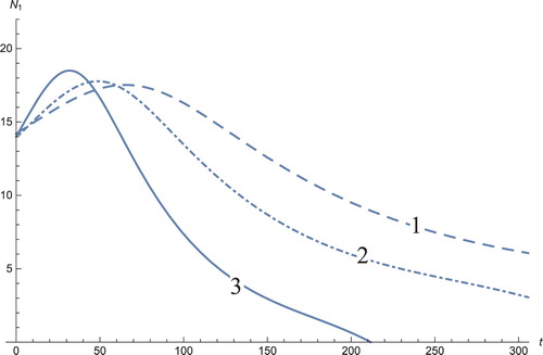
Figure 2. The solution profiles of $N_2\left(t\right)$, the androgen-independent cancer cells. 1: MDDIM, 2: QSS, quasi-steady state approximation, 3: numerical simulations for the full model. These cells decrease rapidly with the onset of immunotherapy.

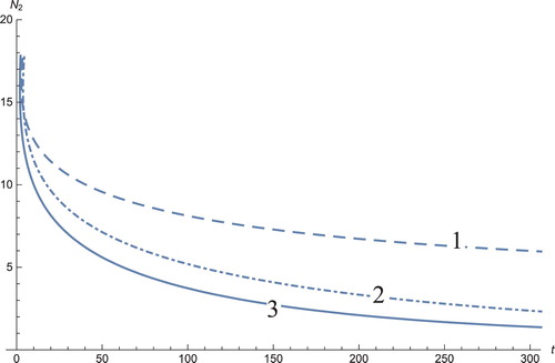
Figure 3. The solutions profiles of the T cells. 1: MDDIM, 2: QSS, quasi-steady state approximation, 3: numerical simulations for the full model. At first treatment, there is a very sharp increase in these cells and then drop to equilibrium point.

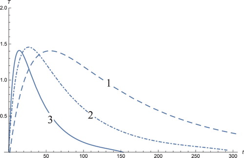
Figure 4. The solution profiles of $I_L\left(t\right)$, the concentration of cytokine. 1: MDDIM, 2: QSS, quasi-steady state approximation, 3: numerical simulations for the full model. During the treatment, the concentration of cytokines increases due to the intense activity of the immune system.

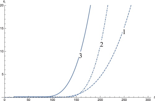
Figure 5. The solution profiles of $A\left(t\right)$, the concentration of androgen. 1: MDDIM, 2: QSS, quasi-steady state approximation, 3: numerical simulations for the full model. The androgens corresponding to the dendritic cells stabilize after ≈60 days, to their equilibrium point.

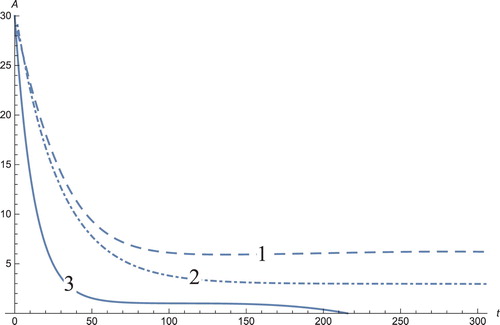
Figure 6. The solution profiles of D, the number of dendritic cells. 1: MDDIM, 2: QSS, quasi-steady state approximation, 3: numerical simulations for the full model. The number of dendritic cells stabilizes after $\approx 56$ days.

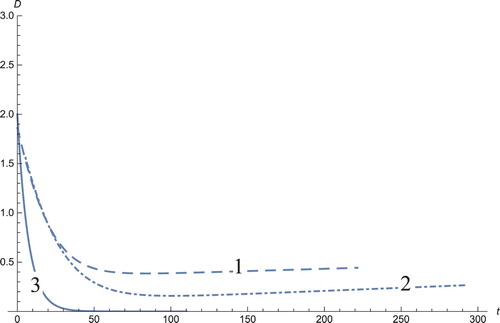
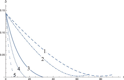
Figure 7. The solution profiles of ${\tilde{N}}_1$, the new variable in the new coordinates. 1: MDDIM, 2: QSS, quasi-steady state approximation, 3: numerical simulations for the full model in the new coordinates, 4: combination of MDDIM and SPVF, 5: SPVF method.

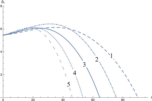
Figure 8. The solution profiles of ${\tilde{N}}_2$, the new variable in the new coordinates. 1: MDDIM, 2: QSS, quasi-steady state approximation, 3: numerical simulations for the full model in the new coordinates, 4: combination of MDDIM and SPVF, 5: SPVF method.

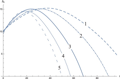
Figure 9. The solution profiles of $\tilde{T}$, the new variable in the new coordinates. 1: MDDIM, 2: QSS, quasi-steady state approximation, 3: numerical simulations for the full model in the new coordinates, 4: combination of MDDIM and SPVF, 5: SPVF method.

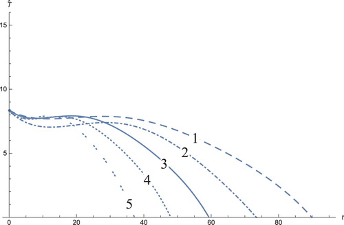
Figure 10. The solution profiles of ${\tilde{I}}_L$, the new variable in the new coordinates. 1: MDDIM, 2: QSS, quasi-steady state approximation, 3: numerical simulations for the full model in the new coordinates, 4: combination of MDDIM and SPVF, 5: SPVF method.

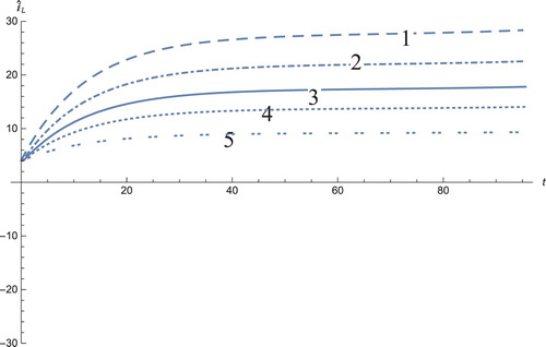
Figure 11. The solution profiles of $\tilde{A}$, the new variable in the new coordinates. 1: MDDIM, 2: QSS, quasi-steady state approximation, 3: numerical simulations for the full model in the new coordinates, 4: combination of MDDIM and SPVF, 5: SPVF method. Since we transfer the model using eigenvectors, we obtain a negative value of $\tilde{A}$ which is biologically insignificant. And hence, for sake of biological understanding, we must ignore these negative values.

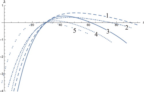
Figure 12. The solution profiles of $\tilde{D}$, the new variable in the new coordinates. 1: MDDIM, 2: QSS, quasi-steady state approximation, 3: numerical simulations for the full model in the new coordinates, 4: combination of MDDIM and SPVF, 5: SPVF method.

According to the results described by the figures presented herein, it is clear that the androgen-dependent cancer cells at the beginning of the treatment starting with the initial condition point increase up to $\approx 18\left[\mathrm{cells}\right]$, and subsequently decrease to zero (Figure 1). Furthermore, the T cells exhibit the same mathematical behaviour (Figure 3). The androgen-independent cancer cells begin at the initial condition of the system and decreases directly to zero without increasing (Figure 2). The concentration of cytokine increases exponentially and quickly. This result is practical from the biological point of view, because cytokines are secreted by the immune system, and immunotherapy actually stimulates the immune system as well as by other cells (Figure 4).

The graph showing the concentration of the androgens (Figure 5) shows a decrease in androgens and is a positive aspect, because the aim is to reduce the androgen that stimulates cancerous growths. The usual aggressive treatments for the reduction in androgen are orchiectomy (also named orchidectomy, and sometimes shortened as orchi), androgen blocker receptors, and androgen blockers in the thyroid gland (the adrenal glands (also known as suprarenal glands)), blocks the production of gonadotropin-releasing hormones (GnRH or LHRH) such as LH from the hypothalamus. Most cancer cells lose their sensitivity to hormone therapy after several years. In this study, the androgens decrease to zero through immunotherapy for the graph obtained by numerical simulations and stabilize for the system solution using the MDDIM and QSS methods. The number of DCs (Figure 6) decreases, coherent to the androgen decrease.

The solution profiles of the model presented in the new coordinates are unnecessary. The graphs do not provide additional information and biological insights beyond what that presented and analysed above. However, the presentation of these graphs presents mathematical importance, in that when the system is presented in the new coordinates, the resulting graphs are indeed a linear combination of the model solutions in the old coordinates with the corresponding coefficients (Figures 7–12)

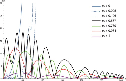
Figure 13 presents the PSA concentration level for the different cases of the controlled parameter $e_1$. When the value of this parameter is small, the level of PSA increases exponentially; when the value of this parameter increases, the level of PSA decreases. This implies that the treatment lengths vary between patients depending on the value of $e_1$. If we increase $e_1$, subsequently the length of ‘ of-treatment’ is much longer, resulting in more comfort for the patient.

Figure 13. PSA serum level, with an injection rate of 0.078 billion cells for various values of $e_1$, the maximum rate T cells kill cancer cells. A wider range of $e_1$ is able to suppress the growth of cancer and elongate the cycles of IAD.

5. Conclusion

In this research, we presented the mathematical model of evolution and treatment of prostate cancer. The treatment was performed using the immune system to attack the cancer cells. Our analysis included the effect of DC vaccines on the long-term behaviour of prostate cancer. This treatment improved the life quality of the patients and may delay the resistance toward treatment. Immunotherapy altered the body immune system to help fight this type of cancer. The mathematical model included a system of nonlinear ODEs of the first order and described the interaction between androgen-dependent cancer cells, androgen-independent cancer cells, activated T cells, concentration of cytokine, concentration of androgen and number of DCs. Because the system was complex and comprised a hidden hierarchy, we applied the SPVF method to expose this hierarchy. After implementing the SPVF algorithm, we applied different asymptotical methods because the system decomposed into fast and slow subsystems. In this study, we combined two semi-asymptotical–analytical methods called the SPVF and MDDIM methods to investigate the progression of the cancer cells. In addition, our analysis included a comparison between different methods for solving the system (described the interaction between the treatment and the cancer cells). The comparison involved the implementation of our new method (the combination of MDDIM and SPVF), MDDIM, SPVF, solving the full model numerically using the Runge–Kutta simulation and QSS approximation. In addition, we investigated the stability of the system around its equilibrium points.

In general, after applying the SPVF method, i.e. transferring the system of the governing equations to new coordinates and exposing the small parameters of the system, the system exhibited the same form as that assumed in the QSS approximation. Therefore, the question emerged as to why the SPVF method must be applied, To apply the QSS approximation, the system should be in the form of an SPS, i.e. a system with explicit separation to fast and slow subsystems, thereby implying that the system should contain explicitly small parameters. Otherwise, one should assume, based on intuition or the experimental results, which dynamical variables of the system change fast and which change slow. In the presented model, we assumed that the androgen, cytokines and DCs change slowly compared to the other variables of the system. This assumption was reasonable because the time scales at which these processes occurred were much shorter than that of the populations of growing cancer cells. In contrast to the QSS method, the SPVF method could be applied to any system without the initial conditions regarding the variables of the system, as well as without transferring the system to the SPS form. The SPVF method revealed that the fast direction of the system was a combination of the ‘old’ variables of the system such that the cancer cells changed (grew) slowly and decreased to zero. After we applied the SPVF method that only transferred the model to new coordinates, we applied the MDDIM method that is a semi-analytical method to obtain the solution profiles of the system. Our results, in comparison with others, indicated that the optimal interaction of immunotherapy was the interaction described by the fast direction of the system with the appropriate coefficients. Nevertheless, the treatment should be adapted to the patient and other parameters should be considered for different patients. For example, the parameter $e_1$ could be a patient-specific parameter, as it is the maximum rate that T cells kill cancer cells per day. These parameters were controlled by the therapist; for patients with weaker immune systems, more frequent injections (appropriate combination between these parameters) could be much more effective. Similarly, the amount of DCs could be controlled by changing Equation (9(9) $\frac{\mathrm{d}D}{\mathrm{d}t}=\underset{\mathrm{natural}\mathrm{death}}{\underbrace{-cD}}\equiv F_6\left(\overrightarrow{V}\right),$(9) ), for example, to the form of $\left(\mathrm{d}D/\mathrm{d}t\right)=\delta -cD$ where δ is the injection rate.

Disclosure statement

No potential conflict of interest was reported by the authors.

References

- P.A. Abrahamsson, Intermittent androgen deprivation therapy in patients with prostate cancer: Connecting the dots, Asian J. Urol. 4 (2017), pp. 208–222. doi: 10.1016/j.ajur.2017.04.001
- American Cancer Society, Prostate Cancer, available at http://www.cancer.org.
- V. Bykov, I. Goldfarb and V. Gol'dshtein, Singularly perturbed vector fields, J. Phys. Conf. Ser. 55 (2006), pp. 28–44. doi: 10.1088/1742-6596/55/1/003
- V. Bykov and U. Maas, Reaction–diffusion manifolds and global quasi-linearization: Two complementary methods for mechanism reduction, Open Thermodyn. J. 7 (2013), pp. 92–100.
- G. Dimonte, A cell kinetics model for prostate cancer and its application to clinical data and individual patients, J. Theor. Biol. 264 (2010), pp. 420–442. doi: 10.1016/j.jtbi.2010.02.023
- S.E. Eikenberry, J.D. Nagy and Y. Kuang, The evolutionary impact of androgen levels on prostate cancer in a multi-scale mathematical model, Biol. Dir. 5 (2010), pp. 24. doi: 10.1186/1745-6150-5-24
- Q. Guo, Y. Tao and K. Aihara, Mathematical modelling of prostate tumor growth under intermittent androgen suppression with partial differential equations, Int. J. Bifurcat. Chaos Appl. Sci. Eng. 18 (2008), pp. 3789–3797. doi: 10.1142/S0218127408022743
- A.M. Ideta, G. Tanaka, T. Takeuchi and A. Kazuyuki, A mathematical model of intermittent androgen suppression for prostate cancer, J. Nonlin. Sci. 18 (2008), pp. 593–614. doi: 10.1007/s00332-008-9031-0
- T.L. Jackson, A mathematical investigation of the multiple pathways to recurrent prostate cancer: Comparison with experimental data, Neoplasia 6 (2004), pp. 679–704. doi: 10.1593/neo.04259
- T.L. Jackson, A mathematical model of prostate tumor growth and androgen-independent relapse, Discrete Contin. Dyn. Sys. Ser. B (2004), pp. 187–201.
- H.V. Jain, S.K. Clinton, A. Bhinder and A. Friedman, Mathematical modeling of prostate cancer progression in response to androgen ablation therapy, PNAS Proc. Nat. Acad. Sci. USA. 108 (2011), pp. 19701–19706. doi: 10.1073/pnas.1115750108
- D. Kirschner and J.C. Panetta, Modeling immunotherapy of the tumor–immune interaction, J. Math. Biol. 37(3) (1998), pp. 235–252. doi: 10.1007/s002850050127
- N. Kronik, Y. Kogan, M. Elishmereni, K.H. Tobias, S.V. Pavlovic and Z. Agur, Predicting outcomes of prostate cancer immunotherapy by Personalized Mathematical Models, PLoS One 5(12) (2010), pp. 1–8. doi: 10.1371/journal.pone.0015482
- S.J. Liao, The proposed homotopy analysis technique for the solution of nonlinear problems, PhD thesis, Shanghai Jiao Tong University, 1992.
- S.J. Liao, Homotopy analysis method in nonlinear differential equations, Springer, China Press, 2000.
- S.J. Liao, Beyond perturbation: Introduction to the homotopy analysis method, Chapman & Hall/CRC Press, Boca Raton, 2003.
- S.J. Liao and Y. Zhao, On the method of directly defining inverse mapping for nonlinear differential equations, Numer. Algor. 72(4) (2016), pp. 989–1020. doi: 10.1007/s11075-015-0077-4
- N. Mottet, J. Bellmunt, E. Briers, R.C.N. van den Bergh, M. Bolla, N.J. van Casteren, P. Cornford, S. Culine, S. Joniau, T. Lam, M.D. Mason, V. Matveev, H. van der Poel, T.H. Vanderkwast, O. Rouvire and T. Wiegel, European Association of Urology (EAU) Prostate Cancer Guidelines, available at http://uroweb.org/2015.
- T. Osada, T.M. Clay, C.Y. Woo, M.A. Morse and H.K. Lyerly, Dendritic cell-based immunotherapy, Int. Rev. Immunol. 25(56) (2006), pp. 377–413. doi: 10.1080/08830180600992456
- T. Portz, Y. Kuang and J.D. Nagy, A clinical data validated mathematical model of prostate cancer growth under intermittent androgen suppression therapy, Amer. Inst. Phys. 2 (2012), pp. 1–14.
- E.M. Rutter and Y. Kuang, Global dynamics of a model of joint hormone treatment with dendritic cell vaccine for prostate cancer, DCDS-B 22 (2017), pp. 1001–1021. doi: 10.3934/dcdsb.2017050
- R.L. Sabado, S. Balan and N. Bhardwaj, Dendritic cell-based immunotherapy, Cell Res. Nat. 27 (2017), pp. 74–95. doi: 10.1038/cr.2016.157
- T. Shimada and K. Aihara, A nonlinear model with competition between prostate tumor cells and its application to intermittent androgen suppression therapy of prostate cancer, Math. Biosci. 214 (2008), pp. 134–139. doi: 10.1016/j.mbs.2008.03.001
- Y. Tao, Q. Guo and K. Aihara, A model at the macroscopic scale of prostate tumor growth under intermittent androgen suppression, Math. Models Methods Appl. Sci. 19 (2009), pp. 2177–2201. doi: 10.1142/S021820250900408X
- Y. Tao, Q. Guo and K. Aihara, A mathematical model of prostate tumor growth under hormone therapy with mutation inhibitor, J. Non. Sci. 20 (2010), pp. 219–240. doi: 10.1007/s00332-009-9056-z
- P. Travis and K. Yang, A mathematical model for the immunotherapy of advanced cancer, Proceedings: International Symposium on Mathematical and Computational Biology, September 2, 2012 14:40.