A delayed HIV infection model with apoptosis and viral loss

ABSTRACT

In this paper, a delayed human immunodeficiency virus (HIV) model with apoptosis of cells has been studied. Both immunological and intracellular delay have been incorporated to make the model more relevant. Firstly, the model has been investigated using local stability analysis. Next, the global stability analysis of steady states has been performed. The stability switch criteria taking the delay as the bifurcating parameter, leading to Hopf bifurcation has been studied. The transition of the system from order to chaos has been explored, and the analytical results have been verified by numerical simulations. The results thus can be used to describe the extensive dynamics exhibited by the model introduced in this article. The effects of apoptosis on viral load has been studied in the model numerically.

KEYWORDS:

• Apoptosis
• chaos
• global stability
• HIV
• Hopf bifurcation
• time delay
• viral loss

AMS CLASSIFICATIONS:

• 34K18
• 34K20
• 34K60
• 93A30
• 92C50

1. Introduction

Human immunodeficiency virus (HIV) emerged in the 1980s, and since then it has affected a large number of world population. HIV is the causative agent of acquired immunodeficiency syndrome (AIDS). HIV viruses are parasites which strive on Langerhans, macrophages, dendritic cells and CD4+ T cells. The virus is initially controlled by the immune response comprising of the cytotoxic T lymphocytes (CTLs) and the B cell antibodies [7,26,27]. In most patients infected with HIV, the viral load remains at low levels for years. This stage is called as the period of clinical latency. The plasma virus RNA is detectable, the generation and destruction rates of the virus are very high. However, for reasons not discovered yet, a discontinuity in this control, results in a remarkable decrease in the number of CD4+ T cells, along with a quick rise in the viral level. This decrease marks the end of the clinical latency period, and the person is said to have progressed to AIDS [6,37]. The three primary ways which lead to low level of CD4+ T cells in the body can be listed as the viral contamination of cells, the effect of apoptosis on the infected cells and the removal of contaminated cells by CTLs [9].

Mathematical modelling has contributed to a considerable extent in decoding the dynamics of HIV infection. The models have focused on various interactions between different components of HIV infection. The initial models classified the infection dynamics as interactions among the uninfected T cells, infected T cells and the virus [2,5,16,30,31]. The incorporation of the immune response in the models provided a greater understanding of the dynamics of HIV infection [19,23,26]. A major shortcoming of the previous models was the ignorance of the effect of delays on the system. Herz et al. [15] introduced a model of HIV infection with intracellular delay. Intracellular delay can be defined as the time lapse between the entry of the virus to viral production. Various other models have been proposed since then [18,35,41,43,44,49]. The delay in the activation of immune response is called immunological delay. This delay has been considered in several papers [29,44,47,48]. The combined effect of these delays has been discussed by only a few authors [1,28,29,39,45]. Using multiple delays in the model provides a better understanding of the system. However, these models pose a greater challenge in their analysis because the resulting models bear highly complex and non-linear equations.

The major anti-viral drugs for treating HIV are reverse transcriptase inhibitor (RTI) and protease inhibitor (PI). RTI hinders reverse transcriptase and hence inhibits transformation of viral RNA to DNA. Protease Inhibitor negates viral duplication, and hence, viral multiplication stays suppressed. Combination therapy called highly active anti-retro-viral therapy (HAART) includes treatment with both these drugs. The combined treatment together is more efficient on the HIV and restricts the viral load at the lowest level. With the advancement of drug therapy, the researchers are now focused on developing models with drug therapy [11,24,32–34,40].

The uninfected cell loss in HIV infection exceeds the infected cell population. One of the major causes for this difference in the number of cells is the increased destruction of the uninfected T cells [6]. In HIV infection, the increase in the destruction of T cells can arise by direct toxicity of infected cells or apoptosis in uninfected T cells also known as bystander cells. This is triggered by soluble membrane-bound viral factors [17]. Apoptosis can thus, be defined as programmed cell death. Bystander apoptosis is the lysis of uninfected bystander T cells. Gougeon et al. [10] showed a correlation between apoptosis and disease progression, implying that HIV kills the cell it infects. It has also been concluded that viral markers associate with T cells, and activate an apoptotic signal which results in the lysis of the uninfected T cells [20]. The exclusion of the effect of bystander apoptosis on the count of CD4+ T cells is a major shortcoming of the previous studies. Guo and Ma [12] introduced a model based on Bystander apoptosis and studied its global behaviour. Fan et al. [8] proposed a mathematical model which included the activation-induced apoptosis phenomenon and examined the effect of apoptosis on viral infection dynamics, with special emphasis on HIV.

It has been argued that loss of the virus is minuscule and can be included in the virus removal term [38]. However, Heffernan et al. [13,14] concluded that this loss has a significant role in determining the covariance between helper T cells and viral load. Wang et al. [46] in their paper have concluded that viral waning term affects the reproduction number as well as the infected equilibrium points, thus affecting the overall viral dynamics of the system.

Based on the discussion above, in this article, we propose to discuss the model proposed by Sahani et al. [36], which involves the growth of uninfected T cells, the growth of viruses, CTL immune response, the intracellular delay, the immunological delay along with combination drug therapy. The proposed model is thus a delayed model and has been analysed using local stability theory, bifurcation theory and Lyapunov stability theory. This paper is organized as follows. In Section 2 the model has been discussed followed by a discussion of the basic properties of the model in Section 3. In Section 4 the equilibrium states and threshold dynamics of the system have been analysed along with a discussion of the local stability of the model. Global stability analysis has been discussed in Section 5. The numerical simulation has been analysed in Section 6 followed by conclusions and discussion in Section 7.

2. Mathematical model

In this article, a four dimensional delayed model which includes combination therapy, apoptosis of the T cells and loss of virus cells as described in Sahani et al. [36] is assumed as follows: (1) $\begin{array}{r}\begin{array}{rl}{x}_1^{\prime }\left(t\right)& =s-\mathrm{d}{x}_1\left(t\right)-b(1-{ϵ}_r)x_1\left(t\right)x_3\left(t\right)\\ & -\frac{k{x}_1\left(t\right)x_3\left(t\right)}{x_1\left(t\right)+B},\\ x_2^{\prime }\left(t\right)& =b(1-{ϵ}_r)x_1(t-{\tau }_1)x_3(t-{\tau }_1)\\ & -\delta x_2\left(t\right)-d_1{x}_4\left(t\right)x_2\left(t\right),\\ x_3^{\prime }\left(t\right)& =N\delta (1-{ϵ}_p)x_2\left(t\right)-c{x}_3\left(t\right)\\ & -\eta b{x}_3\left(t\right)x_1\left(t\right),\\ x_4^{\prime }\left(t\right)& =p{x}_2(t-{\tau }_2)x_4(t-{\tau }_2)-d_2{x}_4\left(t\right).\end{array}\end{array}$(1) Here $x_1$, $x_2$, $x_3$ and $x_4$ represents uninfected T cells, infected T cells, viruses and CTL immune response cells respectively. The parameters ${\tau }_1$ and ${\tau }_2$ are intracellular delay and immunological delay respectively. The definition of the various parameters have been described in Table 1.

Table 1. Descriptions of various parameters.

Parameters	Their descriptions
s	Production rate of uninfected T cells
d	Death rate of uninfected T cells
b	Rate of infection of T cells by virus
${ϵ}_r$	Efficacy of RTI
k	Removal rate of uninfected T cells
B	Bystander apoptosis
δ	Death rate of infected T cells
$d_1$	Rate of action of CTL cells
N	Lysis rate of infected cells
${ϵ}_p$	Efficacy of PI
c	Death rate of virus
η	Loss of virus
p	Production rate of CTL cells
$d_2$	Death rate of CTL cells

The initial conditions of system (1(1) $\begin{array}{r}\begin{array}{rl}{x}_1^{\prime }\left(t\right)& =s-\mathrm{d}{x}_1\left(t\right)-b(1-{ϵ}_r)x_1\left(t\right)x_3\left(t\right)\\ & -\frac{k{x}_1\left(t\right)x_3\left(t\right)}{x_1\left(t\right)+B},\\ x_2^{\prime }\left(t\right)& =b(1-{ϵ}_r)x_1(t-{\tau }_1)x_3(t-{\tau }_1)\\ & -\delta x_2\left(t\right)-d_1{x}_4\left(t\right)x_2\left(t\right),\\ x_3^{\prime }\left(t\right)& =N\delta (1-{ϵ}_p)x_2\left(t\right)-c{x}_3\left(t\right)\\ & -\eta b{x}_3\left(t\right)x_1\left(t\right),\\ x_4^{\prime }\left(t\right)& =p{x}_2(t-{\tau }_2)x_4(t-{\tau }_2)-d_2{x}_4\left(t\right).\end{array}\end{array}$(1) ) are defined as follows: (2) $\begin{array}{r}\begin{array}{rl}{x}_1\left(\theta \right)& ={\xi }_1\left(\theta \right),x_2\left(\theta \right)={\xi }_2\left(\theta \right),\\ x_3\left(\theta \right)& ={\xi }_3\left(\theta \right),x_4\left(\theta \right)={\xi }_4\left(\theta \right),\end{array}\end{array}$(2) where $\xi =({\xi }_1,{\xi }_2,{\xi }_3,{\xi }_4)\in C\left(\right[-\tau ,0],R_{+}^4)$ where C is the Banach space of all continuous functions mapping from $[-\tau ,0]$ into $R_{+}^4$, $\tau =max\{{\tau }_1,{\tau }_2\}$ and $\theta \in [-\tau ,0]$. Moreover, functions ${\xi }_i$ satisfies the conditions ${\xi }_i\left(0\right)>0$ so that the system (1(1) $\begin{array}{r}\begin{array}{rl}{x}_1^{\prime }\left(t\right)& =s-\mathrm{d}{x}_1\left(t\right)-b(1-{ϵ}_r)x_1\left(t\right)x_3\left(t\right)\\ & -\frac{k{x}_1\left(t\right)x_3\left(t\right)}{x_1\left(t\right)+B},\\ x_2^{\prime }\left(t\right)& =b(1-{ϵ}_r)x_1(t-{\tau }_1)x_3(t-{\tau }_1)\\ & -\delta x_2\left(t\right)-d_1{x}_4\left(t\right)x_2\left(t\right),\\ x_3^{\prime }\left(t\right)& =N\delta (1-{ϵ}_p)x_2\left(t\right)-c{x}_3\left(t\right)\\ & -\eta b{x}_3\left(t\right)x_1\left(t\right),\\ x_4^{\prime }\left(t\right)& =p{x}_2(t-{\tau }_2)x_4(t-{\tau }_2)-d_2{x}_4\left(t\right).\end{array}\end{array}$(1) ) always permits non-negative solutions. Theorem 3.2 in the following section gives positive invariance and boundedness of the solutions in positive orthant.

3. Basic properties of model

We use the following well known lemma to prove the existence and uniqueness of positive solution of the system (1(1) $\begin{array}{r}\begin{array}{rl}{x}_1^{\prime }\left(t\right)& =s-\mathrm{d}{x}_1\left(t\right)-b(1-{ϵ}_r)x_1\left(t\right)x_3\left(t\right)\\ & -\frac{k{x}_1\left(t\right)x_3\left(t\right)}{x_1\left(t\right)+B},\\ x_2^{\prime }\left(t\right)& =b(1-{ϵ}_r)x_1(t-{\tau }_1)x_3(t-{\tau }_1)\\ & -\delta x_2\left(t\right)-d_1{x}_4\left(t\right)x_2\left(t\right),\\ x_3^{\prime }\left(t\right)& =N\delta (1-{ϵ}_p)x_2\left(t\right)-c{x}_3\left(t\right)\\ & -\eta b{x}_3\left(t\right)x_1\left(t\right),\\ x_4^{\prime }\left(t\right)& =p{x}_2(t-{\tau }_2)x_4(t-{\tau }_2)-d_2{x}_4\left(t\right).\end{array}\end{array}$(1) ).

Lemma 3.1

Assume that for the following system of differential equations in ${\mathbb{R}}^n$ with ${\mathbb{R}}_{+}^n=[0,\mathrm{\infty }{)}^n$ defined as (3) $\begin{array}{r}\begin{array}{rl}\frac{\mathrm{d}X\left(t\right)}{\mathrm{d}t}& =F(t,X(t\left)\right),\\ X\left(0\right)& =X_0\in {\mathbb{R}}_{+}^n,\end{array}\end{array}$(3) and $F_j(t,X){|}_{X_j=0}\ge 0$ whenever choosing $X\in {\mathbb{R}}_{+}^n$ such that $X_j=0$. Then, the system (1(1) $\begin{array}{r}\begin{array}{rl}{x}_1^{\prime }\left(t\right)& =s-\mathrm{d}{x}_1\left(t\right)-b(1-{ϵ}_r)x_1\left(t\right)x_3\left(t\right)\\ & -\frac{k{x}_1\left(t\right)x_3\left(t\right)}{x_1\left(t\right)+B},\\ x_2^{\prime }\left(t\right)& =b(1-{ϵ}_r)x_1(t-{\tau }_1)x_3(t-{\tau }_1)\\ & -\delta x_2\left(t\right)-d_1{x}_4\left(t\right)x_2\left(t\right),\\ x_3^{\prime }\left(t\right)& =N\delta (1-{ϵ}_p)x_2\left(t\right)-c{x}_3\left(t\right)\\ & -\eta b{x}_3\left(t\right)x_1\left(t\right),\\ x_4^{\prime }\left(t\right)& =p{x}_2(t-{\tau }_2)x_4(t-{\tau }_2)-d_2{x}_4\left(t\right).\end{array}\end{array}$(1) ) will have a unique non-negative solution provided F is locally Lipschitz [42].

Theorem 3.2

Let $\left(x_1\right(t),x_2(t),x_3(t),x_4(t\left)\right)$ be the solution of the system (1(1) $\begin{array}{r}\begin{array}{rl}{x}_1^{\prime }\left(t\right)& =s-\mathrm{d}{x}_1\left(t\right)-b(1-{ϵ}_r)x_1\left(t\right)x_3\left(t\right)\\ & -\frac{k{x}_1\left(t\right)x_3\left(t\right)}{x_1\left(t\right)+B},\\ x_2^{\prime }\left(t\right)& =b(1-{ϵ}_r)x_1(t-{\tau }_1)x_3(t-{\tau }_1)\\ & -\delta x_2\left(t\right)-d_1{x}_4\left(t\right)x_2\left(t\right),\\ x_3^{\prime }\left(t\right)& =N\delta (1-{ϵ}_p)x_2\left(t\right)-c{x}_3\left(t\right)\\ & -\eta b{x}_3\left(t\right)x_1\left(t\right),\\ x_4^{\prime }\left(t\right)& =p{x}_2(t-{\tau }_2)x_4(t-{\tau }_2)-d_2{x}_4\left(t\right).\end{array}\end{array}$(1) ) with initial conditions given by Equation (2(2) $\begin{array}{r}\begin{array}{rl}{x}_1\left(\theta \right)& ={\xi }_1\left(\theta \right),x_2\left(\theta \right)={\xi }_2\left(\theta \right),\\ x_3\left(\theta \right)& ={\xi }_3\left(\theta \right),x_4\left(\theta \right)={\xi }_4\left(\theta \right),\end{array}\end{array}$(2) ). Then $x_1\left(t\right)>0,x_2\left(t\right)>0,x_3\left(t\right)>0,x_4\left(t\right)>0$ are ultimately bounded.

Proof.

It is obvious that the right-hand side function $G(t,X(t\left)\right)$ of system (1(1) $\begin{array}{r}\begin{array}{rl}{x}_1^{\prime }\left(t\right)& =s-\mathrm{d}{x}_1\left(t\right)-b(1-{ϵ}_r)x_1\left(t\right)x_3\left(t\right)\\ & -\frac{k{x}_1\left(t\right)x_3\left(t\right)}{x_1\left(t\right)+B},\\ x_2^{\prime }\left(t\right)& =b(1-{ϵ}_r)x_1(t-{\tau }_1)x_3(t-{\tau }_1)\\ & -\delta x_2\left(t\right)-d_1{x}_4\left(t\right)x_2\left(t\right),\\ x_3^{\prime }\left(t\right)& =N\delta (1-{ϵ}_p)x_2\left(t\right)-c{x}_3\left(t\right)\\ & -\eta b{x}_3\left(t\right)x_1\left(t\right),\\ x_4^{\prime }\left(t\right)& =p{x}_2(t-{\tau }_2)x_4(t-{\tau }_2)-d_2{x}_4\left(t\right).\end{array}\end{array}$(1) ) is locally Lipschitz and therefore there exist a unique solution for a given initial condition. To prove the positivity of the solutions of system (1(1) $\begin{array}{r}\begin{array}{rl}{x}_1^{\prime }\left(t\right)& =s-\mathrm{d}{x}_1\left(t\right)-b(1-{ϵ}_r)x_1\left(t\right)x_3\left(t\right)\\ & -\frac{k{x}_1\left(t\right)x_3\left(t\right)}{x_1\left(t\right)+B},\\ x_2^{\prime }\left(t\right)& =b(1-{ϵ}_r)x_1(t-{\tau }_1)x_3(t-{\tau }_1)\\ & -\delta x_2\left(t\right)-d_1{x}_4\left(t\right)x_2\left(t\right),\\ x_3^{\prime }\left(t\right)& =N\delta (1-{ϵ}_p)x_2\left(t\right)-c{x}_3\left(t\right)\\ & -\eta b{x}_3\left(t\right)x_1\left(t\right),\\ x_4^{\prime }\left(t\right)& =p{x}_2(t-{\tau }_2)x_4(t-{\tau }_2)-d_2{x}_4\left(t\right).\end{array}\end{array}$(1) ), we first prove the positivity over the interval $[0,\tau ]$, and then repeat the process over $[\tau ,2\tau ]$ and so on. Thus, generalizing the result over any finite interval $[0,t]$. Considering the right-hand side functions of equations of the system (1(1) $\begin{array}{r}\begin{array}{rl}{x}_1^{\prime }\left(t\right)& =s-\mathrm{d}{x}_1\left(t\right)-b(1-{ϵ}_r)x_1\left(t\right)x_3\left(t\right)\\ & -\frac{k{x}_1\left(t\right)x_3\left(t\right)}{x_1\left(t\right)+B},\\ x_2^{\prime }\left(t\right)& =b(1-{ϵ}_r)x_1(t-{\tau }_1)x_3(t-{\tau }_1)\\ & -\delta x_2\left(t\right)-d_1{x}_4\left(t\right)x_2\left(t\right),\\ x_3^{\prime }\left(t\right)& =N\delta (1-{ϵ}_p)x_2\left(t\right)-c{x}_3\left(t\right)\\ & -\eta b{x}_3\left(t\right)x_1\left(t\right),\\ x_4^{\prime }\left(t\right)& =p{x}_2(t-{\tau }_2)x_4(t-{\tau }_2)-d_2{x}_4\left(t\right).\end{array}\end{array}$(1) ) over the time interval $[0,\tau ]$, we observe that $\begin{array}{rl}G(t,X(t\left)\right)& ={\left[\begin{array}{c}{G}_1(t,X(t\left)\right)\\ G_2(t,X(t\left)\right)\\ G_3(t,X(t\left)\right)\\ G_4(t,X(t\left)\right)\end{array}\right]}_{X_j\left(t\right)=0}\\ & =\left[\begin{array}{c}s\\ b(1-{ϵ}_r)x_1(t-{\tau }_1)x_3(t-{\tau }_1)\\ (1-{ϵ}_p)N\delta x_2\\ p{x}_2(t-{\tau }_2)x_4(t-{\tau }_2)\end{array}\right]\\ & =\left[\begin{array}{c}s\\ b(1-{ϵ}_r){\xi }_1\left(\theta \right){\xi }_3\left(\theta \right)\\ (1-{ϵ}_p)N\delta x_2\\ p{\xi }_2\left(\theta \right){\xi }_4\left(\theta \right)\end{array}\right],\end{array}$ where $\theta \in [-\tau ,0]$. It can be seen from the above expression that each components $G_j(t,X(t\left)\right)\ge 0$ whenever $X_j=0$ and $X\in {\mathbb{R}}_{+}^n$ because parameters takes all positive values and initial functions are also non-negative. Therefore, solutions of system (1(1) $\begin{array}{r}\begin{array}{rl}{x}_1^{\prime }\left(t\right)& =s-\mathrm{d}{x}_1\left(t\right)-b(1-{ϵ}_r)x_1\left(t\right)x_3\left(t\right)\\ & -\frac{k{x}_1\left(t\right)x_3\left(t\right)}{x_1\left(t\right)+B},\\ x_2^{\prime }\left(t\right)& =b(1-{ϵ}_r)x_1(t-{\tau }_1)x_3(t-{\tau }_1)\\ & -\delta x_2\left(t\right)-d_1{x}_4\left(t\right)x_2\left(t\right),\\ x_3^{\prime }\left(t\right)& =N\delta (1-{ϵ}_p)x_2\left(t\right)-c{x}_3\left(t\right)\\ & -\eta b{x}_3\left(t\right)x_1\left(t\right),\\ x_4^{\prime }\left(t\right)& =p{x}_2(t-{\tau }_2)x_4(t-{\tau }_2)-d_2{x}_4\left(t\right).\end{array}\end{array}$(1) ) remain non-negative in $[0,\tau ]$. Similarly, in the interval $[\tau ,2\tau ]$, $\begin{array}{rl}G(t,X(t\left)\right)& ={\left[\begin{array}{c}{G}_1(t,X(t\left)\right)\\ G_2(t,X(t\left)\right)\\ G_3(t,X(t\left)\right)\\ G_4(t,X(t\left)\right)\end{array}\right]}_{X_j\left(t\right)=0}\\ & =\left[\begin{array}{c}s\\ b(1-{ϵ}_r)x_1(t-{\tau }_1)x_3(t-{\tau }_1)\\ (1-{ϵ}_p)N\delta x_2\\ p{x}_2(t-{\tau }_2)x_4(t-{\tau }_2)\end{array}\right]\\ & =\left[\begin{array}{c}s\\ b(1-{ϵ}_r)x_1\left(\phi \right)x_3\left(\phi \right)\\ (1-{ϵ}_p)N\delta x_2\\ p{x}_2\left(\phi \right)x_4\left(\phi \right)\end{array}\right],\end{array}$ and $\phi \in [0,\tau ]$. With similar arguments as in above case, solutions of system (1(1) $\begin{array}{r}\begin{array}{rl}{x}_1^{\prime }\left(t\right)& =s-\mathrm{d}{x}_1\left(t\right)-b(1-{ϵ}_r)x_1\left(t\right)x_3\left(t\right)\\ & -\frac{k{x}_1\left(t\right)x_3\left(t\right)}{x_1\left(t\right)+B},\\ x_2^{\prime }\left(t\right)& =b(1-{ϵ}_r)x_1(t-{\tau }_1)x_3(t-{\tau }_1)\\ & -\delta x_2\left(t\right)-d_1{x}_4\left(t\right)x_2\left(t\right),\\ x_3^{\prime }\left(t\right)& =N\delta (1-{ϵ}_p)x_2\left(t\right)-c{x}_3\left(t\right)\\ & -\eta b{x}_3\left(t\right)x_1\left(t\right),\\ x_4^{\prime }\left(t\right)& =p{x}_2(t-{\tau }_2)x_4(t-{\tau }_2)-d_2{x}_4\left(t\right).\end{array}\end{array}$(1) ) remain non-negative in $[\tau ,2\tau ]$ also. Continuing in this way, it can be easily proved that for any finite interval $[0,t]$, the solutions of the system (1(1) $\begin{array}{r}\begin{array}{rl}{x}_1^{\prime }\left(t\right)& =s-\mathrm{d}{x}_1\left(t\right)-b(1-{ϵ}_r)x_1\left(t\right)x_3\left(t\right)\\ & -\frac{k{x}_1\left(t\right)x_3\left(t\right)}{x_1\left(t\right)+B},\\ x_2^{\prime }\left(t\right)& =b(1-{ϵ}_r)x_1(t-{\tau }_1)x_3(t-{\tau }_1)\\ & -\delta x_2\left(t\right)-d_1{x}_4\left(t\right)x_2\left(t\right),\\ x_3^{\prime }\left(t\right)& =N\delta (1-{ϵ}_p)x_2\left(t\right)-c{x}_3\left(t\right)\\ & -\eta b{x}_3\left(t\right)x_1\left(t\right),\\ x_4^{\prime }\left(t\right)& =p{x}_2(t-{\tau }_2)x_4(t-{\tau }_2)-d_2{x}_4\left(t\right).\end{array}\end{array}$(1) ) remain non-negative.

To prove the boundedness of the solutions, we have first considered the first equation of system (1(1) $\begin{array}{r}\begin{array}{rl}{x}_1^{\prime }\left(t\right)& =s-\mathrm{d}{x}_1\left(t\right)-b(1-{ϵ}_r)x_1\left(t\right)x_3\left(t\right)\\ & -\frac{k{x}_1\left(t\right)x_3\left(t\right)}{x_1\left(t\right)+B},\\ x_2^{\prime }\left(t\right)& =b(1-{ϵ}_r)x_1(t-{\tau }_1)x_3(t-{\tau }_1)\\ & -\delta x_2\left(t\right)-d_1{x}_4\left(t\right)x_2\left(t\right),\\ x_3^{\prime }\left(t\right)& =N\delta (1-{ϵ}_p)x_2\left(t\right)-c{x}_3\left(t\right)\\ & -\eta b{x}_3\left(t\right)x_1\left(t\right),\\ x_4^{\prime }\left(t\right)& =p{x}_2(t-{\tau }_2)x_4(t-{\tau }_2)-d_2{x}_4\left(t\right).\end{array}\end{array}$(1) ) which implies $\frac{\mathrm{d}{x}_1}{\mathrm{d}t}\le s-\mathrm{d}{x}_1\left(t\right).$ Thus, $lim\underset{t\to \mathrm{\infty }}{sup}{x}_1\left(t\right)\le s/d$ and so $x_1$ is bounded. Now consider the function $X_1$ defined as follows: $X_1\left(t\right)=x_1\left(t\right)+x_2(t+{\tau }_1).$ Clearly, $X_1\left(t\right)\ge 0$ for all $t\ge 0$. Taking the derivative of $X_1$ along solutions of model (1(1) $\begin{array}{r}\begin{array}{rl}{x}_1^{\prime }\left(t\right)& =s-\mathrm{d}{x}_1\left(t\right)-b(1-{ϵ}_r)x_1\left(t\right)x_3\left(t\right)\\ & -\frac{k{x}_1\left(t\right)x_3\left(t\right)}{x_1\left(t\right)+B},\\ x_2^{\prime }\left(t\right)& =b(1-{ϵ}_r)x_1(t-{\tau }_1)x_3(t-{\tau }_1)\\ & -\delta x_2\left(t\right)-d_1{x}_4\left(t\right)x_2\left(t\right),\\ x_3^{\prime }\left(t\right)& =N\delta (1-{ϵ}_p)x_2\left(t\right)-c{x}_3\left(t\right)\\ & -\eta b{x}_3\left(t\right)x_1\left(t\right),\\ x_4^{\prime }\left(t\right)& =p{x}_2(t-{\tau }_2)x_4(t-{\tau }_2)-d_2{x}_4\left(t\right).\end{array}\end{array}$(1) ) gives $\begin{array}{rl}\frac{\mathrm{d}{X}_1}{\mathrm{d}t}& \le s-\mathrm{d}{x}_1\left(t\right)-\delta x_2(t+{\tau }_1)\\ & \le s-Q_{1}X.\end{array}$ Thus, $lim\underset{t\to \mathrm{\infty }}{sup}{X}_1\left(t\right)\le s/Q_1$ where $Q_1=min\{d,\delta \}$ and so $x_2$ is bounded by an $M_1>0$. Again, in order to prove that $x_3$ is bounded, consider the third equation of model (1(1) $\begin{array}{r}\begin{array}{rl}{x}_1^{\prime }\left(t\right)& =s-\mathrm{d}{x}_1\left(t\right)-b(1-{ϵ}_r)x_1\left(t\right)x_3\left(t\right)\\ & -\frac{k{x}_1\left(t\right)x_3\left(t\right)}{x_1\left(t\right)+B},\\ x_2^{\prime }\left(t\right)& =b(1-{ϵ}_r)x_1(t-{\tau }_1)x_3(t-{\tau }_1)\\ & -\delta x_2\left(t\right)-d_1{x}_4\left(t\right)x_2\left(t\right),\\ x_3^{\prime }\left(t\right)& =N\delta (1-{ϵ}_p)x_2\left(t\right)-c{x}_3\left(t\right)\\ & -\eta b{x}_3\left(t\right)x_1\left(t\right),\\ x_4^{\prime }\left(t\right)& =p{x}_2(t-{\tau }_2)x_4(t-{\tau }_2)-d_2{x}_4\left(t\right).\end{array}\end{array}$(1) ) which gives $\frac{\mathrm{d}{x}_3}{\mathrm{d}t}\le N\delta (1-{ϵ}_p)x_2\left(t\right)-c{x}_3\left(t\right).$ Therefore, $lim\underset{t\to \mathrm{\infty }}{sup}{x}_3\left(t\right)\le N\delta M_1(1-{ϵ}_p)/c=Q_2$ and so $x_3$ is bounded by an $M_2>0$. Lastly, to prove that $x_4$ is also bounded, consider the function $X_2$ as follows: $X_2\left(t\right)=x_2\left(t\right)+\frac{d_1}{p}{x}_4(t+{\tau }_2).$ It is obvious that $X_2\left(t\right)\ge 0$ for all $t\ge 0$ as $x_2$ and $x_4$ are non-negative. Now, taking derivative of $X_2$ along solutions of model (1(1) $\begin{array}{r}\begin{array}{rl}{x}_1^{\prime }\left(t\right)& =s-\mathrm{d}{x}_1\left(t\right)-b(1-{ϵ}_r)x_1\left(t\right)x_3\left(t\right)\\ & -\frac{k{x}_1\left(t\right)x_3\left(t\right)}{x_1\left(t\right)+B},\\ x_2^{\prime }\left(t\right)& =b(1-{ϵ}_r)x_1(t-{\tau }_1)x_3(t-{\tau }_1)\\ & -\delta x_2\left(t\right)-d_1{x}_4\left(t\right)x_2\left(t\right),\\ x_3^{\prime }\left(t\right)& =N\delta (1-{ϵ}_p)x_2\left(t\right)-c{x}_3\left(t\right)\\ & -\eta b{x}_3\left(t\right)x_1\left(t\right),\\ x_4^{\prime }\left(t\right)& =p{x}_2(t-{\tau }_2)x_4(t-{\tau }_2)-d_2{x}_4\left(t\right).\end{array}\end{array}$(1) ) gives $\begin{array}{rl}\frac{\mathrm{d}{X}_2}{\mathrm{d}t}& \le \frac{bs{M}_2(1-{ϵ}_r)}{d}-\delta x_2\left(t\right)-\frac{d_1{d}_2}{p}{x}_4(t+{\tau }_2)\\ & =\frac{bs{M}_2(1-{ϵ}_r)}{d}-Q_3{X}_2\left(t\right).\end{array}$ Thus, it is clear that $lim\underset{t\to \mathrm{\infty }}{sup}{X}_2\left(t\right)\le bs{M}_2(1-{ϵ}_r)/d{Q}_3$ where $Q_3=min\{\delta ,d_2\}$ and hence $x_4$ is bounded by an $M_3>0$.

4. Local dynamics of steady states

There are three types of steady states of the system namely the infection free state $I_0$, infected state $I_1$ and the immune response absent steady state $I_2$ are respectively given by $\begin{array}{rl}{I}_0& =(x_1^0,0,0,0)=\left(\frac{s}{d},0,0,0\right),\\ I_1& =(x_1^{\ast },x_2^{\ast },x_3^{\ast },x_4^{\ast }),\\ I_2& =(x_1^{\prime },x_2^{\prime },x_3^{\prime },x_4^{\prime }),\end{array}$ where $\begin{array}{rl}{x}_2^{\ast }& =\frac{d_2}{p},\\ x_3^{\ast }& =\frac{N\delta d_2(1-{ϵ}_p)}{p(c+b{x}_1^{\ast }\eta )},\\ x_4^{\ast }& =\frac{x_1^{\ast }\left(bN\delta \right(1-{ϵ}_r\left)\right(1-{ϵ}_p)-b\delta \eta )-c\delta }{d_1(c+b{x}_1^{\ast }\eta )}.\end{array}$ The coordinate $x_1^{\ast }$ of the infected steady state $I_1$ can be determined from the cubic equation ${\alpha }_0{x}_1^{\ast 3}+{\alpha }_1{x}_1^{\ast 2}+{\alpha }_2{x}_1^{\ast }+{\alpha }_3=0,$ with coefficients given by $\begin{array}{rl}{\alpha }_0& =bdp\eta ,\\ {\alpha }_1& =cdp+bBdp\eta -bps\eta +bN\delta d_2(1-{ϵ}_p)(1-{ϵ}_r),\\ {\alpha }_2& =Bcdp-cps-bBps\eta +kN\delta d_2(1-{ϵ}_p)\\ & +bBN\delta d_2(1-{ϵ}_p)(1-{ϵ}_r),\\ {\alpha }_3& =-Bcps.\end{array}$ The coordinates of $I_2$ are given by $\begin{array}{rl}{x}_1^{\prime }& =\frac{c}{bN(1-{ϵ}_r)(1-{ϵ}_p)-k\eta },x_3^{\prime }=\frac{x_2^{\prime }\delta \left(bN\right(1-{ϵ}_r\left)\right(1-{ϵ}_p)-k\eta )}{bc(1-{ϵ}_r)},x_4^{\prime }=0,\\ x_2^{\prime }& =\frac{\begin{array}{c}b(1-{ϵ}_r)\left(bNs\right(1-{ϵ}_r\left)\right(1-{ϵ}_p)-cd-\eta ks)\\ (-bBN(1-{ϵ}_r\left)\right(1-{ϵ}_p)+B\eta k-c)\end{array}}{\begin{array}{c}\delta \left(bN\right(1-{ϵ}_r\left)\right(1-{ϵ}_p)-\eta k)bN(1-{ϵ}_r)(1-{ϵ}_p)\\ \left(bB\right(1-{ϵ}_r)+k)-bB\eta k(1-{ϵ}_r)+bc(1-{ϵ}_r)-\eta k^2\end{array}}.\end{array}$ In order to state the threshold dynamics of infection-free equilibrium state, it is necessary to define the basic reproduction number of the model. The basic reproduction number of the model can be defined as $R_0=\frac{s\left(bN\right(1-{ϵ}_r\left)\right(1-{ϵ}_p)-b\eta )}{cd}.$ In this paper we are interested in analysing the effect of immune response after HIV infection. Hence, the analysis has been performed only for the infection-free and infected equilibrium.

4.1. Stability analysis of $I_1$

The first step in the analytical study of a model is its local stability analysis. So, in this section, the stability of the infected steady state $I_1$ has been discussed. The stability analysis of the infection-free steady state $I_0$ can be easily proved and has been discussed in paper [36]. Therefore, the following theorem is stated without proof for the stability of infection-free equilibrium point $I_0$.

Theorem 4.1

If $R_0<1$ then infection-free equilibrium $I_0$ is locally asymptotically stable and unstable if $R_0>1$.

To study the stability behaviour of $I_1$, the characteristic equation of system (1(1) $\begin{array}{r}\begin{array}{rl}{x}_1^{\prime }\left(t\right)& =s-\mathrm{d}{x}_1\left(t\right)-b(1-{ϵ}_r)x_1\left(t\right)x_3\left(t\right)\\ & -\frac{k{x}_1\left(t\right)x_3\left(t\right)}{x_1\left(t\right)+B},\\ x_2^{\prime }\left(t\right)& =b(1-{ϵ}_r)x_1(t-{\tau }_1)x_3(t-{\tau }_1)\\ & -\delta x_2\left(t\right)-d_1{x}_4\left(t\right)x_2\left(t\right),\\ x_3^{\prime }\left(t\right)& =N\delta (1-{ϵ}_p)x_2\left(t\right)-c{x}_3\left(t\right)\\ & -\eta b{x}_3\left(t\right)x_1\left(t\right),\\ x_4^{\prime }\left(t\right)& =p{x}_2(t-{\tau }_2)x_4(t-{\tau }_2)-d_2{x}_4\left(t\right).\end{array}\end{array}$(1) ) at the infected equilibrium is considered which is (4) $\begin{array}{rl}& P\left(\lambda \right)+e^{-\lambda {\tau }_2}Q\left(\lambda \right)+e^{-\lambda {\tau }_1}R\left(\lambda \right)\\ & +e^{-\lambda ({\tau }_2+{\tau }_1)}S\left(\lambda \right)=0,\end{array}$(4) where the polynomials P, Q, R and S are given by (5) $\begin{array}{r}\begin{array}{rl}P\left(\lambda \right)& ={\lambda }^4+p_3{\lambda }^3+p_2{\lambda }^2+p_1\lambda +p_0,\\ Q\left(\lambda \right)& =q_3{\lambda }^3+q_2{\lambda }^2+q_1\lambda +q_0,\\ R\left(\lambda \right)& =r_2{\lambda }^2+r_1\lambda +r_0,\\ S\left(\lambda \right)& =s_1\lambda +s_0.\end{array}\end{array}$(5) The coefficients appearing in above polynomial are determined by the following set of relations: $\begin{array}{rl}{p}_3& =a_{11}+a_{22}+a_{33}+a_{44},\\ p_2& =(a_{11}+a_{44})(a_{22}+a_{33})+a_{44}{a}_{11}+a_{22}{a}_{33}-a_{13}{a}_{31},\\ p_1& =a_{22}{a}_{44}(a_{11}+a_{33})+(a_{22}+a_{44})(a_{11}{a}_{33}-a_{13}{a}_{31}),\\ p_0& =a_{22}{a}_{44}(-a_{13}{a}_{31}+a_{11}{a}_{33}),\\ q_3& =-a_{44},\\ q_2& =a_{24}{a}_{42}-a_{44}(a_{11}+a_{22}+a_{33}),\\ q_1& =a_{24}{a}_{42}(a_{11}+a_{33})-a_{44}{a}_{11}(a_{22}+a_{33})\\ & +a_{44}(a_{13}{a}_{31}-a_{22}{a}_{33}),\\ q_0& =a_{42}{a}_{24}(-a_{13}{a}_{31}+a_{11}{a}_{33})\\ & +a_{44}{a}_{22}(a_{13}{a}_{31}-a_{11}{a}_{33}),\\ r_2& =a_{23}{a}_{32},\\ r_1& =a_{32}(a_{13}{a}_{21}-a_{23}(a_{11}+a_{44}\left)\right),\\ r_0& =-a_{44}{a}_{32}(a_{13}{a}_{21}+a_{11}{a}_{23}),\\ s_1& =a_{23}{a}_{32}{a}_{44},\\ s_0& =a_{44}{a}_{32}(a_{11}{a}_{23}+a_{13}{a}_{21}).\end{array}$ $\begin{array}{rl}{ϵ}_r^{\prime }& =1-{ϵ}_r,{ϵ}_p^{\prime }=1-{ϵ}_p,\\ a_{11}& =d+\frac{Bk{x}_3^{\ast }}{(B+x_1^{\ast }{)}^2}+b{x}_3^{\ast }{ϵ}_r^{\prime },\\ a_{13}& =\frac{k{x}_1^{\ast }}{(B+x_1^{\ast })}+b{x}_1^{\ast }{ϵ}_r^{\prime },\\ a_{21}& =-b{x}_3^{\ast }{ϵ}_r^{\prime },a_{22}=\delta +x_4^{\ast }{d}_1,\\ a_{23}& =b{x}_1^{\ast }{ϵ}_r^{\prime },a_{24}=\frac{d_1{d}_2}{p},\\ a_{31}& =b\eta x_3^{\ast },a_{32}=N{ϵ}_p^{\prime }\delta ,\\ a_{33}& =c+b{x}_1^{\ast }\eta ,a_{42}=p{x}_4^{\ast },\\ a_{44}& =d_2.\end{array}$ The local stability of equilibrium points $I_1$ with ${\tau }_1={\tau }_2=0$ and ${\tau }_1\ne 0,{\tau }_2=0$ can be determined from the following set of Theorems 4.2–4.4, the proof or explanation for which can be found in Sahani et al. [36].

Theorem 4.2

Let $R_0>1$ and ${\tau }_1={\tau }_2=0,$ in this case Equation (4(4) $\begin{array}{rl}& P\left(\lambda \right)+e^{-\lambda {\tau }_2}Q\left(\lambda \right)+e^{-\lambda {\tau }_1}R\left(\lambda \right)\\ & +e^{-\lambda ({\tau }_2+{\tau }_1)}S\left(\lambda \right)=0,\end{array}$(4) ) reduces to (6) $\begin{array}{rl}& {\lambda }^4+(p_3+q_3){\lambda }^3+(p_2+q_2+r_2){\lambda }^2\\ & +(p_1+q_1+r_1+s_1)\lambda \\ & +p_0+q_0+r_0+s_0=0,\end{array}$(6) and $I_1$ is locally asymptotically stable if $H1\left(a\right)$–$\left(c\right)$ holds, where

1. $(p_3+q_3)>0$, $(p_2+q_2+r_2)>0$,

2. $(p_1+q_1+r_1+s_1)>0$, $(p_0+q_0+r_0+s_0)>0$,

3. $(p_3+q_3)(p_2+q_2+r_2)-(p_1+q_1+r_1+s_1)>0$,

4. $(p_3+q_3)(p_2+q_2+r_2)(p_1+q_1+r_1+s_1)-(p_3+q_3{)}^2(p_0+q_0+r_0+s_0)-(p_1+q_1+r_1+s_1{)}^2>0.$

The above theorem gives the stability conditions when both delays vanish but when ${\tau }_2=0$ and ${\tau }_1\ne 0$, even then the equilibrium point can be stable for all values of ${\tau }_1$. The required conditions can be summarized in the following Theorem.

Theorem 4.3

Let $R_0>1$ with ${\tau }_2=0$ and ${\tau }_1\ne 0,$ Equation (4(4) $\begin{array}{rl}& P\left(\lambda \right)+e^{-\lambda {\tau }_2}Q\left(\lambda \right)+e^{-\lambda {\tau }_1}R\left(\lambda \right)\\ & +e^{-\lambda ({\tau }_2+{\tau }_1)}S\left(\lambda \right)=0,\end{array}$(4) ) reduces to (7) $\begin{array}{rl}& {\lambda }^4+(p_3+q_3){\lambda }^3+(p_2+q_2){\lambda }^2+(p_1+q_1)\lambda +p_0+q_0\\ & +e^{-\lambda {\tau }_1}\left(r_2{\lambda }^2+(r_1+s_1)\lambda +r_0+s_0\right)=0,\end{array}$(7) and $I_1$ is locally asymptotically stable for all values of ${\tau }_1$ if $H1\left(a\right)$–$\left(c\right)$ and $H2\left(a\right)$–$\left(c\right)$ holds, where

1. $\left(\right(p_3+q_3{)}^2-2(p_2+q_2))>0$,

2. $\left(\right(p_2+q_2+r-2\left)\right(p_2+q_2-r_2)-(2p_1+q_1\left)\right(q_3+p_3)+2(p_0+q_0\left)\right)>0,$ $\left(\right(p_1+q_1+r_1+s_1\left)\right(p_1+q_1-r_1-s_1)-2(p_2+q_2\left)\right(p_0+q_0)+2r_2(r_0+s_0\left)\right)>0,$

3. $(p_0+q_0-r_0-s_0)>0$.

There exists another conditions under which the equilibrium point $I_1$ can be stable for certain interval of ${\tau }_1$ i.e. in $[0,{\tau }_1^{\ast }]$. In general if this happens, the system is then stable for so many such interval such as $[{\tau }_{1_{2m}},{\tau }_{1_{2m+1}}]$. To facilitate this discussion, assuming $\lambda =\mathrm{i}\omega$ in Equation (7(7) $\begin{array}{rl}& {\lambda }^4+(p_3+q_3){\lambda }^3+(p_2+q_2){\lambda }^2+(p_1+q_1)\lambda +p_0+q_0\\ & +e^{-\lambda {\tau }_1}\left(r_2{\lambda }^2+(r_1+s_1)\lambda +r_0+s_0\right)=0,\end{array}$(7) ) gives the following equation: $\begin{array}{rl}F\left(\omega \right)& ={\omega }^8+\left(\right(p_3+q_3{)}^2-2(p_2+q_2)){\omega }^6\\ & +\left(\right(p_2+q_2+r_2\left)\right(p_2+q_2-r_2)\\ & -2(p_1+q_1)(q_3+p_3)+2(p_0+q_0)){\omega }^4\\ & +\left(\right(p_1+q_1+r_1+s_1\left)\right(p_1+q_1-r_1-s_1)\\ & -2(p_2+q_2)(p_0+q_0)+2r_2(r_0+s_0)){\omega }^2\\ & +(p_0+q_0+r_0+s_0)(p_0+q_0-r_0-s_0).\end{array}$ It is clear that if $(p_0+q_0-r_0-s_0)<0$ then equation $F\left(\omega \right)=0$ has a positive real roots. Corresponding to this positive roots ${\omega }_{1_i}$ of $F\left(\omega \right)=0$, the value of the delay ${\tau }_1$ can be given by (8) ${\tau }_{1_i}^{\left(n\right)}=\frac{1}{{\omega }_{1_i}}{\cos }^{-1}\left\{\frac{{△}_N}{{▽}_D}\right\}+\frac{2n\pi }{{\omega }_{1_i}}$(8) for i=1,2,3,4 and $n=0,1,2,3,\dots$ where $\begin{array}{rl}{△}_N& =(p_0+q_0)(r_0+s_0)-q_1(r_0+s_0){\omega }_{1_i}\\ & +\left((p_0+q_0)(-r_2+p_1(r_1+s_1\left)\right)\right.\\ & -\left.(p_2+q_2)(r_0+s_0)\right){\omega }_{1_i}^2\\ & +(q_1{r}_2+(p_3+q_3\left)\right(r_0+s_0\left)\right){\omega }_{1_i}^3\\ & +(r_0+s_0+(p_2+q_2\left)\right(r_2-p_1(r_1+s_1)){\omega }^4\\ & -r_2(p_3+q_3)){\omega }_{1_i}^5+(p_1(r_1+s_1)-r_2){\omega }_{1_i}^6,\\ {△}_D& =-(r_0+s_0{)}^2+2r_2(r_0+s_0){\omega }_{1_i}^2\\ & -p_1(r_1+s_1{)}^2{\omega }_{1_i}^3-r_2^2{\omega }_{1_i}^4.\end{array}$ The critical value of ${\tau }_1$ is then given by ${\tau }_1^{\ast }=min{\tau }_{1_i}^{\left(n\right)}.$ We now have the following theorem which states the stability switch criteria leading to the Hopf bifurcation in the system with respect to parameter ${\tau }_1$.

Theorem 4.4

Let $R_0>1,{\tau }_2=0,$ ${\tau }_1\ne 0,$ and $(p_0+q_0-r_0-s_0)<0$ holds, then there exits a critical value ${\tau }_1^{\ast }$ corresponding to ${\omega }_1^{\ast }$ such that the infected equilibrium $I_1$ is asymptotically stable in the interval $[0,{\tau }_1^{\ast })$. Further if $F^{\prime }\left(\right({\omega }_1^{\ast }{)}^2)\ne 0,$ then Hopf bifurcation is exhibited by system (1(1) $\begin{array}{r}\begin{array}{rl}{x}_1^{\prime }\left(t\right)& =s-\mathrm{d}{x}_1\left(t\right)-b(1-{ϵ}_r)x_1\left(t\right)x_3\left(t\right)\\ & -\frac{k{x}_1\left(t\right)x_3\left(t\right)}{x_1\left(t\right)+B},\\ x_2^{\prime }\left(t\right)& =b(1-{ϵ}_r)x_1(t-{\tau }_1)x_3(t-{\tau }_1)\\ & -\delta x_2\left(t\right)-d_1{x}_4\left(t\right)x_2\left(t\right),\\ x_3^{\prime }\left(t\right)& =N\delta (1-{ϵ}_p)x_2\left(t\right)-c{x}_3\left(t\right)\\ & -\eta b{x}_3\left(t\right)x_1\left(t\right),\\ x_4^{\prime }\left(t\right)& =p{x}_2(t-{\tau }_2)x_4(t-{\tau }_2)-d_2{x}_4\left(t\right).\end{array}\end{array}$(1) ) at the critical value ${\tau }_1^{\ast }$.

Since, as per the above discussion and theorems, interval of stability of the system $[0,{\tau }_1^{\ast })$ has been obtained, we vary the delay parameter ${\tau }_2$ in this interval to obtain the critical value ${\tau }_2^{\ast }$ to obtain the stability switch criteria. To obtain this, suppose $R_0>1$, ${\tau }_2\ne 0$ and ${\tau }_1={\tau }_{1_s}\in [0,{\tau }_1^{\ast })$, and let us treat ${\tau }_2$ as a bifurcation parameter. It is clear that $\lambda =0$ is not a root of Equation (4(4) $\begin{array}{rl}& P\left(\lambda \right)+e^{-\lambda {\tau }_2}Q\left(\lambda \right)+e^{-\lambda {\tau }_1}R\left(\lambda \right)\\ & +e^{-\lambda ({\tau }_2+{\tau }_1)}S\left(\lambda \right)=0,\end{array}$(4) ) as $p_0+q_0+r_0+s_0\ne 0$ and let $\lambda =\mathrm{i}\omega$ be a root of Equation (4(4) $\begin{array}{rl}& P\left(\lambda \right)+e^{-\lambda {\tau }_2}Q\left(\lambda \right)+e^{-\lambda {\tau }_1}R\left(\lambda \right)\\ & +e^{-\lambda ({\tau }_2+{\tau }_1)}S\left(\lambda \right)=0,\end{array}$(4) ). On substituting $\lambda =\mathrm{i}\omega$ in Equation (4(4) $\begin{array}{rl}& P\left(\lambda \right)+e^{-\lambda {\tau }_2}Q\left(\lambda \right)+e^{-\lambda {\tau }_1}R\left(\lambda \right)\\ & +e^{-\lambda ({\tau }_2+{\tau }_1)}S\left(\lambda \right)=0,\end{array}$(4) ) and separating real and imaginary parts gives the following two equation in ${\tau }_2$, (9) $\begin{array}{r}\begin{array}{rl}& C_1\cos \omega {\tau }_2+S_1\sin \omega {\tau }_2=p_0-p_2{\omega }^2+{\omega }^4\\ & +(r_0-r_2{\omega }^2)\cos \left(\omega {\tau }_{1_s}\right)+r_1\omega \sin \left(\omega {\tau }_{1_s}\right),\\ & C_2\cos \omega {\tau }_2+S_2\sin \omega {\tau }_2=p_1\omega -p_3{\omega }^3\\ & -(r_0-r_2{\omega }^2)\sin \left(\omega {\tau }_{1_s}\right)+r_1\omega \cos \left(\omega {\tau }_{1_s}\right)\end{array}\end{array}$(9) with $C_1$, $S_1$, $C_2$ and $S_2$ defined as follows: $\begin{array}{rl}{C}_1& =-q_0+q_2{\omega }^2-s_0\cos \omega {\tau }_{1_s}-s_1\omega \sin \omega {\tau }_{1_s},\\ S_1& =-q_1\omega +q_3{\omega }^3+s_0\sin \omega {\tau }_{1_s}-s_1\omega \cos \omega {\tau }_{1_s},\\ C_2& =-q_1\omega +q_3{\omega }^3+s_0\sin \omega {\tau }_{1_s}-s_1\omega \cos \omega {\tau }_{1_s},\\ S_2& =q_0-q_2{\omega }^2+s_0\cos \omega {\tau }_{1_s}+s_1\omega \sin \omega {\tau }_{1_s}.\end{array}$ On eliminating ${\tau }_2$ from the above two resulting equations gives (10) $\begin{array}{rl}K\left(\omega \right)& \equiv {\omega }^8+h_6{\omega }^6+h_5{\omega }^5+h_4{\omega }^4\\ & +h_3{\omega }^3+h_2{\omega }^2+h_1\omega +h_0=0,\end{array}$(10) where $\begin{array}{rl}{h}_6& =-2p_2+p_3^2-q_3^2-2r_2\cos \omega {\tau }_{1_s},\\ h_5& =2(r_1-p_3{r}_2)\sin \omega {\tau }_{1_s},\\ h_4& =2p_0+p_2^2-2p_1{p}_3-q_2^2+2q_1{q}_3+r_2^2\\ & +(2r_0-2p_3{r}_1+2p_2{r}_2-2s_1{q}_3)\cos \omega {\tau }_{1_s},\\ h_3& =(2p_3{r}_0-2p_2{r}_1+2p_1{r}_2-2r_0{q}_3+2q_2{s}_1)\sin \omega {\tau }_{1_s},\\ h_2& =p_1^2-2p_0{p}_2-q_1^2+2q_0{q}_2+r_1^2-2r_0{r}_2-s_1^2\\ & +2(p_1{r}_1-p_2{r}_0-p_0{r}_2+q_2{s}_0-q_1{s}_1)\cos \omega {\tau }_{1_s},\\ h_1& =2(-p_1{r}_0+p_0{r}_1+q_1{s}_0-q_0{s}_1)\sin \omega {\tau }_{1_s},\\ h_0& =p_0^2-q_0^2+r_0^2-s_0^2+(2p_0{r}_0-2q_0{s}_0)\cos \omega {\tau }_{1_s}.\end{array}$ FromEquation (10(10) $\begin{array}{rl}K\left(\omega \right)& \equiv {\omega }^8+h_6{\omega }^6+h_5{\omega }^5+h_4{\omega }^4\\ & +h_3{\omega }^3+h_2{\omega }^2+h_1\omega +h_0=0,\end{array}$(10) ), it is clear that $\underset{\omega \to \mathrm{\infty }}{lim}K\left(\omega \right)=\mathrm{\infty }$ and $K\left(0\right)=h_0=(p_0+q_0+r_0+s_0)(p_0+r_0-q_0-s_0).$ Now if $(p_0+r_0-q_0-s_0)<0$, then $K\left(0\right)<0$ and therefore Equation (10(10) $\begin{array}{rl}K\left(\omega \right)& \equiv {\omega }^8+h_6{\omega }^6+h_5{\omega }^5+h_4{\omega }^4\\ & +h_3{\omega }^3+h_2{\omega }^2+h_1\omega +h_0=0,\end{array}$(10) ) has at least one positive real root say ${\omega }_{2_j}$ j=1,2,3,4. Then from Equation (9(9) $\begin{array}{r}\begin{array}{rl}& C_1\cos \omega {\tau }_2+S_1\sin \omega {\tau }_2=p_0-p_2{\omega }^2+{\omega }^4\\ & +(r_0-r_2{\omega }^2)\cos \left(\omega {\tau }_{1_s}\right)+r_1\omega \sin \left(\omega {\tau }_{1_s}\right),\\ & C_2\cos \omega {\tau }_2+S_2\sin \omega {\tau }_2=p_1\omega -p_3{\omega }^3\\ & -(r_0-r_2{\omega }^2)\sin \left(\omega {\tau }_{1_s}\right)+r_1\omega \cos \left(\omega {\tau }_{1_s}\right)\end{array}\end{array}$(9) ), the value of ${\tau }_2$ is given by (11) ${\tau }_{2_j}^{\left(n\right)}=\frac{1}{{\omega }_{2_j}}{\cos }^{-1}\left(\frac{△}{▽}\right)+\frac{2n\pi }{{\omega }_{2_j}},$(11) for j=1,2,3,4, $n=0,1,2,3,\dots$ where $\begin{array}{rl}△& =a(p_0-p_2{\omega }_{2_j}^2+{\omega }_{2_j}^4)+b(p_1{\omega }_{2_j}-b{p}_3{\omega }_{2_j}^3)\\ & +(aA+bB)\cos {\omega }_{2_j}{\tau }_{1_s}+(aB-Ab)\sin {\omega }_{2_j}{\tau }_{1_s},\\ ▽& =a^2+b^2,\\ A& =(r_0-r_2{\omega }_{2_j}^2),\\ B& =r_1{\omega }_{2_j},\\ a& =q_2{\omega }_{2_j}^2-q_0-s_0\cos {\omega }_{2_j}{\tau }_{1_s}-s_1{\omega }_{2_j}\sin {\omega }_{2_j}{\tau }_{1_s},\\ b& =q_3{\omega }_{2_j}^3-q_1{\omega }_{2_j}+s_0\sin {\omega }_{2_j}{\tau }_{1_s}-s_1\cos {\omega }_{2_j}{\tau }_{1_s}.\end{array}$ The critical value ${\tau }_2^{\ast }$ of ${\tau }_2$ is given by taking the min of all the values of ${\tau }_2$ given by Equation (11(11) ${\tau }_{2_j}^{\left(n\right)}=\frac{1}{{\omega }_{2_j}}{\cos }^{-1}\left(\frac{△}{▽}\right)+\frac{2n\pi }{{\omega }_{2_j}},$(11) ) i.e. (12) ${\tau }_2^{\ast }=min{\tau }_{2_j}^{\left(n\right)}.$(12) Differentiating Equation (4(4) $\begin{array}{rl}& P\left(\lambda \right)+e^{-\lambda {\tau }_2}Q\left(\lambda \right)+e^{-\lambda {\tau }_1}R\left(\lambda \right)\\ & +e^{-\lambda ({\tau }_2+{\tau }_1)}S\left(\lambda \right)=0,\end{array}$(4) ) with respect to ${\tau }_2$ and rearranging similar term gives (13) ${\left(\frac{\mathrm{d}\lambda }{\mathrm{d}{\tau }_2}\right)}^{-1}=\frac{N_1}{D_1}-\frac{N_2}{D_2}-\frac{{\tau }_2}{\lambda },$(13) $\begin{array}{rl}{N}_1& =Q^{\prime }\left(\lambda \right)+e^{-\lambda {\tau }_{1_s}}{S}^{\prime }\left(\lambda \right)-{\tau }_{1_s}{e}^{-\lambda {\tau }_{1_s}}S\left(\lambda \right),\\ D_1& =\lambda \left(Q\right(\lambda )+e^{-\lambda {\tau }_{1_s}}S(\lambda \left)\right),\\ N_2& =P^{\prime }\left(\lambda \right)+e^{-\lambda {\tau }_{1_s}}\left(R^{\prime }\right(\lambda )-{\tau }_{1_s}R(\lambda \left)\right),\\ D_2& =\lambda \left(P\right(\lambda )+e^{-\lambda {\tau }_{1_s}}R(\lambda \left)\right).\end{array}$ The validation of transversability condition is an essential criteria for the occurrence of Hopf bifurcation. Hence, to study the shifting of real part of the eigenvalues from the negative to positive substitute, $\lambda \left({\tau }_2\right)=\mathrm{i}{\omega }_2^{\ast }$ in Equation (13(13) ${\left(\frac{\mathrm{d}\lambda }{\mathrm{d}{\tau }_2}\right)}^{-1}=\frac{N_1}{D_1}-\frac{N_2}{D_2}-\frac{{\tau }_2}{\lambda },$(13) ) and considering its real part gives $\begin{array}{rl}\text{sign}\left(\frac{\mathrm{d}\mathrm{\Re }\left(\lambda \right)}{\mathrm{d}{\tau }_2}{\mid }_{\lambda =\mathrm{i}{\omega }_2^{\ast }}\right)& =\text{sign}\left(\mathrm{\Re }{\left(\frac{\mathrm{d}\lambda }{\mathrm{d}{\tau }_2}\right)}^{-1}{\mid }_{\lambda =\mathrm{i}{\omega }_2^{\ast }}\right)\\ & =\text{sign}\left(\mathrm{\Re }\left[\frac{N_1}{D_1}-\frac{N_2}{D_2}\right]{\mid }_{\lambda =\mathrm{i}{\omega }_2^{\ast }}\right)\\ & =\text{sign}\left(\frac{K^{\prime }\left({\omega }_2^{\ast 2}\right)}{\chi }\right)\\ & =\text{sign}{K}^{\prime }\left({\omega }_2^{\ast 2}\right),\end{array}$ since $\chi =(Q+S\cos {\omega }_2^{\ast }{\tau }_{1_s}{)}^2+(S\sin {\omega }_2^{\ast }{\tau }_{1_s}{)}^2$ is always positive. Thus, considering all the informations and previous theorem, following theorem gives conditions for Hopf bifurcation.

Theorem 4.5

Let $R_0>1,$ ${\tau }_1\in [0,{\tau }_1^{\ast })$ and ${\tau }_2\ne 0$ then there exits a critical value ${\tau }_2^{\ast }$ and ${\omega }_2^{\ast }$ such that the infected equilibrium $I_1$ is asymptotically stable in the interval $[0,{\tau }_2^{\ast })$. Also if $(p_0+q_0-s_0-r_0)<0$ and $K^{\prime }\left(\right({\omega }_2^{\ast }{)}^2)\ne 0,$ then Hopf bifurcation is exhibited by system (1(1) $\begin{array}{r}\begin{array}{rl}{x}_1^{\prime }\left(t\right)& =s-\mathrm{d}{x}_1\left(t\right)-b(1-{ϵ}_r)x_1\left(t\right)x_3\left(t\right)\\ & -\frac{k{x}_1\left(t\right)x_3\left(t\right)}{x_1\left(t\right)+B},\\ x_2^{\prime }\left(t\right)& =b(1-{ϵ}_r)x_1(t-{\tau }_1)x_3(t-{\tau }_1)\\ & -\delta x_2\left(t\right)-d_1{x}_4\left(t\right)x_2\left(t\right),\\ x_3^{\prime }\left(t\right)& =N\delta (1-{ϵ}_p)x_2\left(t\right)-c{x}_3\left(t\right)\\ & -\eta b{x}_3\left(t\right)x_1\left(t\right),\\ x_4^{\prime }\left(t\right)& =p{x}_2(t-{\tau }_2)x_4(t-{\tau }_2)-d_2{x}_4\left(t\right).\end{array}\end{array}$(1) ) at the critical value ${\tau }_2^{\ast }$.

This completes the local stability and Hopf bifurcation analysis of model(1(1) $\begin{array}{r}\begin{array}{rl}{x}_1^{\prime }\left(t\right)& =s-\mathrm{d}{x}_1\left(t\right)-b(1-{ϵ}_r)x_1\left(t\right)x_3\left(t\right)\\ & -\frac{k{x}_1\left(t\right)x_3\left(t\right)}{x_1\left(t\right)+B},\\ x_2^{\prime }\left(t\right)& =b(1-{ϵ}_r)x_1(t-{\tau }_1)x_3(t-{\tau }_1)\\ & -\delta x_2\left(t\right)-d_1{x}_4\left(t\right)x_2\left(t\right),\\ x_3^{\prime }\left(t\right)& =N\delta (1-{ϵ}_p)x_2\left(t\right)-c{x}_3\left(t\right)\\ & -\eta b{x}_3\left(t\right)x_1\left(t\right),\\ x_4^{\prime }\left(t\right)& =p{x}_2(t-{\tau }_2)x_4(t-{\tau }_2)-d_2{x}_4\left(t\right).\end{array}\end{array}$(1) ). In the next section, we discuss the global behaviour of the equilibrium points of system(1(1) $\begin{array}{r}\begin{array}{rl}{x}_1^{\prime }\left(t\right)& =s-\mathrm{d}{x}_1\left(t\right)-b(1-{ϵ}_r)x_1\left(t\right)x_3\left(t\right)\\ & -\frac{k{x}_1\left(t\right)x_3\left(t\right)}{x_1\left(t\right)+B},\\ x_2^{\prime }\left(t\right)& =b(1-{ϵ}_r)x_1(t-{\tau }_1)x_3(t-{\tau }_1)\\ & -\delta x_2\left(t\right)-d_1{x}_4\left(t\right)x_2\left(t\right),\\ x_3^{\prime }\left(t\right)& =N\delta (1-{ϵ}_p)x_2\left(t\right)-c{x}_3\left(t\right)\\ & -\eta b{x}_3\left(t\right)x_1\left(t\right),\\ x_4^{\prime }\left(t\right)& =p{x}_2(t-{\tau }_2)x_4(t-{\tau }_2)-d_2{x}_4\left(t\right).\end{array}\end{array}$(1) ).

5. Global stability dynamics of steady states

In this section, the global stability of all equilibrium points is discussed. The LaSalle invariant principle and Lyapunov functional is used to arrive at the desired stability region for each equilibrium point.

Theorem 5.1

The infection-free equilibrium $I_0$ is globally asymptotically stable in the region D, where $D=\left\{(x_1,x_2,x_3,x_4):x_1\ge \frac{kbN{x}_1^0{ϵ}_p^{\prime }}{c-bN{x}_1^0{ϵ}_r^{\prime }{ϵ}_p^{\prime }}-B\right\},$ where ${ϵ}_p^{\prime }=1-{ϵ}_p,{ϵ}_r^{\prime }=1-{ϵ}_r,x_1^0=s/d$.

Proof.

To prove the global asymptotic stability of $I_0$, using Theorem 4.1 it is enough to prove it to be globally attractive. For this define the Lyapunov functional as $\begin{array}{rl}{V}_0\left(t\right)& =x_1^0\left(\frac{x_1}{x_1^0}-1-\ln \frac{x_1}{x_1^0}\right)+x_2+\frac{1}{N\delta {ϵ}_p^{\prime }}{x}_3+\frac{d_1}{p}{x}_4\\ & +b{ϵ}_r^{\prime }{\int }_{t-{\tau }_1}^t{x}_3\left(\xi \right)x_1\left(\xi \right)\mathrm{d}\xi \\ & +d_1{\int }_{t-{\tau }_2}^t{x}_2\left(\xi \right)x_4\left(\xi \right)\mathrm{d}\xi .\end{array}$ Differentiating the above function with respect to t gives $\begin{array}{rl}\dot{V_0}\left(t\right)& =-\frac{d}{x_1}(x_1-x_1^0{)}^2-\frac{k{x}_1{x}_3}{x_1+B}+b{x}_1^0{x}_3{ϵ}_r^{\prime }\\ & +\frac{k{x}_1^0{x}_3}{x_1+B}-\frac{c{x}_3}{N\delta {ϵ}_p^{\prime }}-\frac{\eta b{x}_1{x}_3}{N\delta {ϵ}_p^{\prime }}-\frac{d_1{d}_2{x}_4}{p}\\ & \le -\frac{d}{x_1}{\left(x_1-x_1^0\right)}^2\\ & +x_3\left(b{x}_1^0{ϵ}_p^{\prime }+\frac{k{x}_1^0}{x_1+B}-\frac{c}{N\delta {ϵ}_p^{\prime }}\right)\\ & \le 0\text{ in the defined domain }D\text{.}\end{array}$ Note that $\dot{V_0}\left(t\right)=0$ if and only if $x_1\left(t\right)=x_1^0\left(t\right),x_2\left(t\right)=x_3\left(t\right)=x_4\left(t\right)=0$. Thus the maximal compact invariant set for $\dot{V_0}\left(t\right)=0$ is $I_0$. So from LaSalle invariant principle, $I_0$ is globally attractive. Thus using Theorem 4.1 and the global attractiveness proved above, it can be concluded that $I_0$ is globally asymptotically stable in the domain D.

Theorem 5.2

The infected equilibrium $I_1$ is globally asymptotically stable in the region $D_1,$ where $\begin{array}{rl}{D}_1& =\left\{(x_1,x_2,x_3,x_4):\frac{kN{x}_1^{\ast }{ϵ}_p^{\prime }}{c-bN{ϵ}_r^{\prime }{ϵ}_p^{\prime }{x}_1^{\ast }}-B\le x_1\le x_1^{\ast }\right.\\ & \left.\mathrm{and}\frac{x_1^{\ast }{x}_3^{\ast }}{x_2^{\ast }}\le \frac{x_1{x}_3}{x_2}\le \frac{N{ϵ}_p^{\prime }}{c+\eta b{x}_1^{\ast }}\right\}\end{array}$

Proof.

Consider the function $H:R_{+}\to R_{+}$ defined by $H\left(x\right)=x-1-\ln x$ such that x=1 is the global minimum with $H\left(1\right)=0$. Then, to prove the global stability of the infected equilibrium $I_1$, define the Lyapunov functional $V_1$ as $\begin{array}{rl}{V}_1\left(t\right)& =x_1^{\ast }\left(\frac{x_1}{x_1^{\ast }}-1-\ln \frac{x_1}{x_1^{\ast }}\right)+x_2^{\ast }\left(\frac{x_2}{x_2^{\ast }}-1-\ln \frac{x_2}{x_2^{\ast }}\right)\\ & +x_3^{\ast }\left(\frac{x_3}{x_3^{\ast }}-1-\ln \frac{x_3}{x_3^{\ast }}\right)+\frac{d_1}{p}{x}_4\left(t\right)\\ & +{ϵ}_r^{\prime }b{x}_1^{\ast }{x}_3^{\ast }{\int }_{t-{\tau }_1}^{t}H\left(\frac{x_1\left(\xi \right)x_3\left(\xi \right)}{x_1^{\ast }{x}_3^{\ast }}\right)\mathrm{d}\xi \\ & +d_1{\int }_{t-{\tau }_2}^t{x}_2\left(\xi \right)x_4\left(\xi \right)\mathrm{d}\xi .\end{array}$ Differentiating the above equation with respect to t along the solution $I_1$ of system (1(1) $\begin{array}{r}\begin{array}{rl}{x}_1^{\prime }\left(t\right)& =s-\mathrm{d}{x}_1\left(t\right)-b(1-{ϵ}_r)x_1\left(t\right)x_3\left(t\right)\\ & -\frac{k{x}_1\left(t\right)x_3\left(t\right)}{x_1\left(t\right)+B},\\ x_2^{\prime }\left(t\right)& =b(1-{ϵ}_r)x_1(t-{\tau }_1)x_3(t-{\tau }_1)\\ & -\delta x_2\left(t\right)-d_1{x}_4\left(t\right)x_2\left(t\right),\\ x_3^{\prime }\left(t\right)& =N\delta (1-{ϵ}_p)x_2\left(t\right)-c{x}_3\left(t\right)\\ & -\eta b{x}_3\left(t\right)x_1\left(t\right),\\ x_4^{\prime }\left(t\right)& =p{x}_2(t-{\tau }_2)x_4(t-{\tau }_2)-d_2{x}_4\left(t\right).\end{array}\end{array}$(1) ) $\begin{array}{rl}\dot{V_1}\left(t\right)& =\left(1-\frac{x_1^{\ast }}{x_1}\right)\left(s-d{x}_1-b{ϵ}_r^{\prime }{x}_1{x}_3-\frac{k{x}_1{x}_3}{x_1+B}\right)\\ & +\left(1-\frac{x_2^{\ast }}{x_2}\right)\left(b{ϵ}_r^{\prime }x(t-{\tau }_1)x_3(t-{\tau }_1)\right.\\ & \left.-\delta x_2-d_1{x}_2{x}_4\right)\\ & +\left(1-\frac{x_3^{\ast }}{x_3}\right)\left(N{ϵ}_p^{\prime }\delta x_2-c{x}_3-\eta b{x}_1{x}_3\right)\\ & +\frac{d_1}{p}\left(p{x}_2(t-{\tau }_2)x_4(t-{\tau }_2)-d_2{x}_4\right)\\ & +{ϵ}_r^{\prime }b{x}_1^{\ast }{x}_3^{\ast }\left(\frac{x_1{x}_3}{x_1^{\ast }{x}_3^{\ast }}-\frac{x_1(t-{\tau }_1)x_3(t-{\tau }_1)}{x_1^{\ast }{x}_3^{\ast }}\right.\\ & \left.+\ln \frac{x_1(t-{\tau }_1)x_3(t-{\tau }_1)}{x_1{x}_3}\right)\\ & +d_1{x}_2{x}_4-d_1{x}_2(t-{\tau }_2)x_4(t-{\tau }_2).\end{array}$ On simplification, $\begin{array}{rl}\dot{V_1}\left(t\right)& \le -b{ϵ}_r^{\prime }{x}_1^{\ast }{x}_3^{\ast }\ln \frac{x_1{x}_2^{\ast }{x}_3}{x_1^{\ast }{x}_2{x}_3^{\ast }}+x_1^{\ast }\left[\frac{k{x}_3^{\ast }}{x_1^{\ast }+B}\right.\\ & \left.-\frac{k{x}_1^{\ast }{x}_3^{\ast }}{x_1(x_1^{\ast }+B)}-\frac{b{ϵ}_r^{\prime }{x}_1^{\ast }{x}_3^{\ast }}{x_1}+b{ϵ}_r^{\prime }{x}_3^{\ast }\right]\\ & +x_3\left[b{ϵ}_r^{\prime }{x}_1^{\ast }+\frac{k{x}_1^{\ast }}{x_1+B}-\frac{c}{N{ϵ}_p^{\prime }}\right]\\ & +x_3^{\ast }\left[\frac{c}{N{ϵ}_p^{\prime }}+\frac{\eta b{x}_1}{N{ϵ}_p^{\prime }}-\frac{\delta x_2}{x_3}\right]\\ & \le 0\text{ in the domain }{D}_1.\end{array}$ Also note that $\dot{V_1}\left(t\right)=0$ if and only if $x_1\left(t\right)=x_1^{\ast },x_2\left(t\right)=x_2^{\ast }\left(t\right),x_3\left(t\right)=x_3^{\ast }\left(t\right),x_4\left(t\right)=x_4^{\ast }\left(t\right)$. Thus the maximal compact invariant set $\dot{V_1}\left(t\right)=0$ is the singleton set $I_1$. So by using LaSalle invariant principle, the infected steady state $I_1$ is globally attractive.

6. Numerical simulation

In this section, we have performed numerical simulations to validate the theoretical results obtained in the previous sections and to give more insights into the long-term dynamics of the model. The data sets have mostly been taken from [3,4,21,22,25,31,46]. The effect of apoptosis on the viral load has been investigated using Data 1 given in Table 2 and the initial concentration of cells as $(800,0,1,0.001)$. It is evident from Figure 1 that as the rate of apoptosis increases, the first viral load peak increases but the time for achieving the viral peak value remains the same. It is also clear that the oscillations are sustained in the system, and an increase in apoptosis does not affect it. Thus, it can be concluded that an increase in the rate of apoptosis increases the viral load in the system.

Figure 1. Effect of apoptosis.

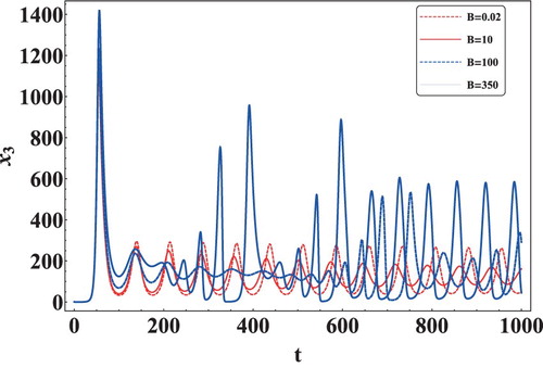
Table 2. The value of the various parameters.

Parameter	Data 1	Data 2	Data 3
s cells ml day^−1	46	5	200
d day^−1	0.0046	0.3	0.02
b ml viron day^−1	4.8$\times {10}^{-6}$	0.36	0.36
${ϵ}_r$	0.5	0.4	0.5
k cell^−1 day^−1	0.36	0.02	0.1
B day^−1	Varied	350	0.02
δ day^−1	0.1	0.33	0.53
$d_1$ ml viron day^−1	9.4$\times {10}^{-4}$	3.7$\times {10}^{-4}$	8.8
${ϵ}_p$	0.6	0.7	0.6
N virion cell^−1	4000	500	6167
c day^−1	3	3	3
η	20	20	19
p day^−1	0.46	1.4	0.4
$d_2$ day^−1	0.67	0.46	0.41
${\tau }_1$ days	0.09	11.5	0-5
${\tau }_2$ days	2	0.02	10-15

In Figure 2, by keeping the initial concentration of the cells same as above, we have plotted the graph of the uninfected T cell with single and combination therapy. It can be observed from Figure 2(a,b) that the combination therapy is more effective in increasing the T-cell count even with a lower efficacy drug as compared to a single drug therapy. In fact, as clear from these figures that the first T-cell peak in case of combination therapy is much higher than the case for single therapy drug. Thus combination therapy has more pronounced effect in increasing the healthy T-cell count in infected persons.

Figure 2. Comparison of single and combination therapy with black line showing single therapy and red line showing combination therapy.

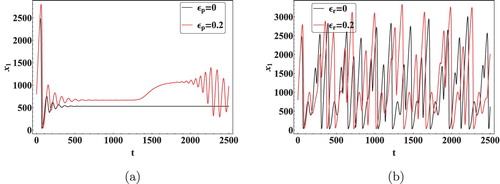
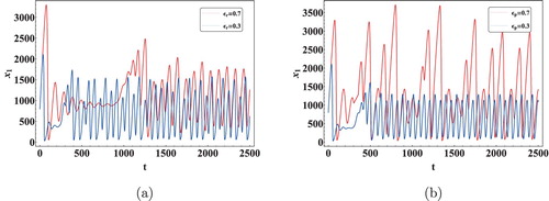
Next, we have used Data 1 and the same initial conditions as above, to highlight the effect of the drugs RTI and PI on the concentration of the uninfected T cells. From Figure 3(a), it is clear that there is a significant rise in the count of the uninfected T cells as the efficacy of RTI is increased from 0.3 to 0.7 keeping the effectiveness of PI fixed at 0.4. Next, RTI was set at 0.4, and the effectiveness of PI was changed from 0.3 to 0.7, in this case, it was observed that the increase in T-cell count was slightly more than the case when RTI was varied. From Figure 3(b) it was noted that the oscillations in the event of PI are more pronounced and the rise in the T-cell count was also greater than the case for RTI.

Figure 3. Effect of RTI and PI on the concentration of uninfected T cells (a) density of uninfected T cells for the different efficacy of PI keeping RTI fixed at 0.4, (b) density of uninfected T cells for the different efficacy of PI keeping RTI fixed at 0.4.

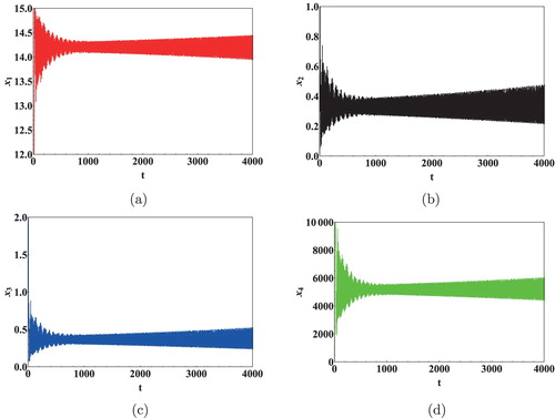
We next show the effect of time delays on the virus dynamics. Taking initial concentration of cells as $(10,0.01,1,0.001)$ and Data 2 from Table 2, we calculated the critical values of the delays. Keeping ${\tau }_2$ as 0, the critical value ${\tau }_1^{\ast }$ of ${\tau }_1$ was computed as 11.5 days [36]. It is clear from Figure 4 that $I_1$ is stable when ${\tau }_1<11.5$ and Hopf bifurcation occurs as ${\tau }_1$ crosses the critical valueFigure 5. Next as discussed in Theorem 4.5, let ${\tau }_1\in [0,11.5)$ and the critical value of ${\tau }_2$ was calculated to be 0.02 days. By using Theorem 4.5 it can be seen that as ${\tau }_2$ crosses the critical value the infected equilibrium $I_1$ becomes unstable, Hopf bifurcation can be seen in the system with the generation of periodic orbits as depicted in Figures 6 and 7. It is also interesting to note that a minuscule change in the immunological delay ${\tau }_2$ generates a significant shift in the dynamics of the system. Thus, it can be concluded that the immunological delay is more important than the intracellular delay in case of HIV infection.

Figure 4. Plots showing the asymptotic stability of the infected equilibrium $I_1$ when ${\tau }_1<{\tau }_1^{\ast }$.

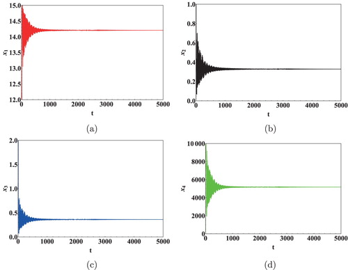
Figure 5. Plots showing the occurrence of periodic solutions of the infected equilibrium $I_1$ when${\tau }_1>{\tau }_1^{\ast }$.

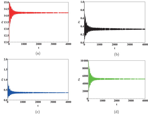
Figure 6. Plots showing the asymptotic stability of the infected equilibrium $I_1$ when ${\tau }_2<{\tau }_2^{\ast }$.

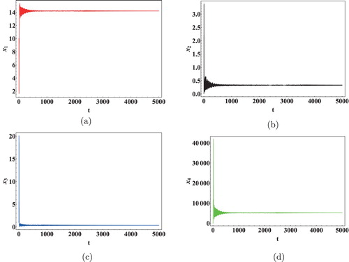
Figure 7. Plots showing the occurrence of periodic solutions of the infected equilibrium $I_1$ when${\tau }_2>{\tau }_2^{\ast }$.

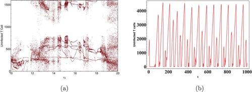
To study the nonlinearity present in the system, Data 3 in Table 2 was used to plot bifurcation diagrams with respect to the time delays. The initial concentration in this case was set to $(800,0.0001,{10}^{-6},0.001)$. The bifurcation diagram and sensitivity analysis plots exhibit the dynamical properties like periodicity, multi-periodicity and chaotic behaviour of the model. The chaotic window in the bifurcation diagram has been determined by checking sensitive dependence on initial conditions of the model Figure 8. Figure 9 shows the bifurcation diagram when ${\tau }_1$ is varied. Initially the solutions are observed to be stable for ${\tau }_1\in (0,1.09)$ days. However, for ${\tau }_1>1.091$ days bifurcation in the system is observed. Similarly for ${\tau }_2\in (0,9.31)$ days, system (1(1) $\begin{array}{r}\begin{array}{rl}{x}_1^{\prime }\left(t\right)& =s-\mathrm{d}{x}_1\left(t\right)-b(1-{ϵ}_r)x_1\left(t\right)x_3\left(t\right)\\ & -\frac{k{x}_1\left(t\right)x_3\left(t\right)}{x_1\left(t\right)+B},\\ x_2^{\prime }\left(t\right)& =b(1-{ϵ}_r)x_1(t-{\tau }_1)x_3(t-{\tau }_1)\\ & -\delta x_2\left(t\right)-d_1{x}_4\left(t\right)x_2\left(t\right),\\ x_3^{\prime }\left(t\right)& =N\delta (1-{ϵ}_p)x_2\left(t\right)-c{x}_3\left(t\right)\\ & -\eta b{x}_3\left(t\right)x_1\left(t\right),\\ x_4^{\prime }\left(t\right)& =p{x}_2(t-{\tau }_2)x_4(t-{\tau }_2)-d_2{x}_4\left(t\right).\end{array}\end{array}$(1) ) was found to be stable and for ${\tau }_2>9.31$ days Hopf bifurcation was observed. In case of ${\tau }_2$, multi-periodicity was also evident as seen from Figure 10. These bifurcation diagrams therefore predict that in long run, the count of T cell and viral load in an HIV infected person under the HAART can sometime lead to no results at all because of abruptly changing count of these cells and virus. Instabilities are thus evident in these kinds of scenario because of nonlinearity present in these systems.

Figure 8. Sensitive dependence of solutions on initial conditions.

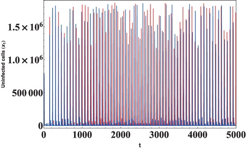
Figure 9. Bifurcation diagram w.r.t. ${\tau }_1$ and corresponding time series plot.

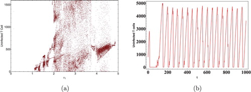
Figure 10. Bifurcation diagram w.r.t. ${\tau }_2$ and corresponding time series plot.

7. Conclusion and discussion

In this article, a delayed model of HIV-1 infection has been studied which includes the apoptosis of cells and loss of virus in the course of infection. This article is an extension of the work discussed by Sahani et al. [36] where only the local stability of the infection-free equilibrium $I_0$ was discussed along with a short discussion of the case when the immunological delay is zero. Here we have extended the work by including a detailed study of the local behaviour of the infected steady $I_1$ and the Hopf bifurcation at the infected steady state. We have also analysed the case when both the delays are non-zero in case of the infected steady state $I_1$. The global stability analysis of the steady states has also been done in this paper.

The effect of apoptosis and virus waning term has been discussed, and from numerical simulation it is clear that an increase in the apoptotic rate of the cells produces more viral cells, thus increasing the viral load. The importance of combination therapy over single drug therapy has also been highlighted in the paper. The graphs for CD4${}^{+}$ T cells plotted show that combination therapy is better in increasing the CD4${}^{+}$ T-cell count. It is also evident from numerical simulations that RTIs are more effective in the combination therapy as compared to PIs.

Bifurcation analysis has been performed on the infected steady state, and the critical value of both the delays has also been calculated. Taking the immunological delay ${\tau }_2$ as zero the critical value of ${\tau }_1$ has been calculated as 11.5 days. Next keeping the value of ${\tau }_1$ in its stability interval the critical value of ${\tau }_2$ was calculated as 0.002 days. By numerical simulation, it has been observed that a slight variation in the value of ${\tau }_2$ generates rich dynamics in the system. Thus, it can be concluded that the intracellular delay doesn't single-handedly affect the system, but when coupled with the intracellular delay generates very rich dynamics. Presence of chaotic solutions for some set of parameters indicates that sometimes the combination drug therapy is not at all effective in containing the virus growth in the body and thus a person infected with HIV will go to the last stage of the disease so called AIDS.

Acknowledgments

The authors are grateful to the esteemed reviewers for their constructive comments and suggestions. They have helped in making the manuscript better in every aspect.

Disclosure statement

No potential conflict of interest was reported by the author.

ORCID

Saroj Kumar Sahani http://orcid.org/0000-0002-8707-033X

Yashi http://orcid.org/0000-0002-1181-9412

Additional information

Funding

This research is fully supported by University Grant Commission (UGC) of India, fellowship scheme 23/06/2013(i)EU-V.

References

- A. Alshorman, X. Wang, M. Joseph Meyer, and L. Rong, Analysis of HIV models with two time delays, J. Biol. Dyn. (2016), pp. 1–25.
- J.J. Bailey, J.E. Fletcher, E.T. Chuck, and R.I. Shrager, A kinetic model of CD4+ lymphocytes with the human immunodeficiency virus, BioSystems 26 (1992), pp. 177–183. doi: 10.1016/0303-2647(92)90077-C
- D. Burg, L. Rong, A.U. Neumann, and H. Dahari, Mathematical modeling of viral kinetics under immune control during primary HIV-1 infection, J. Theor. Biol. 259 (2009), pp. 751–759. doi: 10.1016/j.jtbi.2009.04.010
- M. Ciupe, B. Bivort, D. Bortz, and P. Nelson, Estimating kinetic parameters from HIV primary infection data through the eyes of three different mathematical models, Math. Biosci. 200 (2006), pp. 1–27. doi: 10.1016/j.mbs.2005.12.006
- J.M. Coffin, HIV population dynamics in vivo: Implications for genetic variation, pathogenesis, and therapy, Science 267 (1995), pp. 483–489. doi: 10.1126/science.7824947
- N.W. Cummins and A.D. Badley, Mechanisms of HIV-associated lymphocyte apoptosis: 2010, Cell Death Dis. 1 (2010), p. e99. doi: 10.1038/cddis.2010.77
- E.S. Daar, T. Moudgil, R.D. Meyer, and D.D. Ho, Transient high levels of viremia in patients with primary human immunodeficiency virus type 1 infection, New Engl. J. Med. 324 (1991), pp. 961–964. doi: 10.1056/NEJM199104043241405
- R. Fan, Y. Dong, G. Huang, and Y. Takeuchi, Apoptosis in virus infection dynamics models, J. Biol. Dyn. 8 (2014), pp. 20–41. doi: 10.1080/17513758.2014.895433
- H. Garg, J. Mohl, and A. Joshi, HIV-1 induced bystander apoptosis, Viruses 4 (2012), pp. 3020–3043. doi: 10.3390/v4113020
- M.L. Gougeon, V. Colizzi, A. Dalgleish, and L. Montagnier, New concepts in aids pathogenesis, AIDS Res. Hum. Retroviruses 9 (1993), pp. 287–289. doi: 10.1089/aid.1993.9.287
- R.M. Granich, C.F. Gilks, C. Dye, K.M. De Cock, and B.G. Williams, Universal voluntary HIV testing with immediate antiretroviral therapy as a strategy for elimination of HIV transmission: A mathematical model, Lancet 373 (2009), pp. 48–57. doi: 10.1016/S0140-6736(08)61697-9
- S. Guo and W. Ma, Global behavior of delay differential equations model of HIV infection with apoptosis, Discrete Contin. Dyn. Syst. Ser. B 21 (2016), pp. 103–119. doi: 10.3934/dcdsb.2016.21.103
- J. Heffernan, R. Smith, and L. Wahl, Perspectives on the basic reproductive ratio, J. R. Soc. Interface2 (2005), pp. 281–293. doi: 10.1098/rsif.2005.0042
- J.M. Heffernan and L.M. Wahl, Natural variation in HIV infection: Monte Carlo estimates that include CD8 effector cells, J. Theor. Biol. 243 (2006), pp. 191–204. doi: 10.1016/j.jtbi.2006.05.032
- A. Herz, S. Bonhoeffer, R.M. Anderson, R.M. May, and M.A. Nowak, Viral dynamics in vivo: Limitations on estimates of intracellular delay and virus decay, Proc. Natl. Acad. Sci. 93 (1996), pp. 7247–7251. doi: 10.1073/pnas.93.14.7247
- D.D. Ho, A.U. Neumann, A.S. Perelson, W. Chen, J.M. Leonard, and M. Markowitz, Rapid turnover of plasma virions and CD4 lymphocytes in HIV-1 infection, Nature 373 (1995), pp. 123–126. doi: 10.1038/373123a0
- E. Jacotot, L. Ravagnan, M. Loeffler, K.F. Ferri, H.L. Vieira, N. Zamzami, P. Costantini, S.Druillennec, J. Hoebeke, J.P. Briand, T. Irinopoulou, E. Daugas, S.A. Susin, D. Cointe, Z.H. Xie, J.C.Reed, B.P. Roques, and G. Kroemer, The HIV-1 viral protein R induces apoptosis via a direct effect on the mitochondrial permeability transition pore, J. Exp. Med. 191 (2000), pp. 33–46. doi: 10.1084/jem.191.1.33
- X. Jiang, X. Zhou, X. Shi, and X. Song, Analysis of stability and Hopf bifurcation for a delay-differential equation model of HIV infection of CD4+ T-cells, Chaos Solitons Fractals 38 (2008), pp. 447–460. doi: 10.1016/j.chaos.2006.11.026
- D. Kirschner, Using mathematics to understand HIV immune dynamics. AMS Notices 43 (1996), pp. 191–202.
- C.J. Li, D.J. Friedman, C. Wang, V. Metelev, and A.B. Pardee, Induction of apoptosis in uninfected lymphocytes by HIV-1 Tat protein, Science 268 (1995), p. 429. doi: 10.1126/science.7716549
- G. Magombedze, W. Garira, and E. Mwenje, Modeling the TB/HIV-1 co-infection and the effects of its treatment, Math. Popul. Stud. 17 (2010), pp. 12–64. doi: 10.1080/08898480903467241
- G. Magombedze, W. Garira, E. Mwenje, and C.P. Bhunu, Optimal control for HIV-1 multi-drug therapy, Int. J. Comput. Math. 88 (2011), pp. 314–340. doi: 10.1080/00207160903443755
- S.J. Merrill, Modeling the interaction of HIV with cells of the immune system, in Mathematical and Statistical Approaches to AIDS Epidemiology, C. Castillo-Chavez, ed., Springer, Berlin, Heidelberg, 1989, pp. 371–385.
- J.M. Murray, S. Emery, A.D. Kelleher, M. Law, J. Chen, D.J. Hazuda, B.Y.T. Nguyen, H. Teppler, and D.A. Cooper, Antiretroviral therapy with the integrase inhibitor raltegravir alters decay kinetics of HIV, significantly reducing the second phase, Aids 21 (2007), pp. 2315–2321. doi: 10.1097/QAD.0b013e3282f12377
- S.D. Musekwa, T. Shiri, and W. Garira, A two-strain HIV-1 mathematical model to assess the effects of chemotherapy on disease parameters, Math. Biosci. Eng. 2 (2005), pp. 811–32. doi: 10.3934/mbe.2005.2.811
- M.A. Nowak and C.R. Bangham, Population dynamics of immune responses to persistent viruses, Science 272 (1996), pp. 74–79. doi: 10.1126/science.272.5258.74
- M. Nowak and R.M. May, Virus Dynamics: Mathematical Principles of Immunology and Virology, Oxford University Press, 2000.
- R. Ouifki and G. Witten, Stability analysis of a model for HIV infection with RTI and three intracellular delays, BioSystems 95 (2009), pp. 1–6. doi: 10.1016/j.biosystems.2008.05.027
- K.A. Pawelek, S. Liu, F. Pahlevani, and L. Rong, A model of HIV-1 infection with two time delays: Mathematical analysis and comparison with patient data, Math. Biosci. 235 (2012), pp. 98–109. doi: 10.1016/j.mbs.2011.11.002
- A.S. Perelson, D.E. Kirschner, and R. De Boer, Dynamics of HIV infection of CD4+ T cells, Math. Biosci. 114 (1993), pp. 81–125. doi: 10.1016/0025-5564(93)90043-A
- A.S. Perelson, A.U. Neumann, M. Markowitz, J.M. Leonard, and D.D. Ho, HIV-1 dynamics in vivo: Virion clearance rate, infected cell life-span, and viral generation time, Science 271 (1996), pp. 1582–1586. doi: 10.1126/science.271.5255.1582
- M. Pitchaimani, C. Monica, and M. Divya, Stability analysis for HIV infection delay model with protease inhibitor, BioSystems 114 (2013), pp. 118–124. doi: 10.1016/j.biosystems.2013.08.003
- S.M. Raimundo, H.M. Yang, E. Venturino, and E. Massad, Modeling the emergence of HIV-1 drug resistance resulting from antiretroviral therapy: Insights from theoretical and numerical studies, BioSystems 108 (2012), pp. 1–13. doi: 10.1016/j.biosystems.2011.11.009
- L. Rong, Z. Feng, and A.S. Perelson, Mathematical analysis of age-structured HIV-1 dynamics with combination antiretroviral therapy, SIAM J. Appl. Math. 67 (2007), pp. 731–756. doi: 10.1137/060663945
- M.A. Safi, Global dynamics of treatment models with time delay. Comput. Appl. Math. 34 (2014), pp. 1–17.
- S.K. Sahani, et al. Analysis of a delayed HIV infection model, International Workshop on Computational Intelligence (IWCI), IEEE, 2016, pp. 246–251.
- N. Selliah and T. Finkel, Biochemical mechanisms of HIV induced T cell apoptosis, Cell Death Diff.8 (2001), pp. 127–136. doi: 10.1038/sj.cdd.4400822
- H.L. Smith and P. De Leenheer, Virus dynamics: A global analysis, SIAM J. Appl. Math. 63 (2003), pp. 1313–1327. doi: 10.1137/S0036139902406905
- H. Song, W. Jiang, and S. Liu, Virus dynamics model with intracellular delays and immune response, Math. Biosci. Eng. 12 (2015), pp. 185–208.
- P. Srivastava, M. Banerjee, and P. Chandra, Modeling the drug therapy for HIV infection, J. Biol. Syst. 17 (2009), pp. 213–223. doi: 10.1142/S0218339009002764
- J. Tam, Delay effect in a model for virus replication, Math. Med. Biol. 16 (1999), pp. 29–37. doi: 10.1093/imammb/16.1.29
- H.R. Thieme, Mathematics in Population Biology, Princeton University Press, 2003.
- K. Wang, W. Wang, H. Pang, and X. Liu, Complex dynamic behavior in a viral model with delayed immune response, Physica D 226 (2007), pp. 197–208. doi: 10.1016/j.physd.2006.12.001
- T. Wang, Z. Hu, and F. Liao, Stability and Hopf bifurcation for a virus infection model with delayed humoral immunity response, J. Math. Anal. Appl. 411 (2014), pp. 63–74. doi: 10.1016/j.jmaa.2013.09.035
- Y. Wang, F. Brauer, J. Wu, and J.M. Heffernan, A delay-dependent model with HIV drug resistance during therapy, J. Math. Anal. Appl. 414 (2014), pp. 514–531. doi: 10.1016/j.jmaa.2013.12.064
- Y. Wang, Y. Zhou, F. Brauer, and J.M. Heffernan, Viral dynamics model with CTL immune response incorporating antiretroviral therapy, J. Math. Biol. 67 (2013), pp. 901–934. doi: 10.1007/s00285-012-0580-3
- Z. Wang and R. Xu, Stability and Hopf bifurcation in a viral infection model with nonlinear incidence rate and delayed immune response, Commun. Nonlinear Sci. Numer. Simul. 17 (2012), pp. 964–978. doi: 10.1016/j.cnsns.2011.06.024
- H. Zhu, Y. Luo, and M. Chen, Stability and Hopf bifurcation of a HIV infection model with CTL-response delay, Comput. Math. Appl. 62 (2011), pp. 3091–3102. doi: 10.1016/j.camwa.2011.08.022
- H. Zhu and X. Zou, Dynamics of a HIV-1 infection model with cell-mediated immune response and intracellular delay, Discrete Contin. Dyn. Syst. Ser. B 12 (2009), pp. 511–524. doi: 10.3934/dcdsb.2009.12.511