
 ?Mathematical formulae have been encoded as MathML and are displayed in this HTML version using MathJax in order to improve their display. Uncheck the box to turn MathJax off. This feature requires Javascript. Click on a formula to zoom.
ABSTRACT
In this study, we first formulate a baseline discrete-time mathematical model for malaria transmission where the survival function of mosquitoes is of Beverton–Holt type. We then introduce sterile mosquitoes to the baseline model to explore the transmission dynamics with sterile mosquitoes. We derive formulas for the reproductive number of infection and determine the existence and uniqueness of endemic fixed points as well, for the models with or without sterile mosquitoes. We then study the impact of the releases of sterile mosquitoes on the disease transmissions by investigating the effects of varying the release rates of the sterile mosquitoes. We use a numerical example to illustrate our results for all cases and finally give brief discussions of our findings.
1. Introduction
Mosquito-borne diseases, such as malaria, are a big concern for the public health worldwide. Malaria is a leading cause of death in many developing countries. There are 3.2 billion people, half of the world's population, living in areas at risk of malaria transmission in 106 countries and territories. In 2016, estimated 216 million cases of malaria occurred worldwide and 445,000 people died, mostly children in the African Region. About 1700 cases of malaria are diagnosed in the United States each year [Citation13, Citation23, Citation30].
Malaria is transmitted indirectly not from a human to a human but through vectors as blood-feeding mosquitoes. The effective way to prevent the transmission of such diseases is to control mosquitoes and among the biological methods in control of mosquitoes is the sterile insect technique (SIT) [Citation7], in which the natural reproductive process of the target population is disrupted. By chemical or physical methods, male mosquitoes are genetically modified to be sterile despite being sexually active. These sterile male mosquitoes are then released into the environment to mate with the wild female mosquitoes. A wild female mosquito that mates with a sterile male mosquito will either not reproduce or produce eggs that do not hatch. Repeated releases of genetically modified mosquitoes or the releases of a significantly large number of sterile mosquitoes may eventually wipe out a wild mosquito population, although it is, in practice, often more useful to consider controlling the population rather than eradicating it [Citation5, Citation8, Citation29].
Mathematical models have played an important role in providing insights into the transmission dynamics of diseases and in influencing the decision making for preventing the diseases. There are many models in the literature for the study of vector-borne diseases and models incorporating sterile mosquitoes, are also formulated for the disease transmission dynamics [Citation1, Citation9, Citation17, Citation18, Citation20, Citation28]. However, most of the models are of continuous time, based on differential equations, to take advantage of the rich theoretical foundation of the well-developed dynamical systems theory and bifurcation theory. As time steps are sufficiently small or population sizes are sufficiently large, these models are valid. The results from those continuous-time models have shown their significance in helping understand the transmission dynamics and make useful strategies for control and prevention of the disease.
On the other hand, the timescales for the dynamics of the human and mosquito populations are significantly different. Then, discrete-time models, based on difference equations, become equally important and even more appropriate [Citation3, Citation10, Citation11, Citation14]. Moreover, discrete-time models also have many strengths in the theory of population dynamics and mathematical epidemiology [Citation2, Citation10, Citation11, Citation27, Citation31].
In this paper, we first formulate a discrete-time susceptible-exposed-infective-recovered (SEIR) compartmental model for humans and a susceptible-exposed-infective (SEI) compartmental model for mosquitoes, based on the model in [Citation21], as our baseline model in Section 2. We derive a formula for the reproductive number of infection and study the existence of endemic fixed points. We then incorporate the sterile mosquitoes into the baseline model such that the susceptible mosquitoes consist of wild and sterile mosquitoes in Section 3. We consider the case where the release rate of sterile mosquitoes is constant and derive a formula for the reproductive number. We investigate the impact of the releases of sterile mosquitoes on the malaria transmission based on the reproductive number and the endemic fixed points, and give a numerical example to verify our theoretical results in Section 4. Brief discussions of our findings are provided in Section 5.
2. Baseline model for malaria transmission
To study the impact of interactive wild and sterile mosquitoes on the malaria transmission, based on the discrete-time malaria model in [Citation21], we formulate a new discrete-time model as our baseline model in this section, where the survivability of mosquitoes assumes the Beverton–Holt type of nonlinearity instead of the Ricker type in [Citation21].
Since the mosquitoes lifespan is shorter than their infective period, we assume that mosquitoes are unable to recover after infection. Then we divide the mosquito population into groups of susceptible, exposed or incubating, and infective individuals, and denote their numbers, at generation n, by ,
and
, respectively [Citation6, Citation21].
For the human population, we divide it into groups of susceptible, exposed or incubating, infective and recovered individuals. We let be the number of susceptible humans,
the number of exposed or incubating humans who are infected but not infectious yet,
the number of infective humans who are infected and also infectious,
the number of humans who are recovered from infection but partly lose their immunity [Citation19, Citation24–26], and
, the total number of humans at time n.
Then, the model equations for humans and mosquitoes described in Figure are given by
(2.1)
(2.1) where the parameters are given in Table . We assume that the infection has no effects on the birth and that the intraspecific competition only affects the survivability of the susceptible newborns. We further assume that the survivability of the susceptible newborns,
, has the Beverton–Holt-II type of nonlinearity as
(2.2)
(2.2)
Figure 1. Schematic diagram for the malaria transmission. The mosquito population is divided into three groups, ,
and
and the human population is divided into four groups,
,
,
and
. The mosquito infection rate
is given in (Equation2.3
(2.3)
(2.3) ), and the human infection rate
is given in (Equation2.5
(2.5)
(2.5) ).
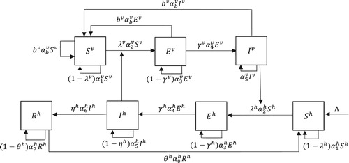
Table 1. The parameters for the malaria transmission model.
To determine the infection rates and
, we let r be the average number of bites that a single mosquito makes on all human hosts. Then the total number of bites made by susceptible mosquitoes is
, among which, a proportion of
goes to the infected hosts, causing
new infections for mosquitoes, where
is the transmission probability per bite to a susceptible mosquito. Thus the infection rate for mosquitoes is given by
(2.3)
(2.3) where we assume
.
Similarly, let be the average number of bites a human host receives from all mosquitoes. Then the total number of bites received by susceptible human hosts is
, among which, a proportion of
is from infected mosquitoes, causing
new infections for hosts, where
is the transmission probability per bite to a susceptible human. Here, however, we need to note that the number of infected mosquitoes can be sufficiently larger than the total number of humans, that is,
. Then, it may lead to the human infection rate greater than 1 even when
, and thus
from (Equation2.1
(2.1)
(2.1) ), if we directly define
in the same way as for
. Thus we consider the following factor for the infection rate for humans:
(2.4)
(2.4) Moreover, the total number of bites that all mosquitoes make is the same as the total number of bites all human hosts receive. We then need the following balance constraint:
and this balance constraint and (Equation2.4
(2.4)
(2.4) ) immediately lead to
Since the number of infected mosquitoes can be sufficiently larger than the total number of humans, which may lead to the factor
much greater than 1, we assume that the infection rate for humans is given by
(2.5)
(2.5) where G is a positive function of L, satisfying the following conditions [Citation10]:
(2.6)
(2.6)
2.1. The reproductive number
We derive a formula for the reproductive number by investigating the local stability of the infection-free fixed point. The Jacobian matrix of system (Equation2.1(2.1)
(2.1) ) at the infection-free fixed point
with
(2.7)
(2.7) has the form
(2.8)
(2.8) where F is the fertility matrix given by
T is the transition matrix given by
and matrix C has the form
where
since
Then, the next generation matrix of system (Equation2.1
(2.1)
(2.1) ) [Citation4, Citation12, Citation15, Citation16] is given by
where
The characteristic polynomial of Q is
which leads to the eigenvalues as
and
. According to [Citation16], the infection-free fixed point is locally asymptotically stable if and only if the eigenvalues
. Thus we define the net reproductive number of infection as
.
Hence,
(2.9)
(2.9) with
and
given in (Equation2.7
(2.7)
(2.7) ).
We have the following results.
Theorem 2.1
Define the reproductive number of infection, in (Equation2.9
(2.9)
(2.9) ) for system (Equation2.1
(2.1)
(2.1) ). Then, the infection-free fixed point is locally asymptotically stable if
and is unstable if
.
2.2. The endemic fixed point
We next explore the existence of endemic fixed points of system (Equation2.1(2.1)
(2.1) ).
The components of an endemic fixed point need to satisfy the following equations:
(2.10a)
(2.10a)
(2.10b)
(2.10b)
(2.10c)
(2.10c)
(2.10d)
(2.10d)
(2.10e)
(2.10e)
(2.10f)
(2.10f)
(2.10g)
(2.10g)
Solving (Equation2.10a(2.10a)
(2.10a) )–(Equation2.10d
(2.10d)
(2.10d) ), we have
(2.11)
(2.11) where
Then we have
(2.12)
(2.12) where
.
Solving (Equation2.10e(2.10e)
(2.10e) )–(Equation2.10g
(2.10g)
(2.10g) ), we have
(2.13)
(2.13) where
(2.14)
(2.14) Substituting (Equation2.11
(2.11)
(2.11) )–(Equation2.13
(2.13)
(2.13) ) into (Equation2.3
(2.3)
(2.3) ) and (Equation2.5
(2.5)
(2.5) ), respectively, we obtain
(2.15)
(2.15) and
Hence, there exists an endemic fixed point if and only if there is a positive solution to equation
, or equivalently,
for
.
Notice that and hence
by (Equation2.6
(2.6)
(2.6) ). Then
and
since
and
. Moreover, it follows from
and
that
Thus if
, there exists a positive solution to
, that is, to
. In other words, there exists an endemic fixed point if
.
Theorem 2.2
For system (Equation2.1(2.1)
(2.1) ), if the reproductive number
there exits an endemic fixed point.
3. The interactive transmission model with sterile mosquitoes
Now suppose that sterile mosquitoes are released into a wild mosquito population and we let be the number of the sterile mosquitoes released at time n. Since sterile mosquitoes do not reproduce, there is no maturation process from larvae to adults for sterile mosquitoes. Hence, the number of sterile mosquitoes at n is just the number of released sterile mosquitoes, and the size of total mosquitoes is
. We assume sterile mosquitoes are constantly released such that
is a positive constant. After the sterile mosquitoes are released, the mating interaction between the wild and sterile mosquitoes takes place. The number of susceptible offspring produced per mating is
Then the model for the interactive mosquitoes and the human population can be described as
(3.1)
(3.1) where the human part remains the same as described in system (Equation2.1
(2.1)
(2.1) ).
Assume that all of the survival probabilities of mosquitoes ,
, in system (Equation3.1
(3.1)
(3.1) ) are the same, denoted by
. Then the interactive dynamics between the total wild mosquitoes and the constant sterile mosquitoes are governed by the following equation:
(3.2)
(3.2) It follows from [Citation22] that the results for (Equation3.2
(3.2)
(3.2) ) can be stated as follows.
Lemma 3.1
Theorem 4.1 [Citation22]
For given system (Equation3.2
(3.2)
(3.2) ) has no, one or two positive fixed points if
or
respectively, where the release threshold
is given by
(3.3)
(3.3) If
there exists no positive fixed point and
is the only fixed point, which is globally asymptotically stable. Thus the wild mosquito population goes extinct regardless of the initial population size. If
there exists a unique positive fixed point which is unstable and thus the trivial fixed point
is also globally asymptotically stable. If
there exist two positive fixed points
(3.4)
(3.4) where
is unstable and
is locally asymptotically stable with a basin of attraction
while the trivial fixed point
is locally asymptotically stable with a basin of attraction
.
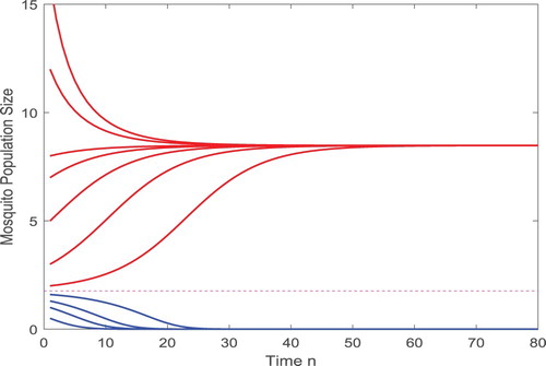
Notice that if , for system (Equation3.2
(3.2)
(3.2) ), there exists no positive fixed point and the trivial fixed point
is the only fixed point, which is globally asymptotically stable. Correspondingly, for system (Equation3.1
(3.1)
(3.1) ), all wild mosquitoes eventually go extinct so that there will be no malaria transmission. Thus we only consider the case of
, and we assume the initial size of the wild mosquitoes is greater than
, as shown in Figure .
Figure 2. Solutions approach or
depending on their initial values.
3.1. The reproductive number and disease spread
We derive a formula for the reproductive number of infection after the sterile mosquitoes are released into the wild mosquito population with and the initial size in
as follows.
Consider the following infection-free fixed point of system (Equation3.1(3.1)
(3.1) ):
It follows from (Equation2.7
(2.7)
(2.7) ) that
and from (Equation3.1
(3.1)
(3.1) ) that
(3.5)
(3.5) We then define function
by
(3.6)
(3.6) Clearly, there exists no, one or two positive roots of (Equation3.6
(3.6)
(3.6) ) if
,
or
, respectively, where
is given in (Equation3.3
(3.3)
(3.3) ). Therefore, in the case of
, there exist two infection-free fixed points.
The Jacobian matrix evaluated at an infection-free fixed point has the following form:
where
is the fertility matrix
,
is the transition matrix
, with F and T given in (Equation2.8
(2.8)
(2.8) ), and
with
It follows from (Equation3.6
(3.6)
(3.6) ) that
which implies that, for the two positive roots
,
that is,
Thus we have
for
, and hence
is unstable.
On the other hand, it follows from for
that all eigenvalues of matrix C are inside the unit circle, and thus the local stability of this infection-free fixed point is determined by matrix
. It follows then from Section 2.1 that we can define the reproductive number of infection for system (Equation3.1
(3.1)
(3.1) ) as
(3.7)
(3.7) where
equals
given in (Equation3.4
(3.4)
(3.4) ).
By using b as a variable, is a function of b and so is
. When b=0, it is clear that
and
. Then
and, for
,
. Thus
.
It follows from (Equation3.6(3.6)
(3.6) ) that
and we have
(3.8)
(3.8) Since
,
is monotone decreasing with respect to b. Notice that function
is monotone increasing with respect to
. That is to say, the composed function
is monotone decreasing with respect to b. Hence, there is a unique threshold
such that
and
In fact, the threshold
can be explicitly solved as follows.
Since , we have
It follows from (Equation3.5
(3.5)
(3.5) ) that
(3.9)
(3.9) Thus, the infection-free fixed point of system (Equation3.1
(3.1)
(3.1) ) is locally asymptotically stable if
and unstable if
. We also notice that if
, the infection-free fixed point with the unique positive component
is unstable and if
, there exists no such positive component
. Thus all wild mosquitoes will be wiped out if
and hence
. We summarize the results as follows.
Theorem 3.1
Assume sterile mosquitoes are released into the wild mosquito population constantly with the number of releases b>0. Define the two threshold values of releases and
in (Equation3.3
(3.3)
(3.3) ) and (Equation3.9
(3.9)
(3.9) ), respectively. Then we have the following results.
If
there exists no positive fixed point for the interactive mosquitoes system (Equation3.2
If
If
If
3.2. Endemic fixed point
Similarly as in Section 2.2, we determine the existence of endemic fixed points for system (Equation3.1(3.1)
(3.1) ) as follows.
The components of an endemic fixed point for the human part are the same as those in Section 2.2 for the baseline model. The components for the wild mosquitoes at an endemic fixed point satisfy the following system:
(3.10a)
(3.10a)
(3.10b)
(3.10b)
(3.10c)
(3.10c) which leads to
with
for
. Then
given in (Equation3.4
(3.4)
(3.4) ).
Solving (Equation3.10a(3.10a)
(3.10a) )–(Equation3.10c
(3.10c)
(3.10c) ), we have
(3.11)
(3.11) where
and
are defined in (Equation2.14
(2.14)
(2.14) ). Then we obtain
(3.12)
(3.12) Substituting (Equation3.11
(3.11)
(3.11) ) and (Equation2.15
(2.15)
(2.15) ) into
in (Equation2.5
(2.5)
(2.5) ) yields
It follows from (Equation3.12
(3.12)
(3.12) ) that
Then
(3.13)
(3.13) where
and
. Hence, there exists an endemic fixed point if and only if there is a positive solution to equation
, or equivalently,
(3.14)
(3.14) for
.
Notice that and hence
by (Equation2.6
(2.6)
(2.6) ). Then
and
since
and
. Moreover, it follows from
that
Thus if
, there exists a positive solution
to
, that is, to
. Then there exists an endemic fixed point if
.
Next, we prove the uniqueness of this endemic fixed point.
We rewrite the equation as
for convenience and take the first derivative with respect to variable x. Then we have
where
. It follows from (Equation3.13
(3.13)
(3.13) ) that
where
and we write
(3.15)
(3.15) If k<0, there exists a unique positive solution
satisfying
. Then
if
and
which leads to
if
. Thus
is monotone decreasing if
.
We then prove that is monotone decreasing for
, which is equivalent to
for
.
It follows from (Equation3.13(3.13)
(3.13) ) that
where
(3.16)
(3.16) Since
from (Equation3.15
(3.15)
(3.15) ) with k<0, the constant part of function
becomes
Hence there exists at most one positive solution
satisfying
from Descartes' rule of sign. Thus
if
and
if
.
In order to compare with
, we assume
. Then, for any
,
is increasing and
but
, which is a contradiction. Thus,
, and then
for
. It follows from
(3.17)
(3.17) where
, that
for
. Therefore, function
is concave down for
and then decreasing for
with
, which implies that the endemic fixed point is unique.
If k>0, then and thus
for all x. If the constant part of
from (Equation3.16
(3.16)
(3.16) ) is negative,
for all
and thus
, which implies that
from (Equation3.17
(3.17)
(3.17) ). Since function
is concave down for all
, the endemic fixed point is unique.
If the constant part of from (Equation3.16
(3.16)
(3.16) ) is positive, there exists a unique solution
such that
. Then
if
and
if
. Hence
is monotone increasing if
and monotone decreasing if
with
, where there exists a unique solution
such that
. Therefore, function
is monotone increasing for
and monotone decreasing for
. Thus the endemic fixed point is unique.
In summary, we have shown that when , the infection-free fixed point is unstable and there exists a unique endemic fixed point.
In the following, we prove that if , there exists no endemic fixed point.
If k<0, it follows from the analysis above that is concave down if
and monotone decreasing if
. Thus there exists no intersection with x-axis since
.
If k>0, it follows from (Equation3.16(3.16)
(3.16) ) that
is concave down with
if the constant part of
is negative, and hence there exists no endemic fixed point. On the other hand, if the constant part of
is positive,
is monotone increasing if
and monotone decreasing if
with
. Thus
and
since
from (Equation3.17
(3.17)
(3.17) ). Then
, which implies that
for all
. Hence
is monotone decreasing for all
and there exists no endemic fixed point.
4. Impact of releases of sterile mosquitoes
To study the impact of the releases of sterile mosquitoes on the malaria transmission dynamics, first, it is clear that if , there is no infection. We then consider the interval
, where
is given in (Equation3.9
(3.9)
(3.9) ). For each
, the corresponding reproductive number
and there exists a unique endemic fixed point associated with
to equation
.
With this , we have
Then it follows from (Equation3.13
(3.13)
(3.13) ) that
since both
and
can be regarded as functions of variable b. Thus
(4.1)
(4.1) and by taking the derivative of equation
with respect to b on both sides,
Equivalently,
(4.2)
(4.2) where
and
. Hence
, which implies that
is monotone decreasing with respect to b.
Moreover, it follows from (Equation2.11(2.11)
(2.11) ) that
and then
Thus component
of the unique endemic fixed point is monotone decreasing with respect to b. In other words, we can reduce the population of the infected humans by increasing the amount of sterile mosquitoes.
Furthermore, it follows from (Equation3.11(3.11)
(3.11) ) and (Equation3.12
(3.12)
(3.12) ) that
Taking the derivative with respect to b, we obtain
In addition, it follows from (Equation2.15
(2.15)
(2.15) ) that
and
from (Equation3.8
(3.8)
(3.8) ). Consequently,
, which implies that component
of the unique endemic fixed point is also monotone decreasing with respect to b. As a result of increasing the releases of the sterile mosquitoes, we can possibly wipe out all of the wild mosquitoes eventually.
Therefore, for , even though
such that the disease spreads and goes to a positive steady state for
, we can still reduce the components of the infected humans and mosquitoes by increasing the releases of the sterile mosquitoes to make the transmission under control.
We provide an example below to demonstrate our findings.
Example 4.1
We use the following parameters for the transmission model:
(4.3)
(4.3) and
.
Before the sterile mosquitoes are released, the reproductive number of infection for system (Equation2.1(2.1)
(2.1) ) is
and hence the disease spreads. After the releases of sterile mosquitoes, we have the existence threshold value
such that if b=45>42.0743, there exists no positive fixed point and thus the infection eventually dies out, as shown in Figure . If b<42.0743, there exist two positive fixed points with components
where
is unstable and
is locally asymptotically stable with initial value larger than
.
is a decreasing function with respect to release value b.
Figure 3. With the parameters given in (Equation4.3(4.3)
(4.3) ), the threshold value is
. If
, the trivial fixed point is globally asymptotically stable, which leads to the infection eventually extinct as shown above.
However, the threshold value for the disease spread is such that the reproductive number
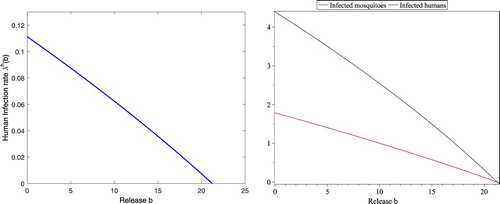
if b=30>21.2330 and thus the disease dies out eventually, which is shown in Figure (right). If b<21.2330, the reproductive number
, which makes the infection-free fixed point unstable and thus the disease spreads. Moreover,
is monotone decreasing with respect to b, as shown in Figure (left).
Figure 4. With the same parameters in (Equation4.3(4.3)
(4.3) ), the threshold values are
and
, respectively. By using b as a variable, the horizontal axis is for b and the vertical axis is for
(left). The reproductive number
at b=0. For b=30, the infection-free fixed point is stable since
. Then the infected humans and infected mosquitoes eventually go extinct (right).
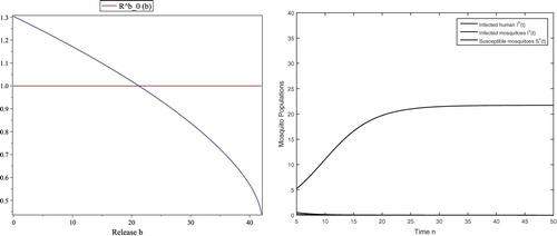
For b<21.2330, , the corresponding
determined in (Equation3.14
(3.14)
(3.14) ) is a positive and decreasing function as shown in Figure (left). Corresponding to
, there exists a unique endemic fixed point whose components
and
are monotone decreasing with respect to b as shown in Figure (right), which indicates that increasing the releases of sterile mosquitoes reduces the disease spread.
Figure 5. With still the same parameters in (Equation4.3(4.3)
(4.3) ), the threshold values are
and
, respectively. The curve on the left figure is for
at the endemic fixed point for each b. The upper curve and lower curve on the right figure are for
and
at the endemic fixed point for each b, respectively. Clearly,
,
and
are all negative if
, which implies that no endemic fixed point exists although positive
exists for
.
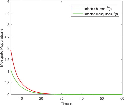
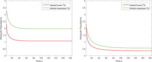
To show the dynamical impact of the releases of the sterile mosquitoes, we also present the solutions of the disease transmission system in Figure . When no sterile mosquitoes are released, the reproductive number and the disease spreads as shown in Figure (left). For
, the reproductive number
such that the infection still exists but the number of infected humans and infected mosquitoes are reduced significantly as shown in Figure (right).
Figure 6. (Left) With again the parameters given in (Equation4.3(4.3)
(4.3) ), the reproductive number is
and hence the disease spreads in the absence of sterile mosquitoes. (Right) After the sterile mosquitoes are released, even the released amount is less than the threshold with
, the infected components
and
are reduced so that we can have the infection under control.
5. Concluding remarks
To have a better understanding of the impact of releasing sterile mosquitoes on malaria transmission, we first formulated a simple compartmental SEIR model for the malaria transmission, the survivability of the susceptible newborns has the Beverton–Holt-II type of nonlinearity, in (Equation2.1(2.1)
(2.1) ) as our baseline model in Section 2. We derived a formula for the reproductive number of infection
in (Equation2.9
(2.9)
(2.9) ) and showed that the infection-free fixed point of the baseline model is asymptotically stable if
and unstable if
. We also showed that if
, there exists an endemic fixed point for the baseline model.
We then introduced sterile mosquitoes into our baseline model and formulated the interactive model in Section 3. The human components are the same as those in (Equation2.1(2.1)
(2.1) ) but the mosquito components are given in (Equation3.1
(3.1)
(3.1) ). We only consider the case of constant releases of sterile mosquitoes. We derived a formula for the reproductive number
, presented in (Equation3.7
(3.7)
(3.7) ), and showed
for any release amount b. We proved that the infection-free fixed point is asymptotically stable if
and is unstable if
. Using the rate of releases b as a variable, we determined threshold value
for the existence of a unique endemic fixed point for the interactive wild and sterile mosquitoes and threshold value
that determines whether
or
, that is, whether the disease dies out or spreads.
We studied the impact of the releases of sterile mosquitoes on the transmission dynamics in Section 4 by investigating the variation of the reproductive number, , and the infected components,
and
, induced by
, as b varies, respectively. Based on the threshold values
and
, we provided Example 4.1 to confirm and demonstrate our findings. If the rate of releases b is greater than threshold
, the trivial fixed point for the interactive wild and sterile mosquitoes is locally asymptotically stable. All wild mosquitoes are wiped out and thus there is no infection. On the other hand, if
, while the wild mosquitoes cannot be wiped out and the two types of mosquitoes coexist, the disease can still go extinct when there are sufficient sterile mosquitoes with
, which leads to
. In the case even if we are unable to release enough sterile mosquitoes with
, which leads to
and thus the disease spreads when the initial wild mosquitoes is larger than
given in (Equation3.4
(3.4)
(3.4) ), the infected components
and
are monotone decreasing with respect to b; that is, the infection can be reduced. All of the results are demonstrated by numerical simulations in Example 4.1.
In conclusion, based on the discrete-time interactive malaria model we formulated and the analysis we accomplished in this study, we showed that the releases of sterile mosquitoes have significant impacts on controlling the transmission of malaria. It will be useful and helpful in considering effective strategies for control and prevention of mosquito-borne diseases as well.
Disclosure statement
No potential conflict of interest was reported by the authors.
References
- S. Ai, J. Lu, and J. Li, Mosquito-stage-structured malaria models and their global dynamics, SIAM J. Appl. Math. 72 (2012), pp. 1223–1237. doi: 10.1137/110860318
- L.J.S. Allen, Some discrete-time SI, SIR, and SIS epidemic models, Math. Biosci. 124 (1994), pp. 83–105. doi: 10.1016/0025-5564(94)90025-6
- L.J.S. Allen and A.M. Burgin, Comparison of deterministic and stochastic SIS and SIR models in discrete-time, Math. Biosci. 163 (2000), pp. 1–33. doi: 10.1016/S0025-5564(99)00047-4
- L.J.S. Allen and P. van den Driessche, The basic reproduction number in some discrete-time epidemic models, J. Difference Equ. Appl. 14 (2008), pp. 1127–1147. doi: 10.1080/10236190802332308
- L. Alphey, M. Benedict, R. Bellini, G.G. Clark, D.A. Dame, M.W. Service, and S.L. Dobson, Sterile-insect methods for control of mosquito-borne diseases: an analysis, Vector Borne Zoonotic Dis.10 (2010), pp. 295–311. doi: 10.1089/vbz.2009.0014
- R.M. Anderson and R.M. May, Infectious Disease of Humans, Dynamics and Control, Oxford University Press, New York, 1991.
- H.J. Barclay and M. Mackuer, The sterile insect release method for pest control: a density dependent model, Environ. Entomol. 9 (1980), pp. 810–817. doi: 10.1093/ee/9.6.810
- A.C. Bartlett and R.T. Staten, Sterile Insect Release Method and Other Genetic Control Strategies, Radcliffe's IPM World Textbook, St. Paul, 1996.
- L. Cai, S. Ai, and J. Li, Dynamics of mosquitoes populations with different strategies for releasing sterile mosquitoes, SIAM J. Appl. Math. 74 (2014), pp. 1786–1809. doi: 10.1137/13094102X
- C. Castillo-Chavez and A. Yakubu, Discrete-time S-I-S models with complex dynamics, Nonlinear Anal. 47 (2001), pp. 4753–4762. doi: 10.1016/S0362-546X(01)00587-9
- C. Castillo-Chavez and A. Yakubu, Discrete-time S-I-S models with simple and complex population dynamics, in Mathematical Approaches for Emerging and Reemerging Infectious Diseases: An Introduction, IMA, C. Castillo-Chavez, S. Blower, P. van den Driessche, D. Kirschner, and A. Yakubu, eds., Vol. 125, Springer-Verlag, New York, 2002, pp. 153–163.
- H. Caswell, Matrix Population Models, 2nd ed., Sinauer Associatis, Inc., Sunderland, MA, 2001.
- CDC, Malaria. 2018. Available at https://www.cdc.gov/parasites/malaria/.
- N. Chitnis, T. Smith, and R. Steketee, A mathematical model for the dynamics of malaria in mosquitoes feeding on heterogeneous host population, J. Biol. Dyn. 3 (2008), pp. 259–285. doi: 10.1080/17513750701769857
- J.M. Cushing, An Introduction to Structured Population Dynamics, SIAM, Philadelphia, PA, 1998.
- J.M. Cushing and Z. Yicang, The net reproductive value and stability in matrix population models. Nat. Res. Model. 8 (1994), pp. 297–333. doi: 10.1111/j.1939-7445.1994.tb00188.x
- Y. Dumont and J.M. Tchuenche, Mathematical studies on the sterile insect technique for the Chikungunya disease and Aedes albopictus, J. Math. Biol. 65 (2012), pp. 809–854. doi: 10.1007/s00285-011-0477-6
- L. Esteva and H.M. Yang, Mathematical model to assess the control of Aedes aegypti mosquitoes by the sterile insect technique, Math. Biosci. 198 (2005), pp. 132–147. doi: 10.1016/j.mbs.2005.06.004
- J. Li, Malaria models with partial immunity in humans, Math. Biol. Eng. 5 (2008), pp. 789–801. doi: 10.3934/mbe.2008.5.789
- J. Li, Malaria model with stage-structured mosquitoes, Math. Biol. Eng. 8 (2011), pp. 753–768. doi: 10.3934/mbe.2011.8.753
- J. Li, Simple discrete-time malarial models, J. Diff. Eq. Appl. 19 (2013), pp. 649–666. doi: 10.1080/10236198.2012.672566
- Y. Li and J. Li, Discrete-time models for releases of sterile mosquitoes with Beverton–Holt-type of survivability, Ricerche mat. 67 (2018), pp. 141–162. doi: 10.1007/s11587-018-0361-4
- Malaria facts and figures, 2018. Available at https://www.mmv.org/malaria-medicines/malaria-facts-figures.
- G.A. Ngwa, Modeling the dynamics of endemic malaria in growing populations, Discrete Contin. Dyn. Syst. Ser B 4 (2004), pp. 1172–1204. doi: 10.3934/dcdsb.2004.4.1173
- G.A. Ngwa, On the population dynamics of the malaria vector, Bull. Math. Biol. 68 (2006), pp. 2161–2189. doi: 10.1007/s11538-006-9104-x
- G.A. Ngwa and W.S. Shu, A mathematical model for endemic malaria with variable human and mosquito populations, Math. Comp. Model. 32 (2000), pp. 747–763. doi: 10.1016/S0895-7177(00)00169-2
- M.K. Oli, M. Venkataraman, P. Klein, L.D. Wedland, and M.B. Brown, Population dynamics of infectious diseases: a discrete time model, Ecol. Model. 198 (2006), pp. 183–194. doi: 10.1016/j.ecolmodel.2006.04.007
- R.C.A. Thome, H.M. Yang, and L. Esteva, Optimal control of Aedes aegypti mosquitoes by the sterile insect technique and insecticide, Math. Biosci. 223 (2010), pp. 12–23. doi: 10.1016/j.mbs.2009.08.009
- Wikipedia, Sterile insect technique. Available at https://en.wikipedia.org/wiki/Sterile_insect_technique.
- World malaria report, 2017. Available at http://www.who.int/malaria/publications/world-malaria-report-2017/en/.
- H. Yin, C. Yang, X. Zhang, and J. Li, The impact of releasing sterile mosquitoes on malaria transmission, Discrete Contin. Dyn. Syst. B (2018). Available at https://doi.org/10.3934/dcdsb.2018113.