Cooperative hunting in a discrete predator–prey system II

ABSTRACT

We investigate a discrete-time predator–prey system with cooperative hunting in the predators proposed by Chow et al. by determining local stability of the interior steady states analytically in certain parameter regimes. The system can have either zero, one or two interior steady states. We provide criteria for the stability of interior steady states when the system has either one or two interior steady states. Numerical examples are presented to confirm our analytical findings. It is concluded that cooperative hunting of the predators can promote predator persistence but may also drive the predator to a sudden extinction.

KEYWORDS:

• Cooperative hunting
• discrete predator–prey system
• bistability
• predator persistence

AMS SUBJECT CLASSIFICATIONS:

• 92D25
• 39A30

1. Introduction

Cooperation is frequently observed and widespread among individuals of social animals in many biological systems. For example, carnivores such as wolves, wild dogs and lions often work together to capture and kill their preys [8]. Other organisms such as spiders, birds and ants also seek and attack prey collaboratively to increase their hunting success [9].

Earlier research incorporating cooperative hunting includes Berec [3] who uses ordinary differential equations to model predator–prey interactions with a Holling type II functional response. Due to this functional response, Berec studies the effects of cooperative hunting relative to population oscillations. Cosner et al. [5] on the other hand propose models of partial differential equations to explore the effects of predator aggregation when predators encounter a cluster of prey. Recently, Alves and Hilker [2] use models of ordinary differential equations of predator–prey interactions with cooperative hunting in predators to investigate impacts of cooperative hunting. In the absence of predators, the prey population is governed by the logistic equation. They conclude that cooperative hunting can improve persistence of the predator but may also promote a sudden collapse of the predator. Further, their research suggests that cooperative hunting is a mechanism for inducing Allee effects in predators.

Since the pioneer work of May [7], mathematical models of difference equations have played important roles in the understanding of population interactions. There are many populations in nature with non-overlapping generations and continuous-time models are not adequate to describe such populations. In addition, data collected in ecological studies are usually in discrete formats. Consequently, discrete-time models are more appropriate to study such population interactions. Motivated by these, Chow et al. [4] propose and investigate a discrete-time predator–prey model with cooperative hunting among predators to study the effects of cooperation upon predator–prey interactions. Their model derivation is built on the well-known Nicholson–Bailey system with density-dependent prey growth rate and it is proven that both populations coexist indefinitely if the maximal reproductive number of the predator is larger than one. The interaction may support two coexisting steady states if predator's maximal reproductive number is less than one but with intense cooperative hunting among predators.

In this study, we investigate local stability of the coexisting steady states when predators cooperative intensively. In particular, we prove that one of the coexisting steady states is always a saddle point, while the other steady state may be a repeller or can change its stability from asymptotically stable to a repeller. Numerical investigations will be performed to verify our analytical findings and to provide further explorations.

In the following section, we briefly review the discrete-time model and its prior results. Section 3 presents our main results by determining local stability of the interior steady states. Numerical simulations are given in Section 4 and the final section provides a brief summary and discussion.

2. Review of notations

In this section, we briefly review the model and its prior results obtained in [4]. In particular, global dynamics of the model are stated when the degree of cooperation is small and the number of interior steady states are determined when predators engage in cooperative hunting intensively.

We first go over the model derivation. A more detailed description is given in [4]. Let $x\left(n\right)$ and $y\left(n\right)$ denote, respectively, the prey and predator populations at generation $n=0,1,2,\dots$. In the absence of cooperative hunting and by applying a similar argument as in the derivation of Nicholson–Bailey model [1], the number of encounters between prey and predators in generation n is assumed to follow the law of mass action, $ax\left(n\right)y\left(n\right)$, where the constant a>0 denotes searching efficiency of the predators. It is also assumed that the number of encounters is distributed randomly and follows a Poisson distribution with probability $p\left(m\right)=e^{-\mu }{\mu }^m/m!$, where $m=0,1,2,\dots$ is the number of encounters and μ is the average of encounters per prey per generation. Therefore, $\mu =ax\left(n\right)y\left(n\right)/x\left(n\right)=ay\left(n\right)$ and thus $1-p\left(0\right)=1-e^{-ay\left(n\right)}$ is the probability of an individual prey being preyed upon in generation n.

With cooperative hunting, the number of encounters between prey and predators at time n becomes $ax\left(n\right)y\left(n\right)(1+\alpha y(n\left)\right)$, where $\alpha \ge 0$ denotes degree of cooperative hunting. There is no cooperation among predators if $\alpha =0$ and cooperation is stronger if α is larger. It follows that the probability of an individual prey escaped from being preyed upon at time n is $e^{-ay\left(n\right)(1+\alpha y(n\left)\right)}$. The probability is smaller due to cooperation among predators. Further, we assume that the prey in the absence of predators is modelled by the Beverton–Holt equation. The Beverton–Holt model is often considered as the discrete analogue of the continuous-time logistic equation which is used in the study of cooperative hunting by Alves and Hilker [2].

Putting all of these together, the interaction between the two populations proposed in [4] is described by the following system (1) $\begin{array}{rl}x(n+1)& =\lambda x\left(n\right)\hat{g}\left(x\right(n\left)\right)e^{-ay\left(n\right)(1+\alpha y(n\left)\right)}\\ y(n+1)& =\beta x\left(n\right)(1-e^{-ay\left(n\right)(1+\alpha y(n\left)\right)})\end{array}$(1) with nonnegative initial conditions, where $\lambda \hat{g}\left(x\right)=\lambda /1+kx$, $\lambda ,k>0$, is the prey's per capita growth rate. The parameter $\beta >0$ is the predator conversion for each prey consumed.

To analyse the model, we nondimensionalize system (1(1) $\begin{array}{rl}x(n+1)& =\lambda x\left(n\right)\hat{g}\left(x\right(n\left)\right)e^{-ay\left(n\right)(1+\alpha y(n\left)\right)}\\ y(n+1)& =\beta x\left(n\right)(1-e^{-ay\left(n\right)(1+\alpha y(n\left)\right)})\end{array}$(1) ) by letting (2) $\tilde{x}=kx,\tilde{y}=ay,\tilde{\beta }=\frac{\beta a}{k},\text{and}\tilde{\alpha }=\frac{\alpha }{a}.$(2) Ignoring the tildes, (1(1) $\begin{array}{rl}x(n+1)& =\lambda x\left(n\right)\hat{g}\left(x\right(n\left)\right)e^{-ay\left(n\right)(1+\alpha y(n\left)\right)}\\ y(n+1)& =\beta x\left(n\right)(1-e^{-ay\left(n\right)(1+\alpha y(n\left)\right)})\end{array}$(1) ) is converted into the following system with only three parameters (3) $\begin{array}{rl}x(n+1)& =\frac{\lambda x\left(n\right)}{1+x\left(n\right)}{e}^{-y\left(n\right)(1+\alpha y(n\left)\right)}\\ y(n+1)& =\beta x\left(n\right)(1-e^{-y\left(n\right)(1+\alpha y(n\left)\right)}).\end{array}$(3) In the following, we briefly summarize prior results of system (3(3) $\begin{array}{rl}x(n+1)& =\frac{\lambda x\left(n\right)}{1+x\left(n\right)}{e}^{-y\left(n\right)(1+\alpha y(n\left)\right)}\\ y(n+1)& =\beta x\left(n\right)(1-e^{-y\left(n\right)(1+\alpha y(n\left)\right)}).\end{array}$(3) ). In particular, we have shown in [4, Proposition 2.1] that the extinction steady state $E_0=(0,0)$ is globally asymptotically stable if $\lambda <1$ and it is globally attracting if $\lambda =1$. Throughout this paper, we assume $\lambda >1$. Then (3(3) $\begin{array}{rl}x(n+1)& =\frac{\lambda x\left(n\right)}{1+x\left(n\right)}{e}^{-y\left(n\right)(1+\alpha y(n\left)\right)}\\ y(n+1)& =\beta x\left(n\right)(1-e^{-y\left(n\right)(1+\alpha y(n\left)\right)}).\end{array}$(3) ) has an additional boundary steady state $E_1=(\overline{x},0)$, where $\overline{x}=\lambda -1$ is the prey's carrying capacity.

If $2\alpha \le 1$, Theorem 4.2 of [4] proves that the prey existence steady state $E_1=(\overline{x},0)$ is globally asymptotically stable if $\beta \overline{x}<1$, which extends a previous result in [6] for $\alpha =0$. Notice that $\beta \overline{x}$ can be interpreted as the predator's maximal reproductive number as it is the predator's reproductive number when the prey is stabilized at its carrying capacity $\overline{x}$. If $\beta \overline{x}>1$, then (1(1) $\begin{array}{rl}x(n+1)& =\lambda x\left(n\right)\hat{g}\left(x\right(n\left)\right)e^{-ay\left(n\right)(1+\alpha y(n\left)\right)}\\ y(n+1)& =\beta x\left(n\right)(1-e^{-ay\left(n\right)(1+\alpha y(n\left)\right)})\end{array}$(1) ) has a unique interior steady state $E^{\ast }=(x^{\ast },y^{\ast })$ and there exists a unique ${\beta }_d>0$ such that $E^{\ast }$ is asymptotically stable if $\beta <{\beta }_d$ and a repeller if $\beta >{\beta }_d$. The interior steady state undergoes a Neimark–Sacker bifurcation at $\beta ={\beta }_d$. See Theorems 4.2 and 4.3 in [4]. Moreover, it is shown in [4, Theorem 2.2] that the system is uniformly persistent if $\beta \overline{x}>1$. Consequently, dynamics of the interaction are similar to the model of no cooperation if $2\alpha \le 1$. That is, cooperative hunting has no effects on the population dynamics if its magnitude is small.

When the degree of cooperation is in the middle range, $1<2\alpha <\left(3\lambda -1\right)/\left(\lambda -1\right)$, it is shown in [4] that all of the above results for $2\alpha \le 1$ remain valid with one exception, namely the global asymptotic stability of $E_1=(\overline{x},0)$ for $\beta \overline{x}<1$ is stated as a conjecture since we can only verify the statement in a narrow parameter region with $\beta \overline{x}\sqrt{2\alpha }{e}^{\left(1-2\alpha \right)/4\alpha }<1$.

If the degree of cooperative hunting is large, $2\alpha >\left(3\lambda -1\right)/\left(\lambda -1\right)$, the number of interior steady states can be either zero, one or two [4], Theorem 3.2]. In particular, the system may have two interior steady states when $\beta \overline{x}<1$ for which the predator would otherwise go extinct in the absence of cooperative hunting. Therefore, cooperation can mediate coexistence in the interaction. In this investigation, we will study local stability of the interior steady states when $2\alpha >\left(3\lambda -1\right)/\left(\lambda -1\right)$, which is not explored in Chow et al. [4].

Let $\lambda >1$ and $2\alpha >\left(3\lambda -1\right)/\left(\lambda -1\right)$. In order to understand the existence of interior steady states, we need to study isoclines of the system. Recall that the nontrivial y-isocline is given by (4) $x=h\left(y\right):=\frac{y}{\beta (1-e^{-y(1+\alpha y)})}>0\text{with }h\left(0\right)=\frac{1}{\beta }\text{ and }h\left(\mathrm{\infty }\right)=\mathrm{\infty }.$(4) For simplicity, we introduce a new notation (5) $\mathrm{♢}=y(1+\alpha y).$(5) By analysing $h^{\mathrm{\prime }}\left(y\right)=e^{-\mathrm{♢}}(e^{\mathrm{♢}}-1-y(1+2\alpha y\left)\right)/\beta (1-e^{-\mathrm{♢}}{)}^2$, it is easy to show that there exists a unique critical point $\overline{y}>0$ such that (6) $h\downarrow \text{strictly on }[0,\overline{y}]\text{ and }h\uparrow \text{ strictly on }[\overline{y},\mathrm{\infty }).$(6) The nontrivial x-isocline is given by (7) $x=f\left(y\right):=\lambda e^{-y(1+\alpha y)}-1$(7) with $f^{\mathrm{\prime }}\left(y\right)=-\lambda a{e}^{-\mathrm{♢}}(1+2\alpha y)<0$. Define (8) $y_c=\frac{-1+\sqrt{1+4\alpha \ln \lambda }}{2\alpha }$(8) by solving $f\left(y\right)=0$, i.e. $e^{\mathrm{♢}}=\lambda$. Then (9) $f\downarrow \text{ strictly on }[0,\mathrm{\infty })\text{with }f\left(0\right)=\overline{x}=\lambda -1>0\text{ and }f\left(y_c\right)=0.$(9) To be biologically feasible, we consider only $y\in (0,y_c)$ for the existence of interior steady states since the prey population in the steady state would be negative by (7(7) $x=f\left(y\right):=\lambda e^{-y(1+\alpha y)}-1$(7) ) if $y>y_c$.

For the convenience of the reader, the existence and number of the interior steady state derived in [4, Theorem 3.2] is restated as follows.

Theorem 2.1

Let $\lambda >1$ and $2\alpha >\left(3\lambda -1\right)/\left(\lambda -1\right)$. Then there exists a unique ${\beta }_{\ast }>0$ such that (1(1) $\begin{array}{rl}x(n+1)& =\lambda x\left(n\right)\hat{g}\left(x\right(n\left)\right)e^{-ay\left(n\right)(1+\alpha y(n\left)\right)}\\ y(n+1)& =\beta x\left(n\right)(1-e^{-ay\left(n\right)(1+\alpha y(n\left)\right)})\end{array}$(1) ) has no interior steady state if $\beta <{\beta }_{\ast }$. When $\beta ={\beta }_{\ast }$, (1(1) $\begin{array}{rl}x(n+1)& =\lambda x\left(n\right)\hat{g}\left(x\right(n\left)\right)e^{-ay\left(n\right)(1+\alpha y(n\left)\right)}\\ y(n+1)& =\beta x\left(n\right)(1-e^{-ay\left(n\right)(1+\alpha y(n\left)\right)})\end{array}$(1) ) has a unique interior steady state $E_{\ast }=(x_{\ast },y_{\ast })$ at which both isoclines intersect tangentially and $y_{\ast }\in (0,y_c)$ is uniquely determined by (10) $\begin{array}{rl}f\left(y\right)& =h\left(y\right)\\ f^{\mathrm{\prime }}\left(y\right)& =h^{\mathrm{\prime }}\left(y\right).\end{array}$(10) For $\beta \in ({\beta }_{\ast },1/\overline{x})$, there are two interior steady states $E_i^{\ast }=(x_i^{\ast },y_i^{\ast })$, i=1,2, with $y_1^{\ast }<y_2^{\ast }$. Moreover, there is a unique interior steady state, denoted by $E^{\ast }=(x^{\ast },y^{\ast })$, if $\beta \ge 1/\overline{x}$ with $E^{\ast }=(x_e,y_e)$ when $\beta =1/\overline{x}$. Hence, we have (11) $0<y_1^{\ast }<y_{\ast }<y_2^{\ast }<y_e\le y^{\ast }<y_c.$(11)

A key ingredient in the proof of Theorem 2.1 is that on the interval $[0,y_c)$, (12) $\left\{x=h_{\beta }\left(y\right):=\frac{y}{\beta (1-e^{-y(1+\alpha y)})}:\beta >0\right\}$(12) forms a family of nonintersecting curves and for fixed $0\le y<y_c$, $h_{\beta }\left(y\right)\downarrow$ strictly to 0 when $\beta \uparrow \mathrm{\infty }.$ It follows from (11(11) $0<y_1^{\ast }<y_{\ast }<y_2^{\ast }<y_e\le y^{\ast }<y_c.$(11) ) and (12(12) $\left\{x=h_{\beta }\left(y\right):=\frac{y}{\beta (1-e^{-y(1+\alpha y)})}:\beta >0\right\}$(12) ) that $y_1^{\ast }\downarrow \text{ strictly and both }{y}_2^{\ast },y^{\ast }\uparrow \text{ strictly as }\beta \text{ increases.}$ 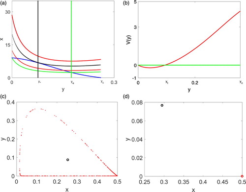We use Figure 1(a) to illustrate Theorem 2.1 with $\lambda =10$ and $\alpha =30$. Then $2\alpha -\left(3\lambda -1\right)/\left(\lambda -1\right)\approx 56.8>0$. The two isoclines are tangent to each other at $\beta ={\beta }_{\ast }\approx 0.0507$, and there is a unique positive intersection when $\beta =1/\overline{x}\approx 0.111$. It is clear that the system has two interior steady states if β is in $(0.0507,0.111)$ while there is a unique interior steady state if $\beta >0.111$ and there is no interior steady state if $\beta <{\beta }_{\ast }=0.0507$.

Figure 1. (a) plots isoclines with four β values to demonstrate Theorem 2.1. (b) provides a graph of $V\left(y\right)$ to illustrate Lemma 2.3. (c) and (d) plot solutions for the case where $y_d<y_t=y_{\ast }$ by removing the first 8000 iterations and plot the next 5000 iterations. In (c), β is chosen larger than $1/\overline{x}$ so that there is a unique interior steady state which is a repeller. In (d), β is smaller than $1/\overline{x}$ but larger than ${\beta }_{\ast }$ so that there are two interior steady states and the boundary steady state $E_1=(\overline{x},0)=(0.5,0)$ is asymptotically stable. The solution converges to the boundary steady state $E_1$.

Once existence and the number of interior steady states are determined, we proceed to review notations relative to the study of local stability of the steady states. With fixed $\lambda >1$, Theorem 2.1 means that any point $(x,y)$ on $x=f\left(y\right)$ with $0<y<y_c$ will be an interior steady state for a certain β. Using $x=f\left(y\right)$ we can rewrite $\det \left(J\right)$ and $tr\left(J\right)$ of the Jacobian matrix as functions of y, (13) $J=\left(\begin{array}{cc}\frac{1}{\lambda e^{-\mathrm{♢}}}& -f\left(y\right)(1+2\alpha y)\\ \frac{y}{f\left(y\right)}& \frac{y(1+2\alpha y)e^{-\mathrm{♢}}}{1-e^{-\mathrm{♢}}}\end{array}\right).$(13) Since $\mathrm{tr}\left(J\right)>0$ on $[0,y_c)$ and by the Jury condition, we need only to study $det\left(J\right)$ and (14) $V\left(y\right):=1+det\left(J\right)-tr\left(J\right)$(14) in order to determine local stability of $(x,y)$ on $x=f\left(y\right)$. By a straightforward calculation, we verified the following in [4].

Lemma 2.2

Let $\lambda >1$. Then $\left(\mathrm{d}/\mathrm{d}y\right)\det \left(J\right(y\left)\right)>0$ on $(0,y_c)$ with $\det \left(J\right(0^{+}\left)\right)=1/\lambda <1$ and $\det \left(J\right(y_c^{-}\left)\right)\ge \lambda \ln \lambda /\left(\lambda -1\right)>1$. Hence, there exists a unique $y_d\in (0,y_c)$ such that $\det \left(J\right(y_d\left)\right)=1$.

As a result of Lemma 2.2, $\det \left(J\right(y\left)\right)<1$ for $y\in (0,y_d)$ and $\det \left(J\right(y\left)\right)>1$ for $y\in (y_d,y_c)$. For the other inequality in the Jury condition, it is shown in [4] that $V\left(y\right)$ satisfies the following.

Lemma 2.3

Let $\lambda >1$ and $2\alpha >\left(3\lambda -1\right)/\left(\lambda -1\right)$. Then $V\left(y\right)$ has a unique zero at $y=y_t$ with $y_t<2\lambda /\left(\lambda +1\right)$, where $V\left(y\right)<0$ on $(0,y_t)$ and $V\left(y\right)>0$ on $(y_t,y_c)$.

It follows from Lemma 2.3 that $\mathrm{tr}\left(J\right(y\left)\right)>1+\det \left(J\right(y\left)\right)$ for $y\in (0,y_t)$ while $\mathrm{tr}\left(J\right(y\left)\right)<1+\det \left(J\right(y\left)\right)$ if $y\in (y_t,y_c)$. To illustrate the lemma, Figure 1(b) presents the graph $V\left(y\right)$ with $\lambda =10$, $\beta =3$, and $\alpha =15$ for which $2\alpha >\left(3\lambda -1\right)/\left(\lambda -1\right)$ holds. It indicates that there exists a unique $y_t$ in $(0,y_c)$ for which $V\left(y\right)=0$.

3. Main results

In the previous section, we have briefly introduced four critical points $y_{\ast },y_e,y_d$ and $y_t$ in $(0,y_c)$. In this section, we will investigate their order relations from which local stability of an interior steady state $(x,y)$ can be determined directly. For instance, Jury condition and Lemmas 2.2 and 2.3 imply $(x,y)$ is asymptotically stable if $y\in (y_t,y_d)$, which makes sense only if $y_t<y_d$.

We will first prove in Section 3.1 that $y_{\ast }=y_t$. The comparison between $y_t$ and $y_d$ is given in Section 3.2 and the order of $y_d$ and $y_e$ is studied in Section 3.3. Local stability of the interior steady states is presented in Section 3.4. These proofs depend heavily on Lemmas 2.2 and 2.3. However, the technique explored in this investigation is very different from that employed in Chow et al. [4].

3.1. The proof of $y_{\ast }=y_t$

We will prove that at the tangency of the two isoclines, one of the inequalities in the Jury condition is an equality, that is, $\mathrm{tr}\left(J\right(y_{\ast }\left)\right)=1+\det \left(J\right(y_{\ast }\left)\right)$. As a consequence, $y_{\ast }=y_t$ by Lemma 2.3. To simplify the analysis, we perform changes of variables. To this end, we define new variables t and s (15) $t=y(1+2\alpha y)\text{and}s=e^{\diamond }\text{for }y\in (0,y_c),$(15) where $\diamond =y(1+\alpha y)$ by (5(5) $\mathrm{♢}=y(1+\alpha y).$(5) ). Clearly, both t and s are strictly increasing functions of y. Since $y(1+\alpha y)=\ln s$, we obtain (16) $y=\frac{-1+\sqrt{1+4\alpha \ln s}}{2\alpha }=\frac{2\ln s}{1+\sqrt{1+4\alpha \ln s}}\text{for }s\in [1,\lambda ].$(16) Note that $e^{y_c(1+\alpha y_c)}=\lambda$. By (15(15) $t=y(1+2\alpha y)\text{and}s=e^{\diamond }\text{for }y\in (0,y_c),$(15) ), $t\left(s\right)=2y(1+\alpha y)-y$. Hence, (17) $t\left(s\right)=2\ln s+\frac{1-\sqrt{1+4\alpha \ln s}}{2\alpha }=2\ln s\left(1-\frac{1}{1+\sqrt{1+4\alpha \ln s}}\right).$(17) In the following, we regard s as the variable. By (4(4) $x=h\left(y\right):=\frac{y}{\beta (1-e^{-y(1+\alpha y)})}>0\text{with }h\left(0\right)=\frac{1}{\beta }\text{ and }h\left(\mathrm{\infty }\right)=\mathrm{\infty }.$(4) ) and (7(7) $x=f\left(y\right):=\lambda e^{-y(1+\alpha y)}-1$(7) ), (18) $f\left(y\right)=\frac{\lambda -s}{s}\text{and}h\left(y\right)=\frac{ys}{\beta (s-1)}.$(18) Since $f^{\mathrm{\prime }}\left(y\right)=-\lambda e^{-\diamond }(1+2\alpha y)/1=-\lambda t/ys$ and $h^{\mathrm{\prime }}\left(y\right)=e^{\diamond }(e^{\diamond }-1-y(1+2\alpha y\left)\right)/\beta (e^{\diamond }-1{)}^2=s(s-1-t)/\beta (s-1{)}^2$, the two equations in (10(10) $\begin{array}{rl}f\left(y\right)& =h\left(y\right)\\ f^{\mathrm{\prime }}\left(y\right)& =h^{\mathrm{\prime }}\left(y\right).\end{array}$(10) ) for which $y_{\ast }$ is defined are equivalent to $\beta =s^{2}y/(s-1)(\lambda -s)$ and $\beta =-s^{2}y(s-1-t)/\lambda t(s-1{)}^2$, respectively. Cancelling β, we obtain (19) $t\left(s\right)=g\left(s\right):=\frac{(s-1)(s-\lambda )}{(\lambda +1)s-2\lambda }\text{at }s=e^{y_{\ast }(1+\alpha y_{\ast })}.$(19) Note that by definition, g<0 on $(2\lambda /\lambda +1,\lambda ]$ and $g^{\mathrm{\prime }}\left(s\right)=\frac{1}{\lambda +1}+\frac{\lambda (\lambda -1{)}^2}{(\lambda +1)(2\lambda -(\lambda +1)s{)}^2}>0,g^{\mathrm{\prime \prime }}\left(s\right)=\frac{2\lambda (\lambda -1{)}^2}{(2\lambda -(\lambda +1)s{)}^3}>0.$ Hence (20) $g\left(1\right)=0,g^{\mathrm{\prime }}\left(1\right)=1,g^{\mathrm{\prime \prime }}\left(1\right)=\frac{2\lambda }{\lambda -1}\text{and}g{\uparrow }_0^{\mathrm{\infty }}\text{on }\left[1,\frac{2\lambda }{\lambda +1}\right).$(20) On the other hand, we have from (13(13) $J=\left(\begin{array}{cc}\frac{1}{\lambda e^{-\mathrm{♢}}}& -f\left(y\right)(1+2\alpha y)\\ \frac{y}{f\left(y\right)}& \frac{y(1+2\alpha y)e^{-\mathrm{♢}}}{1-e^{-\mathrm{♢}}}\end{array}\right).$(13) ) that in terms of s, (21) $\det \left(J\right)=\left(\frac{1}{\lambda (1-e^{-\diamond })}+1\right)y(1+2\alpha y)=\left(\frac{s}{\lambda (s-1)}+1\right)t$(21) and (22) $\mathrm{tr}\left(J\right)=\frac{1}{\lambda e^{-\diamond }}+\frac{e^{-\diamond }}{1-e^{-\diamond }}y(1+2\alpha y)=\frac{s}{\lambda }+\frac{t}{s-1}.$(22) Using (19(19) $t\left(s\right)=g\left(s\right):=\frac{(s-1)(s-\lambda )}{(\lambda +1)s-2\lambda }\text{at }s=e^{y_{\ast }(1+\alpha y_{\ast })}.$(19) ) and (21(21) $\det \left(J\right)=\left(\frac{1}{\lambda (1-e^{-\diamond })}+1\right)y(1+2\alpha y)=\left(\frac{s}{\lambda (s-1)}+1\right)t$(21) ), a simple calculation shows that (23) $V\left(y\right)=0\text{if and only if }t\left(s\right)=\frac{(s-1)(s-\lambda )}{(\lambda +1)s-2\lambda }=g\left(s\right),$(23) as defined in (22(22) $\mathrm{tr}\left(J\right)=\frac{1}{\lambda e^{-\diamond }}+\frac{e^{-\diamond }}{1-e^{-\diamond }}y(1+2\alpha y)=\frac{s}{\lambda }+\frac{t}{s-1}.$(22) ). Then it follows from Lemma 2.3 that (24) $\{s\in (1,\lambda ):t(s)=g(s\left)\right\}=\left\{e^{y_t(1+\alpha y_t)}\right\}.$(24) Since $0<e^{y_{\ast }(1+\alpha y_{\ast })}<e^{y_c(1+\alpha y_c)}<\lambda$, (19(19) $t\left(s\right)=g\left(s\right):=\frac{(s-1)(s-\lambda )}{(\lambda +1)s-2\lambda }\text{at }s=e^{y_{\ast }(1+\alpha y_{\ast })}.$(19) ) and (24(24) $\{s\in (1,\lambda ):t(s)=g(s\left)\right\}=\left\{e^{y_t(1+\alpha y_t)}\right\}.$(24) ) imply the following.

Proposition 3.1

Let $\lambda >1$ and $2\alpha >\left(3\lambda -1\right)/\left(\lambda -1\right)$. Then $e^{y_{\ast }(1+\alpha y_{\ast })}=e^{y_t(1+\alpha y_t)}$. That is, $y_{\ast }=y_t$.

3.2. Comparison between $y_d$ and $y_{\ast }$

In this subsection, we will compare $y_d$ with $y_{\ast }$. By Proposition 3.1 and (11(11) $0<y_1^{\ast }<y_{\ast }<y_2^{\ast }<y_e\le y^{\ast }<y_c.$(11) ), (25) $\text{if }{y}_d\le y_{\ast },\text{then }{y}_d\le y_{\ast }=y_t<y_e.$(25) Using Lemmas 2.2 and 2.3, we can then determine immediately the local stability of any interior steady states. To this effort, we take the advantage of the new variable s defined in Section 3.1.

Define (26) $f_d\left(s\right):=\frac{\lambda (s-1)}{(\lambda +1)s-\lambda }\text{on }[1,\mathrm{\infty }).$(26) It is easy to check that on $[1,\mathrm{\infty })$, (27) $f_d^{\mathrm{\prime }}\left(s\right)=\frac{\lambda }{\left(\right(\lambda +1)s-\lambda {)}^2}>0\text{and}{f}_d^{\mathrm{\prime \prime }}\left(s\right)=\frac{-2\lambda (\lambda +1)}{\left(\right(\lambda +1)s-\lambda {)}^3}<0.$(27) In particular, $f_d\left(s\right)$ is strictly increasing and concave on $[1,\mathrm{\infty })$. Moreover, (28) $f_d\left(1\right)=0,f_d\left(\mathrm{\infty }\right)=\frac{\lambda }{\lambda +1}\text{ and }{f}_d^{\mathrm{\prime }}\left(1\right)=\lambda .$(28) By Lemma 2.2 and (21(21) $\det \left(J\right)=\left(\frac{1}{\lambda (1-e^{-\diamond })}+1\right)y(1+2\alpha y)=\left(\frac{s}{\lambda (s-1)}+1\right)t$(21) ), (29) $\{s\in (1,\lambda ]:t(s)=f_d(s\left)\right\}=\left\{e^{y_d(1+\alpha y_d)}\right\}.$(29) For $\lambda >1$, a straightforward calculation shows that (30) $1<{\lambda }_{\ast }=:\frac{2{\lambda }^2+3\lambda -\lambda \sqrt{4{\lambda }^2-3}}{2(\lambda +1)}<\frac{2\lambda }{\lambda +1}<\lambda .$(30) Using (19(19) $t\left(s\right)=g\left(s\right):=\frac{(s-1)(s-\lambda )}{(\lambda +1)s-2\lambda }\text{at }s=e^{y_{\ast }(1+\alpha y_{\ast })}.$(19) ), $f_d\left(s\right)=g\left(s\right)$ if and only if $(s-1)\left(\right(\lambda +1)s^2-(2{\lambda }^2+3\lambda )s+3{\lambda }^2)=0$. Hence (31) $\{s\in [1,\lambda ]:f_d(s)=g(s\left)\right\}=\{1,{\lambda }_{\ast }\}$(31) as the third root $\left(2{\lambda }^2+3\lambda +\lambda \sqrt{4{\lambda }^2-3}\right)/2(\lambda +1)>\lambda$.

We now prove that the order between $y_d$ and $y_{\ast }$ is equivalent to the order between $f_d\left({\lambda }_{\ast }\right)$ and $t\left({\lambda }_{\ast }\right)$.

Theorem 3.2

Let $\lambda >1$ and $2\alpha >\left(3\lambda -1\right)/\left(\lambda -1\right)$. Then $f_d\left({\lambda }_{\ast }\right)⊳t\left({\lambda }_{\ast }\right)$ if and only if $y_d⊳y_{\ast }$. Here $⊳$ can be either <,= or >.

Proof.

By (17(17) $t\left(s\right)=2\ln s+\frac{1-\sqrt{1+4\alpha \ln s}}{2\alpha }=2\ln s\left(1-\frac{1}{1+\sqrt{1+4\alpha \ln s}}\right).$(17) ), (20(20) $g\left(1\right)=0,g^{\mathrm{\prime }}\left(1\right)=1,g^{\mathrm{\prime \prime }}\left(1\right)=\frac{2\lambda }{\lambda -1}\text{and}g{\uparrow }_0^{\mathrm{\infty }}\text{on }\left[1,\frac{2\lambda }{\lambda +1}\right).$(20) ) and (28(28) $f_d\left(1\right)=0,f_d\left(\mathrm{\infty }\right)=\frac{\lambda }{\lambda +1}\text{ and }{f}_d^{\mathrm{\prime }}\left(1\right)=\lambda .$(28) ), $f_d\left(1\right)=t\left(1\right)=g\left(1\right)=0$. We claim (32) $f_d\left(s\right)>t\left(s\right)>g\left(s\right)\text{on a small interval }(1,1+\delta ).$(32) Since $t^{\mathrm{\prime }}\left(s\right)=\left(1/s\right)(2-1/\sqrt{1+4\alpha \ln s})$ and $t^{\mathrm{\prime \prime }}\left(s\right)=\left(1/s^2\right)\left(\right(2\alpha +(1+4\alpha \ln s)\left)/\right(1+4\alpha \ln s{)}^{3/2}-2)$, we have (33) $t^{\mathrm{\prime }}\left(1\right)=1\text{and}{t}^{\mathrm{\prime \prime }}\left(1\right)=2\alpha -1.$(33) The first inequality in (32(32) $f_d\left(s\right)>t\left(s\right)>g\left(s\right)\text{on a small interval }(1,1+\delta ).$(32) ) is due to $f_d^{\mathrm{\prime }}\left(1\right)=\lambda >1=t^{\mathrm{\prime }}\left(1\right)$. Using (20(20) $g\left(1\right)=0,g^{\mathrm{\prime }}\left(1\right)=1,g^{\mathrm{\prime \prime }}\left(1\right)=\frac{2\lambda }{\lambda -1}\text{and}g{\uparrow }_0^{\mathrm{\infty }}\text{on }\left[1,\frac{2\lambda }{\lambda +1}\right).$(20) ), (33(33) $t^{\mathrm{\prime }}\left(1\right)=1\text{and}{t}^{\mathrm{\prime \prime }}\left(1\right)=2\alpha -1.$(33) ) and the assumption $2\alpha >\left(3\lambda -1\right)/\left(\lambda -1\right)$, the second inequality follows from $t^{\mathrm{\prime }}\left(1\right)-g^{\mathrm{\prime }}\left(1\right)=0$ and $t^{\mathrm{\prime \prime }}\left(1\right)-g^{\mathrm{\prime \prime }}\left(1\right)=2\alpha -\left(3\lambda -1\right)/\left(\lambda -1\right)>0$. Recall $f_d\left({\lambda }_{\ast }\right)=g\left({\lambda }_{\ast }\right)$ by (31(31) $\{s\in [1,\lambda ]:f_d(s)=g(s\left)\right\}=\{1,{\lambda }_{\ast }\}$(31) ). Together with (32(32) $f_d\left(s\right)>t\left(s\right)>g\left(s\right)\text{on a small interval }(1,1+\delta ).$(32) ), we have (34) $f_d\left(s\right)>g\left(s\right)\text{for }s\in (1,{\lambda }_{\ast })\text{and}{f}_d\left({\lambda }_{\ast }\right)=g\left({\lambda }_{\ast }\right).$(34) If $f_d\left({\lambda }_{\ast }\right)<t\left({\lambda }_{\ast }\right)$, then $f_d\left(\underset{\_}{s}\right)=t\left(\underset{\_}{s}\right)$ for some $\underset{\_}{s}\in (1,{\lambda }_{\ast })$ by (32(32) $f_d\left(s\right)>t\left(s\right)>g\left(s\right)\text{on a small interval }(1,1+\delta ).$(32) ) and $t\left(\overline{s}\right)=g\left(\overline{s}\right)$ for some $\overline{s}\in ({\lambda }_{\ast },2\lambda /\lambda +1)$ as $g\left(2\lambda /{\lambda +1}^{-}\right)=\mathrm{\infty }$. By (24(24) $\{s\in (1,\lambda ):t(s)=g(s\left)\right\}=\left\{e^{y_t(1+\alpha y_t)}\right\}.$(24) ) and (29(29) $\{s\in (1,\lambda ]:t(s)=f_d(s\left)\right\}=\left\{e^{y_d(1+\alpha y_d)}\right\}.$(29) ) and Proposition 3.1, $e^{y_d(1+\alpha y_d)}=\underset{\_}{s}<{\lambda }_{\ast }<\overline{s}=e^{y_{\ast }(1+\alpha y_{\ast })}\text{and thus }{y}_d<y_{\ast }.$ Similarly, $f_d\left({\lambda }_{\ast }\right)>t\left({\lambda }_{\ast }\right)$ implies $t\left(\underset{\_}{s}\right)=g\left(\underset{\_}{s}\right)$ for some $\underset{\_}{s}\in (1,{\lambda }_{\ast })$ by (32(32) $f_d\left(s\right)>t\left(s\right)>g\left(s\right)\text{on a small interval }(1,1+\delta ).$(32) ) and $f_d\left(\overline{s}\right)=t\left(\overline{s}\right)$ for some $\overline{s}>{\lambda }_{\ast }$ as $f_d\left(\mathrm{\infty }\right)=\lambda /\left(\lambda +1\right)<t\left(\mathrm{\infty }\right)=\mathrm{\infty }$. Using (24(24) $\{s\in (1,\lambda ):t(s)=g(s\left)\right\}=\left\{e^{y_t(1+\alpha y_t)}\right\}.$(24) ) and (29(29) $\{s\in (1,\lambda ]:t(s)=f_d(s\left)\right\}=\left\{e^{y_d(1+\alpha y_d)}\right\}.$(29) ) again, $e^{y_{\ast }(1+\alpha y_{\ast })}=\underset{\_}{s}<{\lambda }_{\ast }<\overline{s}=e^{y_d(1+\alpha y_d)}\text{and thus }{y}_{\ast }<y_d.$ The remaining case means $f_d\left({\lambda }_{\ast }\right)=t\left({\lambda }_{\ast }\right)=g\left({\lambda }_{\ast }\right)$. By the same reasoning, $e^{y_{\ast }(1+\alpha y_{\ast })}={\lambda }_{\ast }=e^{y_d(1+\alpha y_d)}$ and hence $y_{\ast }=y_d$ is shown.

Computer simulation indicates that both $y_d<y_{\ast }$ and $y_{\ast }<y_d$ can occur. Under the restriction of $2\alpha >\left(3\lambda -1\right)/\left(\lambda -1\right)$, i.e. $\lambda >\left(2\alpha -1\right)/\left(2\alpha -3\right)>1$, numerical simulations suggest the following possible facts, namely $\{\lambda :f_d({\lambda }_{\ast })<t({\lambda }_{\ast }\left)\right\}=\mathrm{\varnothing }$ when α is small, $\{\lambda :f_d({\lambda }_{\ast })<t({\lambda }_{\ast }\left)\right\}$ is an interval away from 1 when α increases up to 11, and $\{\lambda :f_d({\lambda }_{\ast })<t({\lambda }_{\ast }\left)\right\}=(1,c)$ when α exceeds 68. In all cases, the set $\{\lambda :f_d({\lambda }_{\ast })<t({\lambda }_{\ast }\left)\right\}$ seems to be bounded and hence $\{\lambda :f_d({\lambda }_{\ast })>t({\lambda }_{\ast }\left)\right\}$ is unbounded. This observation is confirmed as follows.

Corollary 3.3

Let $\lambda >1$ and $2\alpha >\left(3\lambda -1\right)/\left(\lambda -1\right)$. Then $y_{\ast }<y_d$ holds for λ large.

Proof.

By Theorem 3.2, it is sufficient to prove $f_d\left({\lambda }_{\ast }\right)>t\left({\lambda }_{\ast }\right)$ for all large λ. Since $\underset{\lambda \to \mathrm{\infty }}{lim}{\lambda }_{\ast }=\frac{3}{2}$, $f_d\left({\lambda }_{\ast }\right)=\lambda ({\lambda }_{\ast }-1)/\left((\lambda +1){\lambda }_{\ast }-\lambda \right)\to 1$ as $\lambda \to \mathrm{\infty }$. By (17(17) $t\left(s\right)=2\ln s+\frac{1-\sqrt{1+4\alpha \ln s}}{2\alpha }=2\ln s\left(1-\frac{1}{1+\sqrt{1+4\alpha \ln s}}\right).$(17) ), $t\left(s\right)\le 2\ln s$. Hence $\underset{\lambda \to \mathrm{\infty }}{lim}t\left({\lambda }_{\ast }\right)=t\left(\frac{3}{2}\right)\le 2\ln \left(1.5\right)\approx 0.811<1$. That is, $f_d\left({\lambda }_{\ast }\right)>t\left({\lambda }_{\ast }\right)$ holds for λ large enough. The claim is proven.

3.3. Comparison between $y_d$ and $y_e$

In contrast to (25(25) $\text{if }{y}_d\le y_{\ast },\text{then }{y}_d\le y_{\ast }=y_t<y_e.$(25) ), $\text{if }{y}_{\ast }<y_d,\text{then either }{y}_{\ast }=y_t<y_d<y_e\text{ or }{y}_{\ast }=y_t<y_e\le y_d.$ So we need to compare $y_d$ with $y_e$ before using Lemmas 2.2 and 2.3 to determine local stability of any interior steady states. We shall mimic the method used in the proof of Theorem 3.2. For $s\ge 1$, define (35) $\tilde{g}\left(s\right)=2\ln s+\frac{(s-1)(s-\lambda )}{(\lambda -1)s^2}=2\ln s+\frac{1}{\lambda -1}-\frac{\lambda +1}{(\lambda -1)s}+\frac{\lambda }{(\lambda -1)s^2}.$(35) Hence, ${\tilde{g}}^{\mathrm{\prime }}\left(s\right)=\frac{2}{/}s+\left(\lambda +1\right)/(\lambda -1)s^2-2\lambda /(\lambda -1)s^3$ and (36) ${\tilde{g}}^{\mathrm{\prime \prime }}\left(s\right)=\frac{-2(\lambda -1)s^2-2(\lambda +1)s+6\lambda }{(\lambda -1)s^4}.$(36) Moreover, (37) $\tilde{g}\left(1\right)=0,{\tilde{g}}^{\mathrm{\prime }}\left(1\right)=1\text{and}{\tilde{g}}^{\mathrm{\prime \prime }}\left(1\right)=\frac{2\lambda }{\lambda -1}.$(37) Note that by (17(17) $t\left(s\right)=2\ln s+\frac{1-\sqrt{1+4\alpha \ln s}}{2\alpha }=2\ln s\left(1-\frac{1}{1+\sqrt{1+4\alpha \ln s}}\right).$(17) ), (38) $t\left(s\right)<2\ln s<\tilde{g}\left(s\right)\text{on }(\lambda ,\mathrm{\infty }).$(38) We claim that (39) $\{s\in (1,\mathrm{\infty }):t(s)=\tilde{g}(s\left)\right\}=\left\{e^{y_e(1+\alpha y_e)}\right\}.$(39) Recall that $E^{\ast }=(x_e,y_e)$ is the unique interior steady state when $\beta =1/\overline{x}=1/\left(\lambda -1\right)$. That means $y_e$ is the unique positive solution to $h\left(y\right)=f\left(y\right)$ when $\beta =1/\left(\lambda -1\right)$. Using (18(18) $f\left(y\right)=\frac{\lambda -s}{s}\text{and}h\left(y\right)=\frac{ys}{\beta (s-1)}.$(18) ) and (16(16) $y=\frac{-1+\sqrt{1+4\alpha \ln s}}{2\alpha }=\frac{2\ln s}{1+\sqrt{1+4\alpha \ln s}}\text{for }s\in [1,\lambda ].$(16) ), we get $\left\{s\in (1,\mathrm{\infty }):\frac{-2\ln s}{1+\sqrt{1+4\alpha \ln s}}=\frac{(s-1)(s-\lambda )}{(\lambda -1)s^2}\right\}=\left\{e^{y_e(1+\alpha y_e)}\right\}.$ Adding $2\ln s$ to both sides of the equation above, (39(39) $\{s\in (1,\mathrm{\infty }):t(s)=\tilde{g}(s\left)\right\}=\left\{e^{y_e(1+\alpha y_e)}\right\}.$(39) ) follows from (17(17) $t\left(s\right)=2\ln s+\frac{1-\sqrt{1+4\alpha \ln s}}{2\alpha }=2\ln s\left(1-\frac{1}{1+\sqrt{1+4\alpha \ln s}}\right).$(17) ) and (35(35) $\tilde{g}\left(s\right)=2\ln s+\frac{(s-1)(s-\lambda )}{(\lambda -1)s^2}=2\ln s+\frac{1}{\lambda -1}-\frac{\lambda +1}{(\lambda -1)s}+\frac{\lambda }{(\lambda -1)s^2}.$(35) ).

By (20(20) $g\left(1\right)=0,g^{\mathrm{\prime }}\left(1\right)=1,g^{\mathrm{\prime \prime }}\left(1\right)=\frac{2\lambda }{\lambda -1}\text{and}g{\uparrow }_0^{\mathrm{\infty }}\text{on }\left[1,\frac{2\lambda }{\lambda +1}\right).$(20) ) and (37(37) $\tilde{g}\left(1\right)=0,{\tilde{g}}^{\mathrm{\prime }}\left(1\right)=1\text{and}{\tilde{g}}^{\mathrm{\prime \prime }}\left(1\right)=\frac{2\lambda }{\lambda -1}.$(37) ), $\tilde{g}\left(1\right)=g\left(1\right)=0$, ${\tilde{g}}^{\mathrm{\prime }}\left(1\right)=g^{\mathrm{\prime }}\left(1\right)$ and ${\tilde{g}}^{\mathrm{\prime \prime }}\left(1\right)=g^{\mathrm{\prime \prime }}\left(1\right)$. Similar to (32(32) $f_d\left(s\right)>t\left(s\right)>g\left(s\right)\text{on a small interval }(1,1+\delta ).$(32) ) we can show that (40) $f_d\left(s\right)>t\left(s\right)>\tilde{g}\left(s\right)\text{on a small interval }(1,1+\tilde{\delta }).$(40) Since $f_d\left(\mathrm{\infty }\right)=\lambda /\left(\lambda +1\right)<\mathrm{\infty }=\tilde{g}\left(\mathrm{\infty }\right)$, (40(40) $f_d\left(s\right)>t\left(s\right)>\tilde{g}\left(s\right)\text{on a small interval }(1,1+\tilde{\delta }).$(40) ) implies that $f_d\left(s\right)=\tilde{g}\left(s\right)$ must have a solution on $(1,\mathrm{\infty })$. Let (41) ${\tilde{\lambda }}_{\ast }=\text{ min }\{s>1:f_d(s)=\tilde{g}(s\left)\right\}.$(41) Note that ${\tilde{\lambda }}_{\ast }$ depends only on λ. Therefore similar to (34(34) $f_d\left(s\right)>g\left(s\right)\text{for }s\in (1,{\lambda }_{\ast })\text{and}{f}_d\left({\lambda }_{\ast }\right)=g\left({\lambda }_{\ast }\right).$(34) ), we have $f_d\left(s\right)>\tilde{g}\left(s\right)\text{on }(1,{\tilde{\lambda }}_{\ast })\text{and}{f}_d\left({\lambda }_{\ast }\right)=\tilde{g}\left({\lambda }_{\ast }\right).$ Using (38(38) $t\left(s\right)<2\ln s<\tilde{g}\left(s\right)\text{on }(\lambda ,\mathrm{\infty }).$(38) ) and with the replacement of (24(24) $\{s\in (1,\lambda ):t(s)=g(s\left)\right\}=\left\{e^{y_t(1+\alpha y_t)}\right\}.$(24) ) by (39(39) $\{s\in (1,\mathrm{\infty }):t(s)=\tilde{g}(s\left)\right\}=\left\{e^{y_e(1+\alpha y_e)}\right\}.$(39) ), we can repeat the same arguments as in Theorem 3.2 to obtain the following result.

Theorem 3.4

Let $\lambda >1$ and $2\alpha >\left(3\lambda -1\right)/\left(\lambda -1\right)$. Then $f_d\left({\tilde{\lambda }}_{\ast }\right)⊳t\left({\tilde{\lambda }}_{\ast }\right)$ if and only if $y_d⊳y_e$. Here $⊳$ can be $<,=$ or >.

Computer simulation indicates that both $y_d>y_e$ and $y_d<y_e$ can happen depending on parameter regimes, which will be shown theoretically as follows.

Define $H\left(s\right)=2\ln s-\left(s-1\right)/s^2$ on $[1,\mathrm{\infty })$. It is easy to verify that $H\left(s\right)$ increases strictly with $H\left(1\right)=0$ and $H\left(\mathrm{\infty }\right)=\mathrm{\infty }$. Hence, (42) $H\left(s\right)=1\text{ has a unique solution }\eta \text{ on }[1,\mathrm{\infty }).$(42) Note that $\eta \approx 1.867$ by computer calculation.

Corollary 3.5

Let $\lambda >1$ and $2\alpha >\left(3\lambda -1\right)/\left(\lambda -1\right)$. Then $y_d\gtrless y_e$ for λ large if $\alpha \lessgtr ({\eta }^2-\eta +1){\eta }^2/2(\eta -1{)}^2\approx 6.071$.

Proof.

Since ${\tilde{\lambda }}_{\ast }$ is not explicitly given as ${\lambda }_{\ast }$ in (30(30) $1<{\lambda }_{\ast }=:\frac{2{\lambda }^2+3\lambda -\lambda \sqrt{4{\lambda }^2-3}}{2(\lambda +1)}<\frac{2\lambda }{\lambda +1}<\lambda .$(30) ), it is not clear at the first sight whether $\underset{\lambda \to \mathrm{\infty }}{lim}{\tilde{\lambda }}_{\ast }$ exists. We claim that (43) $1.1<{\tilde{\lambda }}_{\ast }<2\text{for }\lambda >3.$(43) Assume (43(43) $1.1<{\tilde{\lambda }}_{\ast }<2\text{for }\lambda >3.$(43) ) is true temporarily. By (43(43) $1.1<{\tilde{\lambda }}_{\ast }<2\text{for }\lambda >3.$(43) ), $f_d\left({\tilde{\lambda }}_{\ast }\right)=\lambda ({\tilde{\lambda }}_{\ast }-1)/(\lambda +1){\tilde{\lambda }}_{\ast }-\lambda \to 1$ as $\lambda \to \mathrm{\infty }$. Letting $\lambda \to \mathrm{\infty }$ in $f_d\left({\tilde{\lambda }}_{\ast }\right)=\tilde{g}\left({\tilde{\lambda }}_{\ast }\right)$, we obtain from (35(35) $\tilde{g}\left(s\right)=2\ln s+\frac{(s-1)(s-\lambda )}{(\lambda -1)s^2}=2\ln s+\frac{1}{\lambda -1}-\frac{\lambda +1}{(\lambda -1)s}+\frac{\lambda }{(\lambda -1)s^2}.$(35) ) that $1=2\ln s-\frac{s-1}{s^2}=H\left(s\right)$ holds for both $s=lim inf{\tilde{\lambda }}_{\ast }$ and $s=lim sup{\tilde{\lambda }}_{\ast }$. Using (42(42) $H\left(s\right)=1\text{ has a unique solution }\eta \text{ on }[1,\mathrm{\infty }).$(42) ), (44) $\underset{\lambda \to \mathrm{\infty }}{lim}{\tilde{\lambda }}_{\ast }=\eta .$(44) Define $A=\underset{\lambda \to \mathrm{\infty }}{lim}\left(f_d\right({\tilde{\lambda }}_{\ast })-t({\tilde{\lambda }}_{\ast }\left)\right)$. Then $A\gtrless 0$ means $f_d\left({\tilde{\lambda }}_{\ast }\right)\gtrless t\left({\tilde{\lambda }}_{\ast }\right)$ for λ large. By (17(17) $t\left(s\right)=2\ln s+\frac{1-\sqrt{1+4\alpha \ln s}}{2\alpha }=2\ln s\left(1-\frac{1}{1+\sqrt{1+4\alpha \ln s}}\right).$(17) ), (44(44) $\underset{\lambda \to \mathrm{\infty }}{lim}{\tilde{\lambda }}_{\ast }=\eta .$(44) ) and (42(42) $H\left(s\right)=1\text{ has a unique solution }\eta \text{ on }[1,\mathrm{\infty }).$(42) ), $A=1-2\ln \eta -\frac{1-\sqrt{1+4\alpha \ln \eta }}{2\alpha }=\frac{2\ln \eta }{\sqrt{1+4\alpha \ln \eta }+1}-\frac{\eta -1}{{\eta }^2}.$ A simple calculation shows $A\gtrless 0\text{if and only if }\alpha \lessgtr \frac{({\eta }^2-\eta +1){\eta }^2}{2(\eta -1{)}^2}\approx \mathrm{6.071.}$ The conclusion then follows from Theorem 3.4.

It remains to verify (43(43) $1.1<{\tilde{\lambda }}_{\ast }<2\text{for }\lambda >3.$(43) ). By (27(27) $f_d^{\mathrm{\prime }}\left(s\right)=\frac{\lambda }{\left(\right(\lambda +1)s-\lambda {)}^2}>0\text{and}{f}_d^{\mathrm{\prime \prime }}\left(s\right)=\frac{-2\lambda (\lambda +1)}{\left(\right(\lambda +1)s-\lambda {)}^3}<0.$(27) ), $f_d\left(s\right)$ is concave on $(1,\mathrm{\infty })$. By (36(36) ${\tilde{g}}^{\mathrm{\prime \prime }}\left(s\right)=\frac{-2(\lambda -1)s^2-2(\lambda +1)s+6\lambda }{(\lambda -1)s^4}.$(36) ), it is easy to check that ${\tilde{g}}^{\mathrm{\prime \prime }}\left(s\right)>0$ for $s\in (1,1.1)$. That means $\tilde{g}\left(s\right)$ is convex on the interval $(1,1.1)$. Using $f_d\left(1\right)=\tilde{g}\left(1\right)=0$ and for $\lambda >3$, $f_d\left(1.1\right)=\frac{0.1\lambda }{0.1\lambda +1.1}>\frac{1}{5}>0.1960\approx 2\ln 1.1>\tilde{g}\left(1.1\right),$ we see that $f_d\left(s\right)>\tilde{g}\left(s\right)$ for $s\in (1,1.1)$. Hence $1.1<{\tilde{\lambda }}_{\ast }$ by the definition (41(41) ${\tilde{\lambda }}_{\ast }=\text{ min }\{s>1:f_d(s)=\tilde{g}(s\left)\right\}.$(41) ). For $\lambda >2$, $\tilde{g}\left(2\right)=2\ln 2-\frac{\lambda -2}{4(\lambda -1)}>2\ln 2-\frac{1}{4}\approx 1.13>1>\frac{\lambda }{\lambda +2}=f_d\left(2\right).$ Therefore, (41(41) ${\tilde{\lambda }}_{\ast }=\text{ min }\{s>1:f_d(s)=\tilde{g}(s\left)\right\}.$(41) ) implies ${\tilde{\lambda }}_{\ast }<2$. The claim (43(43) $1.1<{\tilde{\lambda }}_{\ast }<2\text{for }\lambda >3.$(43) ) is verified and the proof is complete.

3.4. Local stability of the interior steady states

In this subsection, we provide local stability of the interior steady states. Recall from Theorem 3.2 that there are two interior steady states $E_1^{\ast }=(x_1^{\ast },y_1^{\ast })$ and $E_2^{\ast }=(x_2^{\ast },y_2^{\ast })$ where $y_1^{\ast }<y_2^{\ast }$ when $\beta \in ({\beta }_{\ast },\frac{1}{/}\overline{x})$ and there is only one steady state $E^{\ast }=(x^{\ast },y^{\ast })$ when $\beta \ge 1/\overline{x}$. In particular, (11(11) $0<y_1^{\ast }<y_{\ast }<y_2^{\ast }<y_e\le y^{\ast }<y_c.$(11) ) holds. We shall separate our discussion into $y_d\le y_{\ast }$ and $y_d>y_{\ast }$.

Suppose $y_d\le y_{\ast }$. That is $f_d\left({\lambda }_{\ast }\right)\le t\left({\lambda }_{\ast }\right)$ by Theorem 3.2. We obtain the following result by using Lemmas 2.2, 2.3 and Jury condition.

Theorem 3.6

Let $\lambda >1$ and $2\alpha >\left(3\lambda -1\right)/\left(\lambda -1\right)$. Assume $y_d<y_{\ast }$. Then

1. $E_1^{\ast }=(x_1^{\ast },y_1^{\ast })$ is a saddle point and $E_2^{\ast }=(x_2^{\ast },y_2^{\ast })$ is a repeller.

2. The unique interior steady state $E^{\ast }=(x^{\ast },y^{\ast })$ is a repeller.

Proof.

Part (a). By (11(11) $0<y_1^{\ast }<y_{\ast }<y_2^{\ast }<y_e\le y^{\ast }<y_c.$(11) ) and Theorem 3.2, we have (45) $0<y_1^{\ast }<y_{\ast }<y_2^{\ast }<y_e\le y^{\ast }<y_c\text{and}{y}_d\le y_{\ast }.$(45) Let ${\mu }_1$ and ${\mu }_2$ be the eigenvalues of the Jacobian matrix J with $|{\mu }_1|\le |{\mu }_2|$. For $0<y<y_{\ast }$, Lemma 2.3 shows $1+\det \left(J\right)<\mathrm{tr}\left(J\right)$ as $y_{\ast }=y_t$ by Proposition 3.1. Thus both ${\mu }_i$ are real as $\mathrm{tr}(J{)}^2-4\det (J)>(1+\det \left(J\right){)}^2-4\det \left(J\right)=(1-\det (J){)}^2\ge 0$. Since ${\mu }_1{\mu }_2=\det \left(J\right)>0$, it is easy to check that $0<-{\mu }_1<1<-{\mu }_2$ no matter $\det \left(J\right)\ge 1$ or $\det \left(J\right)<1$. Hence $E_1^{\ast }$ is a saddle point.

For $y\in (y_{\ast },y_c)$, we have $\det \left(J\right)>1$ and $1+\det \left(J\right)-\mathrm{tr}\left(J\right)>0$ by Lemmas 2.2 and 2.3 and (45(45) $0<y_1^{\ast }<y_{\ast }<y_2^{\ast }<y_e\le y^{\ast }<y_c\text{and}{y}_d\le y_{\ast }.$(45) ). It is easy to check that both $|{\mu }_i|>1$, i=1,2. Hence $E_2^{\ast }$ is a repeller.

The above proof holds for part (b). Hence $E^{\ast }=(x^{\ast },y^{\ast })$ is a repeller.

We conclude from Theorem 3.6 that the interior steady state $E_1^{\ast }$ that is close to the stable boundary steady state is always a saddle point when the model has two interior steady states.

It remains to consider $y_d>y_{\ast }$. That is $f_d\left({\lambda }_{\ast }\right)>t\left({\lambda }_{\ast }\right)$ by Theorem 3.2. We first use Theorem 3.4 to find out the order of $y_d$ and $y_e$. Then Lemmas 2.2 and 2.3 can be applied to determine the local stability of $E_i^{\ast }$ and $E_{\ast }$.

Theorem 3.7

Let $\lambda >1$ and $2\alpha >\left(3\lambda -1\right)/\left(\lambda -1\right)$. Assume $y_d>y_{\ast }$. Then $E_1^{\ast }$ is a saddle point. Moreover,

1. if $f_d\left({\tilde{\lambda }}_{\ast }\right)<t\left({\tilde{\lambda }}_{\ast }\right)$, then $E_2^{\ast }=(x_2^{\ast },y_2^{\ast })$ is asymptotically stable or a repeller depending on $y_2^{\ast }<y_d$ or $y_2^{\ast }>y_d$, while $E^{\ast }$ is a repeller,

2. if $f_d\left({\tilde{\lambda }}_{\ast }\right)=t\left({\tilde{\lambda }}_{\ast }\right)$, then $E_2^{\ast }$ is asymptotically stable and $E^{\ast }$ is a repeller,

3. if $f_d\left({\tilde{\lambda }}_{\ast }\right)>t\left({\tilde{\lambda }}_{\ast }\right)$, then $E_2^{\ast }$ is asymptotically stable and $E^{\ast }=(x^{\ast },y^{\ast })$ is asymptotically stable or a repeller depending on whether $y^{\ast }<y_d$ or $y_d<y^{\ast }<y_c$.

Proof.

By Theorem 3.4, we have $0<y_{\ast }<y_d<y_e<y_c$, $0<y_{\ast }<y_d=y_e<y_c$ and $0<y_{\ast }<y_e<y_d<y_c$ for cases (a), (b) and (c), respectively. Lemmas 2.2 and  2.3 can be applied as in Theorem 3.6. The detail is omitted

We conclude from Theorem 3.7 that the unique interior steady state $E^{\ast }$ is either a repeller or asymptotically stable when $\beta >{\beta }_c$, while $E_1^{\ast }$ is always a saddle point and $E_2^{\ast }$ can change its stability when $\beta \in ({\beta }_{\ast },{\beta }_c)$.

4. Numerical simulations

In this section, we use numerical examples to investigate model (3(3) $\begin{array}{rl}x(n+1)& =\frac{\lambda x\left(n\right)}{1+x\left(n\right)}{e}^{-y\left(n\right)(1+\alpha y(n\left)\right)}\\ y(n+1)& =\beta x\left(n\right)(1-e^{-y\left(n\right)(1+\alpha y(n\left)\right)}).\end{array}$(3) ) and to confirm the established analytical findings. Our parameter values adopted here are for demonstration only and are not from any field data.

Recall that $y_d$ denotes the positive root of $det\left(J\right)=1$ while $y_t$ is the positive solution of $det\left(J\right)+1-tr\left(J\right)=0$. These two roots are clearly smaller than $y_c$. We illustrate numerically that either $y_d<y_t$ or $y_d>y_t$ can occur. However, $y_d>y_t$ is more likely unless $\lambda >1$ is small as shown in Corollary 3.3.

Let $\lambda =1.5$ and $\alpha =12$ where λ is small. Then $\overline{x}=0.5$, ${\beta }_c:=1/\overline{x}=2$, and $2\alpha -\left(3\lambda -1\right)/\left(\lambda -1\right)=17>0$. Moreover, $y_c\approx 0.1468$, $y_d\approx 0.04163<y_t=y_{\ast }\approx 0.04230$ and $y_e\approx 0.082675$. When $\beta ={\beta }_c+0.1$, there exists a unique interior steady state $E^{\ast }\approx (0.25379,0.08748)$ which is a repeller with real eigenvalues larger than one. Notice $y_d<y_{\ast }$ and this confirms the result given in Theorem 3.6(b). Figure 1(c) plots $E^{\ast }$ and a solution of the system with initial condition $(0.25479,0.08848)$ chose to $E^{\ast }$ after the first 8000 iterations are removed and the next 5000 iterations are plotted. Observe that $\beta >{\beta }_c$ implies $\beta \overline{x}>1$ and the boundary steady state $E_1=(\overline{x},0)$ is a saddle point with its stable manifold lying on the positive x-axis. There is no stable steady state in the system and the asymptotic dynamics provided in Figure 1(c) indicates, however, that both populations coexist. This coexistent result has been established theoretically in [4] since $\beta \overline{x}>1$.

We next decrease β to ${\beta }_c-0.1$. Since ${\beta }_c-0.1\approx 1.9>{\beta }_{\ast }\approx 1.680903$, there are two interior steady states $E_1^{\ast }\approx (0.48932,0.006622)$ and $E_2^{\ast }\approx (0.294864,0.076617)$, where $E_1^{\ast }$ is a saddle point and $E_2^{\ast }$ is a repeller with real eigenvalues greater than one. The stability results of $E_1^{\ast }$ and $E_2^{\ast }$ are consistent with Theorem 3.6(a). We use the same initial condition as that in Figure 1(c) and the solution converges to the boundary steady state $E_1=(0.5,0)$ as shown in Figure 1(d) where the first 8000 iterations are removed and the next 5000 iterations and $E_2^{\ast }$ are plotted. Since $\beta <{\beta }_c$, we have $\beta \overline{x}<1$ and the boundary state $E_1$ is asymptotically stable. The only stable steady state in the system is $E_1$ and it is suspected that solutions except those of $E_1^{\ast }$ and $E_2^{\ast }$ converge to $E_1$.

To study the case where $y_{\ast }<y_d$ numerically, we let $\lambda =55$ and $\alpha =10/3$. Then $2\alpha -\left(3\lambda -1\right)/\left(\lambda -1\right)=3.6296>0$, ${\beta }_c=0.01852$ and $\overline{x}=54$. Moreover, $y_c\approx 0.95667$, $y_e\approx 0.205285$, $y_d\approx 0.312369>y_t=y_{\ast }\approx 0.098958$, and ${\beta }_{\ast }\approx 0.0169961$. With $\beta ={\beta }_c+0.003$, system (3(3) $\begin{array}{rl}x(n+1)& =\frac{\lambda x\left(n\right)}{1+x\left(n\right)}{e}^{-y\left(n\right)(1+\alpha y(n\left)\right)}\\ y(n+1)& =\beta x\left(n\right)(1-e^{-y\left(n\right)(1+\alpha y(n\left)\right)}).\end{array}$(3) ) has a unique interior steady state $E^{\ast }=(x^{\ast },y^{\ast })\approx (31.14712,0.278489)$ which is asymptotically stable with real eigenvalues less than one and $E_1=(54,0)$ is a saddle point with stable manifold lying on the positive x-axis. Although not presented, solutions with initial conditions close to $E^{\ast }$ do converge to $E^{\ast }$. Notice that stability of $E^{\ast }$ confirms Theorem 3.7(c) as $y^{\ast }<y_d$.

We next let $\beta ={\beta }_c+0.0051$. Then there is a unique interior steady state $E^{\ast }=(x^{\ast },y^{\ast })\approx (28.05156,0.3125779)$, a repeller, which confirms Theorem 3.7(c) since $y^{\ast }>y_d>y_e$. Using an initial condition close to $E^{\ast }$, eliminating the first 3000 iterations and plotting the next 2000 iterations, the ω-limit set of the solution is an invariant closed curve as shown in Figure 2(a) where $E^{\ast }$ is also plotted. We anticipate that a Neimark–Sacker bifurcation occurs when the stable interior steady state becomes unstable. Numerical simulations given for Figure 3(a),(b) to be presented below reconfirm the bifurcation.

Figure 2. Simulations for the case where $y_{\ast }<y_d$ are presented. In (a) there is a unique interior steady state which is a repeller and the system has an invariant closed curve. In (b)–(d), the system has two attractors and 60,000 randomly generated initial conditions are plotted. Initial conditions convergent to the boundary steady state are denoted by red while initial conditions convergent to the stable interior steady state are marked by blue colour.

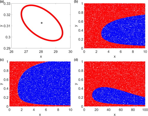
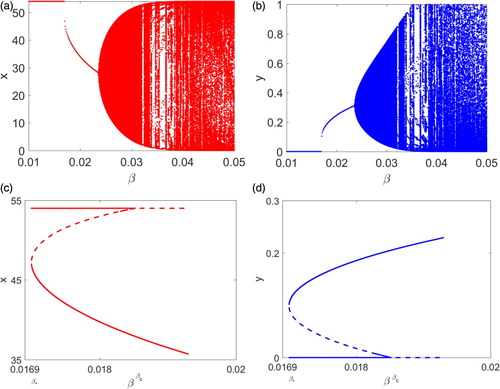
Figure 3. Bifurcation diagrams using β as the varying parameter are presented. (a)–(b) provide attractors of the system and a Neimark–Sacker bifurcation is shown. (c)–(d) plot steady states of the system when β lying in the narrow range $(0.0169962,0.018525)$ where solid and dashed lines denote stable and unstable steady states, respectively. A saddle-node bifurcation at $\beta ={\beta }_{\ast }$ is demonstrated.

Suppose now $\beta ={\beta }_c-0.0003$. Since ${\beta }_c-0.0003\approx 0.0185185>{\beta }_{\ast }\approx 0.0169961$, (3(3) $\begin{array}{rl}x(n+1)& =\frac{\lambda x\left(n\right)}{1+x\left(n\right)}{e}^{-y\left(n\right)(1+\alpha y(n\left)\right)}\\ y(n+1)& =\beta x\left(n\right)(1-e^{-y\left(n\right)(1+\alpha y(n\left)\right)}).\end{array}$(3) ) has two interior steady states $E_1^{\ast }\approx (53.46227,0.0095227)$ and $E_2^{\ast }\approx (38.928026,0.1943493)$, where $E_1^{\ast }$ is a saddle point and $E_2^{\ast }$ is asymptotically stable by Theorem 3.7 (c). We use 60,000 randomly generated initial conditions to determine basins of attraction for the steady states $E_1=(54,0)$ and $E_2^{\ast }$. Initial conditions that converge to $E_1$ and $E_2^{\ast }$ are denoted by red and blue colours, respectively. The simulation results are presented in Figure 2(b), where bistability of the system is illustrated. The region of initial conditions that converge to the stable interior steady state is smaller than the corresponding region for the stable boundary steady state.

We now decrease the α value to $\alpha =2$ with $\lambda =55$. Then ${\beta }_c\approx 0.0185485$, $y_c\approx 1.1874166$, $y_e\approx 0.10122834$, $y_d\approx 0.3816326>y_t=y_{\ast }\approx 0.0500192$. Using $\beta ={\beta }_c-0.00003\approx 0.0185185>{\beta }_{\ast }\approx 0.01829966$, there are two interior steady states $E_2^{\ast }\approx (47.94615,0.0975719)$ which is asymptotically stable and $E_1^{\ast }\approx (53.80683,0.003494)$ a saddle point. Randomly chosen 60000 initial conditions are used to explore the dynamics. Initial conditions that converge to $E_1=(54,0)$ and $E_2^{\ast }$ are denoted by red and blue colours, respectively, as shown in Figure 2(c). Although α for Figure 2(c) is smaller than the corresponding one for Figure 2(b), the β value is decreased only by 0.00003 and the region of converging to the stable interior steady state in Figure 2(c) is larger than the corresponding one in Figure 2(b).

Let $\lambda =95$ and $\alpha =25/3$. Then ${\beta }_c\approx 0.0106$, $2\alpha -\left(\right(3\lambda -1\left)/\right(\lambda -1\left)\right)a\approx 13.65>0$, $y_c\approx 0.6871$, $y_e\approx 0.24623>y_d\approx 0.213977$, $y_{\ast }\approx 0.112561$, $\overline{x}=94$ and ${\beta }_{\ast }\approx 0.0076189$. Let $\beta ={\beta }_c-0.005/3\approx 0.00893>{\beta }_{\ast }$. There are two interior steady states $E_1^{\ast }\approx (90.3822,0.03088)$, a saddle point, and $E_2^{\ast }\approx (53.6657,0.20442)$ which is asymptotically stable. This confirms Theorem 3.7(a) since $y_2^{\ast }<y_d<y_e$. Figure 2(d) provides basins of attraction for $E_1=(94,0)$ and $E_2^{\ast }$ with red and blue colors respectively. We observe that the red region in Figure 2(d) is connected just as the red regions in Figure 2(b),(c).

Finally, we present bifurcation diagrams using β as the varying parameter. Here $\lambda =55$ and $\alpha =10/3$, that is, parameter values of those in Figure 2(a ,b) are used. The first 1000 iterations are discarded and the next 1000 iterations are plotted in Figure 3(a ,b) so that only the attractors are shown. Notice that β lies in $[0.01,0.05]$ containing both ${\beta }_{\ast }\approx 0.0169961$ and ${\beta }_c\approx 0.01852$. It is clear that when β is in $(0.02,0.03)$ the system has a unique interior steady state and a Neimark–Sacker bifurcation occurs when the steady state becomes unstable. Since Figure 3(a),(b) provide only attractors, to illustrate the saddle-node bifurcation at $\beta ={\beta }_{\ast }$, we plot steady states when β is in $(0.0169962,0.018525)$ in Figure 3(c,d). The solid and dashed curves denote stable and unstable steady states, respectively. It is clear in these plots that the system has two interior steady states when $\beta \in ({\beta }_{\ast },{\beta }_c)$ and there is a unique interior steady state when $\beta >{\beta }_c$ and $\beta \approx {\beta }_c$.

5. Summary and discussion

This investigation is motivated by the recent work of Alves and Hilker [2] who use continuous-time models of predator–prey interactions with cooperative hunting in predators to study the impacts of cooperation upon population interactions. There are many populations with non-overlapping generations and discrete-time models are more appropriate to describe such populations. Further, ecological data collected are usually in discrete formats. Consequently, Chow et al. [4] derive a discrete-time predator–prey system with hunting cooperation within the predators. The discrete model is based on the classical Nichelson–Bailey system with density dependent host growth rate and cooperative hunting of the predator is modelled via the attack rate of the predator. An earlier research [6] proves that predators go extinct when there is no cooperative hunting and $\beta \overline{x}<1$, where $\beta \overline{x}$ may be interpreted as the predator's maximal reproductive number since it is the reproductive number of predators when the prey population is stabilized at its carrying capacity $\overline{x}=\lambda -1$. The study of [4] further concludes that the predators also go extinct if the maximal reproductive number is less than one and the degree of cooperative hunting is not large, i.e. $2\alpha \le \left(3\lambda -1\right)/\left(\lambda -1\right)$.

Under the condition that the maximal reproductive number of predators is less than one, the study carried out in [4] shows that the discrete model (3(3) $\begin{array}{rl}x(n+1)& =\frac{\lambda x\left(n\right)}{1+x\left(n\right)}{e}^{-y\left(n\right)(1+\alpha y(n\left)\right)}\\ y(n+1)& =\beta x\left(n\right)(1-e^{-y\left(n\right)(1+\alpha y(n\left)\right)}).\end{array}$(3) ) can have either zero, one or two interior steady states when the degree of cooperation is large, i.e. $2\alpha >\left(3\lambda -1\right)/\left(\lambda -1\right)$. The present investigation continues the study of the model by establishing local stability of the interior steady states analytically and by exploring asymptotic dynamics of the system when the parameters are within this regime.

We find out with intense cooperative hunting, Theorems 3.6 and 3.7 of the present study suggest that strong cooperative hunting in predators can promote predator persistence when its maximal reproductive number is less than one. Indeed, in this circumstance the interaction has two coexisting steady states if the predator's conversion β exceeds a critical value ${\beta }_{\ast }$, i.e. $\beta >{\beta }_{\ast }$. If predator's conversion is less than ${\beta }_{\ast }$, then cooperative hunting cannot prevent predator extinction. We prove analytically that the interior steady state that is close to the predator extinction steady state is always a saddle point while the other one can change stability from asymptotically stable to a repeller. Our numerical simulations indicate that the change of this stability is through a supercritical Neimark–Sacker bifurcation. As a consequence, both populations can coexist indefinitely if initial populations are in the basin of stable coexisting steady state or of an attracting invariant closed curve. It follows that cooperative hunting can mediate predator persistence.

To compare our results with those of Alves and Hilker [2], first noticing both studies conclude that cooperative hunting can promote predator persistence. While the conclusion in [2] is drawn from numerical investigations, our result is based on mathematical analysis. In particular, the degree of cooperative hunting in this study is quantified explicitly via $\alpha >\left(3\lambda -1\right)/2(\lambda -1)$. The inequality provides a relation between the degree α of predator cooperation and the growth rate λ of prey population. In addition, we prove that one of the coexisting steady states is always a saddle point, which was not shown analytically in [2]. However, since solutions of continuous-time models are continuous and unique for initial value problems, the stable manifold of the saddle interior steady state in [2] is a continuous decreasing curve separating the positive coordinate plane into two positively invariant regions with the region that lies below the stable manifold resulting in predator extinction. This stable manifold is termed as the predator's Allee threshold by Alves and Hilker [2]. The predator can survive as long as population distributions are above the threshold. This finding is no longer true for the discrete-time system as illustrated numerically in Figure 2. Specifically, the region for predator extinction includes not only those small predator populations but also large predator populations. Therefore, the predator Allee threshold in the discrete-time setting is more complicated than a strictly decreasing curve demonstrated numerically in [2].

This study concludes that cooperative hunting of predators may provide a mechanism for predator persistence when the environment is not favourable. Our result may have significant implications in biological control using predators since cooperative hunting can induce Allee effects in predators, which may cause biological control failure. Additionally, from the geometry of the basin of attraction of the predator extinction steady state, predators may go extinct even if the population sizes seem large at observation.

Acknowledgements

The authors thank both referees for their helpful comments and suggestions that improved the original manuscript. S. Jang thanks the Institute of Mathematics, Academia Sinica, Taiwan, for its financial and staff support for her summer and winter 2017 visits.

Disclosure statement

No potential conflict of interest was reported by the author(s).

Additional information

Funding

Y. Chow was partly supported by a grant from MOST, ROC. H.-M. Wang was supported by National Nature Science Foundation of China and Nature Science Foundation of Anhui Province (grant number 11501008; 1508085QA12).

References

- L.J.S. Allen, An Introduction to Mathematical Biology, Prentice-Hall, Upper Saddle River, NJ, 2006.
- M. Alves and F.M. Hilker, Hunting cooperation and Allee effects in predators, J. Theo. Biol. 419 (2017), pp. 13–22. doi: 10.1016/j.jtbi.2017.02.002
- L. Berec, Impacts of foraging facilitation among predators on predator-prey dynamics, Bull. Math. Biol. 72 (2010), pp. 94–121. doi: 10.1007/s11538-009-9439-1
- Y. Chow, S.R-J. Jang and H.M. Wang, Cooperative hunting in a discrete predator-prey system, submitted (2018), Available at https://arxiv.org/abs/1808.00182.
- C. Cosner, D.I. DeAngelis, J. Ault and D. Olson, Effects of spatial grouping on the functional response of predators, Theor. Popul. Biol. 56 (1999), pp. 65–75. doi: 10.1006/tpbi.1999.1414
- S.R-J. Jang, Allee effects in a discrete-time host-parasitoid model, J. Diff. Equ. Appl. 12 (2006), pp. 165–181. doi: 10.1080/10236190500539238
- R.M. May, Simple models with very complicated dynamics, Nature 261 (1976), pp. 459–467. doi: 10.1038/261459a0
- D. Scheel and C. Packer, Group hunting behavior of lions: a search for cooperation, Anim. Behav. 41 (1991), pp. 697–709. doi: 10.1016/S0003-3472(05)80907-8
- G.W. Uetz, Foraging strategies of spiders, Trends Ecol. Evol. 7 (1992), pp. 155–159. doi: 10.1016/0169-5347(92)90209-T