A discrete host-parasitoid model with development of pesticide resistance and IPM strategies

ABSTRACT

The development of pesticide resistance significantly affects the outcomes of pest control. A quantitative depiction of the effects of pesticide resistance development on integrated pest management (IPM) strategies and pest control outcomes is challenging. To address this problem, a discrete host-parasitoid model with pesticide resistance development and IPM strategies is proposed and analyzed. The threshold condition of pest eradication which reveals the relationship between the development of pest resistance and the rate of natural enemy releases is provided and analyzed, and the optimal rate for releasing natural enemies was obtained based on this threshold condition. Furthermore, in order to reduce adverse effects of the pesticide on natural enemies, the model has been extended to consider the spraying of pesticide and releases of natural enemies at different times. The effects of the dynamic complexity and different resistance development equations on the main results are also discussed.

KEYWORDS:

• IPM
• resistance
• host-parasitoid model
• biological control
• dynamic threshold

1. Introduction

Integrated pest management (IPM) involves choosing appropriate tactics from a range of pest control techniques including biological, cultural and chemical methods to maintain the density of the pest population below the Economic Injury Level (EIL) [8, 41–43]. It is well known that single chemical control tactics are usually inefficient, because they may result in high rates of failure due to rapid evolution of pest resistance. If so, a combination of biological and chemical control tactics is often necessary for successful pest control. Thus, biological control, defined as the reduction of pest populations by natural enemies, is often a key component of an IPM strategy [10, 31] and typically requires impulsive perturbations such as augmentation of natural enemies. Augmentation involves the supplemental release of natural enemies at critical times of the season when insufficient reproduction of released natural enemies is likely to occur, allowing pest control to be achieved exclusively by the released individuals [13, 27].

Forecasting trends in density changes of a pest population is a key factor in pest control, which requires mathematical models. Hybrid models with both continuous and discrete equations (such as impulsive differential equations) have been widely used in IPM [16, 24, 27, 31, 34, 36–39]. In most of these studies, trends in pest population density changes were modelled with continuous mathematical models. In reality, many pests' individual growth is not continuous, especially when pest generations do not overlap, so discrete models are more appropriate for modelling trends in such pest population densities. Note that a discrete model with an IPM strategy was first proposed by Tang et al. [35], in which a classical host-parasitoid model was employed and analyzed. In particular, both chemical control and biological control were applied at certain generations with proportional reductions in the density of the pest population and a constant release rate of natural enemies. The effects of IPM on the dynamics of a discrete model and on pest control were studied.

Chemical control is one of the main tactics in IPM. However, with long term and high frequency use of chemical pesticides, pests have developed strong resistance to some pesticides. Studies have shown that more than 500 species of pests have now developed resistance to certain pesticides [9, 11, 15, 40], leading to outbreaks or resurgence of pests and increased crop losses. Farmers in the USA lost 7% of their crops to pests in the 1940s, while since the 1980s, the percentage lost has increased to 13%, even though more pesticides were being used [11, 14, 32]. Therefore, how to fight the development of pest resistance is an important problem in pest control. Some principles are suggested to defeat the evolution of pest resistance including pesticide rotation or switching, avoiding unnecessary pesticide applications, using non-chemical control techniques [7, 19, 21], and leaving untreated refuges where susceptible pests can survive [22].

Combining population dynamics with genetics, May and Dobson modelled the evolution of pest resistance [25]. Considering the effects of the frequency and the dosages of pesticide applications on the evolution of pesticide resistance, the simplest single species model with evolution of pesticide resistance has been proposed and analyzed by Liang et al. [21], who used different threshold levels for three different switching strategies to counter the evolution of pest resistance. Moreover, optimal switching times and optimal switching strategies were discussed in detail, and some important issues related to pest control and resistance management methods were addressed [21]. Unfortunately, the effects of biological control on those optimal strategies, which could significantly affect the evolution of pesticide resistance and pest control [8, 18, 20, 29, 41–43], were not investigated in that study. As mentioned above, biological control together with chemical control should be more effective when using IPM strategies. The combined use of Abamectin and Encarsia formosa Gahan (Hymenoptera: Aphelinidae) against the greenhouse whitefly, Trialeurodes vaporariorum Westwood (Homoptera: Aleyrodidae) [44] is one such example, and other cases can be found in the literature [23, 28].

Given that discrete host-parasitoid models can depict the dynamics of both pest and natural enemy populations, they can be useful for designing optimal strategies to fight against the evolution of pesticide resistance. The main purpose of this paper is to reveal the relationship between the development of pest resistance and the number of natural enemies to be released. Questions to be addressed include how to model the development of pest resistance in discrete natural enemy-pest systems? What is the relationship between the development of pest resistance and releasing strategies? And how many natural enemies should be released as pest resistance develops? To address these questions, the threshold conditions which guarantee the stability of pest free periodic solutions have been obtained, which involve the density of natural enemies and the effects of dosage, frequency, and times of pesticide spraying.

2. Discrete models for pest population growth and the development of pesticide resistance

As mentioned in the introduction, non-overlapping generations of most pest populations should be modelled with discrete or difference equations. Moreover, the frequent spraying of pesticides will cause the evolution of pesticide resistance to appear quickly, which in turn results in pest outbreaks or resurgence. Factors including the growth of the pest population, the frequency of the pesticide sprays and the evolution of pesticide resistance together could significantly affect the success of pest control. Therefore, in order to show these in more detail, we first propose simple discrete models for pest population growth and development of pesticide resistance in this section.

Discrete single species models including the Beverton-Holt model and the Ricker model have been widely used for describing pest population growth, and in the present work we assume that the pest population follows the Beverton-Holt model in the absence of natural enemies, i.e. we have (1) $P_{t+1}=\frac{a{P}_t}{1+b{P}_t},$(1) where $P_t$ denotes the density of the pest population at generation t, a represents the intrinsic growth rate and K (here $b=(a-1)/K$) denotes the carrying capacity of the pest population. Note that because the model does not allow for different gene frequencies resulting from sexual reproduction other than wholly resistant or completely susceptible insects, the model can only be used to describe populations with genetically fixed resistant or susceptible populations or to insects which undergo parthenogenetic reproduction.

To develop a model for describing the development of pesticide resistance, we divide the pest population into two parts: susceptible pests (denoted by $P_t^s$), which accounts for ${\omega }_t$ of the pest population at generation t and resistant pests (denoted by $P_t^r$), which accounts for $1-{\omega }_t$ of the pest population at generation t. Thus, the evolution of pest resistance can be depicted by ${\omega }_t$ with the development of generation t. Throughout this study, we assume that the pesticides are sprayed periodically with period q-generations ($q\ge 1$). Without loss of generality, we assume that pesticides are sprayed at time $t=q,2q,3q,\dots$, and the death rates due to pesticide applications of the susceptible pests and the resistant pests are $d_1(0<d_1<1)$ and $d_2$ (in this paper, we assume that $d_2=0$), respectively. According to model (1(1) $P_{t+1}=\frac{a{P}_t}{1+b{P}_t},$(1) ), we have $\begin{array}{rl}{P}_{kq}^s& =\frac{(1-d_1)a{\omega }_{kq-1}{P}_{kq-1}}{1+b{P}_{kq-1}},\\ P_{kq}^r& =\frac{a(1-{\omega }_{kq-1})P_{kq-1}}{1+b{P}_{kq-1}},\end{array}$ where $k=1,2,\dots$. Thus, $P_{kq}=P_{kq}^s+P_{kq}^r=\frac{(1-d_1)a{\omega }_{kq-1}{P}_{kq-1}+a(1-{\omega }_{kq-1})P_{kq-1}}{1+b{P}_{kq-1}}.$ Due to ${\omega }_t=P_t^s/P_t$, we have ${\omega }_{kq}=\frac{(1-d_1){\omega }_{kq-1}}{1-d_1{\omega }_{kq-1}}.$ Note that the pesticide is not sprayed at time $t=(k-1)q+1,(k-1)q+2,\dots ,kq-1$, which indicates that ${\omega }_{(k-1)q}={\omega }_{(k-1)q+1}=\cdots ={\omega }_{kq-1}$. Thus, we have the resistant population equations as follows: (2) $\begin{array}{rl}{\omega }_{kq}& =\frac{(1-d_1){\omega }_{(k-1)q}}{1-d_1{\omega }_{(k-1)q}},\\ {\omega }_{(k-1)q}& ={\omega }_{(k-1)q+1}=\cdots ={\omega }_{kq-1}.\end{array}$(2) Solving this equation yields (3) ${\omega }_{kq}=\frac{(1-d_1{)}^k{\omega }_0}{1-d_1{\omega }_0\sum _{i=0}^{k-1}(1-d_1{)}^i},k>0.$(3) The effects of the development of pesticide resistance on the pest control described by single species model (1(1) $P_{t+1}=\frac{a{P}_t}{1+b{P}_t},$(1) ) and Equation (2(2) $\begin{array}{rl}{\omega }_{kq}& =\frac{(1-d_1){\omega }_{(k-1)q}}{1-d_1{\omega }_{(k-1)q}},\\ {\omega }_{(k-1)q}& ={\omega }_{(k-1)q+1}=\cdots ={\omega }_{kq-1}.\end{array}$(2) ) for pesticide resistance have been extensively investigated by Liang et al. [21]. The question is how do natural enemy releasing strategies affect the pest control under the development of pesticide resistance, which will be studied in the following.

3. Discrete host-parasitoid model with development of pesticide resistance

A discrete model with an IPM strategy was first proposed by Tang et al. [35], in which a classical host-parasitoid model was employed and analyzed. In particular, both chemical control and biological control were applied at certain generations with a proportional reduction of the density of the host population and a constant releasing rate of natural enemies. The effects of IPM on the dynamics of this discrete model and on pest control were studied. However, as mentioned in the introduction, the effects of the development of pesticide resistance on the releasing strategies of natural enemies should also be involved in such a discrete model and carefully investigated.

Therefore, considering the effects of natural enemies on the pests and assuming that natural enemy releases and the spraying of pesticides occur impulsively, we can extend model (1(1) $P_{t+1}=\frac{a{P}_t}{1+b{P}_t},$(1) ) as follows: (4) $\begin{array}{r}\left\{\begin{array}{c}\left.\begin{array}{l}{P}_{t+1}=\frac{a{P}_t}{1+b{P}_t}{e}^{-\alpha N_t},\\ N_{t+1}=\beta P_t\left(1-e^{-\alpha N_t}\right)+d{N}_t,\end{array}\right\}t=1,2,\dots ,\\ \left.\begin{array}{l}{\omega }_{qk}=\frac{(1-d_1){\omega }_{q(k-1)}}{1-d_1{\omega }_{q(k-1)}},\\ P_{q{k}^{+}}=(1-d_1{\omega }_{qk})P_{qk},\\ N_{q{k}^{+}}=N_{qk}+{\delta }_k,\end{array}\right\}k=1,2,\dots ,\end{array}\right.\end{array}$(4) with initial value $P_0^{+}=P_0,N_0^{+}={\delta }_0,{\omega }_0,$ where $r_k=k/q,$ and $N_t$ is the population size of the natural enemy at time t, α is a measure of the natural enemies' searching efficiency, and the term $\exp (-\alpha N_t)$ is the probability that a pest individual escapes being eaten, if the natural enemy is a predator, or parasitized if the natural enemy is a parasitoid, β is the conversion rate of a pest individual into a natural enemy, d is the survival rate of the natural enemy from time t to time t+1 and at each impulsive time kq, ${\delta }_k$ natural enemies are released and pesticide is sprayed, $n\in \mathcal{N}$, $d_1$ is the mortality rate of susceptible pests after each chemical control. Since the third equation of system (4(4) $\begin{array}{r}\left\{\begin{array}{c}\left.\begin{array}{l}{P}_{t+1}=\frac{a{P}_t}{1+b{P}_t}{e}^{-\alpha N_t},\\ N_{t+1}=\beta P_t\left(1-e^{-\alpha N_t}\right)+d{N}_t,\end{array}\right\}t=1,2,\dots ,\\ \left.\begin{array}{l}{\omega }_{qk}=\frac{(1-d_1){\omega }_{q(k-1)}}{1-d_1{\omega }_{q(k-1)}},\\ P_{q{k}^{+}}=(1-d_1{\omega }_{qk})P_{qk},\\ N_{q{k}^{+}}=N_{qk}+{\delta }_k,\end{array}\right\}k=1,2,\dots ,\end{array}\right.\end{array}$(4) ) is independent of the former two equations, according to (3(3) ${\omega }_{kq}=\frac{(1-d_1{)}^k{\omega }_0}{1-d_1{\omega }_0\sum _{i=0}^{k-1}(1-d_1{)}^i},k>0.$(3) ) we can solve ${\omega }_{kq}$.

Note that in system (4(4) $\begin{array}{r}\left\{\begin{array}{c}\left.\begin{array}{l}{P}_{t+1}=\frac{a{P}_t}{1+b{P}_t}{e}^{-\alpha N_t},\\ N_{t+1}=\beta P_t\left(1-e^{-\alpha N_t}\right)+d{N}_t,\end{array}\right\}t=1,2,\dots ,\\ \left.\begin{array}{l}{\omega }_{qk}=\frac{(1-d_1){\omega }_{q(k-1)}}{1-d_1{\omega }_{q(k-1)}},\\ P_{q{k}^{+}}=(1-d_1{\omega }_{qk})P_{qk},\\ N_{q{k}^{+}}=N_{qk}+{\delta }_k,\end{array}\right\}k=1,2,\dots ,\end{array}\right.\end{array}$(4) ), we assume that in absence of pesticides, the resistant strains are as fit as the sensitive ones; Pesticides decay quickly, so that negative effects occur only in the same generation of spraying, and natural enemies are not affected by pesticides.

What we want to address for model (4(4) $\begin{array}{r}\left\{\begin{array}{c}\left.\begin{array}{l}{P}_{t+1}=\frac{a{P}_t}{1+b{P}_t}{e}^{-\alpha N_t},\\ N_{t+1}=\beta P_t\left(1-e^{-\alpha N_t}\right)+d{N}_t,\end{array}\right\}t=1,2,\dots ,\\ \left.\begin{array}{l}{\omega }_{qk}=\frac{(1-d_1){\omega }_{q(k-1)}}{1-d_1{\omega }_{q(k-1)}},\\ P_{q{k}^{+}}=(1-d_1{\omega }_{qk})P_{qk},\\ N_{q{k}^{+}}=N_{qk}+{\delta }_k,\end{array}\right\}k=1,2,\dots ,\end{array}\right.\end{array}$(4) ) is to investigate how to design the releasing constant ${\delta }_k$ as pesticide resistance develops. Of particular interest is to determine the value ${\delta }_k$ for the fixed period q such that the pest population dies out eventually without switching pesticides.

3.1. Threshold condition for the pest-free solution

The basic properties of the following subsystem (5) $\begin{array}{rl}& N_{t+1}=d{N}_t,t=1,2,\dots ,\\ & N_{q{k}^{+}}=N_{qk}+{\delta }_k,k=1,2,\dots ,\\ & N_0={\delta }_0,\end{array}$(5) play key roles for the investigation of model (4(4) $\begin{array}{r}\left\{\begin{array}{c}\left.\begin{array}{l}{P}_{t+1}=\frac{a{P}_t}{1+b{P}_t}{e}^{-\alpha N_t},\\ N_{t+1}=\beta P_t\left(1-e^{-\alpha N_t}\right)+d{N}_t,\end{array}\right\}t=1,2,\dots ,\\ \left.\begin{array}{l}{\omega }_{qk}=\frac{(1-d_1){\omega }_{q(k-1)}}{1-d_1{\omega }_{q(k-1)}},\\ P_{q{k}^{+}}=(1-d_1{\omega }_{qk})P_{qk},\\ N_{q{k}^{+}}=N_{qk}+{\delta }_k,\end{array}\right\}k=1,2,\dots ,\end{array}\right.\end{array}$(4) ).

The analytical solution of this subsystem at any impulsive interval $(kq,(k+1\left)q\right]$ gives (6) $N^{\ast }\left(t\right)=d^t\sum _{i=0}^k{\delta }_i{d}^{-iq},kq<t\le (k+1)q.$(6) Therefore, the expression for the pest-free solution of system (4(4) $\begin{array}{r}\left\{\begin{array}{c}\left.\begin{array}{l}{P}_{t+1}=\frac{a{P}_t}{1+b{P}_t}{e}^{-\alpha N_t},\\ N_{t+1}=\beta P_t\left(1-e^{-\alpha N_t}\right)+d{N}_t,\end{array}\right\}t=1,2,\dots ,\\ \left.\begin{array}{l}{\omega }_{qk}=\frac{(1-d_1){\omega }_{q(k-1)}}{1-d_1{\omega }_{q(k-1)}},\\ P_{q{k}^{+}}=(1-d_1{\omega }_{qk})P_{qk},\\ N_{q{k}^{+}}=N_{qk}+{\delta }_k,\end{array}\right\}k=1,2,\dots ,\end{array}\right.\end{array}$(4) ) over the nth time interval $kq<t\le (k+1)q$ is given by (7) $(0,N_t^{\ast })=\left(0,d^t\sum _{i=0}^k{\delta }_i{d}^{-iq}\right).$(7) For $k\in \mathcal{N}$, we denote $R_1(k,q)=\left(1-d_1{\omega }_{kq}\right)a^q,R_2(k,q)=\exp \left(-\alpha \left(\sum _{i=0}^k{\delta }_i{d}^{(k-i)q}\right)\left(\sum _{i=0}^q{d}^i\right)\right)$ and (8) $R_0(k,q)=R_1(k,q)R_2(k,q).$(8) Then we have the following threshold theorem for the pest-free solution.

Theorem 3.1

Let $(P_t,N_t)$ be any solution of system (4(4) $\begin{array}{r}\left\{\begin{array}{c}\left.\begin{array}{l}{P}_{t+1}=\frac{a{P}_t}{1+b{P}_t}{e}^{-\alpha N_t},\\ N_{t+1}=\beta P_t\left(1-e^{-\alpha N_t}\right)+d{N}_t,\end{array}\right\}t=1,2,\dots ,\\ \left.\begin{array}{l}{\omega }_{qk}=\frac{(1-d_1){\omega }_{q(k-1)}}{1-d_1{\omega }_{q(k-1)}},\\ P_{q{k}^{+}}=(1-d_1{\omega }_{qk})P_{qk},\\ N_{q{k}^{+}}=N_{qk}+{\delta }_k,\end{array}\right\}k=1,2,\dots ,\end{array}\right.\end{array}$(4) ). Then the pest-free solution (7(7) $(0,N_t^{\ast })=\left(0,d^t\sum _{i=0}^k{\delta }_i{d}^{-iq}\right).$(7) ) is globally attractive if $R_0(k,q)\le 1$ for all $k\in \mathcal{N}$.

Proof.

It is seen from the second equation of system (4(4) $\begin{array}{r}\left\{\begin{array}{c}\left.\begin{array}{l}{P}_{t+1}=\frac{a{P}_t}{1+b{P}_t}{e}^{-\alpha N_t},\\ N_{t+1}=\beta P_t\left(1-e^{-\alpha N_t}\right)+d{N}_t,\end{array}\right\}t=1,2,\dots ,\\ \left.\begin{array}{l}{\omega }_{qk}=\frac{(1-d_1){\omega }_{q(k-1)}}{1-d_1{\omega }_{q(k-1)}},\\ P_{q{k}^{+}}=(1-d_1{\omega }_{qk})P_{qk},\\ N_{q{k}^{+}}=N_{qk}+{\delta }_k,\end{array}\right\}k=1,2,\dots ,\end{array}\right.\end{array}$(4) ) that $N_{t+1}\ge d{N}_t$. Consider the following impulsive difference equation (9) $\begin{array}{rl}& y_{t+1}=d{y}_t,t=1,2,\dots ,\\ & y_{q{k}^{+}}=y_{qk}+{\delta }_k,k=1,2,\dots ,\\ & y_0={\delta }_0.\end{array}$(9) According to the comparison theorem on impulsive difference equations, we have $N_t\ge y_t=N_t^{\ast }$. Therefore, according to the first equation of system (4(4) $\begin{array}{r}\left\{\begin{array}{c}\left.\begin{array}{l}{P}_{t+1}=\frac{a{P}_t}{1+b{P}_t}{e}^{-\alpha N_t},\\ N_{t+1}=\beta P_t\left(1-e^{-\alpha N_t}\right)+d{N}_t,\end{array}\right\}t=1,2,\dots ,\\ \left.\begin{array}{l}{\omega }_{qk}=\frac{(1-d_1){\omega }_{q(k-1)}}{1-d_1{\omega }_{q(k-1)}},\\ P_{q{k}^{+}}=(1-d_1{\omega }_{qk})P_{qk},\\ N_{q{k}^{+}}=N_{qk}+{\delta }_k,\end{array}\right\}k=1,2,\dots ,\end{array}\right.\end{array}$(4) ), we can get $P_{t+1}\le \frac{a{P}_t}{1+b{P}_t}{e}^{-\alpha N_t^{\ast }}.$ Now we consider the following impulsive differential equation (10) $\begin{array}{r}\left\{\begin{array}{c}{\overline{P}}_{t+1}=\frac{a{\overline{P}}_t}{1+b{\overline{P}}_t}{e}^{-\alpha N_t^{\ast }},t=1,2,\dots ,\\ \left.\begin{array}{l}{\omega }_{qk}=\frac{(1-d_1){\omega }_{(k-1)q}}{1-d_1{\omega }_{(k-1)q}},\\ {\overline{P}}_{q{k}^{+}}=(1-d_1{\omega }_{qk}){\overline{P}}_{qk},\end{array}\right\}k=1,2,\dots .\end{array}\right.\end{array}$(10) Again, according to the comparison theorem on impulsive difference equations we have $P_t\le {\overline{P}}_t$.

Solving system (10(10) $\begin{array}{r}\left\{\begin{array}{c}{\overline{P}}_{t+1}=\frac{a{\overline{P}}_t}{1+b{\overline{P}}_t}{e}^{-\alpha N_t^{\ast }},t=1,2,\dots ,\\ \left.\begin{array}{l}{\omega }_{qk}=\frac{(1-d_1){\omega }_{(k-1)q}}{1-d_1{\omega }_{(k-1)q}},\\ {\overline{P}}_{q{k}^{+}}=(1-d_1{\omega }_{qk}){\overline{P}}_{qk},\end{array}\right\}k=1,2,\dots .\end{array}\right.\end{array}$(10) ),we have (11) ${\overline{P}}_{(k+1)q}=\frac{a^q{e}^{-\alpha \left(\sum _{i=0}^k{\delta }_i{d}^{(k-i)q}\right)\left(\sum _{i=0}^{q-1}{d}^i\right)}(1-d_1{\omega }_{kq}){\overline{P}}_{kq}}{1+b\left(1+\sum _{j=1}^{q-2}{a}^j{e}^{-\alpha \left(\sum _{i=0}^k{\delta }_i{d}^{(k-i)q}\right)\left(\sum _{i=0}^j{d}^i\right)}\right)(1-d_1{\omega }_{kq}){\overline{P}}_{kq}},$(11) where ${\omega }_{kq}$ is given by (3(3) ${\omega }_{kq}=\frac{(1-d_1{)}^k{\omega }_0}{1-d_1{\omega }_0\sum _{i=0}^{k-1}(1-d_1{)}^i},k>0.$(3) ).

Letting $Y_k={\overline{P}}_{kq}$, we have $Y_{k+1}=\frac{a^q{e}^{-\alpha \left(\sum _{i=0}^k{\delta }_i{d}^{(k-i)q}\right)\left(\sum _{i=0}^{q-1}{d}^i\right)}(1-d_1{\omega }_{kq})Y_k}{1+b\left(1+\sum _{j=1}^{q-2}{a}^j{e}^{-\alpha \left(\sum _{i=0}^k{\delta }_i{d}^{(k-i)q}\right)\left(\sum _{i=0}^j{d}^i\right)}\right)(1-d_1{\omega }_{kq})Y_k},$ note that this is the classical Beverton-Holt model, and if $R_0(k,q)\le 1$, then $Y_k\to 0$ as $k\to 0$. This indicates that ${\overline{P}}_{kq}\to 0$ as $k\to 0$. Due to ${\overline{P}}_t<{\overline{P}}_{kq}$, for $(k-1)q<t\le kq$, therefore, ${\overline{P}}_t\to 0$ as $t\to \mathrm{\infty }$. Because $0<P_t\le {\overline{P}}_t$, then, $P_t\to 0$ as $t\to \mathrm{\infty }$.

Next, we prove that $N_t\to N_t^{\ast }$ as $t\to \mathrm{\infty }$. For any $\epsilon >0$, there exists a $t_1>0$ such that $0<P_t<\epsilon$ for all $t\ge t_1$. Without loss of generality, we may assume that $0<P_t<\epsilon$ holds true for all t>0, then we have $d{N}_t\le N_{t+1}\le \beta \epsilon +d{N}_t.$ For the left hand inequality, it follows from impulsive difference equation (9(9) $\begin{array}{rl}& y_{t+1}=d{y}_t,t=1,2,\dots ,\\ & y_{q{k}^{+}}=y_{qk}+{\delta }_k,k=1,2,\dots ,\\ & y_0={\delta }_0.\end{array}$(9) ) that $N_t\ge y_t=N_t^{\ast }$. For the right hand inequality, considering the following impulsive difference equation (12) $\begin{array}{rl}& X_{t+1}=\beta \epsilon +d{X}_t,t=1,2,\dots ,\\ & X_{k{q}^{+}}=X_{kq}+{\delta }_k,k=1,2,\dots ,\\ & X_{0^{+}}=N_0={\delta }_0.\end{array}$(12) The analytical solution of the above system at any impulsive interval $(kq,(k+1\left)q\right]$ gives (13) $X_t^{\ast }=\beta \epsilon \left(\sum _{i=0}^{t-1}{d}^i\right)+\sum _{i=0}^k{\delta }_i{d}^{t-iq}=\beta \epsilon \left(\sum _{i=0}^{t-1}{d}^i\right)+N_t^{\ast },kq<t\le (k+1)q.$(13) According to the comparison theorem on impulsive difference equations, we have $N_t\le X_t^{\ast }$. Therefore, for any ${\epsilon }_1>0$, there exists a $t_2>0$ such that $N_t^{\ast }-{\epsilon }_1<N_t<X_t^{\ast }+{\epsilon }_1$ for $t>t_2$. Let $\epsilon \to 0$, then we have $N_t^{\ast }-{\epsilon }_1<N_t<N_t^{\ast }+{\epsilon }_1$ for $t>t_2$, which indicates that $N_t\to N_t^{\ast }$ as $t\to \mathrm{\infty }$. Therefore, the pest-free solution (7(7) $(0,N_t^{\ast })=\left(0,d^t\sum _{i=0}^k{\delta }_i{d}^{-iq}\right).$(7) ) is globally attractive if $R_0^N(k,q)\le 1$.

It is interesting to note that the expression of $R_0(k,q)$ clearly shows the effects of IPM strategies on the pest control: if only the chemical control is applied, the threshold value $R_0(k,q)$ is reduced to $R_1(k,q)$ which is obviously larger than $R_0(k,q)$, due to $R_2(k,q)<1$. If only the biological control is implemented, the threshold value $R_0(k,q)$ is reduced to $a^q{R}_2(k,q)$, which is also lager than $R_0(k,q)$. Therefore, the threshold condition $R_0(k,q)$ confirms that an integrated control strategy is more effective than any single control strategy.

In particular, if ${\delta }_i=\delta$ for $i\in {\mathcal{N}}_0$, where ${\mathcal{N}}_0=\{0,1,2,3,\dots \}$, then for subsystem (5(5) $\begin{array}{rl}& N_{t+1}=d{N}_t,t=1,2,\dots ,\\ & N_{q{k}^{+}}=N_{qk}+{\delta }_k,k=1,2,\dots ,\\ & N_0={\delta }_0,\end{array}$(5) ) there exists a unique periodic solution, denoted by $N_t^T$ and $N_t^T=\delta d^t\sum _{i=0}^k{d}^{-iq},t\in (kq,(k+1\left)q\right],k\in \mathcal{N}$ with initial value $N_0^{+}=\delta$. It is easy to prove that for every solution $N_t$ of (5(5) $\begin{array}{rl}& N_{t+1}=d{N}_t,t=1,2,\dots ,\\ & N_{q{k}^{+}}=N_{qk}+{\delta }_k,k=1,2,\dots ,\\ & N_0={\delta }_0,\end{array}$(5) ) in the case of ${\delta }_i=\delta$ for $i\in {\mathcal{N}}_0$ we have $|N_t-N_t^T|\to 0$ as $t\to \mathrm{\infty }$. For this special case, the threshold value $R_0(k,q)$ turns into the following form: (14) $R_0(k,q)=R_1(k,q)\exp \left(-\frac{\alpha \delta \left(1-d^{(k+1)q}\right)}{1-d}\right)\doteq {\overline{R}}_0(k,q).$(14) Then the pest-free periodic solution $(0,N_t^T)$ is globally attractive provided that ${\overline{R}}_0(k,q)\le 1$.

3.2. Determining the new number of natural enemies to be released

The threshold value $R_0(k,q)$ reveals how the chemical and biological control tactics contribute to the pest control, in which $R_1(k,q)$ shows the effects of the frequency of pesticide applications and development of pest resistance on the control output, and the second part $R_2(k,q)$ represents the contribution of natural enemies. We know that $R_1(k,q)$ is a monotonically increasing function with respect to k and q, which indicates that chemical control alone will quickly fail once strong pesticide resistance develops. So the question is how to release the natural enemies such that the threshold value $R_0(k,q)$ or ${\overline{R}}_0(k,q)$ is relatively small, for example less than one forever? That is, how to determine ${\delta }_k$ or δ in $R_0(k,q)$ or ${\overline{R}}_0(k,q)$ such that those threshold values equal a constant $R_C$? Due to the complexity of $R_0(k,q)$, we first consider ${\overline{R}}_0(k,q)$.

In fact, solving equation (15) $R_1(k,q)\exp \left(-\frac{\alpha \delta \left(1-d^{(k+1)q}\right)}{1-d}\right)=R_C$(15) with respect to δ, yields (16) $\delta =-\frac{1-d}{\alpha \left(1-d^{(k+1)q}\right)}\ln \left(\frac{R_C}{R_1(k,q)}\right),k\in \mathcal{N}.$(16) If our aim is to eradicate the pest population, then the constant $R_C$ should be assumed to be less than one. There is an interesting fact from (16(16) $\delta =-\frac{1-d}{\alpha \left(1-d^{(k+1)q}\right)}\ln \left(\frac{R_C}{R_1(k,q)}\right),k\in \mathcal{N}.$(16) ) that if $R_1(k,q)\le R_C$ for some $k\in \mathcal{N}$, then $\delta \le 0$, which means that the chemical control alone can suppress the pest outbreak at the initial stage. However, once the pest resistance develops such that $R_1(k,q)>R_C$, then pulsed releases of natural enemies are necessary to maintain ${\overline{R}}_0(k,q)$ as a constant $R_C$. All these results confirm that the number of natural enemies to be released δ depends strictly on the number of pesticide applications k. Therefore, the number of natural enemies to be released δ for all $k\in \mathcal{N}$ can be defined as follows: (17) $\delta ={\delta }_k=\left\{\begin{array}{ll}{\delta }_c,& \text{if}{R}_1(k,q)\le R_C,\\ -\frac{1-d}{\alpha \left(1-d^{(k+1)q}\right)}\ln \left(\frac{R_C}{R_1(k,q)}\right),& \text{if}{R}_1(k,q)>R_C,\end{array}\right.$(17) where ${\delta }_c$ can be zero or a relatively small positive constant.

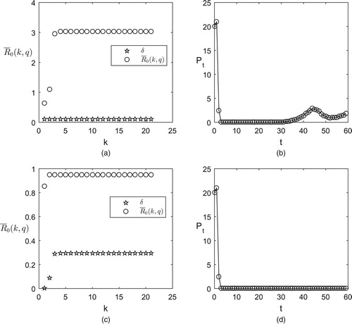
In order to clarify the way to release natural enemies according to the formula (17(17) $\delta ={\delta }_k=\left\{\begin{array}{ll}{\delta }_c,& \text{if}{R}_1(k,q)\le R_C,\\ -\frac{1-d}{\alpha \left(1-d^{(k+1)q}\right)}\ln \left(\frac{R_C}{R_1(k,q)}\right),& \text{if}{R}_1(k,q)>R_C,\end{array}\right.$(17) ) and constant number, we adopted numerical analyzes, see Figure 1. In Figure 1 (a) and (c), we plot the growing trend of the threshold values ${\overline{R}}_0(k,q)$ with the times of pesticide spraying k by using a strategy of releasing a constant number of natural enemies in which the number of natural enemies to be released δ is determined by formula (17(17) $\delta ={\delta }_k=\left\{\begin{array}{ll}{\delta }_c,& \text{if}{R}_1(k,q)\le R_C,\\ -\frac{1-d}{\alpha \left(1-d^{(k+1)q}\right)}\ln \left(\frac{R_C}{R_1(k,q)}\right),& \text{if}{R}_1(k,q)>R_C,\end{array}\right.$(17) ). From Figure 1 (a), we can see that the threshold value ${\overline{R}}_0(k,q)$ is increasing with respect to the times of pesticide spraying k, and exceeds 1 after spraying pesticide twice because of the development of pesticide resistance following farmers? releases of the same numbers of natural enemies every control time. And under this strategy, we can see that the density of the pest population is decreased at first because of the high efficiency of the pesticide. However, with the development of the pesticide resistance, the efficiency of pesticide drops and the pest population becomes resurgent (see Figure 1(b)), which means that pest control cannot be successful with a strategy of constant releases of low numbers of natural enemies. However, if we release natural enemies only when $R_1(k,q)>R_C$ and maintain ${\overline{R}}_0(k,q)=R_c$, that is ${\delta }_k$ is determined by formula (17(17) $\delta ={\delta }_k=\left\{\begin{array}{ll}{\delta }_c,& \text{if}{R}_1(k,q)\le R_C,\\ -\frac{1-d}{\alpha \left(1-d^{(k+1)q}\right)}\ln \left(\frac{R_C}{R_1(k,q)}\right),& \text{if}{R}_1(k,q)>R_C,\end{array}\right.$(17) ) and ${\delta }_c=0$ (see Figure 1(c)), the pest population will be eradicated after a certain number of times that pest control is conducted (see Figure 1(d)).

Figure 1. The threshold values ${\overline{R}}_0(k,q)$ and numerical simulations of model (4(4) $\begin{array}{r}\left\{\begin{array}{c}\left.\begin{array}{l}{P}_{t+1}=\frac{a{P}_t}{1+b{P}_t}{e}^{-\alpha N_t},\\ N_{t+1}=\beta P_t\left(1-e^{-\alpha N_t}\right)+d{N}_t,\end{array}\right\}t=1,2,\dots ,\\ \left.\begin{array}{l}{\omega }_{qk}=\frac{(1-d_1){\omega }_{q(k-1)}}{1-d_1{\omega }_{q(k-1)}},\\ P_{q{k}^{+}}=(1-d_1{\omega }_{qk})P_{qk},\\ N_{q{k}^{+}}=N_{qk}+{\delta }_k,\end{array}\right\}k=1,2,\dots ,\end{array}\right.\end{array}$(4) ) with constant pulse releasing of natural enemies. The baseline parameter values are as follows: ${\omega }_0=0.99,R_C=0.95,d_1=0.8,q=3,a=1.6,b=0.001,\alpha =2,\beta =0.1,d=0.6$ and ${\delta }_c=0$ (a) The plot of ${\overline{R}}_0(k,q)$ with respect to k and $\delta =0.2$; (b) The time series of the pest population associated with (a); (c) The plot of ${\overline{R}}_0(k,q)$ with respect to k and the releasing constant δ determined by formula (17(17) $\delta ={\delta }_k=\left\{\begin{array}{ll}{\delta }_c,& \text{if}{R}_1(k,q)\le R_C,\\ -\frac{1-d}{\alpha \left(1-d^{(k+1)q}\right)}\ln \left(\frac{R_C}{R_1(k,q)}\right),& \text{if}{R}_1(k,q)>R_C,\end{array}\right.$(17) ); (d) The time series of the pest population associated with (c).

Now let us turn to the general case, i.e. the threshold value $R_0(k,q)$.

In this case, we let $R_0(k,q)=R_c$. It follows from (8(8) $R_0(k,q)=R_1(k,q)R_2(k,q).$(8) ) that we have $R_1(k,q)e^{-\alpha \left(\sum _{i=0}^k{\delta }_i{d}^{(k-i)q}\right)\left(\sum _{i=0}^q{d}^i\right)}=R_c,$ this indicates that $\sum _{i=0}^k{\delta }_i{d}^{(k-i)q}=-\frac{1-d}{\alpha (1-d^q)}\ln \frac{R_c}{R_1(k,q)},$ or (18) $\sum _{i=0}^k{\delta }_i{d}^{-iq}=-\frac{1-d}{\alpha d^{kq}(1-d^q)}\ln \frac{R_c}{R_1(k,q)}.$(18) By employing the same ideas and methods as for the threshold value ${\overline{R}}_0(k,q)$, we assume, without loss of generality, that there exists an integer $k^{\prime }\in \mathcal{N}$ such that (i) $R_0(k,q)\le R_C$ for $k\le k^{\prime }$ due to the slower development of pest resistance and the high effectiveness of pesticide applications in the initial stage and (ii) $R_0(k,q)>R_C$ for $k>k^{\prime }$, due to the development of pest resistance and a decline in the efficiency of the pesticide. Thus, we let ${\delta }_k={\delta }_c$ for $k\le k^{\prime }$ and let $R_0(k,q)=R_C$ for $k>k^{\prime }$. Therefore, according to Equation (18(18) $\sum _{i=0}^k{\delta }_i{d}^{-iq}=-\frac{1-d}{\alpha d^{kq}(1-d^q)}\ln \frac{R_c}{R_1(k,q)}.$(18) ), we have $\sum _{i=0}^{k^{\prime }}{\delta }_c{d}^{-iq}+\sum _{i=k^{\prime }+1}^k{\delta }_i{d}^{-iq}=-\frac{1-d}{\alpha d^{kq}(1-d^q)}\ln \frac{R_c}{R_1(k,q)},$ or $\sum _{i=k^{\prime }+1}^k{\delta }_i{d}^{-iq}=-\frac{1-d}{\alpha d^{kq}(1-d^q)}\ln \frac{R_c}{R_1(k,q)}-{\delta }_c\sum _{i=0}^{k^{\prime }}{d}^{-iq}\doteq A_k.$ Thus, for $k=k^{\prime }+1$, we have $d^{-(k^{\prime }+1)q}{\delta }_{k^{\prime }+1}=A_{k^{\prime }+1},$ that is ${\delta }_{k^{\prime }+1}=A_{k^{\prime }+1}{d}^{(k^{\prime }+1)q},$ for $k=k^{\prime }+2$, we have $d^{-(k^{\prime }+1)q}{\delta }_{k^{\prime }+1}+d^{-(k^{\prime }+2)q}{\delta }_{k^{\prime }+2}=A_{k^{\prime }+2},$ that is ${\delta }_{k^{\prime }+2}=(A_{k^{\prime }+2}-A_{k^{\prime }+1})d^{(k^{\prime }+2)q},$ and for $k=k^{\prime }+3$, we have ${\delta }_{k^{\prime }+3}=(A_{k^{\prime }+3}-A_{k^{\prime }+2})d^{(k^{\prime }+3)q}.$ By induction, the number of natural enemies to be released (${\delta }_k$) at time kq can be determined by the following formulae (19) ${\delta }_k=\left\{\begin{array}{ll}{\delta }_c,& \text{if}k\le k^{\prime },\\ A_{k^{\prime }+1}{d}^{(k^{\prime }+1)q},& \text{if}k=k^{\prime }+1,\\ (A_k-A_{k-1})d^{kq},& \text{if}k>k^{\prime }+1.\end{array}\right.$(19)

4. Different patterns of insecticide applications and natural enemy releases

In many cases, pesticides not only have strong impacts on pests but also have strong adverse impacts on natural enemies [3, 6, 33]. Therefore, in order to reduce those adverse impacts on natural enemies, many tactics have been proposed such as chemical control and biological control being carried out at different times, or with different control periods [37, 39]. In this section, we assume that the pesticide is sprayed at generations ${\tau }_i$, and ${\delta }_m$ natural enemies are released at generations ${\lambda }_m$. Therefore, taking the above control actions into account we have the following model (20) $\begin{array}{rl}& P_{t+1}=\frac{a{P}_t}{1+b{P}_t}{e}^{-\alpha N_t},t\ne {\tau }_i,\\ & N_{t+1}=\beta P_t(1-e^{-\alpha N_t})+d{N}_t,t\ne {\lambda }_m,\\ & P_{{\tau }_i^{+}}=(1-{\omega }_{{\tau }_i}{d}_1)P_{{\tau }_i},t={\tau }_i,\\ & N_{{\lambda }_m^{+}}=N_{{\lambda }_m}+{\delta }_m,t={\lambda }_m,\\ & {\omega }_{t+1}=\frac{(1-d_1){\omega }_t}{1-d_1{\omega }_t}\end{array}$(20) with initial value $P_{0^{+}}=P_0,N_{0^{+}}=N_0$ and ${\omega }_0$.

In the following, we will discuss the case when chemical control is applied more frequently than biological control, which indicates that pesticide applications and natural enemy releases are applied with different patterns in the model (20(20) $\begin{array}{rl}& P_{t+1}=\frac{a{P}_t}{1+b{P}_t}{e}^{-\alpha N_t},t\ne {\tau }_i,\\ & N_{t+1}=\beta P_t(1-e^{-\alpha N_t})+d{N}_t,t\ne {\lambda }_m,\\ & P_{{\tau }_i^{+}}=(1-{\omega }_{{\tau }_i}{d}_1)P_{{\tau }_i},t={\tau }_i,\\ & N_{{\lambda }_m^{+}}=N_{{\lambda }_m}+{\delta }_m,t={\lambda }_m,\\ & {\omega }_{t+1}=\frac{(1-d_1){\omega }_t}{1-d_1{\omega }_t}\end{array}$(20) ).

For simplicity, we assume that the natural enemies are released periodically with period $q_N$, i.e. ${\lambda }_{m+1}-{\lambda }_m\equiv q_N$ for all m (without loss of generality, we assume that natural enemies are released at time $0,q_N,2q_N,\dots ,n{q}_N,\dots$), and pesticides are sprayed k times within the period $q_N$. In order to avoid applying pesticides and natural enemies simultaneously, we assume that for $n\in \mathcal{N}$ $(n-1)T_N<(n-1)T_N+{\tau }_1<(n-1)T_N+{\tau }_2<\cdots <(n-1)T_N+{\tau }_k<n{T}_N.$

4.1. Threshold condition for the pest-free solution

As in Section 3, we first consider the pest-free solution about system (20(20) $\begin{array}{rl}& P_{t+1}=\frac{a{P}_t}{1+b{P}_t}{e}^{-\alpha N_t},t\ne {\tau }_i,\\ & N_{t+1}=\beta P_t(1-e^{-\alpha N_t})+d{N}_t,t\ne {\lambda }_m,\\ & P_{{\tau }_i^{+}}=(1-{\omega }_{{\tau }_i}{d}_1)P_{{\tau }_i},t={\tau }_i,\\ & N_{{\lambda }_m^{+}}=N_{{\lambda }_m}+{\delta }_m,t={\lambda }_m,\\ & {\omega }_{t+1}=\frac{(1-d_1){\omega }_t}{1-d_1{\omega }_t}\end{array}$(20) ) and the condition which guarantees the eradication of the pest population.

The basic properties of the following subsystem (21) $\begin{array}{rl}& N_{t+1}=d{N}_t,t=1,2,\dots ,\\ & N_{n{q}_N^{+}}=N_{n{q}_N}+{\delta }_n,n=1,2,\dots ,\\ & N_0={\delta }_0,\end{array}$(21) play key roles for the investigation of model (20(20) $\begin{array}{rl}& P_{t+1}=\frac{a{P}_t}{1+b{P}_t}{e}^{-\alpha N_t},t\ne {\tau }_i,\\ & N_{t+1}=\beta P_t(1-e^{-\alpha N_t})+d{N}_t,t\ne {\lambda }_m,\\ & P_{{\tau }_i^{+}}=(1-{\omega }_{{\tau }_i}{d}_1)P_{{\tau }_i},t={\tau }_i,\\ & N_{{\lambda }_m^{+}}=N_{{\lambda }_m}+{\delta }_m,t={\lambda }_m,\\ & {\omega }_{t+1}=\frac{(1-d_1){\omega }_t}{1-d_1{\omega }_t}\end{array}$(20) ).

The analytical solution of this subsystem at any impulsive interval $\left(\right(n-1)q_N,n{q}_N]$ gives (22) ${\overline{N}}_t^{\ast }=d^t\sum _{i=0}^{n-1}{\delta }_i{d}^{-i{q}_N},(n-1)q_N<t\le n{q}_N.$(22) Therefore, the expression for the pest-free solution of system (20(20) $\begin{array}{rl}& P_{t+1}=\frac{a{P}_t}{1+b{P}_t}{e}^{-\alpha N_t},t\ne {\tau }_i,\\ & N_{t+1}=\beta P_t(1-e^{-\alpha N_t})+d{N}_t,t\ne {\lambda }_m,\\ & P_{{\tau }_i^{+}}=(1-{\omega }_{{\tau }_i}{d}_1)P_{{\tau }_i},t={\tau }_i,\\ & N_{{\lambda }_m^{+}}=N_{{\lambda }_m}+{\delta }_m,t={\lambda }_m,\\ & {\omega }_{t+1}=\frac{(1-d_1){\omega }_t}{1-d_1{\omega }_t}\end{array}$(20) ) over the nth time interval $(n-1)q_N<t\le n{q}_N$ is given by $(0,{\overline{N}}_t^{\ast })$.

Denote $D_{n-1}=e^{-\alpha d^{(n-1)q_N}\left(\sum _{i=0}^{n-1}{d}^{-i{q}_N}{\delta }_i\right)},$ and $R_0(n,q_N)=a^{q_N}{D}_{n-1}^{\sum _{i=0}^{q_N-1}{d}^i}\prod _{i=1}^k\left(1-d_1{\omega }_{(n-1)q_N+{\tau }_i}\right)\doteq {\overline{R}}_0(n,q_N)D_{n-1}^{\sum _{i=0}^{q_N-1}{d}^i},$ where ${\overline{R}}_0(n,q_N)=a^{q_N}\prod _{i=1}^k(1-d_1{\omega }_{(n-1)q_N+{\tau }_i})$, then for the pest-free solution we have the following threshold theorem.

Theorem 4.1

The pest-free solution $(0,{\overline{N}}_t^{\ast })$ is globally attractive for solutions of (20(20) $\begin{array}{rl}& P_{t+1}=\frac{a{P}_t}{1+b{P}_t}{e}^{-\alpha N_t},t\ne {\tau }_i,\\ & N_{t+1}=\beta P_t(1-e^{-\alpha N_t})+d{N}_t,t\ne {\lambda }_m,\\ & P_{{\tau }_i^{+}}=(1-{\omega }_{{\tau }_i}{d}_1)P_{{\tau }_i},t={\tau }_i,\\ & N_{{\lambda }_m^{+}}=N_{{\lambda }_m}+{\delta }_m,t={\lambda }_m,\\ & {\omega }_{t+1}=\frac{(1-d_1){\omega }_t}{1-d_1{\omega }_t}\end{array}$(20) ) if $R_0(n,q_N)<1$.

Proof.

It is seen from the second equation of system (20(20) $\begin{array}{rl}& P_{t+1}=\frac{a{P}_t}{1+b{P}_t}{e}^{-\alpha N_t},t\ne {\tau }_i,\\ & N_{t+1}=\beta P_t(1-e^{-\alpha N_t})+d{N}_t,t\ne {\lambda }_m,\\ & P_{{\tau }_i^{+}}=(1-{\omega }_{{\tau }_i}{d}_1)P_{{\tau }_i},t={\tau }_i,\\ & N_{{\lambda }_m^{+}}=N_{{\lambda }_m}+{\delta }_m,t={\lambda }_m,\\ & {\omega }_{t+1}=\frac{(1-d_1){\omega }_t}{1-d_1{\omega }_t}\end{array}$(20) ) that $N_{t+1}>d{N}_t$. Consider the following impulsive difference equation (23) $\begin{array}{rl}& y_{t+1}=d{y}_t,t=1,2,\dots ,\\ & y_{n{q}_N^{+}}=y_{n{q}_N}+{\delta }_n,n=1,2,\dots ,\\ & y_0={\delta }_0.\end{array}$(23) According to the comparison theorem on impulsive difference equations, we have $N_t\ge y_t={\overline{N}}_t^{\ast }$. It follows from the first equation of system (20(20) $\begin{array}{rl}& P_{t+1}=\frac{a{P}_t}{1+b{P}_t}{e}^{-\alpha N_t},t\ne {\tau }_i,\\ & N_{t+1}=\beta P_t(1-e^{-\alpha N_t})+d{N}_t,t\ne {\lambda }_m,\\ & P_{{\tau }_i^{+}}=(1-{\omega }_{{\tau }_i}{d}_1)P_{{\tau }_i},t={\tau }_i,\\ & N_{{\lambda }_m^{+}}=N_{{\lambda }_m}+{\delta }_m,t={\lambda }_m,\\ & {\omega }_{t+1}=\frac{(1-d_1){\omega }_t}{1-d_1{\omega }_t}\end{array}$(20) ) that $P_{t+1}\le \frac{a{P}_t}{1+b{P}_t}{e}^{-\alpha {\overline{N}}_t^{\ast }}.$ Now we consider the following impulsive differential equation (24) $\begin{array}{rl}& Z_{t+1}=\frac{a{Z}_t}{1+b{Z}_t}{e}^{-\alpha {\overline{N}}_t^{\ast }},t=1,2,\dots ,\\ & {\omega }_{t+1}=\frac{(1-d_1){\omega }_t}{1-d_1{\omega }_t},\\ & Z_{(n-1)q_N+{\tau }_i^{+}}=(1-d_1{\omega }_{(n-1)q_N+{\tau }_i})Z_{(n-1)q_N+{\tau }_i},t=(n-1)q_N+{\tau }_i,\end{array}$(24) Again, according to the comparison theorem on impulsive differential equations we have $P_t\le Z_t$.

Solving (24(24) $\begin{array}{rl}& Z_{t+1}=\frac{a{Z}_t}{1+b{Z}_t}{e}^{-\alpha {\overline{N}}_t^{\ast }},t=1,2,\dots ,\\ & {\omega }_{t+1}=\frac{(1-d_1){\omega }_t}{1-d_1{\omega }_t},\\ & Z_{(n-1)q_N+{\tau }_i^{+}}=(1-d_1{\omega }_{(n-1)q_N+{\tau }_i})Z_{(n-1)q_N+{\tau }_i},t=(n-1)q_N+{\tau }_i,\end{array}$(24) ), we have $\begin{array}{rl}{Z}_{(n-1)q_N+1}& =\frac{a{D}_{n-1}{Z}_{(n-1)q_N}}{1+b{Z}_{(n-1)q_N}},\\ Z_{(n-1)q_N+2}& =\frac{a^2{D}_{n-1}^{d+1}{Z}_{(n-1)q_N}}{1+b{Z}_{(n-1)q_N}+ab{D}_{n-1}^d{Z}_{(n-1)q_N}},\end{array}$ and $Z_{(n-1)q_N+3}=\frac{a^3{D}_{n-1}^{1+d+d^2}{Z}_{(n-1)q_N}}{1+b{Z}_{(n-1)q_N}+ab{D}_{n-1}{Z}_{(n-1)q_N}+a^{2}b{D}_{n-1}^{d+1}{Z}_{(n-1)q_N}}.$ By induction, we get $Z_{(n-1)q_N+{\tau }_1}=\frac{a^{{\tau }_1}{D}_{n-1}^{\sum _{i=0}^{{\tau }_1-1}{d}^i}{Z}_{(n-1)q_N}}{1+b\left(1+\sum _{i=1}^{{\tau }_1-1}{a}^i{D}_{n-1}^{\left(\sum _{k=0}^{i-1}{d}^k\right)}\right)Z_{(n-1)q_N}},$ and $Z_{(n-1)q_N+{\tau }_1^{+}}=\frac{\left(1-d_1{\omega }_{(n-1)q_N+{\tau }_1}\right)a^{{\tau }_1}{D}_{n-1}^{\sum _{i=0}^{{\tau }_1-1}{d}^i}{Z}_{(n-1)q_N}}{1+b\left(1+\sum _{i=1}^{{\tau }_1-1}{a}^i{D}_{n-1}^{\left(\sum _{j=0}^{i-1}{d}^j\right)}\right)Z_{(n-1)q_N}}.$ For simplicity, we denote $\begin{array}{rl}& W_l=\prod _{i=1}^l\left(1-d_1{\omega }_{(n-1)q_N+{\tau }_i}\right)a^{{\tau }_l}{D}_{n-1}^{\left(\sum _{i=0}^{{\tau }_l-1}{d}^i\right)},\\ & E=1+\sum _{i=1}^{{\tau }_1-1}{a}^i{D}_{n-1}^{\left(\sum _{j=0}^{i-1}{d}^j\right)},\end{array}$ and $F_l=1+\sum _{i=1}^{{\tau }_{l+1}-{\tau }_l-1}{a}^i{D}_{n-1}^{\left(\sum _{j=0}^{i-1}{d}^{j+{\tau }_l}\right)}.$ Thus $Z_{(n-1)q_N+{\tau }_1^{+}}=\frac{W_1{Z}_{(n-1)q_N}}{1+bE{Z}_{(n-1)q_N}}.$ By using the same methods, we have $Z_{(n-1)q_N+{\tau }_2^{+}}=\frac{W_2{Z}_{(n-1)q_N}}{1+b\left(E+F_1{W}_1\right)Z_{(n-1)q_N}}$ and $Z_{(n-1)q_N+{\tau }_3^{+}}=\frac{W_3{Z}_{(n-1)q_N}}{1+b\left(E+\sum _{l=1}^2{W}_l{F}_l\right)Z_{(n-1)q_N}}.$ By induction, we get $Z_{(n-1)q_N+{\tau }_k^{+}}=\frac{W_k{Z}_{(n-1)q_N}}{1+b\left(E+\sum _{l=1}^{k-1}{W}_l{F}_l\right)Z_{(n-1)q_N}}.$ solving (24(24) $\begin{array}{rl}& Z_{t+1}=\frac{a{Z}_t}{1+b{Z}_t}{e}^{-\alpha {\overline{N}}_t^{\ast }},t=1,2,\dots ,\\ & {\omega }_{t+1}=\frac{(1-d_1){\omega }_t}{1-d_1{\omega }_t},\\ & Z_{(n-1)q_N+{\tau }_i^{+}}=(1-d_1{\omega }_{(n-1)q_N+{\tau }_i})Z_{(n-1)q_N+{\tau }_i},t=(n-1)q_N+{\tau }_i,\end{array}$(24) ) at $t=n{q}_N$, we have $\begin{array}{rl}{Z}_{n{q}_N}& =\frac{a^{q_N-{\tau }_k}{D}_{n-1}^{\left(\sum _{i=0}^{q_N-{\tau }_k-1}{d}^{{\tau }_k+i}\right)}{Z}_{(n-1)q_N+{\tau }_k^{+}}}{1+b\left(1+\sum _{i=1}^{q_N-{\tau }_k-1}{a}^i{D}_{n-1}^{\left(\sum _{j=0}^{i-1}{d}^{{\tau }_k+i}\right)}\right)Z_{(n-1)q_N+{\tau }_k^{+}}}\\ & =\frac{a^{q_N}{D}_{n-1}^{\left(\sum _{i=0}^{q_N-1}{d}^i\right)}\prod _{i=1}^k\left(1-d_1{\omega }_{(n-1)q_N+{\tau }_i}\right)Z_{(n-1)q_N}}{1+b\left(E+\sum _{l=1}^k{W}_l{F}_l\right)Z_{(n-1)q_N}},\end{array}$ note that in order to simplify the upper equation, we denote ${\tau }_{k+1}=q_N$. Due to $R_0(n,q_N)=a^{q_N}{D}_{n-1}^{\sum _{i=0}^{q_N-1}{d}^i}\prod _{i=1}^k\left(1-d_1{\omega }_{(n-1)q_N+{\tau }_i}\right),$ we can conclude that $Z_{n{q}_N}<R_0(n,q_N)Z_{(n-1)q_N}$, thus, if $R_0(n,q_N)\le 1$, then $Z_{n{q}_N}\to 0$ as $n\to \mathrm{\infty }$. Therefore, $Z_t\to 0$ as $t\to \mathrm{\infty }$. Due to $0<P_t\le Z_t$, thus, if $R_0(n,q_N)<1$, then $P_t\to 0$ as $t\to \mathrm{\infty }$.

The following part of the proof is the same as for Theorem 3.1.

The formula of $R_0(n,q_N)$ reveals the relationships between pesticide resistance development, spraying period, the number of natural enemies released and their releasing period on the pest control. Moreover, this threshold value is a function of the timings of the pesticide applications, and all these results can help us to understand better how these key factors including the development of the pesticide resistance affect the pest control. Note that the first term ${\overline{R}}_0(n,q_N)$ describes the effects of the pest's growth rate, pesticide resistance development and active ingredient effectiveness on the threshold conditions, and the second term involves all factors related to natural enemies including their initial density ($N_0$), searching efficiency (α), releasing period ($q_N$) and the total number newly released (${\delta }_i,\text{ı}=1,2,\dots ,h-1$).

Moreover, in order to successfully control the pest, we must design the control strategies such that the threshold value $R_0(n,q_N)$ is less than one for a long time when the pesticide resistance develops, which is quite difficult due to the complexity of the expression of $R_0(n,q_N)$. Nevertheless, we still choose the number of natural enemies newly released as parameters and fix all others with the aim of determining the new number of natural enemies to be released and maintaining the threshold value less than one.

4.2. Determining the new number of natural enemies to be released under the revised conditions

In this section, we will investigate how to release the natural enemies such that the threshold value $R_0(n,q_N)$ is relatively small, for example less than one forever. That is, how to determine ${\delta }_n$ in $R_0(n,q_N)$ such that those threshold values equal a constant $R_C(<1)$?

In fact, if ${\overline{R}}_0(n,q_N)<R_C$ for some n, then $R_0(n,q_N)<R_C$. As in Section 3.2, we assume that there exists an integer $n^{\prime }\in \mathcal{N}$ such that (i) ${\overline{R}}_0(n,q_N)\le R_C$ for $n\le n^{\prime }$ and (ii) ${\overline{R}}_0(n,q_N)>R_C$ for $n>n^{\prime }$. Thus, we let ${\delta }_n={\delta }_c$ for $n\le n^{\prime }$ and let $R_0(n,q_N)=R_C$ for $n>n^{\prime }$.

With these conditions and letting $R_0(n,q_N)=R_C$, we get (25) $-\frac{\alpha (1-d^{q_N})}{1-d}\left(\sum _{i=0}^{n-1}{d}^{(n-1-i)q_N}{\delta }_i\right)=\ln \left(\frac{R_C}{{\overline{R}}_0(n,q_N)}\right),n\in \mathcal{N},$(25) or $\sum _{i=0}^{n-1}{d}^{-i{q}_N}{\delta }_i=-\frac{1-d}{\alpha d^{(n-1)q_N}(1-d^{q_N})}\ln \left(\frac{R_C}{{\overline{R}}_0(n,q_N)}\right).$ Due to ${\delta }_n={\delta }_c$ for $n\le n^{\prime }$, thus, we have $\sum _{i=0}^{n^{\prime }}{d}^{-i{q}_N}{\delta }_c+\sum _{i=n^{\prime }+1}^{n-1}{d}^{-i{q}_N}{\delta }_i=-\frac{1-d}{\alpha d^{(n-1)q_N}(1-d^{q_N})}\ln \left(\frac{R_C}{{\overline{R}}_0(n,q_N)}\right).$ that is $\sum _{i=n^{\prime }+1}^{n-1}{d}^{-i{q}_N}{\delta }_i=-\frac{1-d}{\alpha d^{(n-1)q_N}(1-d^{q_N})}\ln \left(\frac{R_C}{{\overline{R}}_0(n,q_N)}\right)-\sum _{i=0}^{n^{\prime }}{d}^{-i{q}_N}{\delta }_c\doteq {\overline{A}}_{n-1},$ thus, when $n-1=n^{\prime }+1,n-1=n^{\prime }+2,n-1=n^{\prime }+3$ respectively, we have $\begin{array}{rl}{\delta }_{n^{\prime }+1}& =d^{(n^{\prime }+1)q_N}{\overline{A}}_{n^{\prime }+1},\\ {\delta }_{n^{\prime }+2}& =d^{(n^{\prime }+2)q_N}\left({\overline{A}}_{n^{\prime }+2}-{\overline{A}}_{n^{\prime }+1}\right)\end{array}$ and ${\delta }_{n^{\prime }+3}=d^{(n^{\prime }+3)q_N}\left({\overline{A}}_{n^{\prime }+3}-{\overline{A}}_{n^{\prime }+2}\right).$ By induction, we get ${\delta }_n=d^{\left(n\right)q_N}\left({\overline{A}}_n-{\overline{A}}_{n-1}\right).$ Therefore, the new number to be released ${\delta }_n$ can be determined as follows (26) ${\delta }_n=\left\{\begin{array}{ll}{\delta }_c,& \text{if}n\le n^{\prime },\\ d^{\left(n\right)q_N}{\overline{A}}_n,& \text{if}n=n^{\prime }+1,\\ d^{\left(n\right)q_N}\left({\overline{A}}_n-{\overline{A}}_{n-1}\right),& \text{if}n>n^{\prime }+1.\end{array}\right.$(26) The above formula reveals how to release the natural enemies when the pesticide resistance develops, which could be useful for the success of the pest control.

5. Discussion

In order to fight pest resistance and control pests, the simple and direct method is to reduce the frequency of spraying pesticides and apply IPM [29] including chemical and biological control. As mentioned in the introduction, the important issue is how to achieve the optimal combination of chemical control and biological control when the pesticide resistance develops. By employing continuous models [34, 37] have proposed pest-natural enemy systems to address the above important questions. Recently, the residual effects and delayed responses of pesticides on pest and natural enemies have been taken into account in more detail [17, 18, 39], and the effects of those factors on pest control have been investigated.

Considering the non-overlapping of the pest generations and the evolution of pesticide resistance within each generation, discrete host-parasitoid models could be used to not only reveal how the evolution of pesticide resistance affects the density of the pest population and the success or failure of pest control, but also to determine the balance between the resistance development and releases of natural enemies, the rate of which should be varied in line with the resistance development. Therefore, in the present work, we have proposed a novel model which can depict the dynamics of both populations and development of pesticide resistance. Two possible cases were studied.

For each case the threshold conditions for the pest eradication and the relationship between the development of pest resistance and the rate of natural enemies to be released were obtained and discussed, and the optimal rate of natural enemies to be released was investigated based on the threshold values. The results could help in the design of IPM strategies in the field when pesticide resistance develops. In particular, the results indicate that at the initial stage or during the first few generations a chemical control tactic alone can successfully control a pest outbreak. However, when pesticide resistance develops, a biological control tactic should be applied combined with the chemical control strategy. Moreover, the releasing constant should be varied dynamically according to the pest resistance, and the analytical formula for the dynamic releasing constant has been provided in this paper, which could greatly help in the design of optimal strategies and reduce the effects of the pesticides on the natural enemies.

Our results in the present paper mainly focussed on the conclusions that for models (4(4) $\begin{array}{r}\left\{\begin{array}{c}\left.\begin{array}{l}{P}_{t+1}=\frac{a{P}_t}{1+b{P}_t}{e}^{-\alpha N_t},\\ N_{t+1}=\beta P_t\left(1-e^{-\alpha N_t}\right)+d{N}_t,\end{array}\right\}t=1,2,\dots ,\\ \left.\begin{array}{l}{\omega }_{qk}=\frac{(1-d_1){\omega }_{q(k-1)}}{1-d_1{\omega }_{q(k-1)}},\\ P_{q{k}^{+}}=(1-d_1{\omega }_{qk})P_{qk},\\ N_{q{k}^{+}}=N_{qk}+{\delta }_k,\end{array}\right\}k=1,2,\dots ,\end{array}\right.\end{array}$(4) ) and (20(20) $\begin{array}{rl}& P_{t+1}=\frac{a{P}_t}{1+b{P}_t}{e}^{-\alpha N_t},t\ne {\tau }_i,\\ & N_{t+1}=\beta P_t(1-e^{-\alpha N_t})+d{N}_t,t\ne {\lambda }_m,\\ & P_{{\tau }_i^{+}}=(1-{\omega }_{{\tau }_i}{d}_1)P_{{\tau }_i},t={\tau }_i,\\ & N_{{\lambda }_m^{+}}=N_{{\lambda }_m}+{\delta }_m,t={\lambda }_m,\\ & {\omega }_{t+1}=\frac{(1-d_1){\omega }_t}{1-d_1{\omega }_t}\end{array}$(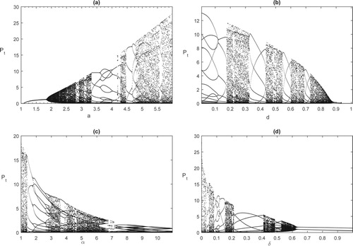20) ) there exist pest free periodic solutions which could be globally stable under certain conditions. However, the dynamics of these models could be very complex once the threshold conditions were no longer satisfied. To show this, we chose $a,d,\alpha ,$ and δ as the bifurcation parameters respectively; the bifurcation diagrams shown in Figure 2 reveal the complex dynamics of the model. The results indicate that system (4(4) $\begin{array}{r}\left\{\begin{array}{c}\left.\begin{array}{l}{P}_{t+1}=\frac{a{P}_t}{1+b{P}_t}{e}^{-\alpha N_t},\\ N_{t+1}=\beta P_t\left(1-e^{-\alpha N_t}\right)+d{N}_t,\end{array}\right\}t=1,2,\dots ,\\ \left.\begin{array}{l}{\omega }_{qk}=\frac{(1-d_1){\omega }_{q(k-1)}}{1-d_1{\omega }_{q(k-1)}},\\ P_{q{k}^{+}}=(1-d_1{\omega }_{qk})P_{qk},\\ N_{q{k}^{+}}=N_{qk}+{\delta }_k,\end{array}\right\}k=1,2,\dots ,\end{array}\right.\end{array}$(4) ) may exhibit complex dynamical behaviour such as period doubling bifurcations and multiple attractors co-existing for a wide range of parameters. Therefore, how do those complex dynamics affect the pest control when pesticide resistance develops? This question will be studied in the near future.

Figure 2. Bifurcation diagrams for model (4(4) $\begin{array}{r}\left\{\begin{array}{c}\left.\begin{array}{l}{P}_{t+1}=\frac{a{P}_t}{1+b{P}_t}{e}^{-\alpha N_t},\\ N_{t+1}=\beta P_t\left(1-e^{-\alpha N_t}\right)+d{N}_t,\end{array}\right\}t=1,2,\dots ,\\ \left.\begin{array}{l}{\omega }_{qk}=\frac{(1-d_1){\omega }_{q(k-1)}}{1-d_1{\omega }_{q(k-1)}},\\ P_{q{k}^{+}}=(1-d_1{\omega }_{qk})P_{qk},\\ N_{q{k}^{+}}=N_{qk}+{\delta }_k,\end{array}\right\}k=1,2,\dots ,\end{array}\right.\end{array}$(4) ) with different bifurcation parameters $a,d,alpha$, and δ. The baseline parameter values are as follows: $d_1=0.8,q=3,a=3.8,b=0.1,delta=0.1,\beta =0.4,d=0.1,\alpha =2$. (a) Bifurcation diagram for the density of the pest population with bifurcation parameter a; (b) Bifurcation diagram for the density of the pest population with bifurcation parameter d; (c) Bifurcation diagram for the density of the pest population with bifurcation parameter α; (d) Bifurcation diagram for the density of the pest population with bifurcation parameter δ.

Note that the evolution of pest resistance has been depicted in formula (2(2) $\begin{array}{rl}{\omega }_{kq}& =\frac{(1-d_1){\omega }_{(k-1)q}}{1-d_1{\omega }_{(k-1)q}},\\ {\omega }_{(k-1)q}& ={\omega }_{(k-1)q+1}=\cdots ={\omega }_{kq-1}.\end{array}$(2) ) within each generation, which is a simplification. In fact, the evolution of pesticide resistance could be modelled in different ways including evolution of resistance genes [25]. For example, if we assume that the pest resistance is determined by a single gene with two alleles R and S, and divide the pest population into three different types: homozygote resistant individuals RR, homozygote susceptibles SS and heterozygotes RS, then the evolution of the frequencies of the resistance allele in males and females can be modelled as follows [2, 4, 26]: $\begin{array}{rl}{p}_m(t+1)& =\frac{W_{m,RR}{p}_m\left(t\right)p_f\left(t\right)+0.5\left(W_{m,RS}\left(p_m\right(t\left)\right(1-p_f\left(t\right))+p_f(t\left)\right(1-p_m\left(t\right)\left)\right)\right)}{{\overline{W}}_m},\\ p_f(t+1)& =\frac{W_{f,RR}{p}_f\left(t\right)p_m\left(t\right)+0.5\left(W_{f,RS}\left(p_f\right(t\left)\right(1-p_m\left(t\right))+p_m(t\left)\right(1-p_f\left(t\right)\left)\right)\right)}{{\overline{W}}_f}\end{array}$ where $p_m$ and $p_f$ denote the frequencies of the resistance allele in males and in females, respectively. $W_{i,RR},W_{i,RS}$ ($i=m\left(male\right),f\left(female\right)$) are the fitness of male (female) RR type pest and fitness of male (female) RS type pest, and ${\overline{W}}_m,{\overline{W}}_f$ are the mean fitnesses of males and females, respectively. Important and interesting questions are how to combine the $p_m$ and $p_f$ into the dynamic equations for the pest and natural enemy populations, and how different evolution equations affect the dynamics of the models with pesticide resistance. Further, how to determine the trend of the evolution of pest resistance and set up the evolution of a pest resistance model considering the resistance gene and the effects of pesticide sprays on pest resistance, are questions to be addressed in future work.

In this paper, we assume that the population of pests are spatially homogenous. However, in many species, the distribution of populations in space is heterogeneous and such spatial heterogeneity has marked effects on the dynamics of host-parasitoid systems [1, 5, 12]. Thus, spatial heterogeneity should be modelled in population growth systems [30]. The question is how does spatial heterogeneity affect the pesticide resistance and pest control? In our future work, we will investigate this question also.

Disclosure statement

No potential conflict of interest was reported by the authors.

Additional information

Funding

This work was supported by the National Natural Science Foundation of China [Grant Nos.: 11871319, 61772017, 11631012] and by the Fundamental Research Funds for the Central Universities [Grant Nos.: GK201703003, GK201702013].

References

- V.A. Bailey, A.J. Nicholson, and E.J. Williams, Interaction between hosts and parasites when some host individuals are more difficult to find than others, J. Theoret. Biol. 3 (1962), pp. 1–18. doi: 10.1016/S0022-5193(62)80002-2
- S. Barbosa and I.M. Hastings, The importance of modelling the spread of insecticide resistance in a heterogeneous environment: the example of adding synergists to bed nets, Malaria J. 11 (2012), pp. 1–12. doi: 10.1186/1475-2875-11-258
- H.J. Barclay, Models for pest control using predator release, habitat management and pesticide release in combination, J. Appl. Ecol. 19 (1982), pp. 337–348. doi: 10.2307/2403471
- P.L. Birget and J.C. Koella, A genetic model of the effects of insecticide-treated bed nets on the evolution of insecticide-resistance, Evol. Med. Public Health 2015(1) (2015), pp. 205–215. doi: 10.1093/emph/eov019
- E. Broadhead and R.A. Cheke, Host spatial pattern, parasitoid interference and the modelling of the dynamics of Alaptus fusculus (Hym.:Mymaridae), a parasitoid of two Mesopsocus species (Psocoptera), J. Anim. Ecol. 44 (1975), pp. 767–793. doi: 10.2307/3718
- P. Debach, Biological Control by Natural Enemies, Cambridge University Press, London, 1974.
- Y. Dumont and J.M. Tchuenche, Mathematical studies on the sterile insect technique for the Chikungunya disease and Aedes albopictus, J. Math. Biol. 65 (2012), pp. 809–854. doi: 10.1007/s00285-011-0477-6
- M.L. Flint, Integrated pest management for walnuts, University of California Statewide Integrated Pest Management Project, Division of Agriculture and Natural Resources, 2nd ed., University of California, Oakland, CA, Publication 3270, 1987.
- G.P. Georghiou, Pest Resistance to Pesticides, Springer Science & Business Media, Boston, 2012.
- D.J. Greathead, Natural enemies of tropical locusts and grasshoppers: their impact and potential as biological control agents, in Biological Control of Locusts and Grasshoppers, C.J. Lomer and C. Prior, eds., C.A.B. International, Wallingford, UK, 1992, pp. 105–121.
- T.M. Ha, A Review on the development of integrated pest management and its integration in modern agriculture, Asian J. Agric. Food. Sci. 2 (2014), pp. 336–340.
- M.P. Hassell and R.M. May, Aggregation of predators and insect parasites and its effect on stability, J. Anim. Ecol. 43 (1974), pp. 567–94. doi: 10.2307/3384
- M.P. Hoffmann and A.C. Frodsham, Natural Enemies of Vegetable Insect Pests, Cooperative Extension, Cornell University, Ithaca, NY, 1993. 63.
- S.U. Karaağaç, Insecticide resistance, in Insecticides and Advances in Intergrated Pest Management, Perveen Farzana, ed., InTech Press, London, 2012, pp. 469–478.
- M.J. Kotchen, Incorporating Resistance in Pesticide Management: A Dynamic Regional Approach, Springer Verlag, New York, 1999, pp. 126–135.
- J.H. Liang and S.Y. Tang, Optimal dosage and economic threshold of multiple pesticide applications for pest control, Math. Comput. Model. 51 (2010), pp. 487–503. doi: 10.1016/j.mcm.2009.11.021
- J.H. Liang, S.Y. Tang, and R.A. Cheke, An integrated pest management model with delayed responses to pesticide applications and its threshold dynamics, Nonlinear Anal. 13 (2012), pp. 2352–2374. doi: 10.1016/j.nonrwa.2012.02.003
- J.H. Liang, S.Y. Tang, R.A. Cheke, and J.H. Wu, Adaptive release of natural enemies in a pest-natural enemy system with pesticide resistance, Bull. Math. Biol. 75 (2013), pp. 2167–2195. doi: 10.1007/s11538-013-9886-6
- J.H. Liang, S.Y. Tang, J.J. Nieto, and R.A. Cheke, Analytical methods for detecting pesticide switches with evolution of pesticide resistance, Math. Biosci. 245 (2013), pp. 249–257. doi: 10.1016/j.mbs.2013.07.008
- J.H. Liang, S.Y. Tang, R.A. Cheke, and J.H. Wu, Models for determining how many natural enemies to release inoculatively in combinations of biological and chemical control with pesticide resistance, J. Math. Anal. Appl. 422 (2015), pp. 1479–1503. doi: 10.1016/j.jmaa.2014.09.048
- J.H. Liang, S.Y. Tang, and R.A. Cheke, Beverton-Holt discrete pest management models with pulsed chemical control and evolution of pesticide resistance, Commun. Nonlinear Sci. Numer. Simul. 36 (2016), pp. 327–341. doi: 10.1016/j.cnsns.2015.12.014
- J.H. Liang, S.Y. Tang, and R.A. Cheke, Pure Bt-crop and mixed seed sowing strategies for optimal economic profit in the face of pest resistance to pesticides and Bt-corn, Appl. Math. Comput. 283 (2016), pp. 6–21.
- R. Lilley and C.A.M. Campbell, Biological, chemical and integrated control of two-spotted spider mite Tetranychus urticae on dwarf hops, Biocontrol Sci. Technol. 9 (1999), pp. 467–473. doi: 10.1080/09583159929433
- L. Mailleret and V. Lemesle, A note on semi-discrete modelling in the life sciences, Phil. Trans. R. Soc. A 367 (2009), pp. 4779–4799. doi: 10.1098/rsta.2009.0153
- R.M. May and A.P. Dobson, Population dynamics and the rate of evolution of pesticide resistance, in Pesticide Resistance: Strategies and Tactics for Management, National Academy Press, Washington D.C., 1986, pp. 170–193.
- C. Miller, A. Munoz, F. Pena, R. Rael, and A.A. Yakubu, To Bt or Not to Bt? Balancing spatial genetic heterogeneity to control the evolution of ostrinia nubilalis, 2001.
- P. Neuenschwander, H.R. Herren, I. Harpaz, D. Badulescu, and A.E. Akingbohungbe, Biological control of the cassava mealybug, Phenacoccus manihoti, by the exotic parasitoid Epidinocarsis lopezi in Africa [and discussion], Phil. Trans. R Soc. Lond. B 318 (1988), pp. 319–333. doi: 10.1098/rstb.1988.0012
- D.H. Oi, D.F. Williams, R.M. Pereira, P.M. Horton, T.S. Davis, A.H. Hyder, H.T. Bolton, B.C.Zeichner, S.D. Porter, L.A. Hoch, M.L. Boswell, and G. Williams, Combining biological and chemical controls for the management of red imported fire ants (Hymenoptera: Formicidae), Am. Entomol. 54 (2008), pp. 46–55. doi: 10.1093/ae/54.1.46
- D.W. Onstad, Insect Resistance Management: Biology, Economics, and Prediction, Academic Press, London, 2013.
- F. Paparella, C. Ferracini, A. Portaluri, A. Manzo, and A. Alma, Biological control of the chestnut gall wasp with T. Sinensis: A mathematical model, Ecol. Modell. 338 (2016), pp. 17–36. doi: 10.1016/j.ecolmodel.2016.07.023
- F.D. Parker, Management of pest populations by manipulating densities of both hosts and parasites through periodic releases, in Biological Control, Springer, US, 1971, pp. 365–376.
- D. Pimentel and M. Burgess, Environmental and economic costs of the application of pesticides primarily in the United States, in Integrated Pest Management, Springer, Netherlands, 2014.
- J.R. Ruberson, H. Nemoto, and Y. Hirose, Pesticides and conservation of natural enemies in pest management, Conser Biol Cont 20 (1998), pp. 207–220. doi: 10.1016/B978-012078147-8/50057-8
- S.Y. Tang and R.A. Cheke, Models for integrated pest control and their biological implications, Math. Biosci. 215 (2008), pp. 115–125. doi: 10.1016/j.mbs.2008.06.008
- S.Y. Tang, Y.N. Xiao, and R.A. Cheke, Multiple attractors of host-parasitoid models with integrated pest management strategies: Eradication, persistence and outbreak, Theoret. Popul. Biol. 73 (2008), pp. 181–197. doi: 10.1016/j.tpb.2007.12.001
- S.Y. Tang, Y.N. Xiao, and R.A. Cheke, Effects of predator and prey dispersal on success or failure of biological control, Bull. Math. Biol. 71 (2009), pp. 2025–2047. doi: 10.1007/s11538-009-9438-2
- S.Y. Tang, G.Y. Tang, and R.A. Cheke, Optimum timing for integrated pest management: Modelling rates of pesticide application and natural enemy releases, J. Theoret. Biol. 264 (2010), pp. 623–638. doi: 10.1016/j.jtbi.2010.02.034
- S.Y. Tang, J.H. Liang, Y.N. Xiao, and R.A. Cheke, Sliding bifurcations of Filippov two stage pest control models with economic thresholds, SIAM J. Appl. Math. 72 (2012), pp. 1061–1080. doi: 10.1137/110847020
- S.Y. Tang, J.H. Liang, Y.S. Tan, and R.A. Cheke, Threshold conditions for integrated pest management models with pesticides that have residual effects, J. Math. Biol. 66 (2013), pp. 1–35. doi: 10.1007/s00285-011-0501-x
- M.B. Thomas, Ecological approaches and the development of ‘truly integrated’ pest management, Proc. Natl. Acad. Sci. 96 (1999), pp. 5944–5951. doi: 10.1073/pnas.96.11.5944
- J.C. Van Lenteren, Integrated pest management in protected crops, in Integrated Pest Management, D. Dent, ed., Chapman & Hall, London, 1995, pp. 311–320.
- J.C. Van Lenteren, Measures of success in biological control of arthropods by augmentation of natural enemies, in Measures of Success in Biological Control, S. Wratten, and G. Gurr, eds., Kluwer Academic Publishers, Dordrecht, 2000, pp. 77–89.
- J.C. Van Lenteren and J. Woets, Biological and integrated pest control in greenhouses, Ann. Rev. Ent. 33 (1988), pp. 239–269. doi: 10.1146/annurev.en.33.010188.001323
- E. Zchori-Fein, R.T. Roush, and J.P. Sanderson, Potential for integration of biological and chemical control of greenhouse whitefly(Homoptera: Aleyrodidae) using Encarsia formosa (Hymenoptera: Aphelinidae) and abamectin, Env. Ent. 23 (1994), pp. 1277–1282. doi: 10.1093/ee/23.5.1277