Mathematical model to assess vaccination and effective contact rate impact in the spread of tuberculosis

ABSTRACT

The long and binding treatment of tuberculosis (TB) at least 6–8 months for the new cases, the partial immunity given by BCG vaccine, the loss of immunity after a few years doing that strategy of TB control via vaccination and treatment of infectious are not sufficient to eradicate TB. TB is an infectious disease caused by the bacillus Mycobacterium tuberculosis. Adults are principally attacked. In this work, we assess the impact of vaccination in the spread of TB via a deterministic epidemic model (SV ELI) (Susceptible, Vaccinated, Early latent, Late latent, Infectious). Using the Lyapunov–Lasalle method, we analyse the stability of epidemic system  (SV ELI) around the equilibriums (disease-free and endemic). The global asymptotic stability of the unique endemic equilibrium whenever ${\mathcal{R}}_0>1$ is proved, where ${\mathcal{R}}_0$ is the reproduction number. We prove also that when ${\mathcal{R}}_0$ is less than 1, TB can be eradicated. Numerical simulations, using some TB data found in the literature in relation with Cameroon, are conducted to approve analytic results, and to show that vaccination coverage is not sufficient to control TB, effective contact rate has a high impact in the spread of TB.

KEYWORDS:

• Effective contact rate
• vaccination
• tuberculosis
• basic reproduction number
• global stability

1. Introduction

Tuberculosis (TB) is one of the top 10 causes of death worldwide. It is caused by bacteria (Mycobacterium tuberculosis) that most often affects the lungs. TB is curable and preventable. TB is spread from person to person through the air. When people with lung TB cough, sneeze or spit, they propel the TB germs into the air. A person needs to inhale only a few of these germs to become infected. About one-third of the world population has latent TB, which means people have been infected by TB bacteria but are not (yet) ill with the disease and cannot transmit the disease. People infected with TB bacteria have a $10\mathrm{\%}$ lifetime risk of falling ill with TB. However, persons with compromised immune systems, such as people living with HIV, malnutrition or diabetes or people who use tobacco, have a much higher risk of falling ill. When a person develops active TB disease, the symptoms (such as cough, fever, night sweats or weight loss) may be mild for many months. This can lead to delays in seeking care and results in transmission of the bacteria to others. People with active TB can infect 10 other people through close contact over the course of a year. Without proper treatment, $45\mathrm{\%}$ of HIV-negative people with TB on average and nearly all HIV-positive people with TB will die [20]. The best estimates for 2015 are that there were 10.4 million new TB cases (including 1.2 million among HIV-positive people), of which 5.9 million were among men, 3.5 million among women and 1.0 million among children. Overall, $90\mathrm{\%}$ of cases were adults and 10$\mathrm{\%}$ children, and the male/female ratio was $1.6/1$. People living with HIV accounted for 1.2 million (11$\mathrm{\%}$) of all new TB cases [20]. The theme ‘End the global TB’ has been decided by the World Health Organization (WHO) and it covers the period 2016–2035 and the overall goal is to end the global TB epidemic, denned as around 10 new cases per 100,000 population per year. As part of the necessary multidisciplinary research approach, mathematical models have been extensively used to provide a framework for understanding TB transmission dynamics and control strategies of the infection spread in the host population. In the literature, considerable works can be found on the mathematical modelling and to assess the impact of some control strategies (like vaccination and treatment of infectious) to fight TB [4,14,17]. Some of these works have been conducted to explore the impact of HIV/AIDS in the spread of TB [18]. Arthur et al. study social and cultural factors in the successful control of TB.

This paper deals with the weakness of the TB strategy through mass vaccination and the multidimensional poverty in the spread of TB via a SV ELI transmission model. Individuals are classified as one of susceptible S, vaccinated V, earlier latent E, late latent L and infectious I. The model is based on a standard SV ELI model [9], but allows that susceptible individuals may be given an imperfect vaccine that reduces their susceptibility to the disease. Since we consider a leaky vaccine, the V-compartment of vaccinated individuals is considered as a susceptible compartment, and thus we are dealing with a differential susceptibility system with bilinear mass action as in Hyman and Li [10]. However, we include one-way flow between these two compartments due to vaccination making the model studied here distinct from the model of Guo et al. [9]. Using the Lyapunov–LaSalle method, we fully resolve the global dynamics of the model for the full parameter space. We demonstrate that the model exhibits threshold behaviour with a globally stable disease-free equilibrium (DFE) if the basic reproduction number is less than unity and a globally stable endemic equilibrium if the basic reproduction number is greater than unity. In order to study the stability of a positive endemic equilibrium state, we use Lyapunov's direct method and LaSalle's Invariance Principle with a Lyapunov function of Goh–Volterra type: $V(x_1,x_2,\dots ,x_n)=\sum _i{A}_i(x_i-x_i^{\ast }\ln x_i),$ where $A_1,\dots ,A_n$ are constants, $x_i$ is the population of ith compartment and $x_i^{\ast }$ is the equilibrium level. Lyapunov functions of this type have also proven to be useful for Lotka–Voltera predator–prey systems [1], and it appears that they can be useful for more complex compartmental epidemic.

The manuscript is organized as follows. In the next section, we formulate the model and derive its basic properties. In Section 3, the reproduction number is derived, and the stability of DFE is established. Existence, uniqueness and stability of an endemic equilibrium are shown in Section 4. While Section 5 is devoted to the numerical simulations which will be done with some Cameroon data collected at Jamot hospital. Section 6 concludes the paper and provides a discussion for future and ongoing works.

2. The model formulation

2.1. Model description

When first infected with TB bacteria, a person typically goes through a latent, asymptomatic and non-infectious period during which the body's immune system fights the TB bacteria. There are two distinct stages of the latent TB infection. During the first 2 years, the risk of developing active disease is much higher, whereas during the later stage, the progression to active disease is much slower.

Using a compartmental approach, the total host population can be partitioned into five compartments: susceptible individuals $\left(S\right)$, vaccinated $\left(V\right)$, early latent $\left(E\right)$ and late latent $\left(L\right)$ individuals, and individuals with active TB disease $\left(I\right)$. $S\left(t\right),V\left(t\right),E\left(t\right),L\left(t\right)$ and $I\left(t\right)$ denote the density of populations in the four corresponding compartments at time t. Only individuals in compartment I are infectious, and new infections result on the one hand from contacts between a susceptible and an infectious individual, with an incidence rate $\beta SI$ and on the other hand from contacts between a vaccinated and infectious individual, with an incidence $\theta \beta VI$, due to the fact that the vaccine doesn't confer a total immunity, but Vaccination reduces the risk of infection by a factor $\theta \in (0,1)$ and the efficacy of the vaccine is $1-\theta$. The per capita death rates for susceptible, vaccinated, early latent, late latent and infectious individuals are ${\mu }_S$, ${\mu }_V$, ${\mu }_E$, ${\mu }_L$ and ${\mu }_I$ respectively. Once infected, individuals progress through the early latent stage with an average rate ω. A fraction $p(0<p\le 1)$ of these individuals progress directly to the active TB stage, and the remaining 1−p fraction progresses to the late latent stage. Once there, the rate of progression to active disease is at a lower rate ν. The recruitment only makes into the susceptible class with the constant rate Λ. ϵ is the vaccination coverage rate. The above-mentioned biological descriptions lead to the following system of nonlinear differential equations whose flow diagram, state variables and parameters are given in Figure 1 and Table 1, respectively: (1) $\begin{array}{rl}\dot{S}& =\mathrm{\Lambda }-\beta SI-({\mu }_S+\epsilon )S,\\ \dot{V}& =\epsilon S-{\mu }_{V}V-\theta \beta VI,\\ \dot{E}& =\beta SI+\theta \beta VI-({\mu }_E+\omega )E,\\ \dot{L}& =(1-p)\omega E-({\mu }_L+\nu )L,\\ \dot{I}& =p\omega E+\nu L-{\mu }_{I}I,\\ N& =S+V+E+L+I\end{array}$(1) with initial conditions $\left(S\right(0),V(0),E(0),L(0),I(0\left)\right)\in {\mathbb{R}}_{+}^5$.

Figure 1. Schema of the compartmental model.

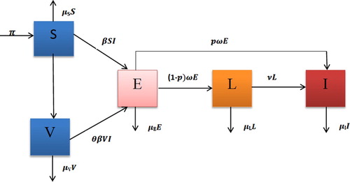
Table 1. Description of state variables and parameters of model (1(1) $\begin{array}{rl}\dot{S}& =\mathrm{\Lambda }-\beta SI-({\mu }_S+\epsilon )S,\\ \dot{V}& =\epsilon S-{\mu }_{V}V-\theta \beta VI,\\ \dot{E}& =\beta SI+\theta \beta VI-({\mu }_E+\omega )E,\\ \dot{L}& =(1-p)\omega E-({\mu }_L+\nu )L,\\ \dot{I}& =p\omega E+\nu L-{\mu }_{I}I,\\ N& =S+V+E+L+I\end{array}$(1) ).

Variables	Description
S	Susceptible human individuals
V	Vaccinated human individuals
E	Earlier latent
L	Later latent
I	TB-infected human individuals
Parameters	Description
Λ	Recruitment of susceptible
ϵ	Vaccination coverage rate
ω	Progression rate to latent earlier stage
β	Effective contact rate
$1-\theta$	Vaccine efficacy
${\mu }_S$, ${\mu }_V$	Natural death rate of human individuals
${\mu }_E$, ${\mu }_L$,	Natural death rate latent individuals
${\mu }_I$	Death rate for I including natural and disease-caused death
p	Fraction of individuals who progress directly in TB active stage
1−p	Progression fraction to the late latent stage
ν	Progression rate to active disease

2.2. Basic properties

For the TB transmission model (1(1) $\begin{array}{rl}\dot{S}& =\mathrm{\Lambda }-\beta SI-({\mu }_S+\epsilon )S,\\ \dot{V}& =\epsilon S-{\mu }_{V}V-\theta \beta VI,\\ \dot{E}& =\beta SI+\theta \beta VI-({\mu }_E+\omega )E,\\ \dot{L}& =(1-p)\omega E-({\mu }_L+\nu )L,\\ \dot{I}& =p\omega E+\nu L-{\mu }_{I}I,\\ N& =S+V+E+L+I\end{array}$(1) ) to be epidemiological meaningful, it is important to prove that all state variables are non-negative at all time. That is, solutions of the system (1(1) $\begin{array}{rl}\dot{S}& =\mathrm{\Lambda }-\beta SI-({\mu }_S+\epsilon )S,\\ \dot{V}& =\epsilon S-{\mu }_{V}V-\theta \beta VI,\\ \dot{E}& =\beta SI+\theta \beta VI-({\mu }_E+\omega )E,\\ \dot{L}& =(1-p)\omega E-({\mu }_L+\nu )L,\\ \dot{I}& =p\omega E+\nu L-{\mu }_{I}I,\\ N& =S+V+E+L+I\end{array}$(1) ) with non-negative initial data will remain non-negative for all time t>0.

Theorem 2.1

Let the initial data be $S\left(0\right),$ $V\left(0\right),$ $E\left(0\right),$ $L\left(0\right),$ $I\left(0\right)$ be non-negative. Then, the solutions $(S,V,E,L,I)$ of model (1(1) $\begin{array}{rl}\dot{S}& =\mathrm{\Lambda }-\beta SI-({\mu }_S+\epsilon )S,\\ \dot{V}& =\epsilon S-{\mu }_{V}V-\theta \beta VI,\\ \dot{E}& =\beta SI+\theta \beta VI-({\mu }_E+\omega )E,\\ \dot{L}& =(1-p)\omega E-({\mu }_L+\nu )L,\\ \dot{I}& =p\omega E+\nu L-{\mu }_{I}I,\\ N& =S+V+E+L+I\end{array}$(1) ) are positive and bounded for all $t>0,$ whenever they exists.

Proof.

Suppose $S\left(0\right)\ge 0$. The first equation of system (1(1) $\begin{array}{rl}\dot{S}& =\mathrm{\Lambda }-\beta SI-({\mu }_S+\epsilon )S,\\ \dot{V}& =\epsilon S-{\mu }_{V}V-\theta \beta VI,\\ \dot{E}& =\beta SI+\theta \beta VI-({\mu }_E+\omega )E,\\ \dot{L}& =(1-p)\omega E-({\mu }_L+\nu )L,\\ \dot{I}& =p\omega E+\nu L-{\mu }_{I}I,\\ N& =S+V+E+L+I\end{array}$(1) ) can be written as $\frac{\mathrm{d}}{\mathrm{d}t}\left[S\right(t\left)\rho \right(t\left)\right]=\mathrm{\Lambda }\rho \left(t\right),$ where $\rho \left(t\right)=\exp \left({\int }_0^t\right[\beta I\left(s\right)+{\mu }_S+\epsilon \left]\mathrm{d}s\right)>0$ is the integrating factor. Hence, integrating this last relation with respect to t, we have $S\left(t\right)\rho \left(t\right)-S\left(0\right)={\int }_0^t\mathrm{\Lambda }\rho \left(s\right)\mathrm{d}s,$ so that the division of both side by $\rho \left(t\right)$ yields $S\left(t\right)=\left[S\left(0\right)+{\int }_0^t\mathrm{\Lambda }\rho \left(s\right)\mathrm{d}s\right]\times {\rho }^{-1}\left(t\right)>0.$ The same arguments can be used to prove that $V\left(t\right)>0$ and $E\left(t\right)$, $L\left(t\right)$, $I\left(t\right)\ge 0$ for all t>0.

Furthermore, let N=S+V +E+L+I. Then, $\begin{array}{rl}\dot{N}\left(t\right)& =\dot{S}+\dot{V}+\dot{E}+\dot{L}+\dot{I},\\ & =\mathrm{\Lambda }-{\mu }_{S}S-{\mu }_{V}V-{\mu }_{E}E-{\mu }_{L}L-{\mu }_{I}I,\\ & \le \mathrm{\Lambda }-\mu N,\end{array}$ where $\mu =min\{{\mu }_S,{\mu }_V,{\mu }_E,{\mu }_L,{\mu }_I\}$. This implies that $\underset{t\to +\mathrm{\infty }}{lim}supN\left(t\right)\le \frac{\mathrm{\Lambda }}{\mu }.$ Also from (1(1) $\begin{array}{rl}\dot{S}& =\mathrm{\Lambda }-\beta SI-({\mu }_S+\epsilon )S,\\ \dot{V}& =\epsilon S-{\mu }_{V}V-\theta \beta VI,\\ \dot{E}& =\beta SI+\theta \beta VI-({\mu }_E+\omega )E,\\ \dot{L}& =(1-p)\omega E-({\mu }_L+\nu )L,\\ \dot{I}& =p\omega E+\nu L-{\mu }_{I}I,\\ N& =S+V+E+L+I\end{array}$(1) ), we have $\dot{S}\le \mathrm{\Lambda }-(\epsilon +{\mu }_S)\text{and}\dot{\phantom{a}}V\le \frac{\mathrm{\Lambda }\epsilon }{\epsilon +{\mu }_S}-{\mu }_{V}V.$ Thus $\underset{t\to +\mathrm{\infty }}{lim}supS\left(t\right)\le \frac{\mathrm{\Lambda }}{\epsilon +{\mu }_S}\text{and}\underset{t\to +\mathrm{\infty }}{lim}supV\left(t\right)\le \frac{\mathrm{\Lambda }}{\epsilon {\mu }_V(\epsilon +{\mu }_S)}.$ This completes the proof.

Combining Theorem 2.1 with the trivial existence and uniqueness of a local solution for the model (1(1) $\begin{array}{rl}\dot{S}& =\mathrm{\Lambda }-\beta SI-({\mu }_S+\epsilon )S,\\ \dot{V}& =\epsilon S-{\mu }_{V}V-\theta \beta VI,\\ \dot{E}& =\beta SI+\theta \beta VI-({\mu }_E+\omega )E,\\ \dot{L}& =(1-p)\omega E-({\mu }_L+\nu )L,\\ \dot{I}& =p\omega E+\nu L-{\mu }_{I}I,\\ N& =S+V+E+L+I\end{array}$(1) ), we have established the following theorem which ensures the mathematical and biological well-posedness of system (1(1) $\begin{array}{rl}\dot{S}& =\mathrm{\Lambda }-\beta SI-({\mu }_S+\epsilon )S,\\ \dot{V}& =\epsilon S-{\mu }_{V}V-\theta \beta VI,\\ \dot{E}& =\beta SI+\theta \beta VI-({\mu }_E+\omega )E,\\ \dot{L}& =(1-p)\omega E-({\mu }_L+\nu )L,\\ \dot{I}& =p\omega E+\nu L-{\mu }_{I}I,\\ N& =S+V+E+L+I\end{array}$(1) ).

Theorem 2.2

The dynamics of model (1(1) $\begin{array}{rl}\dot{S}& =\mathrm{\Lambda }-\beta SI-({\mu }_S+\epsilon )S,\\ \dot{V}& =\epsilon S-{\mu }_{V}V-\theta \beta VI,\\ \dot{E}& =\beta SI+\theta \beta VI-({\mu }_E+\omega )E,\\ \dot{L}& =(1-p)\omega E-({\mu }_L+\nu )L,\\ \dot{I}& =p\omega E+\nu L-{\mu }_{I}I,\\ N& =S+V+E+L+I\end{array}$(1) ) is a dynamical system in the biological feasible compact set $\mathrm{\Gamma }=\left\{(S,V,E,L,I)\in {\mathbb{R}}_{+}^5:0\le S\le \frac{\mathrm{\Lambda }}{\epsilon +{\mu }_S},V\le \frac{\mathrm{\Lambda }\epsilon }{{\mu }_V(\epsilon +{\mu }_S)},N\le \frac{\mathrm{\Lambda }}{\mu }\right\}.$

3. Basic reproduction number ${\mathcal{R}}_0$ and DFE

3.1. Computation of ${\mathcal{R}}_0$

It is easy to check that model (1(1) $\begin{array}{rl}\dot{S}& =\mathrm{\Lambda }-\beta SI-({\mu }_S+\epsilon )S,\\ \dot{V}& =\epsilon S-{\mu }_{V}V-\theta \beta VI,\\ \dot{E}& =\beta SI+\theta \beta VI-({\mu }_E+\omega )E,\\ \dot{L}& =(1-p)\omega E-({\mu }_L+\nu )L,\\ \dot{I}& =p\omega E+\nu L-{\mu }_{I}I,\\ N& =S+V+E+L+I\end{array}$(1) ) has always a DFE $P_0=(S_0,V_0,0,0,0)$ where $S_0=\frac{\mathrm{\Lambda }}{{\mu }_S+\epsilon }\text{and}{V}_0=\frac{\mathrm{\Lambda }\epsilon }{{\mu }_V(\epsilon +{\mu }_S)},$ which is obtained by setting the right-hand side of system (1(1) $\begin{array}{rl}\dot{S}& =\mathrm{\Lambda }-\beta SI-({\mu }_S+\epsilon )S,\\ \dot{V}& =\epsilon S-{\mu }_{V}V-\theta \beta VI,\\ \dot{E}& =\beta SI+\theta \beta VI-({\mu }_E+\omega )E,\\ \dot{L}& =(1-p)\omega E-({\mu }_L+\nu )L,\\ \dot{I}& =p\omega E+\nu L-{\mu }_{I}I,\\ N& =S+V+E+L+I\end{array}$(1) ) to zero.

A key quantity in classic epidemiological models is the basic reproduction number, denoted by ${\mathcal{R}}_0$. It is a useful threshold in the study of a disease for predicting a disease outbreak and for evaluating the control strategies. Following [7], the next generation approach is used to calculate ${\mathcal{R}}_0$. Let $\begin{array}{rl}& \mathcal{F}=(\beta SI+\theta \beta VI,(1-p)\omega E,p\omega E{)}^{\mathrm{T}}\text{and}\\ & \mathcal{G}=(-({\mu }_E+\omega )E,-({\mu }_L+\nu )L,\nu L-{\mu }_{I}I{)}^{\mathrm{T}}\end{array}$ be the vector of new generated infected and the vector of transfers between compartments, respectively. The Jacobian matrices of $\mathcal{F}$ and $\mathcal{G}$ at the DFE $P_0$ are $F=\left(\begin{array}{ccc}0& 0& \beta S_0+\theta \beta V_0\\ (1-p)\omega & 0& 0\\ p\omega & 0& 0\end{array}\right)\text{and}G=\left(\begin{array}{ccc}-({\mu }_E+\omega )& 0& 0\\ 0& -({\mu }_L+\nu )& 0\\ 0& \nu & -{\mu }_I\end{array}\right).$ Thanks to [7], the associated basic reproduction number ${\mathcal{R}}_0$ of (1(1) $\begin{array}{rl}\dot{S}& =\mathrm{\Lambda }-\beta SI-({\mu }_S+\epsilon )S,\\ \dot{V}& =\epsilon S-{\mu }_{V}V-\theta \beta VI,\\ \dot{E}& =\beta SI+\theta \beta VI-({\mu }_E+\omega )E,\\ \dot{L}& =(1-p)\omega E-({\mu }_L+\nu )L,\\ \dot{I}& =p\omega E+\nu L-{\mu }_{I}I,\\ N& =S+V+E+L+I\end{array}$(1) ) is the spectral radius of the next generation matrix $-F{G}^{-1}$. That is (2) ${\mathcal{R}}_0=\frac{\beta \mathrm{\Lambda }\omega (\nu +p{\mu }_L)({\mu }_V+\theta \epsilon )}{{\mu }_I{\mu }_V(\epsilon +{\mu }_S)({\mu }_E+\omega )({\mu }_L+\nu )}.$(2)

3.2. Sensitivity analysis

We carried out sensitivity analysis to determine the model robustness to parameter values. This is a tool to identify the most influential parameters in determining model dynamics [2,11]. A latin Hypercupe Sampling (LHS) scheme [12] samples 1000 values for each input parameter using a uniform distribution over the range of ecologically realistic values is given in Figure 2 with descriptions and references given in Table 2. Using the system of differential equations that describe (1(1) $\begin{array}{rl}\dot{S}& =\mathrm{\Lambda }-\beta SI-({\mu }_S+\epsilon )S,\\ \dot{V}& =\epsilon S-{\mu }_{V}V-\theta \beta VI,\\ \dot{E}& =\beta SI+\theta \beta VI-({\mu }_E+\omega )E,\\ \dot{L}& =(1-p)\omega E-({\mu }_L+\nu )L,\\ \dot{I}& =p\omega E+\nu L-{\mu }_{I}I,\\ N& =S+V+E+L+I\end{array}$(1) ), 5000 model simulations are performed by randomly pairing sampled values for all LHS parameters. Partial Rank Correlation Coefficients (PRCC) and corresponding p-values between ${\mathcal{R}}_0$ and each parameter are computed. An output is assumed sensitive to an input if the corresponding PRCC is less than $-0.50$ or greater than $+0.50$, and the corresponding p-value is less than $5\mathrm{\%}$.

Figure 2. Sensitivity analysis between ${\mathcal{R}}_0$ and each parameter.

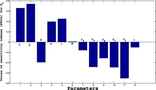
Table 2. Values and ranges of the parameters of model (1(1) $\begin{array}{rl}\dot{S}& =\mathrm{\Lambda }-\beta SI-({\mu }_S+\epsilon )S,\\ \dot{V}& =\epsilon S-{\mu }_{V}V-\theta \beta VI,\\ \dot{E}& =\beta SI+\theta \beta VI-({\mu }_E+\omega )E,\\ \dot{L}& =(1-p)\omega E-({\mu }_L+\nu )L,\\ \dot{I}& =p\omega E+\nu L-{\mu }_{I}I,\\ N& =S+V+E+L+I\end{array}$(1) ).

Parameters	Values	Range	Source
Λ	10	$[1;20]$	[15,16]
β	Variable	$[1e-5;1e-1]$	Assumed
θ	0.50	$[0.2;0.90]$	[6]
ω	0.0645	$[1e-2;1e-1]$	[8]
ν	0.00375	$[2e-3;1e-2]$	[3]
p	1.14e−3	$[6.70e-5;1.97e-3]$	[13]
${\mu }_S$, ${\mu }_V$, ${\mu }_E$, ${\mu }_L$	0.01874	$[1e-2;1e-1]$	[13]
${\mu }_I$	0.1577	$[1e-2;5e-1]$	[13]
ϵ	Variable	$[0.1,0.98]$	Assumed

From Figure 2, we can identify some parameters that strongly influence the dynamics of TB infection, namely Λ, β, θ, ω, ν, ${\mu }_V$, ${\mu }_L$ and ${\mu }_I$. Parameters Λ, β, ω, ν and p have a positive influence on the basic reproduction number ${\mathcal{R}}_0$, that is, an increase in these parameters implies an increase in ${\mathcal{R}}_0$. While parameters θ, ${\mu }_S$, ${\mu }_V$, ${\mu }_E$,${\mu }_L$, ${\mu }_I$ and ϵ have a negative influence on the basic reproduction number ${\mathcal{R}}_0$, that is, an increase in these parameters implies a decrease in ${\mathcal{R}}_0$. Thus, from this sensitivity analysis, the following suggestions are made:

1. Quarantining infected individuals could be an effective control measure against the growing of TB infection because it reduces the value of contact rate β.

2. An increase of screening of latent individuals (earlier and later latent) may play an important role in minimizing the size of infected individuals by reducing the progression rates ω and ν.

3. Also, an increase of the effectiveness vaccination rate and vaccination coverage rate is another good control tool against TB infection because it helps increasing the values of θ and ϵ.

3.3. Stability of the DFE

Using Theorem 2 in [7], the following result is straightforward.

Lemma 3.1

The DFE $P_0$ of model (1(1) $\begin{array}{rl}\dot{S}& =\mathrm{\Lambda }-\beta SI-({\mu }_S+\epsilon )S,\\ \dot{V}& =\epsilon S-{\mu }_{V}V-\theta \beta VI,\\ \dot{E}& =\beta SI+\theta \beta VI-({\mu }_E+\omega )E,\\ \dot{L}& =(1-p)\omega E-({\mu }_L+\nu )L,\\ \dot{I}& =p\omega E+\nu L-{\mu }_{I}I,\\ N& =S+V+E+L+I\end{array}$(1) ) is locally asymptotically stable whenever ${\mathcal{R}}_0<1$ and unstable otherwise.

Biologically speaking, Lemma 3.1 implies that infected can be eliminated if the initial sizes are in the basin of attraction of the DFE $P_0$. Thus the infected population can be effectively controlled if ${\mathcal{R}}_0<1$. To ensure that the effective control of the infected population is independent of the initial size of the human population, a global asymptotic stability result must be established for the DFE.

Theorem 3.1

If ${\mathcal{R}}_0\le 1,$ then the DFE is globally asymptotically stable.

Proof.

Let $X=(S,V,E,L,I{)}^T$ and consider a Lyapunov function, $\mathcal{V}\left(X\right)=\omega (p{\mu }_L+\nu )E+\nu ({\mu }_E+\omega )L+({\mu }_E+\omega )({\mu }_L+\nu )I.$ Direct calculation leads to $\begin{array}{rl}\dot{\mathcal{V}}& =\omega (p{\mu }_L+\nu )\dot{E}+\nu ({\mu }_E+\omega )\dot{L}+({\mu }_E+\omega )({\mu }_L+\nu )\dot{I},\\ & =\omega (p{\mu }_L+\nu )(\beta SI+\theta \beta VI-({\mu }_E+\omega \left)E\right)+\nu ({\mu }_E+\omega )\left(\right(1-p)\omega E-({\mu }_L+\nu \left)L\right)\\ & +({\mu }_E+\omega )({\mu }_L+\nu )(p\omega E+\nu L-{\mu }_{I}T),\\ & =\omega (\nu +p{\mu }_L)(\beta SI+\theta \beta VI)-{\mu }_I({\mu }_E+\omega )({\mu }_L+\nu )I,\\ & ={\mu }_I({\mu }_E+\omega )({\mu }_L+\nu )\left[\frac{\omega \beta (\nu +p{\mu }_L)(S+\theta V)}{{\mu }_I({\mu }_E+\omega )({\mu }_L+\nu )}-1\right]I.\end{array}$ Therefore, $\begin{array}{rl}\dot{\mathcal{V}}& \le {\mu }_I({\mu }_E+\omega )({\mu }_L+\nu )\left[\frac{\omega \beta (\nu +p{\mu }_L)(S^{\ast }+\theta V^{\ast })}{{\mu }_I({\mu }_E+\omega )({\mu }_L+\nu )}-1\right]I,\text{since}S,V\in \mathrm{\Gamma },\\ & \le {\mu }_I({\mu }_E+\omega )({\mu }_L+\nu )[{\mathcal{R}}_0-1]I\le 0,\text{whenever}{\mathcal{R}}_0\le 1.\end{array}$ Furthermore, $\dot{\mathcal{V}}=0\leftrightarrow I=0\text{or}S=S_0,V=V_0\text{and}{\mathcal{R}}_0=1.$ Thus the largest invariant set $\mathcal{H}$ such as $\mathcal{H}\subset \{X\in \mathrm{\Omega }/\dot{\mathcal{V}}(X)=0\}$ is the singleton $\left\{P_0\right\}$. By LaSalle's Invariance Principle, $P_0$ is globally asymptotically stable in Γ, completing the proof.

Theorem 3.1 completely determines the global dynamics of model (1(1) $\begin{array}{rl}\dot{S}& =\mathrm{\Lambda }-\beta SI-({\mu }_S+\epsilon )S,\\ \dot{V}& =\epsilon S-{\mu }_{V}V-\theta \beta VI,\\ \dot{E}& =\beta SI+\theta \beta VI-({\mu }_E+\omega )E,\\ \dot{L}& =(1-p)\omega E-({\mu }_L+\nu )L,\\ \dot{I}& =p\omega E+\nu L-{\mu }_{I}I,\\ N& =S+V+E+L+I\end{array}$(1) ) in Γ when ${\mathcal{R}}_0\le 1$. It establishes the basic reproduction number ${\mathcal{R}}_0$ as a sharp threshold parameter. Namely, if ${\mathcal{R}}_0>1$, all solutions in the feasible region converge to the DFE $P_0$, and the TB will die out from the population irrespective of the initial conditions. If ${\mathcal{R}}_0>1$, $P_0$ is unstable and the system is uniformly persistent, and a TB epidemic will always become endemic.

4. Endemic equilibrium and its stability

4.1. Existence and uniqueness

An equilibrium $P^{\ast }=(S^{\ast },V^{\ast },E^{\ast },L^{\ast },I^{\ast })$ of model (1(1) $\begin{array}{rl}\dot{S}& =\mathrm{\Lambda }-\beta SI-({\mu }_S+\epsilon )S,\\ \dot{V}& =\epsilon S-{\mu }_{V}V-\theta \beta VI,\\ \dot{E}& =\beta SI+\theta \beta VI-({\mu }_E+\omega )E,\\ \dot{L}& =(1-p)\omega E-({\mu }_L+\nu )L,\\ \dot{I}& =p\omega E+\nu L-{\mu }_{I}I,\\ N& =S+V+E+L+I\end{array}$(1) ) need to satisfy the following equations: (3) $\begin{array}{rl}\mathrm{\Lambda }-\beta S^{\ast }{I}^{\ast }-({\mu }_S+\epsilon )S^{\ast }& =0,\\ \epsilon S^{\ast }-{\mu }_V{V}^{\ast }-\theta \beta V^{\ast }{I}^{\ast }& =0,\\ \beta S^{\ast }{I}^{\ast }+\theta \beta V^{\ast }{I}^{\ast }-({\mu }_E+\omega )E^{\ast }& =0,\\ (1-p)\omega E^{\ast }-({\mu }_L+\nu )L^{\ast }& =0,\\ p\omega E^{\ast }+\nu L^{\ast }-{\mu }_I{I}^{\ast }& =0.\end{array}$(3) Solving (3(3) $\begin{array}{rl}\mathrm{\Lambda }-\beta S^{\ast }{I}^{\ast }-({\mu }_S+\epsilon )S^{\ast }& =0,\\ \epsilon S^{\ast }-{\mu }_V{V}^{\ast }-\theta \beta V^{\ast }{I}^{\ast }& =0,\\ \beta S^{\ast }{I}^{\ast }+\theta \beta V^{\ast }{I}^{\ast }-({\mu }_E+\omega )E^{\ast }& =0,\\ (1-p)\omega E^{\ast }-({\mu }_L+\nu )L^{\ast }& =0,\\ p\omega E^{\ast }+\nu L^{\ast }-{\mu }_I{I}^{\ast }& =0.\end{array}$(3) ) for $P^{\ast }$ yields (4) $\begin{array}{rl}{S}^{\ast }& =\frac{\mathrm{\Lambda }}{\beta I^{\ast }+\epsilon +{\mu }_S},V^{\ast }=\frac{\mathrm{\Lambda }\epsilon }{(\beta I^{\ast }+\epsilon +{\mu }_S)({\mu }_V+\theta \beta I^{\ast })},\\ E^{\ast }& =\frac{{\mu }_I({\mu }_L+\nu )}{\omega (p{\mu }_L+\nu )}{I}^{\ast },L^{\ast }=\frac{(1-p)\omega {\mu }_I({\mu }_L+\nu )}{\omega (p{\mu }_L+\nu )({\mu }_L+\nu )}{I}^{\ast }.\end{array}$(4) After substituting (4(4) $\begin{array}{rl}{S}^{\ast }& =\frac{\mathrm{\Lambda }}{\beta I^{\ast }+\epsilon +{\mu }_S},V^{\ast }=\frac{\mathrm{\Lambda }\epsilon }{(\beta I^{\ast }+\epsilon +{\mu }_S)({\mu }_V+\theta \beta I^{\ast })},\\ E^{\ast }& =\frac{{\mu }_I({\mu }_L+\nu )}{\omega (p{\mu }_L+\nu )}{I}^{\ast },L^{\ast }=\frac{(1-p)\omega {\mu }_I({\mu }_L+\nu )}{\omega (p{\mu }_L+\nu )({\mu }_L+\nu )}{I}^{\ast }.\end{array}$(4) ) into the third equation of (3(3) $\begin{array}{rl}\mathrm{\Lambda }-\beta S^{\ast }{I}^{\ast }-({\mu }_S+\epsilon )S^{\ast }& =0,\\ \epsilon S^{\ast }-{\mu }_V{V}^{\ast }-\theta \beta V^{\ast }{I}^{\ast }& =0,\\ \beta S^{\ast }{I}^{\ast }+\theta \beta V^{\ast }{I}^{\ast }-({\mu }_E+\omega )E^{\ast }& =0,\\ (1-p)\omega E^{\ast }-({\mu }_L+\nu )L^{\ast }& =0,\\ p\omega E^{\ast }+\nu L^{\ast }-{\mu }_I{I}^{\ast }& =0.\end{array}$(3) ), we obtain the following equation for $I^{\ast }$ $\frac{\beta \mathrm{\Lambda }(\theta \beta I^{\ast }+\theta \epsilon +{\mu }_V)}{(\beta I^{\ast }+\epsilon +{\mu }_S)({\mu }_V+\theta \beta I^{\ast })}-\frac{{\mu }_I({\mu }_E+\omega )({\mu }_L+\nu )}{\omega (p{\mu }_L+\nu )}=0.$ Let $f\left(x\right)=\frac{\beta \mathrm{\Lambda }(\theta \beta x+\theta \epsilon +{\mu }_V)}{(\beta x+\epsilon +{\mu }_S)({\mu }_V+\theta \beta x)}-\frac{{\mu }_I({\mu }_E+\omega )({\mu }_L+\nu )}{\omega (p{\mu }_L+\nu )}.$ It can be easily seen that $f^{\prime }\left(x\right)<0$, $\underset{x\to +\mathrm{\infty }}{lim}f\left(x\right)<0$ and $f\left(0\right)=\left(\right({\mu }_I({\mu }_E+\omega )({\mu }_L+\nu )\left)/\omega (p{\mu }_L+\nu )\right)({\mathcal{R}}_0-1)$, so that if ${\mathcal{R}}_0>1$, then $f\left(0\right)>0$. Therefore, there exists a unique positive root of the equation $f\left(x\right)=0$ only when $R_0>1$. The following result is immediate.

Theorem 4.1

The model (1(1) $\begin{array}{rl}\dot{S}& =\mathrm{\Lambda }-\beta SI-({\mu }_S+\epsilon )S,\\ \dot{V}& =\epsilon S-{\mu }_{V}V-\theta \beta VI,\\ \dot{E}& =\beta SI+\theta \beta VI-({\mu }_E+\omega )E,\\ \dot{L}& =(1-p)\omega E-({\mu }_L+\nu )L,\\ \dot{I}& =p\omega E+\nu L-{\mu }_{I}I,\\ N& =S+V+E+L+I\end{array}$(1) ) has a unique endemic equilibrium $P^{\ast },$ whenever ${\mathcal{R}}_0>1$.

4.2. Stability analysis of the endemic equilibrium

In this section, we further establish that all solutions in the interior of the feasible region converge to the unique endemic equilibrium $P^{\ast }$ if ${\mathcal{R}}_0>1$. Therefore, TB will persist at the endemic equilibrium level. The proof is accomplished by constructing a global Lyapunov function. Lyapunov functions of Goh–Volterra type have been used in the literature, see [9,11].

Theorem 4.2

If ${\mathcal{R}}_0>1,$ then the endemic equilibrium point $P^{\ast }=(S^{\ast },V^{\ast },E^{\ast },L^{\ast },I^{\ast }{)}^T$ is globally asymptotically stable in Γ.

Proof.

We remember that the endemic equilibrium $P^{\ast }$ for system (1(1) $\begin{array}{rl}\dot{S}& =\mathrm{\Lambda }-\beta SI-({\mu }_S+\epsilon )S,\\ \dot{V}& =\epsilon S-{\mu }_{V}V-\theta \beta VI,\\ \dot{E}& =\beta SI+\theta \beta VI-({\mu }_E+\omega )E,\\ \dot{L}& =(1-p)\omega E-({\mu }_L+\nu )L,\\ \dot{I}& =p\omega E+\nu L-{\mu }_{I}I,\\ N& =S+V+E+L+I\end{array}$(1) ) satisfied the following equalities: (5) $\begin{array}{rl}\mathrm{\Lambda }& ={\mu }_S{S}^{\ast }+{\mu }_V{V}^{\ast }+\beta I^{\ast }(S^{\ast }+\theta V^{\ast }),\\ \epsilon S^{\ast }& ={\mu }_V{V}^{\ast }+\theta \beta V^{\ast }{I}^{\ast },\\ ({\mu }_E+\omega )E^{\ast }& =\beta I^{\ast }(S^{\ast }+\theta V^{\ast }),\\ L^{\ast }& =\frac{(1-p){\mu }_I}{p{\mu }_L+\nu }.\end{array}$(5) Let $X=(S,V,E,L,I{)}^T\in {\mathbb{R}}_{+}^5$ and consider the following candidate Lyapunov function $\begin{array}{rl}{\mathcal{V}}_1\left(x\right)& =\left(S-S^{\ast }-S^{\ast }\ln \frac{S}{S^{\ast }}\right)+\left(V-V^{\ast }-V^{\ast }\ln \frac{V}{V^{\ast }}\right)+\left(E-E^{\ast }-E^{\ast }\ln \frac{E}{E^{\ast }}\right)\\ & +b_1\left(L-L^{\ast }-L^{\ast }\ln \frac{L}{L^{\ast }}\right)+b_2\left(I-I^{\ast }-I^{\ast }\ln \frac{I}{I^{\ast }}\right),\end{array}$ where $b_1=\frac{\beta \nu (S^{\ast }+\theta V^{\ast })}{{\mu }_I({\mu }_L+\nu )}\text{and}{b}_2=\frac{\beta (S^{\ast }+\theta V^{\ast })}{{\mu }_I}.$ Note that ${\mathcal{V}}_1\left(x\right)\ge 0$ for $x\in \text{Int }\mathrm{\Gamma }$, the interior of Γ. Thus function ${\mathcal{V}}_1$ is positive definite with respect to the endemic equilibrium $P^{\ast }$.

Differentiating ${\mathcal{V}}_1\left(X\right)$ with respect to time yields $\begin{array}{rl}{\dot{\mathcal{V}}}_1& =\left(1-\frac{S^{\ast }}{S}\right)\dot{S}+\left(1-\frac{V^{\ast }}{V}\right)\dot{V}+\left(1-\frac{E^{\ast }}{E}\right)\dot{E}+b_1\left(1-\frac{L^{\ast }}{L}\right)\dot{L}+b_2\left(1-\frac{I^{\ast }}{I}\right)\dot{I},\\ & =\left(1-\frac{S^{\ast }}{S}\right)(\pi -\beta SI-(\epsilon +{\mu }_{S}S\left)\right)+\left(1-\frac{V^{\ast }}{V}\right)(\epsilon S-{\mu }_{V}V-\theta \beta VI)\\ & +\left(1-\frac{E^{\ast }}{E}\right)(\beta SI+\theta \beta VI-({\mu }_E+\omega \left)E\right)\\ & +b_1\left(1-\frac{L^{\ast }}{L}\right)\left(\right(1-p)\omega E-({\mu }_L+\nu \left)L\right)\\ & +b_2\left(1-\frac{I^{\ast }}{I}\right)(p\omega E+\nu L-{\mu }_{I}I).\end{array}$ Developing and using the first relation of (5(5) $\begin{array}{rl}\mathrm{\Lambda }& ={\mu }_S{S}^{\ast }+{\mu }_V{V}^{\ast }+\beta I^{\ast }(S^{\ast }+\theta V^{\ast }),\\ \epsilon S^{\ast }& ={\mu }_V{V}^{\ast }+\theta \beta V^{\ast }{I}^{\ast },\\ ({\mu }_E+\omega )E^{\ast }& =\beta I^{\ast }(S^{\ast }+\theta V^{\ast }),\\ L^{\ast }& =\frac{(1-p){\mu }_I}{p{\mu }_L+\nu }.\end{array}$(5) ), we obtain $\begin{array}{rl}{\dot{\mathcal{V}}}_1& =-\frac{{\mu }_S}{S}(S-S^{\ast }{)}^2+\beta I^{\ast }(S^{\ast }+\theta V^{\ast })+\epsilon S^{\ast }+{\mu }_V{V}^{\ast }-{\mu }_{V}V-\epsilon S\frac{V^{\ast }}{V}\\ & +\left(b_1\right(1-p)\omega +\beta p\omega -{\mu }_E-\omega )E-\beta SI\frac{E^{\ast }}{E}-\theta \beta VI\frac{E^{\ast }}{E}+({\mu }_E+\omega )E^{\ast }\\ & +(b_2\nu -b_1({\mu }_L+\nu \left)\right)L-b_1(1-p)\omega E\frac{L^{\ast }}{L}+b_1({\mu }_L+\nu )L^{\ast }\\ & +(-b_2{\mu }_I+\beta I^{\ast }+\theta \beta V^{\ast })I-b_{2}p\omega E\frac{I^{\ast }}{I}-b_2\nu L\frac{I^{\ast }}{I}+b_2{\mu }_I{I}^{\ast }.\end{array}$ Replacing $b_1$ and $b_2$ by their values and exploiting relations (5(5) $\begin{array}{rl}\mathrm{\Lambda }& ={\mu }_S{S}^{\ast }+{\mu }_V{V}^{\ast }+\beta I^{\ast }(S^{\ast }+\theta V^{\ast }),\\ \epsilon S^{\ast }& ={\mu }_V{V}^{\ast }+\theta \beta V^{\ast }{I}^{\ast },\\ ({\mu }_E+\omega )E^{\ast }& =\beta I^{\ast }(S^{\ast }+\theta V^{\ast }),\\ L^{\ast }& =\frac{(1-p){\mu }_I}{p{\mu }_L+\nu }.\end{array}$(5) ), we have $\begin{array}{rl}{\dot{\mathcal{V}}}_1& =-\frac{{\mu }_S}{S}(S-S^{\ast }{)}^2+{\mu }_V{V}^{\ast }\left(3-\frac{S^{\ast }}{S}-\frac{V}{V^{\ast }}-\frac{S{V}^{\ast }}{S^{\ast }V}\right)+\beta I^{\ast }{S}^{\ast }\left(3+\frac{\nu (1-p)}{p{\mu }_L+\nu }\right)\\ & +\theta \beta I^{\ast }{V}^{\ast }\left(4+\frac{\nu (1-p)}{p{\mu }_L+\nu }\right)-\beta SI\frac{E^{\ast }}{E}-\theta \beta VI\frac{E^{\ast }}{E}-\frac{\theta \beta S{I}^{\ast }{V^{\ast }}^2}{S^{\ast }V}\\ & -\frac{\beta \nu (1-p)(S^{\ast }+\theta V^{\ast })I^{\ast }}{(p{\mu }_L+\nu )}-\frac{\beta p\omega (S^{\ast }+\theta V^{\ast })E{I}^{\ast }}{{\mu }_{I}I}-\frac{\beta \nu (S^{\ast }+\theta V^{\ast })L{I}^{\ast }}{{\mu }_{I}I}.\end{array}$ Define $q=\frac{(1-p)\nu }{p{\mu }_L+\nu }\text{and}r=\frac{p({\mu }_L+\nu )}{p{\mu }_L+\nu }.$ Then $q+r=1,3+q=3q+3r+q=3r+4q\text{and}4+q=4r+5q.$ We can rewrite ${\dot{\mathcal{V}}}_1$ as $\begin{array}{rl}\dot{\mathcal{V}}& =-\frac{{\mu }_S}{S}(S-S^{\ast }{)}^2+{\mu }_V{V}^{\ast }\left(3-\frac{S^{\ast }}{S}-\frac{V}{V^{\ast }}-\frac{S{V}^{\ast }}{S^{\ast }V}\right)+(3r+4q)\beta S^{\ast }{I}^{\ast }\\ & +(4r+5q)\theta \beta V^{\ast }{I}^{\ast }-\beta SI\frac{E^{\ast }}{E}-\theta \beta VI\frac{E^{\ast }}{E}-\frac{\theta \beta S{I}^{\ast }{V}^{\ast }{}^2}{S^{\ast }V}\\ & -\frac{\beta \nu (1-p)(S^{\ast }+\theta V^{\ast })I^{\ast }}{(p{\mu }_L+\nu )}-\frac{\beta p\omega (S^{\ast }+\theta V^{\ast })E{I}^{\ast }}{{\mu }_{I}I}-\frac{\beta \nu (S^{\ast }+\theta V^{\ast })L{I}^{\ast }}{{\mu }_{I}I},\\ & =-\frac{{\mu }_S}{S}(S-S^{\ast }{)}^2+{\mu }_V{V}^{\ast }\left(3-\frac{S^{\ast }}{S}-\frac{V}{V^{\ast }}-\frac{S{V}^{\ast }}{S^{\ast }V}\right)\\ & +r\beta S^{\ast }{I}^{\ast }\left(3-\frac{S^{\ast }}{S}-\frac{SI{E}^{\ast }}{S^{\ast }{I}^{\ast }E}-\frac{p\omega E}{r{\mu }_{I}I}\right)\\ & +q\beta S^{\ast }{I}^{\ast }\left(4-\frac{S^{\ast }}{S}-\frac{SI{E}^{\ast }}{S^{\ast }{I}^{\ast }E}-\frac{\nu L}{q{\mu }_{I}I}-\frac{\nu (1-p)\omega E{L}^{\ast }}{q{\mu }_I({\mu }_L+\nu )I^{\ast }L}\right)\\ & +r\theta \beta V^{\ast }{I}^{\ast }\left(4-\frac{S^{\ast }}{S}-\frac{VI{E}^{\ast }}{V^{\ast }{I}^{\ast }E}-\frac{p\omega E}{r{\mu }_{I}I}-\frac{S{V}^{\ast }}{S^{\ast }V}\right)\\ & +q\theta \beta V^{\ast }{I}^{\ast }\left(5-\frac{S^{\ast }}{S}-\frac{VI{E}^{\ast }}{V^{\ast }{I}^{\ast }E}-\frac{S{V}^{\ast }}{S^{\ast }V}-\frac{\nu (1-p)\omega L^{\ast }E}{q{\mu }_I({\mu }_L+\nu )I^{\ast }L}-\frac{\nu L}{q{\mu }_{I}I}\right).\end{array}$ Remark that, $\begin{array}{rl}& \frac{S^{\ast }}{S}\cdot \frac{V}{V^{\ast }}\cdot \frac{S{V}^{\ast }}{S^{\ast }V}=1,\frac{S^{\ast }}{S}\cdot \frac{SI{E}^{\ast }}{S^{\ast }{I}^{\ast }E}\cdot \frac{p\omega E}{r{\mu }_{I}I}=1,\\ & \frac{S^{\ast }}{S}\cdot \frac{SI{E}^{\ast }}{S^{\ast }{I}^{\ast }E}\cdot \frac{\nu L}{q{\mu }_{I}I}\cdot \frac{\nu (1-p)\omega E{L}^{\ast }}{q{\mu }_I({\mu }_L+\nu )I^{\ast }L}=1,\frac{S^{\ast }}{S}\cdot \frac{VI{E}^{\ast }}{V^{\ast }{I}^{\ast }E}\cdot \frac{p\omega E}{r{\mu }_{I}I}\cdot \frac{S{V}^{\ast }}{S^{\ast }V}=1,\\ & \frac{S^{\ast }}{S}\cdot \frac{VI{E}^{\ast }}{V^{\ast }{I}^{\ast }E}\cdot \frac{S{V}^{\ast }}{S^{\ast }V}\cdot \frac{\nu (1-p)\omega L^{\ast }E}{q{\mu }_I({\mu }_L+\nu )I^{\ast }L}\cdot \frac{\nu L}{q{\mu }_{I}I}=1.\end{array}$ Finally, using the arithmetic–geometric means inequality, $n-(a_1+a_2+\cdots +a_n)\le 0$, where $a_1\cdot a_2\cdots a_n=1$ and $a_1,a_2,\dots ,a_n>0$, it follows that ${\dot{\mathcal{V}}}_1\le 0$. Furthermore, ${\dot{\mathcal{V}}}_1=0⟺(S,V,E,L,I)=(S^{\ast },V^{\ast },E^{\ast },L^{\ast },I^{\ast }).$ The global stability of the endemic equilibrium follows from the classical stability theorem of Lyapunov and the LaSalle's Invariance Principle.

5. Numerical simulations

In this section, we use model (1(1) $\begin{array}{rl}\dot{S}& =\mathrm{\Lambda }-\beta SI-({\mu }_S+\epsilon )S,\\ \dot{V}& =\epsilon S-{\mu }_{V}V-\theta \beta VI,\\ \dot{E}& =\beta SI+\theta \beta VI-({\mu }_E+\omega )E,\\ \dot{L}& =(1-p)\omega E-({\mu }_L+\nu )L,\\ \dot{I}& =p\omega E+\nu L-{\mu }_{I}I,\\ N& =S+V+E+L+I\end{array}$(1) ) to further investigate the impact of some control strategies on the spread of TB infection among a population. The simulations are produced by Matlab. While the parameter values are mostly taken into the literature. See Tables 1 and 2 for the description of parameters and their based line or range value.

5.1. General dynamics

We numerically illustrate the asymptotic behaviour of the model (1(1) $\begin{array}{rl}\dot{S}& =\mathrm{\Lambda }-\beta SI-({\mu }_S+\epsilon )S,\\ \dot{V}& =\epsilon S-{\mu }_{V}V-\theta \beta VI,\\ \dot{E}& =\beta SI+\theta \beta VI-({\mu }_E+\omega )E,\\ \dot{L}& =(1-p)\omega E-({\mu }_L+\nu )L,\\ \dot{I}& =p\omega E+\nu L-{\mu }_{I}I,\\ N& =S+V+E+L+I\end{array}$(1) ). Figure 3 presents the trajectories of model (1(1) $\begin{array}{rl}\dot{S}& =\mathrm{\Lambda }-\beta SI-({\mu }_S+\epsilon )S,\\ \dot{V}& =\epsilon S-{\mu }_{V}V-\theta \beta VI,\\ \dot{E}& =\beta SI+\theta \beta VI-({\mu }_E+\omega )E,\\ \dot{L}& =(1-p)\omega E-({\mu }_L+\nu )L,\\ \dot{I}& =p\omega E+\nu L-{\mu }_{I}I,\\ N& =S+V+E+L+I\end{array}$(1) ) for different initial conditions when $\lambda =1$, $\beta =0.005$, $\epsilon =0.65$ so that ${\mathcal{R}}_0<1$. 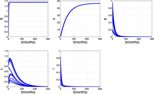From this figure, we can see that there are always susceptible and vaccinated in the population while the infected individuals disappear. Thus the trajectories converge to the DFE. This mean that disease disappears in the host population as shown in Theorem 3.1.Figure 4 gives the trajectory plot when $\lambda =10$, $\beta =0.005$, $\epsilon =0.65$ so that ${\mathcal{R}}_0>1$. From this figure, we can see that whatever the initial point, the infected individuals (Earlier latent, TB infectious and Later latent) remain in the population and stabilize in time. This means that the trajectories converge to the endemic equilibrium point. Thus, as established in Theorem 4.2, the disease persists in the host population whenever ${\mathcal{R}}_0>1$.

Figure 3. Simulation results showing the global stability of the DFE.

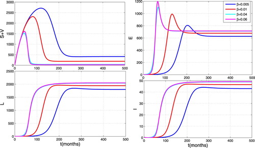
5.2. Impact of the effective contact rate

In order to investigate the impact of the effective contact rate on the propagation of TB, we carry out some numerical simulations to show the contribution of effective contact rate during the whole infection. We set the contact rate β as 0.005, 0.01, 0.04 and $\beta =0.06$. From Figure 5, we can observe that infected individuals reach a higher peak level as β increases. This figure illustrates the great influence of the effective contact rate as shown in the sensitivity analysis.

Figure 4. Simulation results showing the global stability of endemic equilibrium.

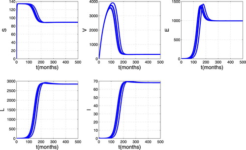
Figure 5. Impact of effective contact rate on the spread of TB.

5.3. Impact of vaccine coverage

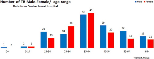
To study the impact of the TB control strategy by vaccination, we carry out simulations by varying vaccine coverage ϵ. We set the vaccine coverage as 0.1, 0.5, 0.9. We can see from Figure 6 that the TB trajectory below all others is the one with the highest vaccination coverage $\epsilon =0.9$. Therefore, high vaccine coverage reduces the spread, but does not lead to the eradication of the disease. Thus the strategy of controlling TB by vaccination is still to be optimized in terms of vaccinating in the very early ages of individual to tackle the first peak of infectious at the age of 15 years old to cope with the Jamot Centre hospital results shown in Figure 8.

Figure 6. Impact of vaccination on the spread of TB.

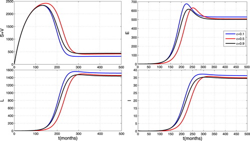
Figure 7 illustrates the impact of a combined effect of contact rate and vaccination coverage rate. One can observe that these combined effects allow to reduce the size of infected individuals. Thus a simultaneous increase of the effectiveness vaccination rate, vaccination coverage rate and the quarantining of infected individuals is an effective control measure against TB infection.

Figure 7. Impact of contact rate and vaccination coverage rate on the spread of TB.

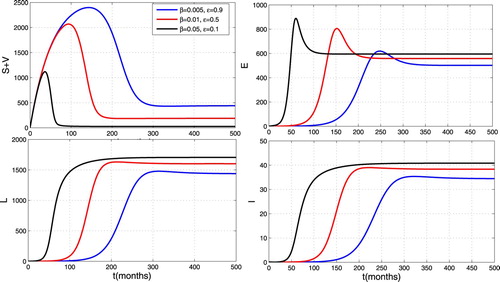
Figure 8. M/F age TB distribution.

6. Conclusion and discussion

The aim of this paper was to extend a basic model without control of TB propagation (S E L I) (Susceptible, Early Latent, Late Latent, Infectious TB) to a model with vaccination as a control strategy. We investigated the effects of the effective contact and vaccination rate on the spread of the TB infection. Using the next generation operator approach, we have derived an explicit formula for the basic reproduction number, ${\mathcal{R}}_0$, which has been the key parameter in our model. Important parameters in the expression of ${\mathcal{R}}_0$ are the contact rate, the recruitment rate and the efficacy of the vaccine. Using the method of global Lyapunov functions, we have established the global stability results of equilibrium points. Precisely, we have shown that the DFE is globally asymptotically stable if ${\mathcal{R}}_0<1$ and unstable otherwise. For the case where ${\mathcal{R}}_0>1$, we have proven that there exists a unique endemic equilibrium, which is globally asymptotically stable. Some numerical simulations are conducted to illustrate that the infection disappears of the population with time when ${\mathcal{R}}_0$ is less than the unity (see Figure 3) but persists in the population when ${\mathcal{R}}_0$ is great than unity (see Figure 5).

In terms of controlling the spread of TB by vaccination, we show that although vaccination reduces the spread, it does not completely eradicate TB in the community when the effective contact rate is high (i.e. cities, jails), until the vaccine remains imperfect (efficacy of TB vaccine is around 50$\mathrm{\%}$) and the policy of vaccination not optimized in terms of vaccinating in the very early ages of individual to tackle the first peak of infectious at the age of 15 as shown in Figure 8. To deeply have a great impact in the limitation of TB spreading, we must act on some key parameters in order to reduce influence of effective contact rate. The control of the spread of HIV/AIDS, the reducing of poverty, the improvement of living conditions in prisons, the sensitization of the populations, the optimization of the strategy of vaccination focussed in the early ages to tackle or prevent efficiently the first peak at the very early ages.

Acknowledgments

The first author acknowledges with thanks, The Chair of Computational Mathematics at DeustoTech Laboratory in the University of Deusto, Bilbao (Basque Country, Spain), the Center for Tuberculosis Screening and Treatment Jamot Hospital, Yaounde-Cameroon.

Disclosure statement

No potential conflict of interest was reported by the authors.

ORCID

Leontine Nkague Nkamba  https://orcid.org/0000-0001-8333-4118

Additional information

Funding

This work was supported by Women for Africa Foundation in collaboration with Diputacion Foral de Bizkaia and Deustotech-Deusto Foundation.

References

- E. Beretta and Y. Takeuchi, Global asymptotic stability of Lotka–Volterra diffusion models with continuous time delay, SIAM J. Appl. Math. 48(3) (1988), pp. 627–651. doi: 10.1137/0148035
- T. Berge, S. Bowong, J. Lubuma, and M.L.M. Manyombe, Modeling Ebola virus disease transmissions with reservoir in a complex virus life ecology, Math. Biosci. Eng. 15(1) (2018), pp. 21–56. doi: 10.3934/mbe.2018002
- S.M. Blower, A.R. McLean, T.C. Porco, P.M. Small, P.C. Hopwell, M.A. Sanchez, and A.R. Ross, The intrinsic transmission dynamics of tuberculosis epidemics, nature medicine, Histoire de l'Acad. Roy. Sci. (Paris) avec Mém. des Math. et Phys. and Mé.
- T.F. Brewer, S.J. Heymann, A.A. Colditz, M.E. Wilson, K. Auerbach, D. Kane, and H.V. Fineberg, Evaluation of tuberculosis control policies using computer simulation, JAMA 276(23) (1996), pp. 1898–1903. doi: 10.1001/jama.1996.03540230048034
- Centers for Disease Control and Prevention (CDC) and others, The Pink Book: Epidemiology and Prevention of Vaccine Preventable Diseases, 10th ed.
- G.A. Colditz, T.F. Brewer, C.S. Berkey, M.E. Wilson, E. Burdick, H.V. Fineberg, and F. Mosteller, Efficacy of BCG vaccine in the prevention of tuberculosis: Meta-analysis of the published literature, JAMA 271(9) (1994), pp. 698–702. doi: 10.1001/jama.1994.03510330076038
- O. Diekmann, J.A.P. Heesterbeek, Mathematical Epidemiology of Infectious Diseases: Model Building, Analysis and Interpretation, Vol. 5, John Wiley & Sons, west sussex, 2000.
- R. Diel, D. Goletti, G. Ferrara, G. Bothamley, D. Cirillo, B. Kampmann, C. Lange, M. Losi, R. Markova, G.B. Migliori, A. Nienhaus, M. Ruhwald, D. Wagner, J.P. Zellweger, E. Huitric, A. Sandgren, and D. Manissero, Interferon-gamma release assays for the diagnosis of latent mycobacterium tuberculosis infection: A systematic review and meta-analysis, Eur. Respir. J. 37 (2011), pp. 88–99. doi: 10.1183/09031936.00115110
- H. Guo and M.Y. Li, Global stability in a mathematical model of tuberculosis, Canad. Appl. Math. Quart. 14 (2006), pp. 185–197.
- J.M. Hyman and J. Li, Differential susceptibility epidemic models, J. Math. Biol. 50(6) (2005), pp. 626–644. doi: 10.1007/s00285-004-0301-7
- M.L.M. Manyombe, J. Mbang, J. Lubuma, and B. Tsanou, Global dynamics of a vaccination model for infectious diseases with asymptomatic carriers, Math. Biosci. Eng. 13(4) (2016), pp. 813–840. doi: 10.3934/mbe.2016019
- S. Marino, I.B. Hogue, C.J. Ray, and D.E. Kirschner, A methodology for performing global uncertainty and sensitivity analysis in systems biology, J. Theor. Biol. 254 (2008), pp. 178–196. doi: 10.1016/j.jtbi.2008.04.011
- D.P. Moualeu, S. Bowong, J. Kurths, Parameter estimation of a tuberculosismodel in a patch environment: Case of Cameroon, Proc. Int. Sym. Math. Comput. Biol. 5 (2013), pp. 352–373.
- J.P. Narain, M.C. Raviglione, and A. Kochi, HIV-associated tuberculosis in developing countries: Epidemiology and strategies for prevention, Tuber. Lung Dis. 73(6) (1992), pp. 311–321. doi: 10.1016/0962-8479(92)90033-G
- National Institute of Statistics, Evolution des systèmes statistiques nationaux – Cameron, 2007.
- National Institute of Statistics, Rapport sur la présentation des résultats définitifs. Technical report, Bureau Central des Recensements et des Etudes de Population, 2010.
- A.J. Rubel and L.C. Garro, Social and cultural factors in the successful control of tuberculosis, Public Health Rep. 107(6) (1992), p. 626.
- R.W. West and J.R. Thompson, Modeling the impact of HIV on the spread of tuberculosis in the united states, Math. Biosci. 143(1) (1997), pp. 35–60. doi: 10.1016/S0025-5564(97)00001-1
- World Health Organization, Media centre: Poliomyelitis, fact sheet, Updated April 2016. Available at http://www.who.int/mediacentre/factsheets/fs114/en/#.
- World Health Organization et al., Global Tuberculosis Report, 2016.