Local approximation of Markov chains in time and space

ABSTRACT

In epidemic modelling, the emergence of a disease is characterized by the low numbers of infectious individuals. Environmental randomness impacts outcomes such as the outbreak or extinction of the disease in this case. This randomness can be accounted for by modelling the system as a continuous time Markov chain, $X\left(t\right)$. The probability of extinction given some initial state is the probability of hitting a subset of the state space associated with extinction for the initial state. This hitting probability can be studied by passing to the discrete time Markov chain (DTMC), $X_n$. An approach is presented to approximate a DTMC on a countably infinite state space by a DTMC on a finite state space for the purpose of solving general hitting problems. This approach is applied to approximate the probability of disease extinction in an epidemic model. It is also applied to evaluate a heterogeneous disease control strategy in a metapopulation.

KEYWORDS:

• Epidemiology
• population dynamics
• public health
• Markov chain

1. Introduction

Early mathematical models of disease considered infection in a single population compartmentalized into susceptible and infectious classes [34,44]. Such models continue to be of interest to researchers to this day [2,10,13,24,32,36,37]. In recent years, increases in mobility, or the processes by which individuals change their location, has motivated researchers to adapt models to consider the spatio-temporal spread of disease [7]. One technique to capture spatial heterogeneity is called metapopulation modelling [6,8,31]. In these models, the population is broken down into subpopulations called patches. Individuals experience patch-specific local interactions as well as migration between patches. Patches are often considered to be separate spatial locations [8]. Deterministic metapopulation models of the spread of infectious disease are often concerned with the asymptotic behaviour of solutions in a neighbourhood of the disease-free equilibrium and those in a neighbourhood of an endemic equilibrium [4,5,8,9,27]. Another important topic for analysis is the question of persistence or extinction of the disease. In deterministic models, the basic reproduction number [19,45] is often used to formulate a sharp threshold for the persistence of the disease [18,23,28,39,47].

When considering the case of the emergence or reemergence of the disease, it becomes necessary to account for the effects of random fluctuations on the dynamics of the system. One technique to account for this stochasticity is to formulate a continuous time Markov chain (CTMC) model. In this setting, random fluctuations will always ultimately lead to the extinction of the disease. Keeling describes a stochastic population as persistent if extinction events are rare [31]. This can be measured by calculating the mean extinction time and comparing it to ecological time scales [30–32] or by calculating the probability of extinction. The probability of extinction is often impossible to calculate directly from the Markov chain, but it can sometimes be approximated by the extinction of a branching process [3,12,37,38]. In the case of a single infectious type, a branching process model takes the form of the classical Galton-Watson branching process (GWbp) [3,48,51]. In the case of multiple infectious types, the branching process takes the form of a multitype branching process [3,26,37,38]. Whether there is a single infectious type or multiple, we will generally refer to approximation via branching process techniques as the branching process approximation. However, the branching process approximation is not appropriate in all cases [38]. In any case, the probability of extinction is the probability of hitting the subset of the state space associated with the extinction of the disease.

CTMC models of biological processes typically assume that the time until the next transition is exponentially distributed. In this case, the hitting problem can be studied by first passing to the embedded discrete time Markov chain (DTMC). In this article, we present an approach to approximate the general hitting problem in a discrete time Markov chain called local approximation in time and space (LATS). We prove that the hitting probability calculated using LATS converges asymptotically to the true hitting probability in Section 3.3. We illustrate this approach via applications in Sections 4 and 5. There are ulterior motives for the choices of applications in Sections 4 and 5. In addition to providing an example of two ways in which the LATS technique provides an approximation of the probability of extinction, the application in Section 4 illustrates that LATS approximation is accurate at small population sizes (when branching process approximations fail) and that LATS provides insight into the most likely path to extinction or outbreak. In Section 5, the LATS technique is used to calculate an atypical hitting problem, illustrating its robustness as a method for approximating general, rather than specific hitting problems.

Stochastic Susceptible-Infected-Susceptible (SIS) models have been a topic of study dating back to the work of Bailey [11]. While some authors have modelled stochasticity using stochastic differential equations [24], we will focus on SIS models in the form of Markov processes. West and Thompson [50] analysed continuous and discrete time SI models and Allen and Burgin [2] compared deterministic and stochastic SIS models. Epidemiological models in the form of stochastic SIS models in metapopulations have been studied in various ways [5,10]. In particular, several authors have considered optimal control [13,35,36]. To illustrate the utility and robustness of the LATS technique, we will formulate the optimal control problem as a hitting problem and analyse it using LATS.

In contrast with branching process approximation, the LATS approach can be used to answer any question about a stochastic metapopulation that can be posed as a hitting problem. For example, the probability of extinction in a single patch may provide important information about a metapopulation. Since patches in a metapopulation are typically coupled together by the migration of their residents, extinction in one patch is a transient event. However, the probability of extinction in a single patch can be used as a patch-specific indicator of disease risk. To illustrate this, we consider a two-patch SIS model in which disease control that reduces the rate of infection by 20% can only be deployed in a single patch. The probability of extinction in a single patch is used to determine the optimal strategy for deployment. We also calculate the optimal strategy using various standard techniques, for comparison.

The article is organized as follows: we begin by recalling the necessary mathematical preliminaries in Section 2. The LATS approach is presented in Section 3. Section 4 illustrates an application of LATS to calculate the probability of the extinction of the disease in a single population where branching process techniques are not suitable. In Section 5, we formulate an optimal control problem in a metapopulation SIS model as a hitting problem to show that analysis via the LATS technique is perhaps more sensitive to the preferences of decision-makers than standard techniques such as the probability of total extinction and ${\mathcal{R}}_0$.

2. Mathematical background and preliminaries

The LATS technique, which is presented in Section 3, combines basic results from the theory of Markov chains, including collapsed Markov chains, and graph theory to formulate an approximation of a given CTMC. For applications to epidemic models, we will typically be concerned with CTMCs which have exponentially distributed waiting times. However, LATS can be applied more generally. In this section, we first recall existing definitions and results pertinent to the development of LATS. A more thorough introduction to the theory of Markov chains can be found in [1,20,22,29,33,40,41].

2.1. Embedded Markov chain

Let $(X_t{)}_{t\ge 0}$ be a homogeneous CTMC on a countable state space S. We ignore the special case of an explosive process [1,40]. Let $(W_i{)}_{i\in \mathbb{N}}$ be the collection of random jump times such that $X_t$ jumps to a new state at each time $W_i$ and remains in the state $X_{W_i}$ for $W_i\le t<W_{i+1}$. The random variables $T_i=W_{i+1}-W_i$ represent the random amount of time $X_t$ spends in state $X_{W_i}$ for each i and are called interevent times. The CTMC $X_t$ can be characterized by its transition probabilities $p_{ij}\left(\mathrm{\Delta }t\right)=P(X_{t+\mathrm{\Delta }t}=j|X_t=i)$ for transition from state i to state j in S. The collection of all transition probabilities can be written as a (possibly infinite) matrix $P\left(t\right)=\left(p_{ij}\right(t\left)\right)$. If $i\ne j$, then $p_{ij}\left(0\right)=0$, otherwise $p_{ii}\left(0\right)=1$. For $i\ne j$, define $q_{ij}=\underset{\mathrm{\Delta }t\to 0^{+}}{lim}\frac{p_{ij}\left(\mathrm{\Delta }t\right)-p_{ij}\left(0\right)}{\mathrm{\Delta }t}=\underset{\mathrm{\Delta }t\to 0^{+}}{lim}\frac{p_{ij}\left(\mathrm{\Delta }t\right)}{\mathrm{\Delta }t}.$ Let $q_{ii}=-\sum _{j\ne i\in S}{q}_{ij}$ and define the generator matrix $Q=\left(q_{ij}\right)$. Let $q_i=-q_{ii}=\sum _{j\ne i\in S}{q}_{ij}$ be the off diagonal ith row sum of Q. The CTMC $X_t$ admits a DTMC $Y_n$, known as the embedded Markov chain. $Y_n$ has the property that $Y_n=X_{W_n},,=0,1,2,\dots .$ Define (1) $t_{ii}=\{\begin{array}{ll}0,& \mathrm{if}{q}_{ii}\ne 0\\ 1,& \mathrm{if}{q}_{ii}=0,\end{array}$(1) and for $j\ne i$ (2) $t_{ij}=\{\begin{array}{ll}\frac{q_{ij}}{q_i},& \mathrm{if}{q}_{ij}\ne 0\\ 0,& \mathrm{if}{q}_{ij}=0.\end{array}$(2) Then the matrix $T=\left(t_{ij}\right)$ is the probability transition matrix of the embedded DTMC $Y_n$. It is equivalent to say that $Y_n$ is formed by conditioning $X_t$ on the fact that a transition has taken place and replacing the index of time with the index of the number of transitions. Since we restrict our discussion to homogeneous CTMCs on a countable state space, any CTMC we consider admits an embedded DTMC. The notation $Y_n$ and T to denote the embedded CTMC and its probability transition matrix can be found in [1] and is used to differentiate between the CTMC and its embedded chain, but is not the standard notation for a DTMC. For the discussions that follow we adopt the following more standard notation for DTMCs.

Let $X_n$ be a homogeneous discrete time Markov chain on a countable state space S. Let P be the probability transition matrix associated with $X_n$. For $i,j\in S$ the one-step transition probability from i to j is given by $p_{ij}=P(X_{n+1}=j|X_n=i).$ The m-step transition probability from i to j is given by $p_{ij}^{\left(m\right)}=P(X_{n+m}=j|X_n=i).$ Since $X_n$ is a homogeneous DTMC, $p_{ij}$ and $p_{ij}^{\left(m\right)}$ are independent of n. Then $(P{)}_{ij}=p_{ij}$ and $(P^m{)}_{ij}=p_{ij}^{\left(m\right)}$. If there is an m>0 such that $p_{ij}^{\left(m\right)}>0$, then we say that j is reachable from i. If j is reachable from i and i is reachable from j, we say that i and j communicate. Communication is an equivalence relation which partitions S into equivalence classes called communication classes. We say a communication class C is closed if whenever $i\in C$ and j is reachable from i, then $j\in C$. A state which is in a communication class which is not closed is called a transient state. The probability of first reaching state j from state i in with respect to $X_n$ is called a hitting probability. The following definitions of the m-step hitting probability and hitting probability come from Pinsky and Karlin [41], while the notation is more similar to that of Norris [40], but modified to suit our purposes. The probability of first hitting state j from state i in exactly m transitions with respect to $X_n$ is an m-step hitting probability and given by (3) $h_{(i;X)}^{\left(m\right)}\left(j\right)=P(X_m=j|X_0=i\cap X_k\ne j\mathrm{\forall }k=1,\dots ,m-1).$(3) The probability of first hitting j from i with respect to $X_n$ is (4) $h_{(i;X)}\left(j\right)=\sum _{m=0}^{\mathrm{\infty }}{h}_{(i;X)}^{\left(m\right)}\left(j\right)=\underset{N\to \mathrm{\infty }}{lim}\sum _{m=0}^N{h}_{(i;X)}^{\left(m\right)}\left(j\right).$(4)

2.2. Graph theory

We now recall a few notions from graph theory [14,15,49]. A graph $\mathfrak{G}$ is a set of vertices $V\left(\mathfrak{G}\right)$ together with a set of edges $E\left(\mathfrak{G}\right)$. The graph $\mathfrak{G}$ is called a directed graph or a di-graph if $E\left(\mathfrak{G}\right)$ is a set of ordered pairs such that $(u,v)\in E\left(\mathfrak{G}\right)$ whenever there is a directed edge from vertices u to v. We say that u is the tail and v is the head of edge $(u,v)$. The out-degree of a vertex v is the number of edges with tail v. The out-degree of the graph $\mathfrak{G}$ is the supremum of the out-degrees taken over all the vertices. For our purposes, we will consider the case that $V\left(\mathfrak{G}\right)$ is a countable set. In this case, $V\left(\mathfrak{G}\right)$ can be enumerated as a sequence $\left(v_i\right)$ for $i=1,2,3,\dots$. Define the (possibly infinite) matrix $A=\left(a_{ij}\right)$ with entry $a_{ij}=1$ if $(v_i,v_j)\in E\left(\mathfrak{G}\right)$ and $a_{ij}=0$ otherwise. The matrix A is called the adjacency matrix of the graph $\mathfrak{G}$. Clearly, A encodes the edge set $E\left(\mathfrak{G}\right)$. If the vertex set $V\left(\mathfrak{G}\right)$ is understood, then A defines the graph $\mathfrak{G}$. A u,v-path of length k is a sequence $v_{i_0},e_1,v_{i_1},e_2,\dots ,e_k,v_{i_k}$ where $v_{i_0}=u$, $v_{i_k}=v$ and $e_j=(v_{i_{j-1}},v_{i_j})$ for $j=1,2,\dots ,k$. The graph distance between vertices u and v, denoted $\mathfrak{d}(u,v)$, is defined as the length of the shortest u,v-path. We take the convention that $\mathfrak{d}(u,v)=0$ if u=v and $\mathfrak{d}(u,v)=\mathrm{\infty }$ if there is no path from u to v. Since $\mathfrak{G}$ is a directed graph, the graph distance is typically a quasi-metric (i.e. it meets all the conditions of a metric except symmetry). The ball of radius r in the graph $\mathfrak{G}$ centred at the vertex v, denoted $B(v,r)$, is the subset of vertices u such that $\mathfrak{d}(v,u)\le r$.

Let us return our attention to the DTMC $X_n$ on the countable state space S with probability transition matrix $P=\left(p_{ij}\right)$. Let A be the adjacency matrix induced by P such that (5) ${\left(A\right)}_{ij}=a_{ij}=\{\begin{array}{ll}1& \mathrm{if}{p}_{ij}>0,\\ 0& \mathrm{if}{p}_{ij}=0.\end{array}$(5) In this way, $X_n$ induces a di-graph, $\mathfrak{G}$, with states in the state space S as vertices. By the definition of A given in (5(5) ${\left(A\right)}_{ij}=a_{ij}=\{\begin{array}{ll}1& \mathrm{if}{p}_{ij}>0,\\ 0& \mathrm{if}{p}_{ij}=0.\end{array}$(5) ), if there is a positive probability of transitioning from i to j in $X_n$, then there is an edge $(i,j)$ in $\mathfrak{G}$. Therefore, if $p_{ij}^{\left(m\right)}>0$, then there is a, i,j-path in $\mathfrak{G}$ of length m. It follows that the distance in the induced graph is given by $\mathfrak{d}(i,j)=inf\{m\ge 0|p_{ij}^{\left(m\right)}>0\}$. In addition, the ball of radius r in the induced graph centred at i is $B(i,r)=\{j|p_{ij}^{\left(m\right)}>0\mathrm{for}\mathrm{some}m\le r\}$.

2.3. Finite absorbing Markov chains

Now let $X_n$ be a homogeneous DTMC on a finite state space S with the properties that there is at least one closed communication class, there is at least one communication class which is not closed and that all closed communication classes are singletons. This makes $X_n$ an absorbing Markov chain. The closed communication classes of an absorbing Markov chain are called absorbing states. A more complete discussion of finite absorbing Markov chains can be found in Chapter 3 of [33]. Let P be the probability transition matrix of $X_n$. Suppose that $|S|=m$ and S contains j<m absorbing states. By simultaneously exchanging rows and columns of P, we can put it in its canonical form (6) $P=\left[\begin{array}{cc}I& 0\\ \left[2pt/2pt\right]C& D\end{array}\right],$(6) where I is the $j\times j$-identity matrix and D is the substochastic $m-j\times m-j$ matrix. The matrix $(I-D{)}^{-1}$ is called the fundamental matrix of $X_n$.

Theorem 2.1

[33]

Let $X_n$ be a homogeneous DTMC on the state space S with $|S|=m$. Let the probability transition matrix of $X_n$ be given by (6(6) $P=\left[\begin{array}{cc}I& 0\\ \left[2pt/2pt\right]C& D\end{array}\right],$(6) ). Then $\underset{n\to \mathrm{\infty }}{lim}{P}^n=\left[\begin{array}{cc}I& 0\\ \left[2pt/2pt\right]H& 0\end{array}\right],$ where $H=(I-D{)}^{-1}C$. Furthermore, for $i=j+1,\dots ,m$ and $k=1,\dots ,j$, the entry, $H_{ik}$, associated with i and k is the probability of hitting the absorbing state $s_k$ from the transient state $s_i$, $h_{(s_i;X)}\left(s_k\right)$.

2.4. Collapsed chains

We now return to our discussion of the homogeneous DTMC $X_n$ on the countable state space S with probability transition matrix P. Following Hachigian [25], consider the collapsed process $Y_n=f\left(X_n\right)$ where f is a many-to-one function on S onto the state space of $Y_n$. Suppose that the states of $Y_n$ are denoted by the countable sequence $(S_{\alpha }{)}_{\alpha \in I}$. For each α in the index set I, we say that the subset of states i of S given by $f^{-1}\left(S_{\alpha }\right)$ are collapsed into the single state $S_{\alpha }$ of the process $Y_n$. It is not generally the case that the process $Y_n$ possesses the Markov property. It is natural to ask under what conditions the process resulting from collapsing a Markov process is again Markov. Several researchers have made contributions to this field [16,17,25,42,43]. The following result gives a sufficient condition in the case $X_n$ is a finite state space Markov chain. The result is given for non-homogeneous chains.

Theorem 2.2

[17]

Let $X_n$, $n\ge 0$, be a non-homogeneous Markov chain with any given initial distribution vector p and the state space $S=\{1,2,\dots ,m\}$. Let $1\le r\le m$, and $S_1,S_2,\dots ,S_r$ be r pairwise disjoint subsets of $S=\bigcup _{i=1}^r{S}_i$. Let $Y_n$, $n\ge 0$, be the collapsed chain defined by $Y_n=i$ if and only if $X_n\in S_i$. Then a sufficient condition for $Y_n$ to be Markov is that $P(X_n\in S_j|X_{n-1}=k)$ is independent of k in $S_i$ for $1\le i\le r,1\le j\le r,i\ne j,n\ge 2$.

3. Local approximation in time and space

In this section, we present a technique called LATS for studying certain features of homogeneous DTMCs or homogeneous CTMCs by first passing to the embedded DTMC. As such, the details will be presented in terms of a DTMC $X_n$ on a countable state space S with probability transition matrix P. In broad strokes, LATS consists of first restricting to a subset of the state space S, modifying this subset to form a state space $\mathcal{S}$ so that $X_n$ induces a DTMC $Z_n$ on $\mathcal{S}$. We will show that $Z_n$ faithfully approximates $X_n$ locally in time and space. We then collapse $Z_n$ on $\mathcal{S}$ to an absorbing DTMC $Y_n$ on the collapsed state space $\mathcal{S}$. Analysis of the collapsed chain $Y_n$ is more straightforward and less computationally expensive.

3.1. Neighbourhood of a set of states

The first step in the LATS technique is to form a subset of a set the state space S. Let $T\subset S$. For any $m\ge 0$ define $p_{Tj}^{\left(m\right)}:=\sum _{i\in T}{p}_{ij}^{\left(m\right)}$.

Definition 3.1

Let $X_n$ be a homogeneous DTMC on a countable state space S. Let $T\subset S$ and $N\in \mathbb{N}$. The N-neighbourhood of the set T with respect to $X_n$ is defined as (7) ${\mathcal{N}}_N\left(T\right)=\{s\in S:\mathrm{\exists }m\le N\mathrm{such}\mathrm{that}{p}_{Ts}^{\left(m\right)}>0\}=\bigcup _{s\in T}B(s,N),$(7) where $B(s,N)$ is the ball of radius N centred at s in the graph $\mathfrak{G}$ induced by $X_n$ as described in Section 2.2.

Note that ${\mathcal{N}}_0\left(T\right)=T$, since $p_{ii}^{\left(0\right)}=1$ by convention. Let $R_N\left(T\right)$ be the submatrix of the probability transition matrix P associated with the states in ${\mathcal{N}}_N\left(T\right)$. If T is a proper subset of S, then R is typically a substochastic matrix. In order to extend $R_N$ to a stochastic matrix, we must extend the N-neighbourhood by adding an additional absorbing state. Let ${\delta }_i\left(j\right)$ be the Dirac delta function with ${\delta }_i\left(j\right)=1$ when i=j and zero otherwise.

Definition 3.2

By the state space associated with ${\mathcal{N}}_N\left(T\right),$ we mean ${\mathcal{S}}_N\left(T\right)={\mathcal{N}}_N\left(T\right)\cup \left\{g\right\}$, where g is a new state associated with escape from ${\mathcal{N}}_N\left(T\right)$. Define the transition matrix $Q_N\left(T\right)$ on ${\mathcal{S}}_N\left(T\right)$ by (8) $Q_N\left(T\right):=\{\begin{array}{ll}{q}_{ij}=p_{ij}& \mathrm{for}i,j\in {\mathcal{N}}_N\left(T\right)\\ q_{ig}=1-\sum _{j\in {\mathcal{N}}_N\left(T\right)}{p}_{ij}& \mathrm{for}i\in {\mathcal{N}}_N\left(T\right)\\ q_{gi}={\delta }_g\left(i\right).\end{array}$(8) $Q_N\left(T\right)$ is a stochastic matrix which can be written (9) $Q_N\left(T\right)=\left[\begin{array}{cccccc}& & & & & ⋮\\ & & R_N\left(T\right)& & & q_{ig}\\ & & & & & ⋮\\ \left[2pt/2pt\right]& \cdots & 0& \cdots & & 1\end{array}\right].$(9)

Since $Q_N\left(T\right)$ is stochastic, it induces a DTMC, $Z_n$, on the state space ${\mathcal{S}}_N\left(T\right)$. If the out-degree of the graph and the set of initial states T are both finite, then the state space ${\mathcal{S}}_N\left(T\right)$ is finite. The next result shows that for any initial distribution supported on states in T, $Z_n$ approximates $X_n$ locally in time.

Theorem 3.1

Let $P=\left(p_{ij}\right)$ be the probability transition matrix of the DTMC $X_n$ on the countable state space S, let $T\subset S$ and $N\ge 1$. Suppose that ${\mathcal{N}}_N\left(T\right)$ and $Q_N\left(T\right)=\left(q_{ij}\right)$ are as defined in (7(7) ${\mathcal{N}}_N\left(T\right)=\{s\in S:\mathrm{\exists }m\le N\mathrm{such}\mathrm{that}{p}_{Ts}^{\left(m\right)}>0\}=\bigcup _{s\in T}B(s,N),$(7) ) and (8(8) $Q_N\left(T\right):=\{\begin{array}{ll}{q}_{ij}=p_{ij}& \mathrm{for}i,j\in {\mathcal{N}}_N\left(T\right)\\ q_{ig}=1-\sum _{j\in {\mathcal{N}}_N\left(T\right)}{p}_{ij}& \mathrm{for}i\in {\mathcal{N}}_N\left(T\right)\\ q_{gi}={\delta }_g\left(i\right).\end{array}$(8) ) above. For $x\in T$, $\sum _{i\in {\mathcal{N}}_N\left(T\right)}{q}_{xi}^{\left(m\right)}=\sum _{i\in S}{p}_{xi}^{\left(m\right)}=\sum _{i\in {\mathcal{N}}_N\left(T\right)}{p}_{xi}^{\left(m\right)}=1$ for all $m\le N$.

Proof.

Let $m\le N$. By definition, for $i\in S$, $p_{xi}^{\left(m\right)}=P(X_m=i|X_0=x)$. By the Chapman–Kolmogorov equation, for $0\le n\le m$ $p_{xi}^{\left(m\right)}=\sum _{k\in S}{p}_{xk}^{\left(n\right)}{p}_{ki}^{(m-n)}=\sum _{k_1,\dots ,k_{m-1}\in S}{p}_{x{k}_1}{p}_{k_1{k}_2}\dots p_{k_{m-1}i}.$ Suppose that $k_1,\dots ,k_{m-1}$ are states in S such that $p_{x{k}_1}{p}_{k_1{k}_2}\dots p_{k_{m-1}i}>0$. Then $(x,e_1,k_1,\dots ,k_{m-1},e_m,i)$ is a path of length m from x to i in the induced graph $\mathfrak{G}$. By definition, $k_1,k_2,\dots ,k_{m-1},i\in {\mathcal{N}}_N\left(T\right)$. It follows that $p_{x{k}_1}{p}_{k_1{k}_2}\dots p_{k_{m-1}i}=q_{x{k}_1}{q}_{k_1{k}_2}\dots q_{k_{m-1}i}$. Therefore, $\begin{array}{rl}{p}_{xi}^{\left(m\right)}& =\sum _{k_1,\dots ,k_{m-1}\in S}{p}_{x{k}_1}{p}_{k_1{k}_2}\dots p_{k_{m-1}i}=\sum _{k_1,\dots ,k_{m-1}\in {\mathcal{N}}_N\left(T\right)}{p}_{x{k}_1}{p}_{k_1{k}_2}\dots p_{k_{m-1}i}\\ & =\sum _{k_1,\dots ,k_{m-1}\in {\mathcal{N}}_N\left(T\right)}{q}_{x{k}_1}{q}_{k_1{k}_2}\dots q_{k_{m-1}j}=q_{xi}^{\left(m\right)}.\end{array}$

Let π be any initial distribution on S. Let $\text{ supp }\left(\pi \right)$ be the support of π. If $\text{ supp }\left(\pi \right)\subset T$, then there is a distribution on $\mathcal{S}$, say $\stackrel{\sim }{\pi }$, which is supported on $\text{ supp }\left(\pi \right)$ and equal to π there. Theorem 3.1 shows that the evolution of the distribution π in the chain $X_n$ is completely captured by the evolution of the distribution $\stackrel{\sim }{\pi }$ in the chain $Z_n$ for the first N transitions.

3.2. Collapsing $Z_n$

The definition of ${\mathcal{S}}_N\left(T\right)$ is related to the graph $\mathfrak{G}$ induced by the underlying Markov chain $X_n$ by (7(7) ${\mathcal{N}}_N\left(T\right)=\{s\in S:\mathrm{\exists }m\le N\mathrm{such}\mathrm{that}{p}_{Ts}^{\left(m\right)}>0\}=\bigcup _{s\in T}B(s,N),$(7) ). If the set of initial states T and the out-degree of $\mathfrak{G}$ are both finite, then ${\mathcal{S}}_N\left(T\right)$ is finite for each N. Nevertheless, $|{\mathcal{S}}_N\left(T\right)|$ may be quite large, making a direct analysis of $Z_n$ difficult. In order to reduce the complexity of the mathematical analysis of $Z_n$, as well as the computational expense for calculations, the next step is to collapse $Z_n$ to an absorbing DTMC $Y_n$. As noted in Section 2.4, $Y_n=f\left(Z_n\right)$ is a collapsed chain for any many-to-one function f from the state space of $Z_n$ to the state space of $Y_n$. However, not all collapsed chains are themselves Markov. We recalled the definition of a closed communication class above. Now we make a more general definition of a closed subset of the state space.

Definition 3.3

Let $X_n$ be a homogeneous DTMC on the finite state space S and let $C\subset S$. We say that C is closed with respect to communication if, whenever $i\in C$ and $j\in S\setminus C$, then $p_{ij}=0$.

As noted above, we seek a function f so that $Y_n=f\left(Z_n\right)$ is an absorbing Markov chain. Absorbing states in a collapsed chain are either the result of the identity map on an absorbing state in the original chain or they are the result of collapsing a subset of the state space which is closed with respect to communication. Theorem 3.2 shows that collapsing a closed set results in a Markov chain.

Theorem 3.2

Let $X_n$ be a homogeneous DTMC on a countable state space S. Let $C\subset S$ be a proper subset of the state space which is closed with respect to communication. Let f be a many-to-one function given by $f\left(s\right)=\{\begin{array}{ll}s& \mathrm{if}s\in S\setminus C,\\ c& \mathrm{if}s\in C.\end{array}$ Then $Y_n=f\left(X_n\right)$ is a Markov chain.

Proof.

Let $x\in S\setminus C$ and $y\in C$. Since C is closed with respect to communication, for all $m\ge 0$ $P(X_m=x|X_0=y)=0$ and $P(X_m\in C|X_0=y)=1.$ Therefore, the closed set C is mapped to an absorbing state c. Let $x_0,\dots ,x_{m-1},x_m\in S\setminus C$. Then $P(Y_m=x_m|Y_0=x_0,\dots ,Y_{m-1}=x_{m-1})=P(Y_m=x_m|Y_{m-1}=x_{m-1})$ is inherited from $X_n$. Furthermore, $\begin{array}{rl}P(& Y_m=c|Y_0=x_0,\dots ,Y_{m-1}=x_{m-1})=\sum _{s\in C}P(X_m=s|X_0=x_0,\dots ,X_{m-1}=x_{m-1})\\ & =\sum _{s\in C}P(X_m=s|X_{m-1}=x_{m-1})=P(X_m\in C|X_{m-1}\\ & =x_{m-1})=P(Y_m=c|Y_{m-1}=x_{m-1}).\end{array}$ Now let $y\in S\setminus C\cup \left\{c\right\}$. Consider (10) $P(Y_m=y|Y_0=x_0,\dots ,Y_{m-2}=x_{m-2},Y_{m-1}=c).$(10) Since $Y_{m-1}=c$, there exists $s\in C$ such that $X_{m-1}=s$. Then $\begin{array}{rl}\left(10\right)& =\{\begin{array}{ll}P(X_m=y|X_0=x_0,\dots ,X_{m-2}=x_{m-2},X_{m-1}=s)& y\in S\setminus C\\ P(X_m\in C|X_0=x_0,\dots ,X_{m-2}=x_{m-2},X_{m-1}=s)& y=c\end{array}\\ & =\{\begin{array}{ll}P(X_m=y|X_{m-1}=s)& y\in S\setminus C\\ \sum _{r\in C}P(X_m=r|X_{m-1}=s)& y=c\end{array}\\ & ={\delta }_c\left(y\right)\\ & =P(Y_m=y|Y_{m-1}=c).\end{array}$

To form the state space ${\mathcal{S}}_N\left(T\right)$ of the chain $Z_n$, we eliminated the complement of the N-neighbourhood ${\mathcal{N}}_N\left(T\right)$ in the state space S and replaced it with an absorbing state g. In light of Theorem 3.2, we see that the escape state g can be formed, for example, by making all states in the complement of ${\mathcal{N}}_N\left(T\right)$ absorbing and collapsing the resulting closed (possibly infinite) set.

Corollary 3.3

Let $X_n$ be a homogeneous DTMC on a countable state space S. Suppose that $S=A\cup \bigcup _{i=1}^{\mathrm{\infty }}{S}_i$ is a decomposition of S into the union of disjoint sets $A,S_1,S_2,\dots$, where $S_i$ is closed with respect to communication for all $i\ge 1$. Let f be a many-to-one map such that $f\left(S_i\right)=i$ for all $i\ge 1$ and $f{|}_A$ is the identity. Then $Y_n=f\left(X_n\right)$ has the Markov property. If $x\in A$ and $i\ge 1$, then $h_{(x;X)}\left(S_i\right)=h_{(x;Y)}\left(i\right),$ where $h_{(x;X)}\left(S_i\right)$ and $h_{(x;Y)}\left(i\right)$ are hitting probabilities as in (4(4) $h_{(i;X)}\left(j\right)=\sum _{m=0}^{\mathrm{\infty }}{h}_{(i;X)}^{\left(m\right)}\left(j\right)=\underset{N\to \mathrm{\infty }}{lim}\sum _{m=0}^N{h}_{(i;X)}^{\left(m\right)}\left(j\right).$(4) ).

To approximate the behaviour of a homogeneous DTMC near a set of initial states $T\subset S$, we first form the DTMC $Z_n$ on a local state space ${\mathcal{S}}_N\left(T\right)$ either by adjoining an absorbing state to the N-neighbourhood, ${\mathcal{N}}_N\left(T\right),$ described by (7(7) ${\mathcal{N}}_N\left(T\right)=\{s\in S:\mathrm{\exists }m\le N\mathrm{such}\mathrm{that}{p}_{Ts}^{\left(m\right)}>0\}=\bigcup _{s\in T}B(s,N),$(7) ) or by making the contrivance that $S\setminus {\mathcal{N}}_N\left(T\right)$ is closed with respect to communication and collapsing it. Theorem 3.1 shows that $Z_n$ approximates the behaviour of $X_n$ for N transitions on the condition that $X_0=Z_0\in T$. If we are not concerned with the behaviour of $X_n$ once it enters a closed communication class, we may further simplify the approximation by forming the collapsed chain $Y_n=f\left(Z_n\right)$, where f identifies closed communication classes with absorbing states and f is the identity map on transient states. In the next section, we show how LATS can be used to answer the question: what is the probability of first hitting a particular subset of the state space from a particular state in the chain $X_n$?

3.3. LATS approximation of hitting probabilities

Let $X_n$ be a homogeneous DTMC on a countable state space S. In this section, we describe how LATS can be used to approximate the general hitting problem with respect to $X_n$. By the general hitting problem, we mean to determine the probability $h_x\left(V\right)=h_{(x;X)}\left(V\right)$ where $x\in S$ and $V\subset S$. If $x\in V\subset S$, then $h_x\left(V\right)=1$ is trivial. However, it is not so trivial if $x\in S\setminus V$. For example, if S is finite but very large or S is countably infinite, then the general hitting problem can be difficult or even impossible to determine from direct analysis of $X_n$.

For $x,y\in S$, the probability of first hitting y from x, given by $h_x\left(y\right)$, can be reformulated in terms of x,y-paths in the induced graph $\mathfrak{G}$. By a path of length m which first hits y from x in the graph $\mathfrak{G}$ we mean an x,y-path of length m, as in Section 2.2, with $v_{i_0}=x$, $v_{i_m}=y$ and $v_{i_k}\ne y$ for $k=1,2,\dots ,m-1$. Let $\left({\ell }_i\right(x,y){)}_{i\in I_m}$ be the family of such paths with index set $I_m$. For $i\in I_m$, let $p_i$ be the probability of path ${\ell }_i$. Then (11) $h_x^{\left(m\right)}\left(y\right)=\sum _{i\in I_m}{p}_i.$(11) Equation (4(4) $h_{(i;X)}\left(j\right)=\sum _{m=0}^{\mathrm{\infty }}{h}_{(i;X)}^{\left(m\right)}\left(j\right)=\underset{N\to \mathrm{\infty }}{lim}\sum _{m=0}^N{h}_{(i;X)}^{\left(m\right)}\left(j\right).$(4) ) implies that $\sum _{m=0}^N{h}_x^{\left(m\right)}\left(y\right)$ is a good approximation of $h_x\left(y\right)=h_{(x;X)}\left(y\right)$ for N sufficiently large. Since ${\mathcal{N}}_N\left(x\right)$ depends on N, so does $Z_n$ and $h_{(x;Z)}\left(y\right)$. For $m\le N$ and $i\in I_m$, the path ${\ell }_i$ is entirely contained in ${\mathcal{N}}_N\left(x\right)$. In particular, $y\in {\mathcal{N}}_N\left(x\right)$ and $\sum _{m=0}^N{h}_{(x;Z)}^{\left(m\right)}\left(y\right)=\sum _{m=0}^N{h}_{(x;X)}^{\left(m\right)}\left(y\right)$. It follows that $h_{(x;Z)}\left(y\right)$ increases to $h_{(x;X)}\left(y\right)$ as N increases to infinity.

In order to describe how to use LATS to approximate the general hitting problem, we make the following assumption.

Assumption 3.1

A1

Suppose that $X_n$ induces a graph $\mathfrak{G}$ with finite out-degree. Suppose that T and V are disjoint, proper subsets of S and the goal is to find the probability $h_{(x;X)}\left(V\right)$ for all $x\in T$. For fixed $N\in \mathbb{N}$, form ${\mathcal{N}}_N\left(T\right)$, ${\mathcal{S}}_N\left(T\right)$ and $Q_N\left(T\right)$. This induces the DTMC $Z_n$ as described in Section 3.1. Since both N and the out-degree of $\mathfrak{G}$ are finite, if T is finite, so is ${\mathcal{S}}_N\left(T\right)$. Now make all states in the set $V\cap {\mathcal{S}}_N\left(T\right)$ absorbing. Then $V\cap {\mathcal{S}}_N\left(T\right)$ is closed with respect to communication. Collapse $V\cap {\mathcal{S}}_N\left(T\right)$ to a single absorbing state, which we denote y. In addition, collapse all remaining closed communication classes of $Z_n$. Denote the collapsed chain $Y_n=f\left(Z_n\right)$, its state space ${\mathcal{S}}_N\left(T\right)$ and its probability transition matrix ${\mathcal{Q}}_N\left(T\right)$.

Given (A1), by Corollary 3.3, $Y_n$ is Markov and $h_{(x;Z)}(V\cap {\mathcal{S}}_N(T\left)\right)=h_{(x;Y)}\left(y\right)$ for all $x\in T$. Since $Z_n$ depends on N, so does $Y_n$.

Proposition 3.4

Assume (A1) and suppose that $x\in T$ such that $h_{(x;X)}\left(V\right)>0$. Then x is a transient state in ${\mathcal{S}}_N\left(T\right)$.

Proof.

Since $h_x\left(V\right)>0$, for some $v\in V$ there is a x,v-path in $\mathfrak{G}$. Either $v\in V\cap {\mathcal{N}}_N\left(T\right)$ or $v\in V\setminus {\mathcal{N}}_N\left(T\right)$. If $v\in V\cap {\mathcal{S}}_N\left(T\right)$, then there is an x,y-path in the graph induced by $Y_n$. Since there is a path from x to y, y is reachable from x. Since y is an absorbing state, the singleton $\left\{y\right\}$ is a closed communication class. Therefore, x is not reachable from y. Hence, x is transient in $Y_n$. If $v\in V\setminus {\mathcal{N}}_N\left(T\right)$, then ${\mathcal{S}}_N\left(T\right)$ can be formed by making all states in $S\setminus {\mathcal{N}}_N\left(T\right)$ absorbing and collapsing $S\setminus {\mathcal{N}}_N\left(T\right)$ to the single absorbing state g. Since $V\setminus {\mathcal{N}}_N\left(T\right)\subset S\setminus {\mathcal{N}}_N\left(T\right)$, there is a path from x to g in the graph induced by $Y_n$. The rest of the proof follows the arguments of the previous case.

Theorem 3.5

Assume (A1). For $x\in T$, if $h_{(x;X)}\left(V\right)=0$, then $h_{(x;Y)}\left(y\right)=0$. If $h_{(x;X)}\left(V\right)>0$, then $h_{(x;X)}\left(V\right)-h_{(x;Y)}\left(y\right)\le h_{(x;Y)}\left(g\right)$ and $h_{(x;X)}\left(V\right)-h_{(x;Y)}\left(y\right)$ is non-increasing as a function of N. If ${\mathcal{N}}_N\left(T\right)$ increases to S with N, then $\underset{N\to \mathrm{\infty }}{lim}{h}_{(x;Y)}\left(g\right)=0$.

Proof.

Let $({\ell }_i{)}_{i\in I_m}$ be the collection of all paths of length m which first hit V from x in the graph induced by $X_n$ and let $p_i$ be the probability of ${\ell }_i$. If all of the vertices that comprise the path ${\ell }_i$ are elements of ${\mathcal{N}}_N\left(T\right)$, we write ${\ell }_i\subset {\mathcal{N}}_N\left(T\right)$. If the vertices of ${\ell }_i$ are not all contained in ${\mathcal{N}}_N\left(T\right)$, we write ${\ell }_i\not\subset {\mathcal{N}}_N\left(T\right)$. By the Law of Total Probability, $h_{(x;X)}\left(V\right)=\sum _{m=1}^{\mathrm{\infty }}\sum _{i\in I_m}(p_i|{\ell }_i\subset {\mathcal{N}}_N(T\left)\right)+\sum _{m=1}^{\mathrm{\infty }}\sum _{i\in I_m}(p_i|{\ell }_i\not\subset {\mathcal{N}}_N(T\left)\right)$. By construction, $\sum _{m=1}^{\mathrm{\infty }}\sum _{i\in I_m}(p_i|{\ell }_i\subset {\mathcal{N}}_N(T\left)\right)=h_{(y;Y)}\left(t\right)$. In the case ${\ell }_i\not\subset {\mathcal{N}}_N\left(T\right)$, there is a vertex of ${\ell }_i$ which is an element of $S\setminus {\mathcal{N}}_N\left(T\right)$. Then ${\ell }_i\not\subset {\mathcal{N}}_N\left(T\right)$ corresponds to an x,g-path in the collapsed chain $Y_n$. Therefore, $\sum _{m=1}^{\mathrm{\infty }}\sum _{i\in I_m}(p_i|{\ell }_i\not\subset {\mathcal{N}}_N(T\left)\right)\le h_{(g;Y)}\left(t\right)$. It follows that $h_{(x;X)}\left(V\right)-h_{(x;Y)}\left(y\right)\le h_{(x;Y)}\left(g\right)$. Since ${\mathcal{N}}_N\left(T\right)$ is non-decreasing in N, $\sum _{m=1}^{\mathrm{\infty }}\sum _{i\in I_m}(p_i|{\ell }_i\subset {\mathcal{N}}_N(T\left)\right)=h_{(x;Y)}\left(y\right)$ is non-decreasing. The final claim follows from the fact that if $\underset{N\to \mathrm{\infty }}{lim}{\mathcal{N}}_N\left(T\right)=S$.

Theorem 3.5 proves that $h_{(x;Y)}\left(y\right)$ approximates $h_{(x;X)}\left(V\right)$ and $h_{(x;Y)}\left(g\right)$ is an upper bound on the error of the approximation. To show that error goes to zero requires the additional assumption that ${\mathcal{N}}_N\left(T\right)$ increase to S as N increases to infinity. This seems like a very strong assumption. However, biological phenomena are typically modelled by generalized birth–death processes, which satisfy this assumption. In these and other cases for which the assumption holds, the proof only shows that the error goes to zero asymptotically. However, we will see that in applications the approximation can be very accurate for N<30.

Corollary 3.6

Assume (A1). For $x\in T$ and $m\le N$ (12) $h_{(x;X)}^{\left(m\right)}\left(V\right)=h_{(x;Y)}^{\left(m\right)}\left(y\right).$(12)

Proof.

Let $({\ell }_i{)}_{i\in I_k}$ be the collection of all paths of length k which first hit V from x in the graph induced by $X_n$. Let $p_i$ be the probability of path ${\ell }_i$. If $m\le N$, then (13) $h_{(x;X)}^{\left(m\right)}\left(V\right)=\sum _{k=1}^m\sum _{i\in I_k}(p_i|{\ell }_i\subset {\mathcal{N}}_N(T\left)\right)=h_{(x;Y)}^{\left(m\right)}\left(y\right).$(13)

Theorem 3.7

Assume (A1). For fixed $N\in \mathbb{N}$, if $|T|<\mathrm{\infty }$, then $Y_n$ is a finite absorbing Markov chain with probability transition matrix ${\mathcal{Q}}_N\left(T\right)$ with canonical form (6(6) $P=\left[\begin{array}{cc}I& 0\\ \left[2pt/2pt\right]C& D\end{array}\right],$(6) ). Furthermore, for $m\le N$ and $x\in T$, $\sum _{k=1}^m{h}_{(x;X)}^{\left(k\right)}\left(V\right)={\left({\mathcal{Q}}_N^m\right(T\left)\right)}_{xy},$ where $\left({\mathcal{Q}}_N^m\right(T){)}_{xy}$ is the entry in the row associated with x and column associated with y in the mth power of the probability transition matrix ${\mathcal{Q}}_N\left(T\right)$. Furthermore, $h_{(x;Y)}\left(y\right)$ is the entry in the row associated with x and column associated with y of $H=(I-D{)}^{-1}C$ as in Theorem 2.1.

Proof.

By (A1), the out-degree of the graph $\mathfrak{G}$, induced by $X_n$, is finite. Let $d\in \mathbb{N}$ be the out-degree of $\mathfrak{G}$. It follows that $|{\mathcal{S}}_N\left(T\right)|\le |T|(dN+1)$. Since $|{\mathcal{S}}_N\left(T\right)|\le |{\mathcal{S}}_N\left(T\right)|$, $Y_n$ is a finite Markov chain. The result of collapsing a set which is closed with respect to communication is an absorbing state. By construction, $Y_n$ consists entirely of absorbing states and transient states and is therefore an absorbing Markov chain. That $h_{(x;Y)}\left(y\right)$ is the entry in the row associated with x and column associated with y of $H=(I-D{)}^{-1}C$ is a direct application of Theorem 2.1 to the finite absorbing Markov chain $Y_n$. From Corollary 3.6 $h_{(x;X)}^{\left(m\right)}\left(V\right)=h_{(x;Y)}^{\left(m\right)}\left(y\right)$, for $m\le N$. Since y is an absorbing state, $\sum _{k=1}^m{h}_{(x;Y)}^{\left(k\right)}\left(y\right)={\left({\mathcal{Q}}_N^m\right(T\left)\right)}_{xy}.$

This is a powerful result for practical applications. Since I−D is a nonsingular M -matrix, to find a hitting probability using the LATS method we can use either of ${\mathcal{Q}}_N^n\left(T\right)$ for sufficiently large n or $(I-D{)}^{-1}C$. We will exhibit the practicality of this technique and the nature of the convergence for a particular DTMC by way of example in the next section.

4. LATS vs. branching process techniques

Infectious Salmon Anemia virus (ISAv) causes Infectious Salmon Anemia (ISA) in a variety of finfish including Atlantic salmon (Salmo salar). ISA causes high mortality [21] and affects all major salmon producing countries [46]. It is an important disease to the salmon culture industry which has caused significant economic losses according to the Global Aquaculture Alliance. Deterministic models of an ISAv outbreak in one and two patches are proposed and analysed in [39]. The one-patch model is given by (14) $\begin{array}{rcl}\stackrel{.}{S}& =& S(\beta -\mu S)-S(\eta I+\rho V),\\ \stackrel{.}{I}& =& S(\eta I+\rho V)-\alpha I,\\ \stackrel{.}{V}& =& -\omega V+\delta I,\end{array}$(14) where S denotes susceptible fish, I denotes infected fish and V denotes free-virus in the environment. Susceptible fish experience logistic population growth with birth and death rates β and μ, respectively. The rates of infection due to contact with infected individuals and contact with free-virus are given by η and ρ, respectively. The rate of mortality of infected fish is given by α and the rate infected fish shed virus particles into the environment is δ. Free-virus denatures and is cleared from the environment at rate ω. By scaling the system, we may eliminate η and ρ. This yields the reduced system (15) $\begin{array}{rcl}\stackrel{.}{S}& =& S(\beta -\mu S)-S(I+V),\\ \stackrel{.}{I}& =& S(I+V)-\alpha I,\\ \stackrel{.}{V}& =& -\omega V+\delta I.\end{array}$(15) The state variable V in the reduced system represents the number of infectious doses of free-virus in the environment.

The basic reproduction number is shown to be a critical parameter with the sharp threshold ${\mathcal{R}}_0=1$ separating persistence of the disease (${\mathcal{R}}_0>1$) and its extinction (${\mathcal{R}}_0\le 0$). The emergence of the disease is characterized by low prevalence of the disease in the environment and few infected individuals. This setting demands the use of stochastic modelling techniques to account for inherent random fluctuations. Continuous time Markov chain companion models are developed and analysed in [38]. The CTMC model of a single patch is given by $X_t=(S_t,I_t,V_t)$ and associated infinitesimal transition probabilities $p_{ij}\left(\mathrm{\Delta }t\right)=P(X_{t+\mathrm{\Delta }t}=j|X_t=i)=\sigma (i,j)\mathrm{\Delta }t+o\left(t\right),$ with transition rates $\sigma (i,j)$ given in Table 1.

Table 1. State transitions and rates for the single patch CTMC, $X_t$

Description	Transition	Rate
birth ·S	S ↦ $S+1$	$\beta S$
death ·S	S ↦ $S-1$	$\mu S^2$
infection ·I	$S,I$ ↦ S−1,I+1	$S(I+V)$
death ·I	I ↦ $I-1$	$\alpha I$
shed ·V	$I,V$ ↦ $I,V+1$	$\delta I$
clearance ·V	V ↦ $V-1$	$\omega V$

For deterministic epidemic models, it is common for ${\mathcal{R}}_0>1$ to be the invasion criterion that implies persistence. In that case, the disease persists with certainty for all time. In the case ${\mathcal{R}}_0<1$, the disease goes extinct with certainty. For stochastic epidemic models, there is always a chance that the disease will go extinct. We say that the disease persists if the event that the disease goes extinct is rare. That is, the probability of extinction is close to zero. The probability of extinction is the probability of hitting the subset of the state space associated with extinction starting from an initial state in its complement. If the initial state is near the disease-free quasistationary distribution and certain other assumptions hold, then the probability of extinction can be approximated by a branching process [3,26,37]. In this case, ${\mathcal{R}}_0$ is shown once again to be a critical parameter, where ${\mathcal{R}}_0\le 1$ implies almost sure extinction and ${\mathcal{R}}_0>1$ implies that the probability of extinction is less than 1 [5]. The additional assumptions are that all transitions are independent and that the initial susceptible population is sufficiently large.

Biologically speaking, assuming that all transitions are independent is a strong assumption, but one that is commonly made in the formulation of mathematical models. Since I and V are distinct types of infectious individuals, $X_t$ is approximated using a multitype branching process. The offspring probability generating function (pgf) for the multitype branching process is (16) $F(u_1,u_2)=\left(f_1\right(u_1,u_2),f_2(u_1,u_2\left)\right)=(\frac{\alpha +\delta u_1{u}_2+\overline{S}{u}_1^2}{\alpha +\delta +\overline{S}},\frac{\omega +\overline{S}{u}_1{u}_2}{\omega +\overline{S}}),$(16) where $\overline{S}=\beta /\mu$ is the population size at the disease-free distribution of $X_t$. It is easy to verify that $F(1,1)=(1,1)$. If ${\mathcal{R}}_0>1$, then there exists a unique $(q_1,q_2)$ in $[0,1)\times [0,1)$ such that $F(q_1,q_2)=(q_1,q_2)$. In this case, the probability of the extinction of all infectious types, given that there are initially i individuals of type I and j individuals of type V, is given by $q_1^i{q}_2^j$ [3,26].

The branching process approximation of $X_t$ is a linearization and therefore doesn't capture nonlinear behaviour of $X_t$. This is the reason that the branching process approximation diverges from the Monte Carlo approximation in Figure 1. For the purpose of this illustration, we assume that $\mu =1,\alpha =3.3,\delta =1.3,\omega =4$ are fixed and allow β to vary. We assume that there is initially one individual of type I and no individuals of type V. Therefore, the branching process probability of extinction is given by $q_1$, which is a continuous function of the parameters. Monte Carlo simulations are performed at 10 unit increments of β from $\beta =10$ to $\beta =50$. At data point $\beta =10$, the branching process approximation of the probability of extinction is $0.2953,$ while Monte Carlo simulation gives 0.3893.

Figure 1. The size of the susceptible population at the disease-free quasistationary distribution is given by $\beta /\mu$. β is the independent variable, while $\mu =1,\alpha =3.3,\delta =1.3,\omega =4$ are fixed. The probability of extinction is approximated using branching process approximation (blue), numerical simulation via Gillespie algorithm (red) and LATS (black).

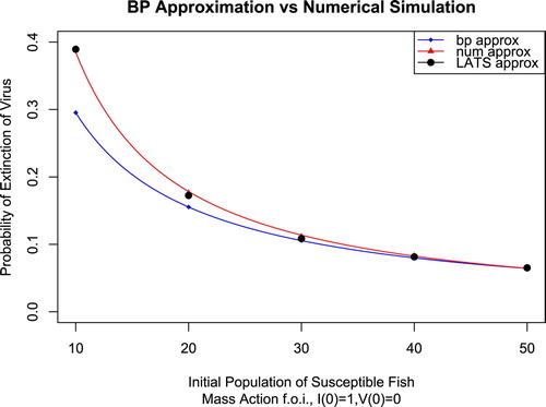
Using LATS to approximate the probability of extinction faithfully captures the behaviour of $X_t$ near the disease-free distribution, including any nonlinear behaviour. As a result, the LATS approximation in Figure 1 remains accurate as β is varied. The fact that LATS detects nonlinear behaviour is one of the benefits of this technique.

Since $X_t$ is a non-explosive process, for both branching process approximation and LATS, we first pass to the embedded DTMC, which we denote $X_n$. We say an outbreak has occurred in $X_n$ when $I_n+V_n\ge \overline{I}+\overline{V}$, where $\overline{I},\overline{V}$ are the numbers of infected individuals and infectious doses of free-virus at the outbreak quasistationary distribution (equivalent to the endemic equilibrium of the deterministic model (15(15) $\begin{array}{rcl}\stackrel{.}{S}& =& S(\beta -\mu S)-S(I+V),\\ \stackrel{.}{I}& =& S(I+V)-\alpha I,\\ \stackrel{.}{V}& =& -\omega V+\delta I.\end{array}$(15) )). We say extinction has occurred when $I_t+V_t=0$. In Assumption (A1), above, we consider the set of initial states T and seek to approximate the probability of hitting a single set V. In this case, we let T be the singleton $\{x_0=(\overline{S},1,0\left)\right\}$ and define the sets $O=\left\{\right(S,I,V)\in {\mathbb{N}}^3|I+V\ge \overline{I}+\overline{V}\}$ and $E=\left\{\right(S,I,V)\in {\mathbb{N}}^3|I+V=0\}$ to be the sets associated with outbreak and extinction, respectively. The sets E and O are disjoint. It is therefore possible to treat them both as V is treated in (A1). Suppose $f\left(E\right)=e$ and $f\left(O\right)=o$. The result is the collapsed state space ${\mathcal{S}}_N\left(x_0\right)$, which consists of the 3 absorbing states e (associated with extinction), o (associated with outbreak), and g (associated with escape from the neighbourhood) and all remaining states are transient. By Theorem 3.7, (17) $\sum _{k=1}^N{h}_{(x_0;X)}^{\left(k\right)}\left(j\right)={\left({\mathcal{Q}}_N^N\right(x_0\left)\right)}_{x_{0}f\left(j\right)},\mathrm{for}j=E\mathrm{or}O.$(17) Since $f\left(E\right)=e$ and $f\left(O\right)=o$, by (4(4) $h_{(i;X)}\left(j\right)=\sum _{m=0}^{\mathrm{\infty }}{h}_{(i;X)}^{\left(m\right)}\left(j\right)=\underset{N\to \mathrm{\infty }}{lim}\sum _{m=0}^N{h}_{(i;X)}^{\left(m\right)}\left(j\right).$(4) ), it follows that the entries $\left({\mathcal{Q}}_N^N\right(x_0){)}_{x_{0}e}$ and $\left({\mathcal{Q}}_N^N\right(x_0){)}_{x_{0}o}$ increase $h_{(x_0;X)}\left(E\right)$ and $h_{(x_0;X)}\left(O\right)$, respectively. By construction, there is no $x_0,g$-path of length N in the graph induced by $Y_n$. Therefore, $\left({\mathcal{Q}}_N^N\right(x_0){)}_{x_{0}g}=0$. Table 2 illustrates the convergence of $\left({\mathcal{Q}}_N^N\right(x_0){)}_{x_{0}e}$ and $\left({\mathcal{Q}}_N^N\right(x_0){)}_{x_{0}o}$ to $h_{(x_0;X)}\left(E\right)$ and $h_{(x_0;X)}\left(O\right)$, respectively.

Table 2. This table illustrates the convergence of entries in the row associated with $x_0$ of ${\mathcal{Q}}_N^N\left(x_0\right)$ to the hitting probabilities $h_{(x_0;X)}\left(E\right)$ and $h_{(x_0;X)}\left(O\right)$.

N	$({\mathcal{Q}}_N^N{)}_{x_{{}_0}e}$	$({\mathcal{Q}}_N^N{)}_{x_{{}_0}o}$	$({\mathcal{Q}}_N^N{)}_{x_{{}_0}g}$
1	0.0154	0	0
10	0.1219	0.0002	0
15	0.1625	0.0028	0
20	0.1945	0.0121	0
25	0.2205	0.0306	0
30	0.2422	0.0582	0
35	0.2609	0.0932	0
40	0.2770	0.1330	0
45	0.2911	0.1752	0
50	0.3035	0.2177	0
100	0.3678	0.5041	0
200	0.3881	0.6048	0
300	0.3892	0.6104	0
400	0.3893	0.6107	0

Notes: For each N, e, o and g are the states in ${\mathcal{S}}_N\left(T\right),$ the state space of the LATS collapsed chain $Y_n$, associated to extinction, outbreak, and escape from the N-neighbourhood, respectively. Parameter values are $\beta =10,\mu =1,\alpha =3.3,\delta =1.3$ and $\omega =4$.

Theorem 3.5 shows that the LATS collapsed chain $Y_n$ approximates the probabilities of extinction and outbreak another way, as well. That is, (18) $h_{(x_0;X)}\left(j\right)-h_{(x_0;Y)}\left(f\right(j\left)\right)\le h_{(x_0;Y)}\left(g\right),\mathrm{for}j=E\mathrm{or}O.$(18) Since the LATS collapsed chain $Y_n$ is a finite absorbing chain, by Theorem 2.1, ${\mathcal{Q}}_N\left(x_0\right)$ has canonical form given by (6(6) $P=\left[\begin{array}{cc}I& 0\\ \left[2pt/2pt\right]C& D\end{array}\right],$(6) ) and $h_{(x_0;Y)}\left(j\right)=(H{)}_{x_{0}j}$ for j=e,o or g and where $H=(I-D{)}^{-1}C$. In applications, approximating hitting probabilities with respect to $X_n$ using the LATS collapsed chain $Y_n$ via entries of the matrix H may converge faster and with less computational expense than approximating via the $N^{th}$ power of the matrix ${\mathcal{Q}}_N\left(x_0\right)$. This is illustrated in Table 3.

Table 3. This table illustrates the convergence of entries in the row associated with $x_0$ of $H=(I-D{)}^{-1}C$ to the hitting probabilities $h_{(x_0;X)}\left(E\right)$ and $h_{(x_0;X)}\left(O\right)$.

N	$(H{)}_{x_{{}_0}e}$	$(H{)}_{x_{{}_0}o}$	$(H{)}_{x_{{}_0}g}$
1	0.0283	0	0.9717
10	0.3470	0.3645	0.2885
15	0.3892	0.5905	0.0202
20	0.3893	0.6102	0.0005
25	0.3893	0.6107	0
30	0.3893	0.6107	0

Notes: For each N, e, o and g are the states in ${\mathcal{S}}_N\left(T\right),$ the state space of the LATS collapsed chain $Y_n$, associated with extinction, outbreak, and escape from the N-neighbourhood, respectively. The probability of escape does not actually reach 0, but does become so small as to be negligible for the purpose of numerical calculations. Parameter values are the same as those used in Table 2.

The results in Table 3 illustrate that for N=25, the probability that realizations with the initial state $x_0$ in the LATS collapsed chain $Y_n$ leave the N-neighbourhood before hitting the absorbing states associated with outbreak or escape is so small as to be negligible. Therefore, the LATS approximation $Y_n$ is an accurate representation of the embedded DTMC $X_n$ near the initial state $x_0$ for $N\ge 25$. Furthermore, in Table 3, the probability of extinction converges faster (for smaller N) than the probability of outbreak. This means that realizations with the initial state $x_0$ that lead to extinction are more likely to remain close to $x_0$ than those that lead to outbreak. This is reasonable, since the initial state $x_0$ is one transition in $X_n$ from the subspace $E\subset S$ associated with extinction, as evident from the first row of Table 2. Nevertheless, the fact that LATS approximation gives insight into the behaviour of $X_n$ at such fine resolution is another benefit of the technique.

5. Locally deployed disease control

In this section, we consider 2 small communities coupled together by migration. This metapopulation experiences a disease outbreak in which infected individuals become fully susceptible immediately upon recovery. First, a deterministic SIS model in the form of a system of nonlinear ODEs is proposed and analysed, then a related CTMC is developed. Consider the following hypothetical: suppose that both patches are at risk of outbreak in the sense that their patch type reproduction numbers are greater than 1, with patch 2 at higher risk than patch 1. Suppose that patch 1 has the resources to deploy disease control to reduce the rate of infection by $20\mathrm{\%}$, but can only be deployed in one patch. We consider the strategies of deployment in patch 1 only, or patch 2 only, and show which strategy minimizes the basic reproduction number for a particular choice of parameters. LATS is used to determine the optimal strategy for control in the CTMC, taking into account outcome preferences of decision makers.

First we consider the following deterministic two-patch SIS model: (19) $\begin{array}{rcl}\dot{\phantom{a}}{S}_1& =& -{\beta }_1\frac{S_1{I}_1}{N_1}+{\gamma }_1{I}_1+d(S_2-S_1),\\ {\dot{I}}_1& =& {\beta }_1\frac{S_1{I}_1}{N_1}-{\gamma }_1{I}_1+d(I_2-I_1),\\ {\dot{S}}_2& =& -{\beta }_2\frac{S_2{I}_2}{N_2}+{\gamma }_2{I}_2+d(S_1-S_2),\\ {\dot{I}}_1& =& {\beta }_2\frac{S_2{I}_2}{N_2}-{\gamma }_2{I}_2+d(I_1-I_2),\end{array}$(19) where, in patch i, $S_i$ is the number of susceptible individuals, $I_i$ is the number of infected individuals, $N_i=S_i+I_i$ is the total number of individuals, ${\beta }_i$ is the rate of infection and ${\gamma }_i$ is the rate of recovery for i=1,2. The rate of migration between patches is d and $N=N_1+N_2$ is the total number of individuals in the system. This model corresponds to the model studied in [37] with n=2, ${\alpha }_1={\alpha }_2=0$ and $d_{12}=d_{21}=d$. When $I_1=I_2=0$, the system admits the disease-free steady state $S_1=S_2=N/2$. Following [37], the basic reproduction number is (20) ${\mathcal{R}}_0=\frac{{\beta }_1({\gamma }_2+d)+{\beta }_2({\gamma }_1+d)+\sqrt{\left({\beta }_1\right({\gamma }_2+d)-{\beta }_2({\gamma }_2+d){)}^2+4d^2{\beta }_1{\beta }_2}}{2\left[\right({\gamma }_1+d\left)\right({\gamma }_2+d)-d^2]}.$(20) The patch type reproduction number is given by ${\mathcal{R}}_{0i}={\beta }_i/{\gamma }_i$ for i=1,2 and corresponds to the basic reproduction number in each patch in the absence of migration. Suppose that ${\beta }_1=0.4,{\beta }_2=0.5,{\gamma }_1=0.2,{\gamma }_2=0.1,$ and d=0.1. Then ${\mathcal{R}}_{01}=2$, ${\mathcal{R}}_{02}=5$ and ${\mathcal{R}}_0\approx 3.4358$. Now we modify system (19(19) $\begin{array}{rcl}\dot{\phantom{a}}{S}_1& =& -{\beta }_1\frac{S_1{I}_1}{N_1}+{\gamma }_1{I}_1+d(S_2-S_1),\\ {\dot{I}}_1& =& {\beta }_1\frac{S_1{I}_1}{N_1}-{\gamma }_1{I}_1+d(I_2-I_1),\\ {\dot{S}}_2& =& -{\beta }_2\frac{S_2{I}_2}{N_2}+{\gamma }_2{I}_2+d(S_1-S_2),\\ {\dot{I}}_1& =& {\beta }_2\frac{S_2{I}_2}{N_2}-{\gamma }_2{I}_2+d(I_1-I_2),\end{array}$(19) ) to include parameters ${\theta }_1$ and ${\theta }_2$ related to the control. The new system is given by (21) $\begin{array}{rcl}{\dot{S}}_1& =& -{\theta }_1{\beta }_1\frac{S_1{I}_1}{N_1}+{\gamma }_1{I}_1+d(S_2-S_1),\\ {\dot{I}}_1& =& {\theta }_1{\beta }_1\frac{S_1{I}_1}{N_1}-{\gamma }_1{I}_1+d(I_2-I_1),\\ {\dot{S}}_2& =& -{\theta }_2{\beta }_2\frac{S_2{I}_2}{N_2}+{\gamma }_2{I}_2+d(S_1-S_2),\\ {\dot{I}}_1& =& {\theta }_2{\beta }_2\frac{S_2{I}_2}{N_2}-{\gamma }_2{I}_2+d(I_1-I_2),\end{array}$(21) which corresponds to system (19(19) $\begin{array}{rcl}\dot{\phantom{a}}{S}_1& =& -{\beta }_1\frac{S_1{I}_1}{N_1}+{\gamma }_1{I}_1+d(S_2-S_1),\\ {\dot{I}}_1& =& {\beta }_1\frac{S_1{I}_1}{N_1}-{\gamma }_1{I}_1+d(I_2-I_1),\\ {\dot{S}}_2& =& -{\beta }_2\frac{S_2{I}_2}{N_2}+{\gamma }_2{I}_2+d(S_1-S_2),\\ {\dot{I}}_1& =& {\beta }_2\frac{S_2{I}_2}{N_2}-{\gamma }_2{I}_2+d(I_1-I_2),\end{array}$(19) ) when ${\theta }_1={\theta }_2=1$. The strategy of deploying disease control in patch 1 corresponds to $({\theta }_1,{\theta }_2)=(0.8,1)$ and the complementary strategy corresponds to $({\theta }_1,{\theta }_2)=(1,0.8)$. The effect these strategies have on ${\mathcal{R}}_0$ and ${\mathcal{R}}_{0i}$ for i=1,2 is found in Table 4. Clearly, the strategy of deploying control in patch 2 minimizes ${\mathcal{R}}_0$ as well as minimizing the sum of the patch-specific reproduction numbers, ${\mathcal{R}}_{01}+{\mathcal{R}}_{02}$. Regardless of which strategy is chosen, ${\mathcal{R}}_0>1$ and the disease persists [27].

Table 4. Patch-specific and overall reproduction numbers for no control, control deployed in patch 1 only and control deployed in patch 2 only.

$({\theta }_1,{\theta }_2)$	${\mathcal{R}}_{01}$	${\mathcal{R}}_{02}$	${\mathcal{R}}_0$
(1,1)	2	5	3.4358
(0.8,1)	1.6	5	3.3146
(1,0.8)	2	4	2.8944

If d=0, then the system decouples and the basic reproduction number in a single patch is given by the patch type reproduction number ${\mathcal{R}}_{0i}={\beta }_i/{\gamma }_i$, for i=1,2. For $N_i$ sufficiently large, the probability of extinction following the introduction of a single infected individual is given by the GWbp approximation $q=1/{\mathcal{R}}_{0i}={\gamma }_i/{\beta }_i$, a decreasing function of ${\mathcal{R}}_{0i}$ [3,51].

In order to investigate what happens at small population size we consider the CTMC $X_t=\left(S_1\right(t),I_1(t),S_2(t),I_2(t\left)\right)$ with the infinitesimal transition probabilities $p_{ij}\left(\mathrm{\Delta }t\right)=P(X_{t+\mathrm{\Delta }t}=j|X_t=i)=\sigma (i,j)\mathrm{\Delta }t+o\left(\mathrm{\Delta }t\right)$ and associated rates $\sigma (i,j)$ found in Table 5.

Table 5. State transitions and rates for the two-patch SIS CTMC, $X_t$

Description	Transition	Rate $\sigma (i,j)$
Infection ·$S_1$	$S_1,I_1\mapsto S_1-1,I_1+1$	${\theta }_1{\beta }_1\frac{S_1{I}_1}{N_1}$
Recovery ·$I_1$	$S_1,I_1\mapsto S_1+1,I_1-1$	${\gamma }_1{I}_1$
Infection ·$S_2$	$S_2,I_2\mapsto S_2-1,I_2+1$	${\theta }_2{\beta }_2\frac{S_2{I}_2}{N_2}$
Recovery ·$I_2$	$S_2,I_2\mapsto S_2+1,I_2-1$	${\gamma }_2{I}_2$
Migration ·$S_1$	$S_1,S_2\mapsto S_1-1,S_2+1$	$d{S}_1$
Migration ·$I_1$	$I_1,I_2\mapsto I_1-1,I_2+1$	$d{I}_1$
Migration ·$S_2$	$S_1,S_2\mapsto S_1+1,S_2-1$	$d{S}_2$
Migration ·$I_2$	$I_1,I_2\mapsto I_1+1,I_2-1$	$d{I}_2$

Consider the two-patch SIS CTMC, $X_t,$ with the parameters ${\beta }_1=0.4,{\beta }_2=0.5,{\gamma }_1=0.2,{\gamma }_2=0.1,d=0$ and control strategy $({\theta }_1,{\theta }_2)$. Since d=0 the two patches are decoupled and ${\dot{N}}_i=0$ for i=1,2. Suppose there are initially 10 individuals in patch 1 and 5 individuals in patch 2. Using LATS, we determine the probability of extinction ${\mathbb{P}}_{0i}$ in patch i from the initial state $(9,1)$ in patch 1 and $(4,1)$ in patch 2 with and without control. As noted above, Whittle showed that in this case the GWbp approximation of the probability of extinction in patch i is the reciprocal of the patch reproduction number [51]. The results of LATS approximation of the probability of extinction are reported alongside the patch reproduction numbers and the reciprocals of the patch reproduction numbers in Table 6. The results of the experiments reported in Table 6 coincide with the hypothesis that the probability of extinction in a single patch is monotone in ${\mathcal{R}}_0$ for small populations as well.

Table 6. Patch i reproduction numbers (${\mathcal{R}}_{0i}$) and GWbp probabilities of extinction (${}^1{/}_{{\mathcal{R}}_{0i}}$) and LATS probabilities of extinction (${\mathbb{P}}_{0i}$) from the initial state $(9,1)$ in patch i=1 and $(4,1)$ in patch i=2 with and without control.

$({\theta }_1,{\theta }_2)$	${\mathcal{R}}_{01}$	${\mathcal{R}}_{02}$	$\frac{1}{{\mathcal{R}}_{01}}$	$\frac{1}{{\mathcal{R}}_{02}}$	${\mathbb{P}}_{01}$	${\mathbb{P}}_{02}$
$(1,1)$	2	5	0.5	0.2	0.5758	0.2727
$(0.8,0.8)$	1.6	4	0.625	0.24	0.6325	0.3439

Note: Parameter values are given by ${\beta }_1=0.4,{\beta }_2=0.5,{\gamma }_1=0.2,{\gamma }_2=0.1,d=0$.

Now let d=0.1 so that the two patches form a metapopulation. Let us return to the hypothetical that residents of patch 1 have resources available to deploy a control strategy that reduces the rates of infection in a single patch. The residents of patch 1 wish to deploy the control in the patch that yields the greatest benefit to themselves. To account for this preference, we want to calculate the probability of extinction in patch 1 only from the initial state $x_0=(10,1,1,3)$. This is the state of the system if patch 1 is at its single patch quasistationary disease-free state $(10,0)$, patch 2 is at its single patch quasistationary endemic state $(1,4)$ and a single infected individual migrates from endemic patch 2 to patch 1 as the rate of movement between patches, d, becomes positive. Recall that the state space S of $X_t$ is the subset $S=\left\{\right(S_1,I_1,S_2,I_2\left)\right\}\subset {\mathbb{N}}^4$ with the property that $S_1+I_1+S_2+I_2=S_1\left(0\right)+I_1\left(0\right)+S_2\left(0\right)+I_2\left(0\right)$, i.e. that the total population is preserved. Let $A=\left\{\right(S_1,I_1,S_2,I_2)\in S:I_1=0\}$ be the subset of S associated with the extinction of the disease in patch 1 only and let $E=\left\{\right(S_1,I_1,S_2,I_2)\in S:I_1=I_2=0\}$ be the subset of S associated with total extinction of the disease. Then $E\subset A$. Define the probability of partial extinction in patch 1 to be the probability of hitting the set A. Since d>0, the event $X_t=a$ for $a\in A\setminus E$ is transient. However, we take it as an indicator of the disease risk in patch 1. Let $X_n$ be the embedded DTMC. We use LATS as described in (A1) with V =A to approximate $h_{(x_0;X)}\left(A\right)$ and again with V =E to approximate $h_{(x_0;X)}\left(E\right)$. Results in Table 7 show that strategy $({\theta }_1,{\theta }_2)=(0.8,1)$, corresponding to deployment in patch 1, optimizes patch 1 partial extinction, $h_{(A;X)}\left(x_0\right)$. In contrast, the probability of total extinction, $h_{(E;X)}\left(x_0\right)$, indicates deployment in patch 2 optimizes total extinction of the disease.

Table 7. Probability of partial extinction in patch 1 only and total extinction from initial state $x_0=(10,1,1,3).$

$({\theta }_1,{\theta }_2)$	$h_{(A;X)}\left(x_0\right)$	$h_{(E;X)}\left(x_0\right)$
(1,1)	0.6157	0.0623
(0.8,1)	0.7095	0.0940
(1,0.8)	0.6591	0.1077

Obviously, these are conflicting results. In order to make sense of them, we consider the classical setting in which a single infected individual appears in one patch or the other and calculate the probability of total extinction. The disease-free quasistationary distribution of the two-patch model is $(7.5,0,7.5,0)$, which is not a state of the system. Therefore, we expect $X_t$ to fluctuate between the states $(8,0,7,0)$ and $(7,0,8,0)$ when it is near the quasistationary distribution. We therefore consider the probability of extinction from the initial states $x_1=(7,1,7,0)$ and $x_2=(7,0,7,1)$. These probabilities are reported in Table 8.

Table 8. The probability of extinction from initial state $x_1=(7,1,7,0)$ and $x_2=(7,0,7,1)$.

$({\theta }_1,{\theta }_2)$	$h_{(x_1;X)}\left(E\right)$	$h_{(x_2;X)}\left(E\right)$
(1,1)	0.5183	0.3298
(0.8,1)	0.5868	0.3602
(1,0.8)	0.5567	0.4151

The results in Table 8 provide insight into the effect of the different control strategies. First, disease control measures deployed in a single patch promotes disease extinction in both patches. The probability of partial extinction in patch 1 given by $h_{(A;X)}\left(x_0\right)$ reported in Table 7 and $h_{(E;X)}\left(\right(7,1,7,0\left)\right)$ reported in Table 8 reflects a bias towards patch 1, while $h_{(E;X)}\left(\right(7,0,7,1\left)\right)$ reflects a bias towards patch 2. From the perspective of a given patch, the optimal outcome is a result of deploying control measures in that patch, which may or may not coincide with minimizing ${\mathcal{R}}_0$. The product of column $h_{(x_1;X)}\left(E\right)$ and column $h_{(x_2;X)}\left(E\right)$ can be viewed as giving a global perspective. From this perspective, it is still optimal to deploy control measures in a way that also minimizes ${\mathcal{R}}_0$. Partial extinction probabilities, like $h_{(x_0;X)}\left(A\right)$, may be useful tools for decision-making in the context of heterogeneous control in metapopulations. In addition to being a potentially useful indicator for heterogeneous control problems, $h_{(x_0;X)}\left(A\right)$ cannot be calculated using branching process approximation. The very fact that we have been able to calculate this probability using LATS illustrates another benefit of the technique, namely, that it is suited to approximating hitting problems in general.

6. Discussion

The LATS technique combines localization and collapsing of Markov chains to reduce a DTMC on a countably infinite state space to a finite absorbing Markov chain. It is a robust tool for approximating general hitting probabilities for typical chains when the local neighbourhood is sufficiently large. However, increasing the size of a neighbourhood comes at the cost of increasing computational expense, particularly if the degree of the induced graph is large. LATS is shown to be effective in some cases where branching process techniques are not suitable. This is due, in part, to the fact that LATS captures nonlinear behaviour of the Markov chain it seeks to approximate. In addition to solving the general hitting problem, LATS also gives information about the number of transitions in a path as well as the likelihood of long sojourns. Therefore, it is a valuable addition to the set of tools used to analyse stochastic models of real world phenomena.

In Section 5, partial extinction probabilities are shown to have the potential to help inform deployment of spatially heterogeneous disease control strategies. There are likely other interesting biological questions that can be formulated as general hitting problems. LATS is well suited to provide approximations for these problems.

In the context of heterogeneous control strategies, outcome preferences are important drivers of decision-making. Standard techniques to calculate probability of extinction may not be the ideal way to account for this. Formulating hitting problems that account for preference, such as partial extinction probabilities, may be useful to optimize decision-making subject to constrains.

Disclosure statement

No potential conflict of interest was reported by the author.

ORCID

Evan Milliken  http://orcid.org/0000-0003-1268-9020

Additional information

Funding

This work was supported in part by NSF grant DMS-1515661 (Division of Mathematical Sciences) awarded to Maia Martcheva as PI and Robert D. Holt as Co-PI.

References

- L.J.S. Allen, An Introduction to Stochastic Processes with Applications to Biology, Pearson, Upper Saddle River, NJ, 2003.
- L.J.S. Allen and A.M. Burgin, Comparison of deterministic and stochastic SIS and SIR models in discrete time, Math. Biosci. 163(1) (2000), pp. 1–33.
- L.J.S. Allen and G.E. Lahodny, Extinction thresholds in deterministic and stochastic epidemic models, J. Biol. Dyn. 6(2) (2012), pp. 590–611.
- L.J.S. Allen and E.J. Schwartz, Free-virus and cell-to-cell transmission in models of equine infectious anemia virus infection, Math. Biosci. 270 (2015), pp. 237–248.
- L.J.S. Allen and P. van den Driessche, Relations between deterministic and stochastic thresholds for disease extinction in continuous- and discrete-time infectious disease models, Math. Biosci. 243(1) (2013), pp. 99–108.
- J. Arino, Diseases in metapopulations, in Modeling and Dynamics of Infectious Diseases, Vol. 11, Z. Ma, Y. Zhou, and J. Wu, eds., World Scientific, New Jersey, 2009, pp. 65–123.
- J. Arino, Spatio-temporal spread of infectious pathogens of humans, Infect. Dis. Model. 2(2) (2017), pp. 218–228.
- J. Arino and S. Portet, Epidemiological implications of mobility between a large urban centre and smaller satellite cities, J. Math. Biol. 71(5) (2015), pp. 1243–1265.
- J. Arino and P. van den Driessche, A multi-city epidemic model, Math. Popul. Stud. 10(3) (2003), pp. 175–193.
- F. Arrigoni and A. Pugliese, Limits of a multi-patch SIS epidemic model, J. Math. Biol. 45(5) (2002), pp. 419–440.
- N.T.J. Bailey, The Mathematical Theory of Infectious Diseases and Its Applications, 2nd ed., Hafner, New York, 1975.
- F.G. Ball and P. Donnelly, Strong approximations for epidemic models, Stoch. Proc. Appl. 55(1) (1995), pp. 1–21.
- F. Ball, B. Tom, and L. Owen, Stochastic multitype epidemics in a community of households: Estimation and form of optimal vaccination schemes, Math. Biosci. 191(1) (2004), pp. 19–40.
- M. Behzad and G. Chartrand, Introduction to the Theory of Graphs, Allyn and Bacon, Inc., Boston, 1971.
- M. Bóna, A walk through combinatorics: An introduction to enumeration and graph theory, World Scientific, New Jersey, 2013.
- C.J. Burke and M. Rosenblatt, A Markovian function of a Markov chain, Ann. Math. Statist. 29(4) (1958), pp. 1112–1122.
- A. Dey and A. Mukherjea, Collapsing of non-homogeneous Markov chains, Statist. Probab. Lett. 84(1) (2014), pp. 140–148.
- T. Dhirasakdanon, H.R. Thieme, and P. Van Den Driessche, A sharp threshold for disease persistence in host metapopulations, J. Biol. Dyn. 1(4) (2007), pp. 363–378.
- O. Diekmann, J. Heesterbeek, and J. Metz, On the definition and computation of the basic reproduction ratio R0 in models of infectious disease in heterogeneous populations, J. Math. Biol. 28 (1990), pp. 365–382.
- R. Durrett, Essentials of Stochastic Processes, 2nd ed., Springer-Verlag, New York, 2012.
- K. Falk, E. Namork, E. Rimstad, S. Mjaaland, and B.H. Dannevig, Characterization of infectious salmon anemia virus, an orthomyxo-like virus isolated from Atlantic salmon (Salmo salar L.), J. Virol. 71(12) (1997), pp. 9016–23.
- I.I. Gikhman and A.V. Skorokhod, Introduction to the Theory of Random Processes, Dover, Mineola, NY, 1996.
- S.A. Gourley, H.R. Thieme, and P. van den Driessche, Stability and persistence in a model for bluetongue dynamics, SIAM J. Appl. Math. 71(4) (2011), pp. 1280–1306.
- A. Gray, D. Greenhalgh, L. Hu, X. Mao, and J. Pan, A stochastic differential equation SIS epidemic model, SIAM J. Appl. Math. 71(3) (2011), pp. 876–902.
- J. Hachigian, Collapsed Markov chains and the Chapman-Kolmogorov equation, Ann. Math. Statist. 34(1) (1963), pp. 233–237.
- T.E. Harris, The Theory of Branching Processes, Springer-Verlag, Berlin, 1963.
- A. Iggidr, G. Sallet, and B. Tsanou, Global stability analysis of a metapopulation SIS epidemic model, Math. Popul. Stud. 19(3) (2012), pp. 115–129.
- M. Jesse, R. Mazzucco, U. Dieckmann, H. Heesterbeek, and J.A.J. Metz, Invasion and persistence of infectious agents in fragmented host populations, PLoS ONE 6(9) (2011).
- S. Karlin and H.M. Taylor, A First Course in Stochastic Processes, 2nd ed., Academic Press, New York, 1975.
- M.J. Keeling, Metapopulation moments: Coupling, stochasticity and persistence, J. Anim. Ecol. 69(5) (2000), pp. 725–736.
- M.J. Keeling, C.A. Gilligan, and M.J. Keeling, Metapopulation dynamics of bubonic plague, Nature 407(6806) (2000), pp. 903–906.
- M.J. Keeling and J.V. Ross, On methods for studying stochastic disease dynamics, J. R. Soc. Interface 5(19) (2008), pp. 171–181.
- J.G. Kemeny and J.L. Snell, Finite Markov Chains, Springer-Verlag, New York, 1976.
- W.O. Kermack and A.G. McKendrick, Contributions to the mathematical theory of epidemics – I, Proc. R. Soc. A 115(772) (1927), pp. 700–721.
- A. Khanafer and B. Tamer, An optimal control problem over infected networks, Proceedings of the International Conference of Control, Dynamic Systems, and Robotics, Ottawa, Ontario, Canada, 2014.
- A.L. Krause, L. Kurowski, K. Yawar, and R.A. Van Gorder, Stochastic epidemic metapopulation models on networks: SIS dynamics and control strategies, J. Theor. Biol. 449 (2018), pp. 35–52.
- G.E. Lahodny and L.J.S. Allen, Probability of a disease outbreak in stochastic multipatch epidemic models, Bull. Math. Biol. 75(7) (2013), pp. 1157–1180.
- E. Milliken, The probability of extinction of infectious salmon anemia virus in one and two patches, Bull. Math. Biol. 79 (2017), pp. 2887–2904.
- E. Milliken and S.S. Pilyugin, A model of infectious salmon anemia virus with viral diffusion between wild and farmed patches, DCDS-B 21(6) (2016), pp. 1869–1893.
- J.R. Norris, Markov Chains, Cambridge University Press, New York, 1997.
- M.A. Pinsky and S. Karlin, Introduction to Stochastic Modeling, Academic Press, Boston, 2011.
- M. Roseblatt, Functions of a Markov process that are Markovian, J. Math. Mech. 8(4) (1959), pp. 585–596.
- M. Rosenblatt, Random Processes, Oxford University Press, New York, 1962.
- R. Ross, An application of the theory of probabilities to the study of a priori pathometry. Part I, Proc. R. Soc. A 92(638) (1916), pp. 204–230.
- P. van den Driessche and J. Watmough, Reproduction numbers and sub-threshold endemic equilibria for compartmental models of disease transmission, Math. Biosci. 180 (2002), pp. 29–48.
- S. Vike, S. Nylund, and A. Nylund, ISA virus in Chile: Evidence of vertical transmission, Arch. Virol. 154(1) (2009), pp. 1–8.
- W. Wang and X.-Q. Zhao, An epidemic model in a patchy environment, Math. Biosci. 190(1) (2004), pp. 97–112.
- H.W. Watson and F. Galton, On the probability of extinction of families, J. Anthropol. Inst. GB Ireland 4 (1875), pp. 138–144.
- D.B. West, Introduction to Graph Theory, Prentice Hall, Upper Saddle River, NJ, 1996.
- R.W. West and J.R. Thompson, Models for the simple epidemic, Math. Biosci. 141 (1997), pp. 29–39.
- P. Whittle, The outcome of a stochastic epidemic – a note on Bailey's paper, Biometrika 42 (1955), pp. 116–122.