
 ?Mathematical formulae have been encoded as MathML and are displayed in this HTML version using MathJax in order to improve their display. Uncheck the box to turn MathJax off. This feature requires Javascript. Click on a formula to zoom.
ABSTRACT
A simplified stochastic control model for optimization of logistic dynamics with the control-dependent carrying capacity, which is motivated by a recent algae population management problem in the river environment, is presented. Solving the optimization problem reduces to finding a solution to a non-local first-order differential equation called tt–Jacobi–Bellman (HJB) equation. It is shown that the HJB equation has a unique viscosity solution and that the solution can be approximated with a finite difference scheme. Asymptotic estimates of the solution and the optimal control are derived and compared with numerical solutions. Finally, parameter dependence of the optimal control is examined numerically with implications to river environmental management.
1. Introduction
This paper focuses on a new stochastic control model and its application to algae management in rivers, in which modelling and control of population dynamics play central roles. Not limited to this problem, mathematical modelling of population dynamics in natural environment is a heart of ecological management [Citation52]. Recent examples include invasive species management [Citation28], tracking predator-prey dynamics for biological conservation [Citation50], and sustainable fisheries management [Citation19]. The population dynamics is often inherently stochastic mainly due to unresolved nonlinearities involved in the ecological and environmental processes [Citation31]. Stochastic process models like the stochastic differential equations (SDEs) [Citation42] are adequate mathematical tools for modelling and control of such dynamics.
SDEs serve as simple mathematical models for a variety of population dynamics and related environmental and ecological problems. Mandal et al. [Citation38] considered phytoplankton dynamics with a system of nonlinear SDEs for analysis of noise-dependent population extinction. Mau et al. [Citation39] presented a multiplicative jump process model for minimum mathematical description of salt and contaminants dynamics in soil environment. Sanz and Alonso [Citation48] discussed an approximate aggregation technique for simplifying an SDE-based heterogeneous population dynamics model. Allen [Citation3] derived a stochastic partial differential equation that governs size- and age-dependent population dynamics in noisy environment from a discretized SDE counterpart.
Management of population dynamics can be addressed in the framework of stochastic control [Citation21,Citation43]. In this framework, the system to be controlled is often described with a system of SDEs. With a performance index to be minimized or maximized, owing to the dynamic programming principle, finding the optimal control reduces to solving a Hamilton–Jacobi–Bellman (HJB) equation: a degenerate elliptic or parabolic equation whose functional form is problem-dependent [Citation21]. Both mathematical and numerical approaches have been addressed for analysis of HJB equations in many problems, ranging from financial [Citation17], economic [Citation1], and insurance problems [Citation14] to biological [Citation62], environmental [Citation12], and ecological problems [Citation60]. Neilan et al. [Citation40] reviewed recent progresses of numerical schemes for solving HJB and related nonlinear differential equations.
The logistic equation having the form
(1)
(1) is one of the most widely-used mathematical models for population growth [Citation11]. Here,
is the time,
is the intrinsic growth rate,
is the carrying capacity, and
is the population at the time
. Starting from the basic equation (1), many variants like the equation with the uncertain parameters [Citation18], that with stochastic intrinsic growth rate [Citation36], and that having noise-driven carrying capacity [Citation4], have been proposed and analysed. Our problem also starts from the basic Equation (1) as explained below.
In this paper, we present a prompt report on modelling and control of a stochastic logistic equation-based model with an emphasis on algae population management in river environment [Citation35,Citation56]. Dense and wide spreading of the invasive macrophytes and benthic algae, such as Egeria densa [Citation26,Citation51] and Cladophora glomerata [Citation64,Citation66], has been an urgent issue. The motivation of the present mathematical model is the reports on the non-trivial dependence of the in-river population of E. densa on the flow speed [Citation27,Citation30]. They reported that the stable equilibrium of the algae population is a concave unimodal function of the flow speed, which cannot be reproduced with the conventional mathematical models [Citation22,Citation55,Citation63,Citation64] based on the logistic-type model
(2)
(2) where
is the flow speed and
is the decay coefficient of the algae population as an increasing function of
. The model (2) having the constant parameters
and
is able to reproduce the population decay due to high-speed river flows [Citation35,Citation55], but the reported unimodal nature cannot be reproduced with the model (2) unless the flow-dependent
and/or
are employed. In river environment, the flow discharge, or flow speed, are the variables controlled by human through operating hydraulic structures like dams and weirs [Citation32]. Therefore, from the viewpoint of algae population management [Citation63,Citation64], controlling the population dynamics in a river environment can be seen as a stochastic optimization problem of a logistic-type equation having control-dependent parameters. So far, such a mathematical approach has not been examined.
The objectives of this paper are thus formulation and analysis of a stochastic optimization problem based on the logistic-type population dynamics with a control-dependent carrying capacity. As a first step of the new mathematical modelling, the focus of this paper is on analysis of a simplified problem rather than model application to practical cases. Solving the optimization problem reduces to finding a solution to an associated HJB equation, which is a non-local first-order differential equation. It is shown that the HJB equation has a unique viscosity solution: an appropriate weak solution for this kind of equations [Citation16]. The HJB equation is not exactly-solvable as in those arising in other ecological problems [Citation59,Citation60], but asymptotic estimates of its solution are found. A finite difference scheme for approximation of the solution is then presented. The model is finally applied to management of benthic algae to see dependence of the optimal control on the parameters in the population dynamics and performance index.
The rest of this paper is organized as follows. Section 2 presents the mathematical model focused on in this paper and derives the HJB equation. Its mathematical analysis is carried out in this section as well. Section 3 presents the finite difference scheme for discretization of the HJB equation and its mathematical analysis results. Section 4 is devoted to numerical computation of the HJB equation focusing on the algae population management problem. Section 5 concludes this paper and presents future perspectives of our research. The appendix contains the proofs of propositions stated in Sections 2 and 3.
2. Mathematical model
The population dynamics model and performance index are presented and the HJB equation to be solved is derived and analysed. The model is firstly formulated in a generalized manner, and a specific problem related to the benthic algae management is formulated in Section 2.5.
2.1. Problem setting
A logistic-type model for describing control-dependent population dynamics in stochastic environment is presented. The time is denoted as . The population at each time
is a non-negative variable denoted as
. The population dynamics is described by an SDE driven by a multiplicative jump noise modelled with the standard Poisson process
(
) with the intensity parameter
and the jump size
, where
represents the mean waiting time between each successive jumps. For the benthic algae population management, the noise corresponds to flood events such that a large part of the population is suddenly removed from riverbed. The parameter
corresponds to the magnitude of the flood events. The process
is defined on the usual complete probability space. A natural filtration generated by
is denoted as
[Citation43]. The control variable to be optimized is a measurable variable of the time
, which is denoted as
at each
. As in standard problem settings [Citation43],
is assumed to be valued in the compact set
with
, and to be adapted to
. Consequently, we define the set of admissible controls as
, which is a collection of all measurable continuous-time processes
(
) adapted to the filtration
.
2.2. Population dynamics to be controlled
The SDE governing the evolution of is set as
(3)
(3) subject to the initial condition
. Here,
is the carrying capacity of the population,
is the intrinsic growth rate, and
is the decay coefficient. The coefficients
,
, and
are assumed to be Lipschitz continuous functions in
. Assume
without significant loss of generality.
The SDE (3) contains the four terms. The left-hand side is the increment of the population in the infinitesimal time interval, the first term in the right-hand side is the logistic growth term, the second term represents the gradual population decay, and the third term represents the sudden population decay. In the context of the benthic algae population management, the second term is due to regular river flows, while the third term is due to flood events. At each jump of
,
suddenly decreases as
(4)
(4) By the initial condition and the sign and form of each term of (3), it is shown that the process
satisfies
for
. The range of the process
is therefore compact under the assumption and is denoted as
.
Remark 2.1:
Solutions to the SDE (3) can have a unique solution for some controls that are admissible since at least the constant controls such that
with a constant
are admissible. This is because of the standard discussion for the uniqueness result without the jump term following Theorem 1 of Lv et al. [Citation37] for such a control, since the noise term does not affect uniqueness of the solutions. In addition,
for
a.s. if
, because of the relationship (4) at each jump and the fact that the jump process is a standard Poisson process. Therefore, we have
a.s. for
, where
. Strong uniqueness of solutions to the SDE (3) should be studied from a mathematically more rigorous viewpoint, but we do not address this issue since our mathematical focus is on the controlling part (HJB equation).
Remark 2.2:
The SDE (3) can be extended to models with continuous noises [Citation49], wider class of jump terms [Citation33], and model ambiguity [Citation24]. These models would be practically and theoretically of more interest but may be less analytically tractable.
Remark 2.3:
The SDE (3) can also be considered in the context of optimal control of piecewise deterministic Markov processes [Chapter 8 of Citation9] since it is driven by a standard Poisson process.
2.3. Performance index to be minimized
The performance index is a functional of the initial condition
and an admissible control
(
), which is set in this paper as
(5)
(5) where
is the expectation,
is the discount rate, and
is a non-negative and Lipschitz continuous function with respect to the first argument in
and the second argument in
. Therefore,
is Lipschitz continuous in the compact set
. The function
models the cost of the management and the disutility caused by the existence of the population [Citation58,Citation63–65] in a general manner. On the function
, we assume that it is increasing with respect to the second argument, meaning that the disutility caused by the population is larger for larger population. In addition, it is assumed that
, meaning that no management problem arises if there is no population. The discount rate
measures perspective of the decision-maker, the manager of the population. The decision-maker has a shorter-term perspective when
is larger as in the conventional stochastic control problems [Citation10].
The minimized performance index with respect to controls
is the value function
in the sense of Markov control. This quantity is defined as
(6)
(6) In this paper, we restrict ourselves to consider Markovian control processes of the form
,
with some measurable function
in the set of admissible controls. The minimizer that archives
is called the optimal control
:
(7)
(7) The optimal control
is a function of the process
and hence a feed-back control. The goal of the present problem is to find
, which is addressed in this paper through solving an HJB equation presented in the next sub-section. Clearly,
is non-negative and bounded because of the inequality
(8)
(8)
2.4. HJB equation
Introduce the interval for the sake of brevity of descriptions. Application of the dynamic programming principle (Chapter 3 of Øksendal and Sulem [Citation43]) to (6) formally leads to the governing equation of
: the HJB equation
(9)
(9) subject to the boundary condition
, which is due to
(10)
(10) and the non-negativity (8). From the HJB equation (9), with an abuse of notation, the optimal control
for each
is obtained as
(11)
(11) which can be formally determined through the derivative
that exists almost everywhere inside
(See, proof of Proposition 2.1). In this sense, finding
, the quantity to be evaluated through tackling the optimal control problem, can be achieved through solving the HJB equation (9).
Unfortunately, HJB equations may not have classical solutions belonging to the function space in general because of their nonlinearities [Citation21]. Therefore, a weak notion of solutions, namely the concept of viscosity solutions [Citation16] is introduced. This definition harmonizes with uniqueness of solutions to the equation and its numerical discretization. Let
and
be spaces of upper- and lower- semicontiguous functions in
, respectively. Set
. Viscosity solutions to the HJB equation (9) are defined as follows [Citation5,Citation16,Citation21].
Definition 2.1:
A function
such that
A function
A bounded and continuous function
Now, we prove the following propositions, which are main mathematical results of this paper. They suggest that finding the optimal control through solving the HJB equation (9) is a mathematically rigorous approach for the present optimization problem.
Proposition 2.1:
The value function is a viscosity solution to the HJB equation (9).
Proposition 2.2:
The HJB equation (9) admits at most one viscosity solution.
Proposition 2.3:
The value function is the unique viscosity solution to the HJB equation (9).
Proposition 2.1 shows existence of solutions to the HJB equation (9), and their uniqueness is proved in Proposition 2.2. Proposition 2.3 is a consequence of Propositions 2.1 and 2.2. Uniqueness of viscosity solutions to HJB equations is not a trivial issue even for seemingly simple problems [Citation6,Citation67,Citation69].
2.5. Specific model for the algae population control
In this sub-section, the functional forms of the coefficients ,
,
, and
are specified for more detailed analysis. A motivation of considering control-dependent coefficients
and
is the recently-reported semi-quadratic formula between the stable population density
of E. densa and the flow speed
in a Japanese river [Citation27]
(14)
(14) with positive constants
,
, and
, which are identified from observations at several sampling stations in the river. In the context of the equations (2) or (3) (the control
is here identified as the flow speed
), assuming that the jumps are not so frequent such that a stable equilibrium of the population is well-established, we obtain
(15)
(15) Since it is physically reasonable to consider that the decay coefficient
is increasing with respect to the flow speed
, consistency between (14) and (15) cannot be obtained unless we assume flow dependence of
and
. At least, it cannot be obtained if both
and
are constants.
In this paper, for the sake of simplicity of analysis, we consider the case is a constant while
. This relationship can be justified if
is positive and increasing with respect to
, at least for not large
such that E. densa are critically removed from the riverbed [Citation64]. The increasing nature of
can be considered because of more efficient nutrient supply by larger nutrient flux owing to the faster flow speed
. In addition, without significant loss of generality, it is assumed that
is smooth and strictly increasing, so that it has the unique inverse
.
Under the stated assumptions, equating (14) and (15) formally gives
(16)
(16) Assume
so that
. This condition is in fact satisfied in the data [Citation27]. Then, (16) reduces to
(17)
(17) at least for
. Positivity of the stable equilibrium
cannot be achieved for large
such that
where the equilibrium
is stable. This thresholding
is identified with the larger zero of the right-hand side of (17), which is
. Therefore, we assume that
equals
, converting (17) to
(18)
(18) We consider here the most tractable model, which is the simplest form of the decay
(19)
(19) with a constant
. Substituting (19) into (18) yields the linear result
(20)
(20) where
(21)
(21) The formula (20) is in accordance with the assumption that
is increasing with respect to
. Assuming (20) instead of the original one (16) can avoid the problem that the carrying capacity, which should be a positive value from a biological viewpoint, vanishes. The linear formula (20) is employed in the rest of this paper. Formally setting
in (21) recovers the conventional constant carrying capacity
.
In this paper, the control appearing in the stochastic control problem is identified with the flow speed
. For the coefficient
in the performance index
, following the models on management of harmful species population [Citation63–66], set
(22)
(22) with a weighting constant
, a target value
such that
, and a constant
. The first term of (22) measures the deviation of the control
from the target value
, while the second term represents the disutility caused by the population. This leads to the simplest form of the performance index
. For the algae population management in a river, its environmental condition can be controlled through hydraulic structures like dams and weirs, in which the control variable is the river discharge. From this viewpoint, it is not reasonable to consider the flow speed along the river; however, under moderate hydraulic conditions where the river flows are not trans-critical, the widely-used empirical formula like the Manning’s formula [Citation61] can be utilized to estimate a one-to-one relationship between the flow speed and river discharge. In this sense, the flow speed and river discharge are interchangeable variables, at least from the view point of a conceptual mathematical modelling like that employed in this paper.
In summary, the HJB equation with the specified coefficients is
(23)
(23) with
and
. Notice that the assumptions on the sign and Lipschitz continuity of the coefficients are not violated in the resulting equation (23).
We briefly show that minimizers of the last term of (23) exist at each if
exists in the classical sense. Set
,
. If
exists in the classical sense, its minimum is attained in
. In this case,
has no plateau. Notice that uniqueness of viscosity solutions (Proposition 2.2) does not necessarily lead to uniqueness of optimal controls. Therefore, the minimizers of
may not be unique, but there exist at most a countable number of minimizers by the functional shape of
. If
does not exist in the classical sense at a point
, then it would be multi-valued at this point, and the above statement may not hold true. Numerically, we infer that
is smooth and strictly increasing.
Remark 2.4:
The reported quadratic-like relationship motivated us to parameterize the carrying capacity as a positive function of the flow speed. For a more realistic mathematical modelling, the intrinsic growth rate should also depend on the flow speed. However, identifying such a relationship would require larger amount of data, especially the data of the growth curves under different flow speed. This topic is beyond the scope of this paper, and will be addressed elsewhere through hydraulic experiments.
Although the resulting HJB equation (23) still cannot be solved analytically, its solution and the associated optimal control
are asymptotically estimated for small
. The mathematical technique utilized here is an extension of that in Proposition 4.6 of Yoshioka and Yaegashi [Citation63], but a more sophisticated estimation of
is achieved.
Proposition 2.4:
Assume is sufficiently large such that
(24)
(24) and the value function
and the optimal control
are analytic for small
. Then, we have the asymptotic estimate of
and
as
(25)
(25) and
(26)
(26) respectively, where
(27)
(27)
The asymptotic estimates in Proposition 2.4 are compared with numerical solutions later. The techniques utilized here are inspired from that in [Citation63]. However, the obtained estimate of is not a monomial as in the literature but a polynomial. In fact, the monomial function having a simpler form
(28)
(28) potentially serves as an asymptotic estimate as well, but it turns out to be less accurate than (26). In this sense, the second term of (26) as a higher-order polynomial is a correction term for a more accurate estimate.
The estimates in Proposition 2.4 are useful for understanding how and
are effectively scaled with the parameters and variables. One of their drawbacks is that they are effective only for sufficiently large
such that (24) is satisfied, despite the HJB equation (23) is well-posed for
. Assume that the jump term is negligible in the population dynamics for the sake of simplicity. As identified in Yoshioka and Yaegashi [Citation64], the intrinsic growth rate
is
(1/day) to
(1/day) and
would be
. In addition, the decay term
has the same magnitude but is often smaller than
. Therefore, the present asymptotic estimates are valid for the discount rate
not smaller than
(1/day). This implies that these asymptotic estimates can be used for problems with the decision-maker who tries to manage the river environment in daily or weekly time-scales. When the jump effect is considered, the restriction on
can be somewhat relaxed since
is
(1/day) [Citation64].
Despite the results in Proposition 2.4 are tractable, they are valid only for small initial population . Nevertheless, they are consistent with the parameter dependence result (Proposition 2.5). The proof of the proposition is omitted here since it is essentially the same with that in Proposition 3.4 of Yoshioka and Yaegashi [Citation63].
Proposition 2.5:
The value function is increasing with respect to
,
and
.
The proposition gives an intuitive result that the value function , which is an optimized cost, is larger if the deviation of the control
from the target value
is evaluated larger and if the initial population is larger. The result on
implies that a larger discount means accumulation of the costs in a longer time-scale.
Based on the asymptotic estimates in Proposition 2.4, we can obtain more detailed parameter dependence of and
for the decision-maker who tries to manage the river environment in a short time-scale. The proof of the Proposition 2.6 is not presented here since it is just partial differentiations of
and
with respect to the parameters and variables.
Proposition 2.6:
Assume (24), then the following (a) and (b) hold true.
For
For small
Proposition 2.6, despite its results are simple inequalities, provide several insights into management of river environment from a qualitative standpoint. Quantitative analysis on the parameter dependence is carried out in Section 4. Proposition 2.6(a) clearly gives the parameter dependence of the value function . The first results (30) of Proposition 2.6(b) inherit (29) except for that on
. These inequalities imply that the value function
is smaller for the environment in which the population growth can be effectively supressed. From a management view point of river environment, increasing the magnitude and frequency of flood events, if their costs are small, may be an effective way for more cost-effective algae population management. This would especially apply to the river environment in a dam downstream where the magnitude and frequency of floods are artificially decreased from natural conditions where
is very small [Citation34,Citation41]. In addition, if such an environment has been established, the population can be managed subject to small deviation
. The second results (31) of Proposition 2.6(b) are on the dependence of the optimal control
, or equivalently the deviation
, on the parameters not appearing in (29) and (31). The result on the weighting coefficient
simply means that the deviation is smaller for the decision-maker who is more concerned with minimizing the cost due to the deviation of the control. The result on the parameters
and
of the carrying capacity
indicates that management of the algae population with higher carrying capacity, which can be identified with the maximum population abundance, should tolerate larger magnitude of deviation
. The obtained result implies that management of the invasive species with potentially widespread and higher population abundance [Citation20,Citation47,Citation70], like E. densa and C. glomerata, at the early growth stage may be subject to a larger deviation of environmental condition from the targeted one.
3. Numerical scheme
The finite difference scheme for discretization of the HJB equation (23) is formulated and its solution algorithm is presented, since the equation cannot be solved analytically and the asymptotic estimates in Proposition 2.4 do not apply globally in the domain . The scheme is based on the exponentially-fitted formalism for nonlinear advection-decay equations [Citation64]. This discretization achieves stable numerical computation since it complies with the monotonicity [Citation5], which serves as a powerful condition to guarantee uniqueness and stability of numerical solutions. The exponentially-fitted discretization is motivated by the fact that linear advection-decay equations often have solutions that are exponential or exponential-like functions. As a result, the scheme can generate nodally-exact solutions to advection-decay equations having constant coefficients. Similar formalism has been applied to nonlinear advection–diffusion equations related to stochastic optimal control problems [Citation23,Citation57]. In this paper, solving the resulting discretized system is carried out with a standard policy iteration algorithm [Citation2], which has effectively been applied to numerical resolution of discretized HJB equations [Citation15,Citation45].
3.1. Finite difference discretization
The discretization basically follows the original one with an upwind treatment for the terms involving the derivative . The domain
is uniformly discretized with
vertices
. Each quantity
discretized at the vertex
is denoted as
. The solution
is approximated at each
. Let
. The discretization procedure below focuses on a vertex
without the loss of generality since the boundary condition
is directly specified.
Discretization of each term of the HJB equation (23) is carried out as follows:
(32)
(32) and
(33)
(33) with
,
(34)
(34) with
(35)
(35) and
(36)
(36) with
(37)
(37) Here, the index
in (36) is uniquely determined as the integer with
. Combining (32) through (36) yields the discretized (23) at
for
as
(38)
(38) which can be rewritten as
(39)
(39) Similarly, the discretized equation for
is obtained as
(40)
(40) Using the one-sided discretization (33) is because of the fact that the present exponentially-fitted methods cannot be applied to the discretization at
, since it has been originally developed for two-point boundary value problems. The formula (35) gives the discretized optimal control at each vertex.
Assembling all (39) and (40) supplemented with the boundary condition yields the matrix system governing the numerical solution vector
:
(41)
(41) where the matrices
and
are given as follows:
(42)
(42) with each
uniquely determined from (39) and (40). We have
(43)
(43) and
(44)
(44) since
. Similarly, we have
(45)
(45) The source term vector
is given as
(46)
(46) Now, the HJB equation (23) has been fully discretized. Since
(47)
(47) the matrix
has positive diagonal elements and negative non-diagonal elements, and is strictly diagonally-dominant. It is therefore a weakly diagonally-dominant Z-matrix [Citation44] having non-negative diagonal elements. In addition, it is non-singular (invertible) due to Lemma 6.5 of Santambrogio [Citation46] by
. Therefore, it is an M-matrix (Theorem 3.2.5(i)–(ii) of Azimzadeh [Citation5]) whose inverse is a non-negative matrix. The same applies to the matrix
. We can rewrite (41) as
(48)
(48) which is a key equation for the policy iteration algorithm.
The next proposition shows that the present scheme can generate convergent numerical solutions.
Proposition 3.1:
The present finite difference discretization generates a unique numerical solution. In addition, numerical solutions with the finite difference discretization locally uniformly converge to the unique viscosity solution to the HJB equation (23) as .
The discretized system (48) is solved with a policy iteration algorithm [Citation2]. Set a non-negative initial guess with
and the allowable error
, which is a sufficiently small positive constant. Starting from the initial guess, the algorithm runs as follows.
(Policy iteration algorithm)
Step 1: Set
Step 2: Set
Step 3: Find
Step 4: If
4. Model analysis
4.1. Computational conditions
The HJB equation (23) is solved numerically with the finite difference scheme. For the sake of brevity of the analysis, we employ the following non-dimensionalization to have , which is equivalent to considering the transformations
and
so that the domain
of the HJB equation reduces to the unit interval
. In addition, the following transformations are carried out:
,
,
,
,
,
,
,
, so that (23) simplifies to
(50)
(50) which is (23) with formally setting
and
.
In our numerical computation, the domain is uniformly discretized with 2,001 vertices
, which has preliminary been checked to be a sufficiently high computational resolution for the analysis in this paper.
for the policy iteration algorithm is set as
. Table summarizes the parameter values chosen for the numerical computation. Assuming
(1/day) in the dimensional form [Citation64], the specified parameter values potentially correspond to the algae population dynamics in dam downstream in a Japanese river. These values are used unless otherwise specified. Convergence of the policy iteration algorithm under this computational condition is fast, satisfying the convergence criterion at most 20 iterations for the numerical solutions plotted below.
Table 1. Parameter values used in the numerical computation.
4.2. Comparison of numerical and asymptotic results
This sub-section compares numerical and asymptotic profiles of the value function and the optimal control
, focusing on the influence of the weighting factor
as a key parameter that determines the resulting
and
. Figure compares the numerical and asymptotic
for
, 0.1, and 0.01. Notice that the asymptotic estimate (25) does not depend on
. Figures compare the numerical and asymptotic
for
, 0.1, and 0.01, respectively. For
, both the monomial (28) and polynomial estimates (26) are examined.
Figure 1. Comparison of the numerical and asymptotic
. Black (framed filled circle): asymptotic estimate (25), Red (filled circle): numerical solution with
, Green (circle): numerical solution with
, and Blue (double circle): numerical solution with
.
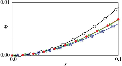
Figure 2. Comparison of the numerical and asymptotic
. Here,
. Black (filled circle): numerical solution, Red (double circle): asymptotic estimate (28), and Blu (circle): asymptotic estimate (26).
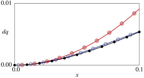
Figure 3. Comparison of the numerical and asymptotic
. Here,
. Black (filled circle): numerical solution, Red (double circle): asymptotic estimate (28), and Blu (circle): asymptotic estimate (26).
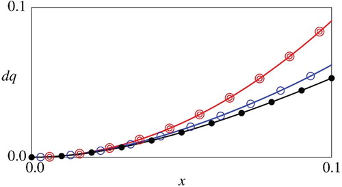
Figure 4. Comparison of the numerical and asymptotic
. Here,
. Black (filled circle): numerical solution, Red (double circle): asymptotic estimate (28), and Blu (circle): asymptotic estimate (26).
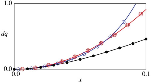
Figure for the value function demonstrates that the asymptotic estimate is reasonably accurate for sufficiently small
and captures the convex nature of the numerical solutions. As stated above, the asymptotic estimate (25) does not depend on
. Figure demonstrates that this property is reasonably satisfied for the numerical solutions with the different values of
, especially for sufficiently small
, indicating a qualitative consistency between the asymptotic and numerical results. For the optimal control
, the computational results in Figures suggest that the polynomial estimate (28) is more close to the numerical results for all
when
is small, implying that the second term of (28) truly works as a correction term to the monomial estimate (26). As visually seen in Figures , relative error between the numerical and asymptotic estimates are smaller for larger weighting coefficient
, suggesting that the asymptotic estimates are more accurate for the problem with the decision-maker having more concern with minimization of the deviation of the control from the target. Overall, the computational results demonstrate that the asymptotic estimates for small
in Proposition 2.4 are qualitatively correct for small
.
4.3. Parameter dependence of the optimal control
The HJB equation (23) is numerically solved for a variety of parameter values, so that behaviour of the optimal control , the quantity to be found through solving the optimization problem, is explored more in detail. Figures show the computed
for different values of
in the carrying capacity,
in the decay term,
in the jump term, and
and
in the performance index.
Figure 5. Comparison of for
. The relationship
is maintained in all the cases plotted in this figure.
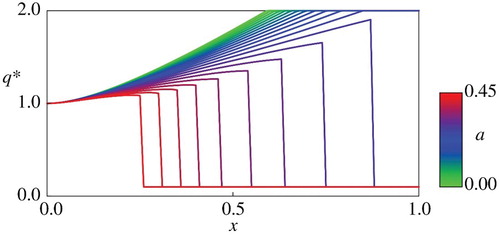
Figure 6. Comparison of for
.
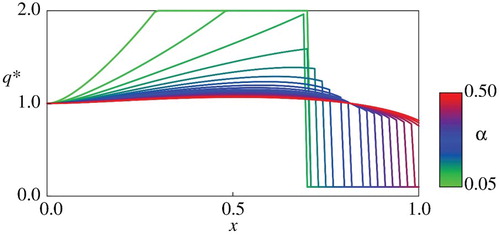
Figure 7. Comparison of for
.
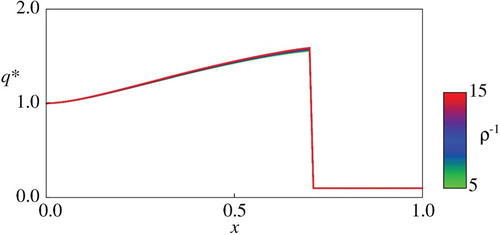
Figure 8. Comparison of for
.
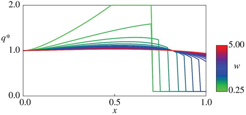
Figure 9. Comparison of for
.
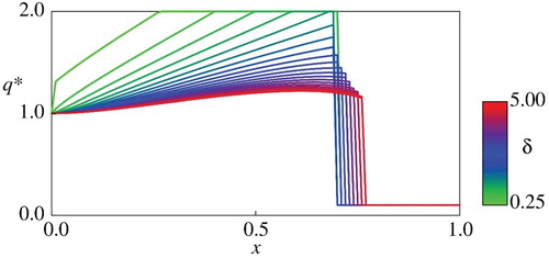
Figure for indicates qualitatively different profiles of
between small
and large
. For the smallest
,
is continuous and increasing with respect to the population
and it saturates at a point in
and equals
for larger
. The same applies to relatively small
. However, for larger
, there exists a subdomain near
such that
is optimal and
is discontinuous at the left boundary of this sub-domain. This type of discontinuous optimal control has not been found in similar stochastic control models with constant
[Citation63,Citation65]. This sudden decrease of
is considered to be due to the functional form
of the carrying capacity that depends on the control
. On the one hand, the population decays with the decay rate proportional to the control
. On the other hand, higher population abundance is possibly achieved for larger value of
if there is no decay, which is more significant for larger
. The computational results suggest that the control should be minimum, even if it deviates from the target value
, if the population
is large and its carrying capacity is a highly increasing function of the control
. From a view point of management of river environment focusing on the harmful benthic algae, the computational result for large
suggest that the flow speed should be close to the target value when the population
is small, should be maximum if
is moderate, and should be minimum if
is large. For the last case, the flow speed should be set smallest as possible in the admissible range
. This type of the control policy may not be feasible in practice for river environment where too low flow speed (or low flow discharge) triggers secondary issues like contractions of floodplains serving as habitats of many aquatic species [Citation24,Citation57]. Nevertheless, the policy can become feasible if the population is maintained small through voluntary human interventions like cleaning up of the river [Citation62]. The discontinuities appearing in
suggest that the model parameter should be carefully calibrated especially when the population is not small. The computational results in Figures provide insights into the impacts of the other model parameters on the optimal control
.
Figures and for and
show that the magnitude of the deviation
can be made smaller if larger values of the parameters are achieved at least for not large
. For the benthic algae management in rivers, the parameter
can be made larger through increasing sediment size and sediment content in river flows [Citation35,Citation54], which can be possible through sediment injection into upstream of the river reach where the benthic algae are blooming [Citation66]. Figure implies that increasing the parameter
, which is an inverse of the non-dimensional mean waiting time between floods, does not critically affect
. This is considered due to the fact that the jump discontinuously decreases the population as (4), but its influence is not persistent since it is not time-continuous.
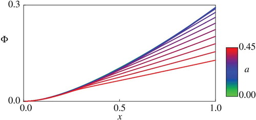
Figures and for and
exhibit the impacts of the performance index on the optimal control
. The result in Figure for not large
on the weighting coefficient
is in accordance with the intuition that the deviation
is smaller for larger value of
. Figure gives a linkage between the perspective of the decision-maker and the optimal control
. According to the computational result, the decision-maker with longer management viewpoint (smaller
) allows the deviation to become a larger
except for large
. Qualitatively similar results have been obtained in the asymptotic estimate in Proposition 2.5, again showing consistency between the asymptotic and numerical results. The sub-domain where
is optimal is narrower for larger
. The above-mentioned results on the optimal control
exploited from Figure suggest that managing the algae population dynamics with smaller deviation
requires some shorter-term perspective, such that the decision-maker tries to rapidly manage river environment.
Finally, Figure plots the computed value function for different values of
in the carrying capacity, implying that
is strictly increasing and smooth. This computational result indicates that there exist at most a countable number of optimal controls at each point, based on the discussion made just above Remark 2.4.
Figure 10. Comparison of for
. The relationship
is maintained in all the cases plotted in this figure.
5. Conclusions
This paper formulated a simplified stochastic optimization problem for logistic population dynamics with a control-dependent carrying capacity. Solving the optimization problem was ultimately reduced to finding the unique viscosity solution to the HJB equation. Solving the HJB equation was carried out with a stable finite difference scheme since the solution is not an analytical solution. Numerical solutions reasonably agreed with the asymptotic estimates. Numerical computation of the HJB equation focusing on algae population management revealed strong dependence of the optimal control on the environmental parameters. It was demonstrated that the continuity of the optimal control with respect to the state variable is critically affected by the parameter values, suggesting that they should be carefully calibrated depending on environmental conditions.
In summary, this paper formulated and explored behaviour of the minimum model for the population dynamics with an emphasis on the benthic algae population management in river environment. Although the presented results only concern the simplified model, they are useful for extended problems where controlling some population dynamics plays a central role. For example, the model can be directly incorporated into the operational model for environmental management [Citation63,Citation68]. The present model can also be used as a sub-model for describing predator-prey dynamics arising in inland fisheries management [Citation58]. A more realistic model would involve the delay [Citation7] and spatial-dependence [Citation13,Citation25] and can be numerically simulated with some algorithms, but their mathematical analysis would require more sophisticated techniques like functional analysis for infinite-dimensional dynamical systems. Handling seasonal algae population dynamics is another interesting and practically important problem. The resulting HJB equation for the seasonal-dependent problem is expected to be a time-dependent, parabolic counterpart of the one that focused on in this paper. The established finite difference scheme can be directly extended to discretization of the HJB equation in the advanced problem, which is currently undergoing. Hydraulic and hydrological observations for a more realistic mathematical modelling of the benthic algae population dynamics are undergoing as well.
Acknowledgements
The author thanks the two reviewers for their valuable comments and suggestions.
Disclosure statement
No potential conflict of interest was reported by the author.
ORCID
Hidekazu Yoshioka http://orcid.org/0000-0002-5293-3246
Additional information
Funding
References
- Y. Achdou, G.J. Buera, J.M. Lasry, P.L. Lions, and B. Moll, Partial differential equation models in macroeconomics, Phil. Trans. R. Soc. A 372 (2014), 20130397. doi: 10.1098/rsta.2013.0397
- A. Alla, M. Falcone, and D. Kalise, An efficient policy iteration algorithm for dynamic programming equations, SIAM J. Sci. Comput. 37 (2015), pp. A181–A200. doi: 10.1137/130932284
- E.J. Allen, Derivation of stochastic partial differential equations for size-and age-structured populations, J. Biol. Dyn. 3 (2009), pp. 73–86. doi: 10.1080/17513750802162754
- C. Anderson, Z. Jovanoski, H.S. Sidhu, and I.N. Towers, Logistic equation is a simple stochastic carrying capacity, ANZIAM J. 56 (2016), pp. 431–445. doi: 10.21914/anziamj.v56i0.9386
- P. Azimzadeh, Impulse Control in Finance: Numerical Methods and Viscosity Solutions, 2017. arXiv preprint arXiv:1712.01647.
- N. Bacaër, On the stochastic SIS epidemic model in a periodic environment, J. Math. Biol. 71 (2015), pp. 491–511. doi: 10.1007/s00285-014-0828-1
- F. Bai, K.E. Huff, L.J. Allen, The effect of delay in viral production in within-host models during early infection. J. Biol. Dyn (in press). Available at https://www.tandfonline.com/doi/pdf/10.1080/17513758.2018.1498984?needAccess=true.
- G. Barles and P.E. Souganidis, Convergence of approximation schemes for fully nonlinear second order equations, Asympt. Anal. 4 (1991), pp. 271–283.
- N. Bäuerle, U. Rieder, Markov Decision Processes with Applications to Finance, Springer Science & Business Media, Heidelberg, 2011
- B. Bian, M. Dai, L. Jiang, Q. Zhang, and Y. Zhong, Optimal decision for selling an illiquid stock, J. Opt. Theor. Appl. 151 (2011), pp. 402–417. doi: 10.1007/s10957-011-9897-0
- F. Brauer and C. Castillo-Chavez, Mathematical Models in Population Biology and Epidemiology, Springer, New York, 2012.
- L. Bretschger and A. Vinogradova, Best policy response to environmental shocks: Applying a stochastic framework, J. Environ. Econ. Manage (in press). Available at https://www.sciencedirect.com/science/article/pii/S0095069616302893.
- R. S. Cantrell, C. Cosner, and X. Yu, Dynamics of populations with individual variation in dispersal on bounded domains, J. Biol, Dyn. 12 (2018), pp. 288–317. doi: 10.1080/17513758.2018.1445305
- L. Chen, L. Qian, Y. Shen, and W. Wang, Constrained investment–reinsurance optimization with regime switching under variance premium principle, Insurance Math. Econ. 71 (2016), pp. 253–267. doi: 10.1016/j.insmatheco.2016.09.009
- X. Chen, W. Wang, D. Ding, and S.L. Lei, A fast preconditioned policy iteration method for solving the tempered fractional HJB equation governing American options valuation, Comput. Math. Appl. 73 (2017), pp. 1932–1944. doi: 10.1016/j.camwa.2017.02.040
- M.G. Crandall, H. Ishii, and P.L. Lions, User’s guide to viscosity solutions of second order partial differential equations, Bull. Am. Math. Soc. 27 (1992), pp. 1–67. doi: 10.1090/S0273-0979-1992-00266-5
- D.M. Dang and P.A. Forsyth, Better than pre-commitment mean-variance portfolio allocation strategies: A semi-self-financing Hamilton–Jacobi–Bellman equation approach, Euro. J. Oper. Res. 250 (2016), pp. 827–841. doi: 10.1016/j.ejor.2015.10.015
- F.A. Dorini, M.S. Cecconello, and L.B. Dorini, On the logistic equation subject to uncertainties in the environmental carrying capacity and initial population density, Commun. Nonlinear Sci. Numer. Simul. 33 (2016), pp. 160–173. doi: 10.1016/j.cnsns.2015.09.009
- L. Doyen, C. Béné, M. Bertignac, L.R. Little, C. Macher, D.J. Mills, A. Noussair, S. Pascoe, J.-C. Pereau, N. Sanz, A.-M. Schwarz, T. Smith, O. Thébaud, Ecoviability for ecosystem-based fisheries management. Fish Fisher 18 (2017), pp. 1056–1072 doi: 10.1111/faf.12224
- T.J. Entwisle, Phenology of the Cladophora-Stigeoclonium community in two urban creeks of Melbourne, Austral. J. Marine Freshwater Res. 40 (1989), pp. 471–489. doi: 10.1071/MF9890471
- W.H. Fleming, H.M. Soner, Controlled Markov Processes and Viscosity Solutions, Springer Science & Business Media, New York, 2006
- O. Fovet, G. Belaud, X. Litrico, S. Charpentier, C. Bertrand, P. Dollet, C. Hugodot, A model for fixed algae management in open channels using flushing flows. River Res. Appl 28 (2012), pp. 960–972 doi: 10.1002/rra.1495
- T.B. Gyulov and R.L. Valkov, American option pricing problem transformed on finite interval, Int. J. Comput. Math. 93 (2016), pp. 821–836. doi: 10.1080/00207160.2014.906587
- L. Hansen and T.J. Sargent, Robust control and model uncertainty, Am. Econ. Rev. 91 (2001), pp. 60–66. doi: 10.1257/aer.91.2.60
- E.E. Holmes, M.A. Lewis, J.E. Banks, and R.R. Veit, Partial differential equations in ecology: Spatial interactions and population dynamics, Ecology 75 (1994), pp. 17–29. doi: 10.2307/1939378
- A. Hussner, Management and control methods of invasive alien freshwater aquatic plants: A review, Aqua. Bot. 136 (2017), pp. 112–137. doi: 10.1016/j.aquabot.2016.08.002
- R. Inui, Y. Akamatsu, and Y. Kakenami, Quantification of cover degree of alien aquatic weeds and environmental conditions affecting the growth of Egeria densa in Saba River, Japan. J. JSCE. 72 (2016), pp. I_1123–I_1128 (in Japanese with English Abstract). doi: 10.2208/jscejhe.72.I_1123
- N. Jafari, A Phillips, P.M. Pardalos, A robust optimization model for an invasive species management problem. Environ. Model. Assess. 23(6) (2018), pp. 743–752 doi: 10.1007/s10666-018-9631-5
- S. Koike, A Beginner’s Guide to the Theory of Viscosity Solutions, Mathematical Society of Japan, Tokyo, 2014.
- J. Kurihara, M. Michinaka, and Y. Akamatsu, Factor analysys of luxuriant growth and suppression of Egeria densa in Gonokawa River, Japan. Adv. River Eng. 24 (2018), pp. 297–302.
- R. Lande, S. Engen, and B.E. Saether, Stochastic Population Dynamics in Ecology and Conservation, Oxford University Press on Demand, Oxford, 2003.
- X. Litrico, V. Fromion, Modeling and Control of Hydrosystems, Springer Science & Business Media, London, 2009
- M. Liu and C. Bai, Optimal harvesting of a stochastic mutualism model with Lévy jumps, Appl. Math. Comput. 276 (2016), pp. 301–309.
- G. Lobera, L. Muñoz, J.A. López-Tarazón, D. Vericat, and R.J. Batalla, Effects of flow regulation on river bed dynamics and invertebrate communities in a Mediterranean river, Hydrobiologia 784 (2017), pp. 283–304. doi: 10.1007/s10750-016-2884-6
- J.J. Luce, M.F. Lapointe, A.G. Roy, and D.B. Ketterling, The effects of sand abrasion of a predominantly stable stream bed on periphyton biomass losses, Ecohydrology 6 (2013), pp. 689–699. doi: 10.1002/eco.1332
- E. Lungu and B. Øksendal, Optimal harvesting from a population in a stochastic crowded environment, Msth. Biosci. 145 (1997), pp. 47–75. doi: 10.1016/S0025-5564(97)00029-1
- J. Lv, K. Wang, and J. Jiao, Stability of stochastic Richards growth model, Appl. Math. Model. 39 (2015), pp. 4821–4827. doi: 10.1016/j.apm.2015.04.016
- P.S. Mandal, L.J. Allen, and M. Banerjee, Stochastic modeling of phytoplankton allelopathy, Appl. Math. Model. 38 (2014), pp. 1583–1596. doi: 10.1016/j.apm.2013.08.031
- Y. Mau, X. Feng, and A. Porporato, Multiplicative jump processes and applications to leaching of salt and contaminants in the soil, Phys. Rev. E 90 (2014), 052128. doi: 10.1103/PhysRevE.90.052128
- M. Neilan, A.J. Salgado, and W. Zhang, Numerical analysis of strongly nonlinear PDEs, Acta Numer. 26 (2017), pp. 137–303. doi: 10.1017/S0962492917000071
- A.J. Neverman, R.G. Death, I.C. Fuller, R. Singh, and J.N. Procter, Towards mechanistic hydrological limits: A literature synthesis to improve the study of direct linkages between sediment transport and periphyton accrual in gravel-bed rivers, Environ. Manage. 62 (2018), pp. 740–755. doi: 10.1007/s00267-018-1070-1
- B. Øksendal, Stochastic Differential Equations, Springer, Berlin, Heidelberg, 2003.
- B. Øksendal and A. Sulem, Applied Stochastic Control of Jump Diffusions, Springer, Berlin, 2005.
- R.J. Plemmons, M-matrix characterizations. I. Nonsingular M-matrices, Linear Algebra Appl. 18 (1977), pp. 175–188. doi: 10.1016/0024-3795(77)90073-8
- C. Reisinger and P.A. Forsyth, Piecewise constant policy approximations to Hamilton–Jacobi–Bellman equations, Appl. Numer. Math. 103 (2016), pp. 27–47. doi: 10.1016/j.apnum.2016.01.001
- F. Santambrogio, Optimal Transport for Applied Mathematicians, Birkäuser, New York, 2015.
- M.J. Santos, L.W. Anderson, and S.L. Ustin, Effects of invasive species on plant communities: An example using submersed aquatic plants at the regional scale, Biol. Invasions. 13 (2011), pp. 443–457. doi: 10.1007/s10530-010-9840-6
- L. Sanz and J.A. Alonso, Approximate reduction of linear population models governed by stochastic differential equations: Application to multiregional models, J. Biol. Dyn. 11 (2017), pp. 461–479. doi: 10.1080/17513758.2017.1380852
- H. Schurz, Modeling, analysis and discretization of stochastic logistic equations, Int. J. Numer. Anal. Model. 4 (2007), pp. 178–197.
- P.D.N. Srinivasu, D.K.K. Vamsi, and V.S. Ananth, Additional food supplements as a tool for biological conservation of predator-prey systems involving type III functional response: A qualitative and quantitative investigation, J. Theor. Biol. 455 (2018), pp. 303–318. doi: 10.1016/j.jtbi.2018.07.019
- G. Thiébaut, M. Gillard, and C. Deleu, Growth, regeneration and colonisation of Egeria densa fragments: The effect of autumn temperature increases, Aqua. Ecol. 50 (2016), pp. 175–185. doi: 10.1007/s10452-016-9566-3
- H.R. Thieme, Mathematics in Population Biology, Princeton University Press, Princeton and Oxford, 2018.
- L.H. Thomas, Elliptic Problems in Linear Difference Equations Over a Network, Watson Sci. Comp. Lab. Rep, Columbia University, New York, 1949.
- T. Tsujimoto and T. Tashiro, Application of population dynamics modeling to habitat evaluation-growth of some species of attached algae and its detachment by transported sediment, Hydroécol. Appl. 14 (2004), pp. 161–174. doi: 10.1051/hydro:2004010
- U.R.S. Uehlinger, H. Bührer, and P. Reichert, Periphyton dynamics in a floodprone prealpine river: Evaluation of significant processes by modelling, Freshw. Biol. 36 (1996), pp. 249–263. doi: 10.1046/j.1365-2427.1996.00082.x
- H. Wang, Y. Li, J. Li, R. An, L. Zhang, M. Chen, Influences of hydrodynamic conditions on the biomass of benthic diatoms in a natural stream. Ecol. Indic 92 (2018), pp. 51–60 doi: 10.1016/j.ecolind.2017.05.061
- S. Wang, S. Zhang, and Z. Fang, A superconvergent fitted finite volume method for Black–Scholes equations governing European and American option valuation, Numer. Methods Partial Differ. Equ. 31 (2015), pp. 1190–1208. doi: 10.1002/num.21941
- Y. Yaegashi, H. Yoshioka, K. Unami, and M. Fujihara, An optimal management strategy for stochastic population dynamics of released Plecoglossus altivelis in rivers, Int. J. Model. Simul. Sci. Comput. 8 (2017), 16pp: 1750039. doi: 10.1142/S1793962317500398
- Y. Yaegashi and H. Yoshioka, Unique solvability of a singular stochastic control model for population management, Syst. Control Lett. 116 (2018), pp. 66–70. doi: 10.1016/j.sysconle.2018.03.009
- Y. Yaegashi, H. Yoshioka, K. Unami, and M. Fujihara, A singular stochastic control model for sustainable population management of the fish-eating waterfowl Phalacrocorax carbo, J. Environ. Manage. 219 (2018), pp. 18–27. doi: 10.1016/j.jenvman.2018.04.099
- B.C. Yen, Open channel flow resistance, J. Hydraul. Eng. 128 (2002), pp. 20–39. doi: 10.1061/(ASCE)0733-9429(2002)128:1(20)
- H. Yoshioka, ‘Mathematical exercise’ on a solvable stochastic control model for animal migration, ANZIAM J. 59 (2018), pp. 15–28. doi: 10.21914/anziamj.v59i0.12566
- H. Yoshioka and Y. Yaegashi, Singular stochastic control model for algae growth management in dam downstream, J. Biol. Dyn. 12 (2018), pp. 242–270. doi: 10.1080/17513758.2018.1436197
- H. Yoshioka and Y. Yaegashi, Robust stochastic control modeling of dam discharge to suppress overgrowth of downstream harmful algae, Appl. Stoch. Model. Bus. 34 (2018), pp. 338–354. doi: 10.1002/asmb.2301
- H. Yoshioka and Y. Yaegashi, A finite difference scheme for variational inequalities arising in stochastic control problems with several singular control variables, Math. Comput. Simul. 156 (2019), pp. 40–66. doi: 10.1016/j.matcom.2018.06.013
- H. Yoshioka, Y. Yaegashi, Y. Yoshioka, K. Hamagami, and M. Fujihara, Wise-use of sediment for river restoration: Numerical approach via HJBQVI, Commun. Comput. Inf. Sci. 946 (2018), pp. 451–465.
- H. Yoshioka, T. Shirai, and D. Tagami, A mixed optimal control approach for upstream fish migration, J. Sust. Dev. Energy Water Environ. 7 (2019), pp. 101–121. doi: 10.13044/j.sdewes.d6.0221
- H. Yoshioka, Y. Yaegashi, Y. Yoshioka, and K. Hamagami, Hamilton–Jacobi–Bellman quasi-variational inequality arising in an environmental problem and its numerical discretization, Comput. Math. Appl. ( Accepted on December 1, 2018, in press). Available at https://www.sciencedirect.com/science/article/pii/S0898122118306965
- W. Yuan, S. Lai, and H. Hu, Optimal consumption analysis for a stochastic growth model with technological shocks, Appl. Stoch. Model. Bus. 34 (2018), pp. 746–755. doi: 10.1002/asmb.2384
- S. Zulkifly, et al., The epiphytic microbiota of the globally widespread macroalga Cladophora glomerata (Chlorophyta, Cladophorales), Am. J. Bot. 99 (2012), pp. 1541–1552. doi: 10.3732/ajb.1200161
Appendix
Proofs of the propositions stated in the main text are provided in this appendix.
Proof of Proposition 2.1
The proof here is just an application of Theorem 9.8 in Øksendal and Sulem [Citation43], since the SDE (3) admits a path-wise unique solution confined in , and then the continuity of the value function
in
follows from the Lipschitz continuity of
in
. The fact that
is a viscosity solution follows from the argument essentially similar to that of the proof for Theorem 9.8 in Øksendal and Sulem [Citation43] combined with the fact that
(
) if
.
Proof of Proposition 2.2
The proof here is based on a standard technique employed with the variable-doubling of the comparison theorems [Citation16,Citation29], but employs a special auxiliary function to deal with the issue of not enforcing boundary conditions at , where the HJB equation (9) is directly solved.
By the positivity of ,
, and
in
, there exists a constant
close to
such that
(A1)
(A1) for any
because
(A2)
(A2) for any
. Choose such a
. Set
(A3)
(A3) which is a smooth, non-negative, increasing, and convex function.
Suppose that is a viscosity sub-solution. We construct a new viscosity sub-solution from
. Set
(A4)
(A4) with a constant
. Then,
with
is also a viscosity sub-solution. In fact, if
then
. By (12), for any
, we have
(A5)
(A5) for any test functions
satisfying the conditions in Definition 2.1(a). The relationship
(A6)
(A6) shows
(A7)
(A7) Set
(A8)
(A8) which is an increasing function with respect to
for each
. In addition, for
and
, we have
(A9)
(A9) since
. The function
is smooth, non-negative, increasing, and
(A10)
(A10) By (A10), we have
(A11)
(A11) By (A7) and (A11), we further have
(A12)
(A12) implying that
is a viscosity sub-solution.
Now, we claim a comparison theorem: for any viscosity sub-solution and viscosity-super solution
such that
,
in
. The following part of the proof is based on a contradiction argument. For any
,
, set
(A13)
(A13) as in the standard variable-doubling technique (Theorem 3.7 of Koike [Citation29], Theorem 8.2 of Crandall et al. [Citation16]). Assume
at some
. By the assumption, we have
. Without loss of generality, assume
. Otherwise, we have nothing to prove. Choose sufficiently small
such that
.
Let be the maximizer of
in
. Then, as in the standard argument of comparison theorems, we can choose a sub-sequence of
such that
(A14)
(A14)
(A15)
(A15) and
(A16)
(A16) By the assumption of
at
and the fact that
diverges to
at
, we must have
. Assuming
is small, we can choose
such that
, which is hereafter assumed.
By the above argument and Definition 2.1, the functions
(A17)
(A17) and
(A18)
(A18) are test functions for viscosity sub- and super- solutions
and
, respectively. Therefore, we have
(A19)
(A19) and
(A20)
(A20) We then arrive at
(A21)
(A21) which is rewritten as
(A22)
(A22) By the definition of
, we obtain
(A23)
(A23) Substituting (A23) into (A22) yields
(A24)
(A24) Because
is Lipschitz continuous with respect to
and
, taking the limit
in (A24) yields
(A25)
(A25) This is a contradiction since
.
Uniqueness of viscosity solutions immediately follows from the above-presented comparison argument and their continuity. This is because a viscosity solution is continuous in and it is a viscosity sub-solution as well as a viscosity super-solution.
Proof of Proposition 2.4
By the assumption, for small , the HJB equation (23) reduces to
(A26)
(A26) Assuming the asymptotic form
with some
and
, substituting this into (A26) yields
(A27)
(A27) Now, we have
(A28)
(A28) Substituting (A28) into (A27) yields
(A29)
(A29) Matching the coefficients in both-hand sides of (A29) yields
and thus
, implying
, which gives (25).
For the asymptotic estimate of , we use (25). By the definition, we have
(A30)
(A30) Substituting (25) into (A30) yields
(A31)
(A31) Then, a simple differentiation gives
(A32)
(A32) which can be rewritten as
(A33)
(A33) The equality (A33) shows
as
. Therefore, we can use the expansion
(A34)
(A34) Then, (A33) and (A34) gives
(A35)
(A35) and thus
(A36)
(A36) leading to (26).
Proof of Proposition 3.1
The proof here is essentially the same with but simpler than that in Chapters 3 and 4 of Azimzadeh [Citation5] since the present HJB equation does not involve the nonlinear non-local term. To prove the convergence, we show the monotonicity, stability, and consistency of the scheme. Monotonicity of the scheme follows from the fact that the matrix is an M-matrix. Consistency of the scheme is straightforwardly proven just following Lemma 4.3.16 of Azimzadeh [Citation5].
Stability of the scheme, namely uniform boundedness of numerical solutions independent from the discretization parameter , is proven as follows. Set
. Assume that the maximum is achieved at some
such that
. Then, by (41), we have
(A37)
(A37) which leads to
(A38)
(A38) and
(A39)
(A39)
Combining (A38) and (A39) yields
(A40)
(A40) Since
(A41)
(A41) substituting (A41) into (A40) yields
(A42)
(A42) showing the stability. If
, then an essentially similar argument again leads to (A42). If
, then the stability is trivial.
In summary, the scheme is monotone, consistent, and stable. Therefore, a straightforward application of the convergence theorem (Barles and Souganidis [Citation8], Theorem 4.3.19 of Azimzadeh [Citation5]) combined with Proposition 2.2 leads to the convergence of the scheme.