Dynamical analysis of an integrated pest management predator–prey model with weak Allee effect

Abstract

In this paper, a pest management predator–prey model with weak Allee effect on predator and state feedback impulsive control on prey is introduced and analysed, where the yield of predator released and intensity of pesticide sprayed are assumed to be linearly dependent on the selected pest control level. For the proposed model, the existence and stability of the order-1 periodic orbit of the control system are discussed. Meanwhile, with the aim of minimizing the input cost in practice, an optimization model is constructed to determine the optimal quantity of the predator released and the intensity of pesticide sprayed. The theoretical results and numerical simulations indicated that the number of pests can be limited to below an economic threshold and displays periodic variation under the proposed control strategy. In addition, it indicated in numerical simulations that an order-2 periodic orbit exists for some certain parameters.

Keywords:

• Integrated pest management
• impulsive state feedback control
• order-k periodic solution
• stability
• weak Allee effect

1. Introduction

Food losses due to pests and plant diseases are nowadays one of the major threats to food security, particularly in large parts of the developing world. As reported by the United Nations, the world population in 2014 was estimated at 7.2 billion, with an approximate yearly growth of 82 million, a quarter of which occurs in the least developed countries [35]. This unprecedented amount of people in the world poses serious challenges for food producers and policy-makers, specially regarding the minimization of crop losses due to pests and plant diseases, which have been estimated to be as high as 40% of the world production [22]. This issue has been a matter of active research for many decades, where the main challenge lies in the unavoidable trade-off between pest reduction, financial costs, effects on human health and environmental impact. Spraying chemical pesticide can kill part of the agricultural pests and control the rapid growth of pests, however, the extensive use and unreasonable abuse of pesticides destroy the structure of the agricultural ecosystem, reduce biodiversity, and lead to the residue of chemical composition in crops, threatening the health of human beings. In addition, the long-term use of pesticides also leads to pest resistance, weakens or reduces the ability of natural enemy to control pests, results in frequent and even more rampant pests, which falls into the vicious cycle that it is the more drug treatment the more difficult to govern. A large number of facts show that the side effects of chemical pesticides have challenged the single method of pest control by chemical pesticides. In fact, natural enemies of the agricultural pests also play an important role in control the quantity pests [3,10,19,36]. Therefore, the problem of pest control has necessarily to be addressed in an integrated manner, which has motivated the development of various integrated approaches, such as Integrated Pest Management (IPM) [2,22,37].

IPM's basic principle consists in the judicious and coordinated use of multiple pest control mechanisms (e.g. biological control, cultural practices, selected chemical methods, etc.) in ways that complement one another, maintaining pest damage below acceptable economic levels, while minimizing hazards to humans, animals, plants and the environment. IPM has been proved to be more effective than the classic methods both experimentally [36,38] and theoretically [31,41]. The key concept for the implementation of a pest control programme in an IPM framework is that of economic injury level, which means the lowest pest population density that will cause economic damage. In general, it is assumed that a number of pest control mechanisms is available, for instance biological methods, cultural practices, natural enemies, habitat management, synthetic pesticides, etc. The basic decision rules rely on a predefined economic injury level and an economic threshold, which gives the pest population density above which control actions must be taken so as to prevent the pest population from reaching the economic injury level. An IPM-based pest control scheme, in its simplest form, will then require that whenever the amount of pests is less than the economic threshold only ecologically benign control measures are applied, i.e. those that enhance natural control. If natural control is not capable of preventing the pest population from reaching the economic injury level, then synthetic pesticides come into play, nevertheless, in adequate combination with environmentally friendly control measures so as to minimize the amount of pesticides released into the underlying ecosystem. In practice, however, to develop and implement an IPM-based pest control programme sustainable both in ecological and economic terms is by no means trivial tasks.

Integrated pest management may cause a radical change in biological population due to the variety of manual intervention. This phenomenon also occurs in many dynamical systems due to abrupt changes at certain instants during the evolution process. To describe these phenomena in mathematics, impulsive differential equations are a powerful tool. The research on the theory of impulsive state feedback control dynamic systems (ISFCDS) has made a great progress in recent years, and the basic theory of impulsive semi-dynamical systems, as well as the criteria for checking the existence and stability of periodic solutions of impulsive semi-dynamical systems are presented [4–6,8,9]. Besides the theoretical study aspect of impulsive semi-dynamical systems, in application aspect, Tang et al. made a pioneer work in pest management predator–prey model with state-dependent impulse [28,29,32]. Since then many scholars have introduced ISFCDS in predator–prey system to model the pest control action [12–14,20,23,26,27,30,33,39,42,43,46,47]. Among these studies, Jiao et al. investigated the Allee effect on a single population model with state-dependent impulsively unilateral diffusion [14]. The Allee effect is a phenomenon in biology characterized by a correlation between population size or density and the mean individual fitness (often measured as per capita population growth rate) of a population or species [11,15,17]. Many scholars investigated the rich dynamical behaviours of predator–prey model with Allee effect [1,7,16,18,21,24,34,40,44,45,48]. To consider that the predators are difficult to seek spouses when the species has a low population density, the Allee effect on predator is introduced to model phenomenon. Thus in this work, an integrated pest management predator–prey model with Allee effect is presented by introducing the biological control threshold and the chemical control threshold, where the pest control level is selected between the two control thresholds.

The rest of the paper is organized as follows. In Section 2, the mathematical model is formulated and some preliminaries are presented. The dynamic properties of the free system are introduced in Section 3, and then followed by the control system including the existence and stability of the order-1 periodic orbit. Existence depends on the method of successive functions, and stability is by the limit method of successor point sequences and analogue of Poincaré criterion. What't more, an optimization problem is formulated to minimize the total cost in the pest control. In Section 4, the numerical simulations are carried out to verify the theoretical results. And a brief conclusion is presented in Section 5.

2. Model formulation and preliminaries

2.1. Mathematical model

Let $x\left(t\right)$ and $y\left(t\right)$ denote the population of the pest and the predator at time t, respectively. The intrinsic rate of increase of the pest is assumed to follow the Logistic type, i.e. $r(1-x\left(t\right)/K)$, where r is the birth rate, K is the environmental carrying capacity for the pest in absent of predator. For the species without environmental carrying capacity constraint, K can be chosen as a larger positive constant. The restriction from the predator is proportion to the pest, i.e. $bx\left(t\right)y\left(t\right)$. The conversion rate of predators after predating pests is similar to weak Allee effect, i.e. $y\left(t\right)/y\left(t\right)+m$, where m is Allee effect constant. And d is the death rate of predator. The model can be formulated as follows: (1) $\begin{array}{rl}& \frac{\mathrm{d}x\left(t\right)}{\mathrm{d}t}=rx\left(t\right)\left(1-\frac{x\left(t\right)}{K}\right)-bx\left(t\right)y\left(t\right),\\ & \frac{\mathrm{d}y\left(t\right)}{\mathrm{d}t}=cx\left(t\right)y\left(t\right)\frac{y\left(t\right)}{y\left(t\right)+m}-\mathrm{d}y\left(t\right).\end{array}$(1) Considering the harm of the pest on crops, let $x_{ZX}$ denote the pest slight harmful threshold (or biological control level) and $x_{ZD}(x_{ZX}<x_{ZD}<K)$ denote the pest economic injury threshold (or chemical control level). To achieve the control effect, assume that the yield releases of the predator at $x_{ZX}$ and $x_{ZD}$ are ${\tau }_{max}$ and ${\tau }_{min}({\tau }_{max}>{\tau }_{min}\ge 0),$ respectively. Suppose that the chemical control strength at $x_{ZD}$ is $p_{max}$ to the pest and $q_{max}$ to the predator. To determine the optimal control threshold, an integrated pest control threshold $x_T$ is assumed to be between $x_{ZX}$ and $x_{ZD}(x_{ZX}\le x_T\le x_{ZD}).$ Once the population of pests reaches control level $x_T$, The corresponding pest management strategy, a certain yield of releases of predators $\tau \left(x_T\right)$ and a certain strength of insecticide spraying $p\left(x_T\right),q\left(x_T\right)$, should be adopted. And $\tau \left(x_T\right),p\left(x_T\right),q\left(x_T\right)$ are linearly dependent on pest control level $x_T$, which are as follows: (2) $\begin{array}{rl}\tau \left(x_T\right)& ={\tau }_{max}-({\tau }_{max}-{\tau }_{min})\frac{x_T-x_{ZX}}{x_{ZD}-x_{ZX}},\\ p\left(x_T\right)& =p_{max}\frac{x_T-x_{ZX}}{x_{ZD}-x_{ZX}},\\ q\left(x_T\right)& =q_{max}\frac{x_T-x_{ZX}}{x_{ZD}-x_{ZX}}.\end{array}$(2) According to the effect of insecticide, the strength of insecticide spraying to the pest $p\left(x_T\right)$ is equal or greater than that to the predator $q\left(x_T\right).$

Based on the above control strategy, an integrated pest management predator–prey model with Allee effect is obtained in the following: (3) $\left\{\begin{array}{l}\left.\begin{array}{c}\frac{\mathrm{d}x\left(t\right)}{\mathrm{d}t}=rx\left(t\right)\left(1-\frac{x\left(t\right)}{K}\right)-bx\left(t\right)y\left(t\right),\\ \frac{\mathrm{d}y\left(t\right)}{\mathrm{d}t}=cx\left(t\right)y\left(t\right)\frac{y\left(t\right)}{y\left(t\right)+m}-\mathrm{d}y\left(t\right),\end{array}\right\}x<x_T,\\ \left.\begin{array}{c}\mathrm{\Delta }x\left(t\right)=-p\left(x_T\right)x\left(t\right)\\ \mathrm{\Delta }y\left(t\right)=-q\left(x_T\right)y\left(t\right)+\tau \left(x_T\right)\end{array}\right\}x=x_T.\end{array}\right.$(3)

2.2. Preliminaries

For the state-dependent impulsive differential equations (4) $\left\{\begin{array}{c}\left.\begin{array}{c}\frac{\mathrm{d}x}{\mathrm{d}t}=P(x,y)\\ \frac{\mathrm{d}y}{\mathrm{d}t}=Q(x,y)\end{array}\right\}\mathrm{if}\mathrm{\Phi }(x,y)\ne 0,\\ \left.\begin{array}{c}\mathrm{\Delta }x=\alpha (x,y)\\ \mathrm{\Delta }y=\beta (x,y)\end{array}\right\}\mathrm{if}\mathrm{\Phi }(x,y)=0,\end{array}\right.$(4) where $\mathrm{\Phi }(x,y)=0$ describes the states at which the control strategy is taken on, α and β describe the effects of the control strategy and $(x,y)\in \mathrm{\Omega }\subset R^2$. $P(x,y)$ and $Q(x,y)$ are arbitrarily derivative with respect to $(x,y)\in \mathrm{\Omega }$; α and β are linearly dependent on x and y, i.e. ${\mathrm{\Phi }}_x,{\mathrm{\Phi }}_y,{\alpha }_x,{\alpha }_y,{\beta }_x,{\beta }_y$ are constant, let's denote $M=\left\{\right(x,y\left)|\mathrm{\Phi }\right(x,y)=0\}$ and $N=\left\{\right(x,y)|x=x^{\mathrm{\prime }}+\alpha (x^{\mathrm{\prime }},y^{\mathrm{\prime }}),y=y^{\mathrm{\prime }}+\beta (x^{\mathrm{\prime }},y^{\mathrm{\prime }}),(x^{\mathrm{\prime }},y^{\mathrm{\prime }})\in M\}$.

Definition 2.1

Successor function [8]

Suppose that the impulse set M and the phase set N are both line. Define the coordinate in the phase set N as follows: denote the point of intersection Q between N and x-axis as O, then the coordinate of any point A in N is defined as the distance between A and Q, and denoted by a. Let C denote the point of intersection between the trajectory starting from A and the impulse set M, and B denote the phase point of C after impulse with coordinate b. Then we define B as the successor point of A, and the successor function $f_{\mathrm{sor}}$ at A is defined $f_{\mathrm{sor}}\left(A\right)=y_B-y_A=b-a$, which is also continuous on N.

Remark 1

If there exists a point $L(x_L,y_L)\in N$ such that $f_{\mathrm{sor}}\left(L\right)=0$, then the orbit starting from L forms a periodic orbit.

Assume that there exists an order-1 periodic orbit in system (2(2) $\begin{array}{rl}\tau \left(x_T\right)& ={\tau }_{max}-({\tau }_{max}-{\tau }_{min})\frac{x_T-x_{ZX}}{x_{ZD}-x_{ZX}},\\ p\left(x_T\right)& =p_{max}\frac{x_T-x_{ZX}}{x_{ZD}-x_{ZX}},\\ q\left(x_T\right)& =q_{max}\frac{x_T-x_{ZX}}{x_{ZD}-x_{ZX}}.\end{array}$(2) ), and let ${\gamma }_L=\widehat{L{L}^{-}L}$ denoted the order-1 periodic orbit starting from L, its parameter equation is denoted by $x=\phi \left(s\right)$, $y=\varphi \left(s\right)$, expressed with the arc length s starting from L, where $0\le s\le s_L$. Since the arc length s is a function, i.e. $s=s\left(t\right)$, where $0\le t\le T_L$, then the solution $x=\xi \left(t\right)\triangleq \phi \left(s\right(t\left)\right)$ and $y=\eta \left(t\right)\triangleq \varphi \left(s\right(t\left)\right)$ is a $T_L$ order-1 periodic solution.

Lemma 2.2

Stability Criterion [25,33]

The $T_L$ period-1 solution $\mathbf{x}\left(t\right)=\left(\xi \right(t),\eta (t\left)\right)$ of the model (2(2) $\begin{array}{rl}\tau \left(x_T\right)& ={\tau }_{max}-({\tau }_{max}-{\tau }_{min})\frac{x_T-x_{ZX}}{x_{ZD}-x_{ZX}},\\ p\left(x_T\right)& =p_{max}\frac{x_T-x_{ZX}}{x_{ZD}-x_{ZX}},\\ q\left(x_T\right)& =q_{max}\frac{x_T-x_{ZX}}{x_{ZD}-x_{ZX}}.\end{array}$(2) ) is orbitally asymptotically stable if the convergency ratio ${\rho }_{{\gamma }_L}$ is less than one, where $\begin{array}{rl}& {\rho }_{{\gamma }_L}\triangleq \left|\frac{f_{+}^I\left[\right(1+{\beta }_y){\mathrm{\Phi }}_x-{\beta }_x{\mathrm{\Phi }}_y]+g_{+}^I\left[\right(1+{\alpha }_x){\mathrm{\Phi }}_y-{\alpha }_y{\mathrm{\Phi }}_x]}{f^I{\mathrm{\Phi }}_x+g^I{\mathrm{\Phi }}_y}\right|\\ & \exp \left({\int }_{0^{+}}^T{\left[\frac{\mathrm{\partial }f}{\mathrm{\partial }x}+\frac{\mathrm{\partial }g}{\mathrm{\partial }y}\right]}_{\left(\xi \right(t),\eta (t\left)\right)}\right),\end{array}$$f^I\left(g^I\right)$ represents the value of $f\left(g\right)$ at $L^{-}\left(\xi \right(T_L),\eta (T_L\left)\right)\in M,$ and $f_{+}^I\left(g_{+}^I\right)$ represents the value of $f\left(g\right)$ at $L\left(\xi \right(0^{+}),\eta (0^{+}\left)\right)\in N$.

3. Dynamic properties of the control system

System (1(1) $\begin{array}{rl}& \frac{\mathrm{d}x\left(t\right)}{\mathrm{d}t}=rx\left(t\right)\left(1-\frac{x\left(t\right)}{K}\right)-bx\left(t\right)y\left(t\right),\\ & \frac{\mathrm{d}y\left(t\right)}{\mathrm{d}t}=cx\left(t\right)y\left(t\right)\frac{y\left(t\right)}{y\left(t\right)+m}-\mathrm{d}y\left(t\right).\end{array}$(1) ) is called the free system, and system (3(3) $\left\{\begin{array}{l}\left.\begin{array}{c}\frac{\mathrm{d}x\left(t\right)}{\mathrm{d}t}=rx\left(t\right)\left(1-\frac{x\left(t\right)}{K}\right)-bx\left(t\right)y\left(t\right),\\ \frac{\mathrm{d}y\left(t\right)}{\mathrm{d}t}=cx\left(t\right)y\left(t\right)\frac{y\left(t\right)}{y\left(t\right)+m}-\mathrm{d}y\left(t\right),\end{array}\right\}x<x_T,\\ \left.\begin{array}{c}\mathrm{\Delta }x\left(t\right)=-p\left(x_T\right)x\left(t\right)\\ \mathrm{\Delta }y\left(t\right)=-q\left(x_T\right)y\left(t\right)+\tau \left(x_T\right)\end{array}\right\}x=x_T.\end{array}\right.$(3) ) is called control system. In this section, the dynamic properties of the free system will be discussed firstly, and then followed by the control system.

3.1. Dynamic properties of the free system

For the free system, the following result holds:

Lemma 3.1

The solutions of system (1(1) $\begin{array}{rl}& \frac{\mathrm{d}x\left(t\right)}{\mathrm{d}t}=rx\left(t\right)\left(1-\frac{x\left(t\right)}{K}\right)-bx\left(t\right)y\left(t\right),\\ & \frac{\mathrm{d}y\left(t\right)}{\mathrm{d}t}=cx\left(t\right)y\left(t\right)\frac{y\left(t\right)}{y\left(t\right)+m}-\mathrm{d}y\left(t\right).\end{array}$(1) ) is positive and bounded.

Proof.

Let $\left(x\right(t),y(t\left)\right)$ be a solution of system (1(1) $\begin{array}{rl}& \frac{\mathrm{d}x\left(t\right)}{\mathrm{d}t}=rx\left(t\right)\left(1-\frac{x\left(t\right)}{K}\right)-bx\left(t\right)y\left(t\right),\\ & \frac{\mathrm{d}y\left(t\right)}{\mathrm{d}t}=cx\left(t\right)y\left(t\right)\frac{y\left(t\right)}{y\left(t\right)+m}-\mathrm{d}y\left(t\right).\end{array}$(1) ) with the initial condition $\left(x\right(0)>0,y(0)>0)$, by the equations of system (1(1) $\begin{array}{rl}& \frac{\mathrm{d}x\left(t\right)}{\mathrm{d}t}=rx\left(t\right)\left(1-\frac{x\left(t\right)}{K}\right)-bx\left(t\right)y\left(t\right),\\ & \frac{\mathrm{d}y\left(t\right)}{\mathrm{d}t}=cx\left(t\right)y\left(t\right)\frac{y\left(t\right)}{y\left(t\right)+m}-\mathrm{d}y\left(t\right).\end{array}$(1) ), there is $\begin{array}{rl}x\left(t\right)& =x\left(0\right)\exp \left\{{\int }_0^t\left(r-\frac{rx\left(s\right)}{K}-by\left(s\right)\right)\mathrm{d}s\right\}>0,\\ y\left(t\right)& =y\left(0\right)\exp \left\{{\int }_0^t\left(\frac{cx\left(s\right)y\left(s\right)}{y\left(s\right)+m}-d\right)\mathrm{d}s\right\}>0.\end{array}$ Thus the solutions of system (1(1) $\begin{array}{rl}& \frac{\mathrm{d}x\left(t\right)}{\mathrm{d}t}=rx\left(t\right)\left(1-\frac{x\left(t\right)}{K}\right)-bx\left(t\right)y\left(t\right),\\ & \frac{\mathrm{d}y\left(t\right)}{\mathrm{d}t}=cx\left(t\right)y\left(t\right)\frac{y\left(t\right)}{y\left(t\right)+m}-\mathrm{d}y\left(t\right).\end{array}$(1) ) with the initial condition $\left(x\right(0)>0,y(0)>0)$ is positive.

Let $\mathbf{x}=\left(x\right(t),y(t\left)\right)$ be a solution of system (1(1) $\begin{array}{rl}& \frac{\mathrm{d}x\left(t\right)}{\mathrm{d}t}=rx\left(t\right)\left(1-\frac{x\left(t\right)}{K}\right)-bx\left(t\right)y\left(t\right),\\ & \frac{\mathrm{d}y\left(t\right)}{\mathrm{d}t}=cx\left(t\right)y\left(t\right)\frac{y\left(t\right)}{y\left(t\right)+m}-\mathrm{d}y\left(t\right).\end{array}$(1) ) starting from $(x_0,y_0)$, where $x_0\le K$. Define ${\mathrm{\Gamma }}_1(x,y)\triangleq x-K$, then ${\left.\frac{\mathrm{d}{\mathrm{\Gamma }}_1}{\mathrm{d}t}\right|}_{{\mathrm{\Gamma }}_1=0}=-bKy<0,$ which means that the orbit of system (1(1) $\begin{array}{rl}& \frac{\mathrm{d}x\left(t\right)}{\mathrm{d}t}=rx\left(t\right)\left(1-\frac{x\left(t\right)}{K}\right)-bx\left(t\right)y\left(t\right),\\ & \frac{\mathrm{d}y\left(t\right)}{\mathrm{d}t}=cx\left(t\right)y\left(t\right)\frac{y\left(t\right)}{y\left(t\right)+m}-\mathrm{d}y\left(t\right).\end{array}$(1) ) goes across ${\mathrm{\Gamma }}_1$ from right to left. In addition, let $y_{max}=1+\frac{c}{bd}\underset{x\in [0,k]}{max}\left[rx\left(1-\frac{x}{K}\right)+\mathrm{d}x\right].$

Define ${\mathrm{\Gamma }}_2(x,y)\triangleq \left(c/b\right)x+y-y_{max}$. Then $\begin{array}{rl}\frac{\mathrm{d}{\mathrm{\Gamma }}_2}{\mathrm{d}t}{|}_{{\mathrm{\Gamma }}_2=0}& =\frac{c}{b}x\left[r\left(1-\frac{x}{K}\right)-by\right]+y\left(\frac{cxy}{y+m}-d\right)\\ & =\frac{c}{b}x\left[r\left(1-\frac{x}{K}\right)-by\right]+\frac{cx{y}^2}{y+m}-d(y_{max}-\frac{c}{b}x)\\ & =\frac{c}{b}x\left[r\left(1-\frac{x}{K}\right)+d\right]-cxy+\frac{cx{y}^2}{y+m}-\mathrm{d}{y}_{max}\\ & \le \frac{c}{b}x\left[r\left(1-\frac{x}{K}\right)+d\right]-d-\frac{c}{b}\underset{x\in [0,k]}{max}\left[rx\left(1-\frac{x}{K}\right)+\mathrm{d}x\right]<0.\end{array}$ which means that the orbit of system (1(1) $\begin{array}{rl}& \frac{\mathrm{d}x\left(t\right)}{\mathrm{d}t}=rx\left(t\right)\left(1-\frac{x\left(t\right)}{K}\right)-bx\left(t\right)y\left(t\right),\\ & \frac{\mathrm{d}y\left(t\right)}{\mathrm{d}t}=cx\left(t\right)y\left(t\right)\frac{y\left(t\right)}{y\left(t\right)+m}-\mathrm{d}y\left(t\right).\end{array}$(1) ) goes across ${\mathrm{\Gamma }}_2$ from above to below. Thus, there exists an area ${\mathrm{\Sigma }}_0\triangleq \left\{\right(x,y)|0\le x\le K,0\le y\le y_{max}-(c/b\left)x\right\}$ such that $\mathbf{x}=\left(x\right(t),y(t\left)\right)\in {\mathrm{\Sigma }}_0$ for $t\ge T$, where T>0 is a large number. This completes the proof.

Lemma 3.2

[18]

If $0<m<A_1^2/A_2$ and $K>d/c,$ then there exist four equilibria: $O(0,0),R(K,0),E_1(x_1,y_1)$ and $E_2(x_2,y_2)$ in system (1(1) $\begin{array}{rl}& \frac{\mathrm{d}x\left(t\right)}{\mathrm{d}t}=rx\left(t\right)\left(1-\frac{x\left(t\right)}{K}\right)-bx\left(t\right)y\left(t\right),\\ & \frac{\mathrm{d}y\left(t\right)}{\mathrm{d}t}=cx\left(t\right)y\left(t\right)\frac{y\left(t\right)}{y\left(t\right)+m}-\mathrm{d}y\left(t\right).\end{array}$(1) ), where $\begin{array}{rl}{x}_1& =\frac{K\left(r\left(c+\frac{d}{K}\right)-\sqrt{A_1^2-A_{2}m}\right)}{2cr},y_1=\frac{r(1-x_1/K)}{b},\\ x_2& =\frac{K\left(r\left(c+\frac{d}{K}\right)+\sqrt{A_1^2-A_{2}m}\right)}{2cr},y_2=\frac{r(1-x_2/K)}{b},\\ A_1& =r\left(c+\frac{d}{K}\right),A_2=\frac{4bcdr}{K}.\end{array}$ The equilibria $O(0,0),$ $E_2(x_2,y_2)$ are hyperbolic saddle, $R(K,0)$ is a stable node. The equilibrium $E_1(x_1,y_1)$ is stable if $H_1$ holds: $H_1:$

one of the following conditions holds:

1. $4r>d>0,d/c<K<4r/c;$

2. $\frac{4r}{3}<d<4r,K=4r/c>max\left\{d/c,\mathrm{d}r/c(\mathrm{d}-r)\right\};$

3. $d=4r/3,K=\mathrm{d}r/c(\mathrm{d}-r);$

4. $0<d\le r,m\ne A_1^2-{\xi }_0^2/A_2;$

5. $r<d<4r/3,4r/c<K<\mathrm{d}r/c(\mathrm{d}-r),m\ne A_1^2-{\xi }_0^2/A_2;$

6. $d>4r,\mathrm{d}r/c<K<K_2;$

7. $4r/3<d<4r,\mathrm{d}r/c(\mathrm{d}-r)<K<K_2;$

8. $0<m<m_{1}or{m}_2<m<A_1^2/A_2,r/2<d\le r,4r/c<K<K_2;$

9. $0<m<m_{1}or{m}_2<m<A_1^2/A_2,0<d<r/2,K>4r/c;$

10. $0<m<m_{1}or{m}_2<m<A_1^2/A_2,r<d<4r/3,4r/c<K<\mathrm{d}r/c(\mathrm{d}-r).$

11. $0<m<m_2,r\ge \frac{1}{4},\frac{1}{2}<d<4r,K>4r/c;$

12. $0<m<m_2,0<r<\frac{1}{4},\frac{1}{2}<d<min\{4r,r^{\ast }\},K>4r/c;$

13. $0<m<m_2,0<r<\frac{1}{4},max\left\{\frac{1}{2},r^{\ast }\right\}<d<4r,K>K_2;$

14. $0<m<m_2,0<r<\frac{1}{4},max\left\{\frac{1}{2},r^{\ast }\right\}<d<r,K=K_2;$

15. $0<m<m_2,0<r<\frac{1}{4},max\left\{r,r^{\ast }\right\}<d<4r/3,K=K_2;$

16. $0<m<m_2,d>4r,K>K_2;$

where $\begin{array}{rl}& K_2\triangleq \frac{d(d+r)+d\sqrt{d(4r+d)}}{c(2d-r)},\\ & r^{\ast }\triangleq \frac{(8r+1)(4r-1)+\sqrt{(1-4r)(128r^2+28r+1)}}{16(1-4r)},\\ & {\xi }_1\triangleq c(r-d)+\frac{dr}{K}-\frac{cd}{K}\sqrt{K(K-\frac{4r}{c})},\\ & {\xi }_2\triangleq c(r-d)+\frac{dr}{K}+\frac{cd}{K}\sqrt{K\left(K-\frac{4r}{c}\right)}\\ & {\xi }_0\triangleq c(r-d)+\frac{dr}{K},m_1=\frac{A_1^2-{\xi }_2^2}{A_2},m_2\triangleq \frac{A_1^2-{\xi }_1^2}{A_2}.\end{array}$

Lemma 3.3

[18]

If $H_2:0<m<A_1^2/A_2$, $d/c<K\le 4r/c$ holds, then system (1(1) $\begin{array}{rl}& \frac{\mathrm{d}x\left(t\right)}{\mathrm{d}t}=rx\left(t\right)\left(1-\frac{x\left(t\right)}{K}\right)-bx\left(t\right)y\left(t\right),\\ & \frac{\mathrm{d}y\left(t\right)}{\mathrm{d}t}=cx\left(t\right)y\left(t\right)\frac{y\left(t\right)}{y\left(t\right)+m}-\mathrm{d}y\left(t\right).\end{array}$(1) ) doesn't have limit cycle and closed orbit in $R^{+}=\left\{\right(x,y)|x>0,y>0\}$.

Lemma 3.4

[18]

The system (1(1) $\begin{array}{rl}& \frac{\mathrm{d}x\left(t\right)}{\mathrm{d}t}=rx\left(t\right)\left(1-\frac{x\left(t\right)}{K}\right)-bx\left(t\right)y\left(t\right),\\ & \frac{\mathrm{d}y\left(t\right)}{\mathrm{d}t}=cx\left(t\right)y\left(t\right)\frac{y\left(t\right)}{y\left(t\right)+m}-\mathrm{d}y\left(t\right).\end{array}$(1) ) has at least one stable limit cycle if $H_3$ holds: $H_3:$ if one of the following conditions holds:

1. $(r,c,b,d,K,m)\in H_{p2},0<m<A_1^2-{\xi }_1^2/A_2]\mathrm{and}|m-A_1^2-{\xi }_1^2/A_2|\ll 1;$

2. $(r,c,b,d,K,m)\in H_{p5},m>A_1^2-{\xi }_2^2/A_2\mathrm{and}|m-A_1^2-{\xi }_2^2/A_2|\ll 1;$

3. $(r,c,b,d,K,m)\in H_{p7},A_1^2-{\xi }_2^2/A_2<m<A_1^2/A_2\mathrm{and}|m-A_1^2-{\xi }_2^2/A_2|\ll 1;$

where $\begin{array}{rl}& H_{p2}\triangleq \left\{\right(r,c,b,d,K,m):0<d<\frac{r}{2},K>\frac{4r}{c},m=\frac{A_1^2-{\xi }_1^2}{A_2},Q>0\},\\ & H_{p5}\triangleq \left\{\right(r,c,b,d,K,m):0<d<\frac{r}{2},K>\frac{4r}{c},m=\frac{A_1^2-{\xi }_2^2}{A_2},Q>0\},\\ & H_{p7}\triangleq \left\{\right(r,c,b,d,K,m):r\ge \frac{1}{4},\frac{r}{2}<d<4r,K>\frac{4r}{c},m=\frac{A_1^2-{\xi }_2^2}{A_2},Q>0\},\end{array}$ $\begin{array}{rl}Q& \triangleq r{d}^2{y}_{1}b{K}^2{x}_1{m}^4+r{x}_{1}b{K}^2{y}_1^5{d}^2+r^2{x}_1^{2}bK{y}_1^{5}d-r{x}_1^3{b}^2{K}^{2}d{m}^2{y}_1^2-r{x}_1^3{b}^2{K}^{2}d{m}^4\\ & +bc{d}^2{y}_1^3{K}^3{m}^2{x}_1+b{d}^3{y}_1^3{K}^3{m}^2-7r^2{x}_1^{3}d{m}^{2}Kc{y}_1^2-6r^2{x}_1^{3}bcK{y}_1^3{m}^2\\ & -2r^2{x}_1^{3}bcK{y}_1^2{m}^3+4r{x}_1^{3}b{c}^2{K}^2{y}_1^5+8r{x}_1^{3}b{c}^2{K}^2{y}_1^{4}m-4r{x}_1^{2}bc{K}^2{y}_1^{5}d\\ & -12r{x}_1^{2}bc{K}^2{y}_1^{4}dm+4r{x}_1^{3}b{c}^2{K}^2{y}_1^3{m}^2+4r^2{x}_1^{2}bK{y}_1^{4}dm+5r^2{x}_1^{2}bK{y}_1^{3}d{m}^2\\ & +2r^2{x}_1^{2}bK{y}_1^{2}d{m}^3-2r{x}_1^3{b}^2{K}^{2}d{m}^3{y}_1-2bc{d}^2{y}_1^2{K}^3{m}^3{x}_1+2b{d}^3{y}_1^2{K}^3{m}^3\\ & -4y_1{r}^2{x}_1^{3}d{m}^{3}Kc+2r^2{x}_1^2{d}^2{m}^{2}K{y}_1^{2}4y_1{r}^2{x}_1^2{d}^2{m}^{3}K+2r{d}^3{m}^4{K}^2{x}_1\\ & +5r{d}^2{y}_1^{3}b{K}^2{x}_1{m}^2+2r{d}^2{y}_1^{2}b{K}^2{x}_1{m}^3-10r{x}_1^{2}bc{K}^2{y}_1^3{m}^{2}d\\ & +4r{x}_{1}b{K}^2{y}_1^4{d}^{2}m-2r^2{x}_1^{3}bcK{y}_1^5-6r^2{x}_1^{3}bcK{y}_1^{4}m+2c{x}_1^4{y}_1^2{m}^2{r}^3\\ & +2c{x}_1^4{y}_1{m}^3{r}^3-2bc{x}_1^2{y}_1^2{m}^{3}d{K}^{2}r.\end{array}$

The vector diagram of system (1(1) $\begin{array}{rl}& \frac{\mathrm{d}x\left(t\right)}{\mathrm{d}t}=rx\left(t\right)\left(1-\frac{x\left(t\right)}{K}\right)-bx\left(t\right)y\left(t\right),\\ & \frac{\mathrm{d}y\left(t\right)}{\mathrm{d}t}=cx\left(t\right)y\left(t\right)\frac{y\left(t\right)}{y\left(t\right)+m}-\mathrm{d}y\left(t\right).\end{array}$(1) ) is illustrated in Figure 1.

Figure 1. The vector diagram of system (1(1) $\begin{array}{rl}& \frac{\mathrm{d}x\left(t\right)}{\mathrm{d}t}=rx\left(t\right)\left(1-\frac{x\left(t\right)}{K}\right)-bx\left(t\right)y\left(t\right),\\ & \frac{\mathrm{d}y\left(t\right)}{\mathrm{d}t}=cx\left(t\right)y\left(t\right)\frac{y\left(t\right)}{y\left(t\right)+m}-\mathrm{d}y\left(t\right).\end{array}$(1) )(a) the case of $H_1,H_2$, where $r=0.5,b=0.03,c=0.01,d=0.1,m=4,K=28.$ (b) the case of $H_3$, where $r=0.5,b=0.03,c=0.01,d=0.1,m=21.5,K=280.$

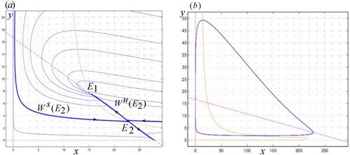
Theorem 3.5

For a suitable selection of parameter values, there exists a homoclinic curve determine by the stable and unstable manifold of the point $E_2(x_2,r(1-x_2/K\left)/b\right)$ $($Figure  1(a)$)$.

Proof.

Consider the point $(x,y)\in \overline{E_1{E}_2},$ then $\mathrm{d}x/\mathrm{d}t=0,\frac{\mathrm{d}y}{\mathrm{d}t}>0,$ we have that the direction of the vectors at points under the line $y=r(1-x/K)/b$ is pointing to the above.

Next, let $W_{+}^s\left(E_2\right)$ and $W_{+}^u\left(E_2\right)$ be the left stable manifold and the upper unstable manifold of the saddle point $E_2$, respectively. Then because we have by theorem 1 that ${\mathrm{\Sigma }}_0$ is an invariant region, the orbits cannot cross the horizontal line $y=y_{\max }-\left(c/b\right)x$ towards the above. The trajectories determined by the upper unstable manifold $W_{+}^u\left(E_2\right)$ cannot cross the trajectory determined by the left stable manifold $W_{+}^s\left(E_2\right)$. Moreover, the $\alpha -limit$ of the manifold $W_{+}^s\left(E_2\right)$ could be the origin or at infinity in the upper direction of the y−axis. On the other hand, the $\omega -limit$ of the upper unstable manifold $W_{+}^u\left(E_2\right)$ must be

1. the equilibrium $E_1,$ whenever this point is an stable node; or

2. the equilibrium $(K,0),$ whenever this point is an stable node,

then there exists a set of parameter values for which $W_{+}^u\left(E_2\right)$ intersects $W_{+}^s\left(E_2\right)$ and a homoclinic curve is generated. In this case, the point $E_2$ is the $\omega -limit$ of the upper unstable manifold $W_{+}^u\left(E_2\right)$.

3.2. Dynamic properties of the control system

We discuss existence,uniqueness and stability of the order-1 periodic orbit of system (3(3) $\left\{\begin{array}{l}\left.\begin{array}{c}\frac{\mathrm{d}x\left(t\right)}{\mathrm{d}t}=rx\left(t\right)\left(1-\frac{x\left(t\right)}{K}\right)-bx\left(t\right)y\left(t\right),\\ \frac{\mathrm{d}y\left(t\right)}{\mathrm{d}t}=cx\left(t\right)y\left(t\right)\frac{y\left(t\right)}{y\left(t\right)+m}-\mathrm{d}y\left(t\right),\end{array}\right\}x<x_T,\\ \left.\begin{array}{c}\mathrm{\Delta }x\left(t\right)=-p\left(x_T\right)x\left(t\right)\\ \mathrm{\Delta }y\left(t\right)=-q\left(x_T\right)y\left(t\right)+\tau \left(x_T\right)\end{array}\right\}x=x_T.\end{array}\right.$(3) ) based on the qualitative analysis of system (1(1) $\begin{array}{rl}& \frac{\mathrm{d}x\left(t\right)}{\mathrm{d}t}=rx\left(t\right)\left(1-\frac{x\left(t\right)}{K}\right)-bx\left(t\right)y\left(t\right),\\ & \frac{\mathrm{d}y\left(t\right)}{\mathrm{d}t}=cx\left(t\right)y\left(t\right)\frac{y\left(t\right)}{y\left(t\right)+m}-\mathrm{d}y\left(t\right).\end{array}$(1) ). Denote $p\left(x_T\right)\triangleq p_T$, $q\left(x_T\right)\triangleq q_T$, $\tau \left(x_T\right)\triangleq {\tau }_T.$ The strength of insecticide spraying to the pest is denoted as $p_T$. The larger $p_T$ is, the greater the strength is.

3.2.1. Existence of the order-1 periodic orbit

Denote Q as $Q\left(\right(1-p_T)x_T,{\tau }_T).$ The intersection points between the isocline $\dot{x}/x=0$ and the lines $x=(1-p_T)x_T$ and $x=x_T$ are denoted as $A\left(\right(1-p_T)x_T,y_A)$ and $B(x_T,y_B),$ where $y_A=r(1-(1-p_T\left)x_T/K\right)/b,y_B=r(1-x_T/K)/b=y_{x_T}.$ Denote $A^{-}(x_T,y_{A^{-}})$ and $Q^{-}(x_T,y_{Q^{-}})$ as the intersection points between $x=x_T$ and the trajectory starting from A and Q respectively. Obviously, we obtain $y_{Q^{-}}<y_{A^{-}}$.

We denote the pulse set as $M=\left\{\right(x,y)|x=x_T,y\ge 0\},$ and the phase set as $N\left\{\right(x,y)|x=(1-p_T)x_T,y\ge {\tau }_T\}.$

▪	The case for $H_1,H_2$

System (1(1) $\begin{array}{rl}& \frac{\mathrm{d}x\left(t\right)}{\mathrm{d}t}=rx\left(t\right)\left(1-\frac{x\left(t\right)}{K}\right)-bx\left(t\right)y\left(t\right),\\ & \frac{\mathrm{d}y\left(t\right)}{\mathrm{d}t}=cx\left(t\right)y\left(t\right)\frac{y\left(t\right)}{y\left(t\right)+m}-\mathrm{d}y\left(t\right).\end{array}$(1) ) has two positive equilibria: $E_1,E_2,$ and $E_1$ is stable, $E_2$ is a saddle point, but it has no limit cycle in ${\mathrm{\Sigma }}_0$ in the case of $H_1,H_2.$ The trajectory starting from the point A interests the impulsive set M at point $A^{-},$ and then jumps to the point $A^{+}.$ Define ${\overline{\tau }}_1\triangleq \frac{r}{b}\left(1-\frac{(1-p_T)x_T}{K}\right)-(1-q_T)y_{A^{-}}.$ According to the magnitude of $x_1,x_2$ and $X_T,$ the following three cases are discussed:

• Case I: $x_{ZX}\le x_T\le x_1$

Theorem 3.6

If $x_{ZX}\le x_T\le x_1,$ then system (3(3) $\left\{\begin{array}{l}\left.\begin{array}{c}\frac{\mathrm{d}x\left(t\right)}{\mathrm{d}t}=rx\left(t\right)\left(1-\frac{x\left(t\right)}{K}\right)-bx\left(t\right)y\left(t\right),\\ \frac{\mathrm{d}y\left(t\right)}{\mathrm{d}t}=cx\left(t\right)y\left(t\right)\frac{y\left(t\right)}{y\left(t\right)+m}-\mathrm{d}y\left(t\right),\end{array}\right\}x<x_T,\\ \left.\begin{array}{c}\mathrm{\Delta }x\left(t\right)=-p\left(x_T\right)x\left(t\right)\\ \mathrm{\Delta }y\left(t\right)=-q\left(x_T\right)y\left(t\right)+\tau \left(x_T\right)\end{array}\right\}x=x_T.\end{array}\right.$(3) ) has at least one order-1 periodic solution when ${\tau }_T\le {\overline{\tau }}_1,$ it has a unique order-1 periodic solution when ${\tau }_T>{\overline{\tau }}_1.$

Proof.

To prove the existence of order-1 periodic solution, we need find a point $L\in N$ such that $f_{\mathrm{sor}}\left(L\right)=0.$ According to the magnitudes between ${\overline{\tau }}_1$ and ${\tau }_T,$ two cases will be discussed.

(a) ${\tau }_T\le {\overline{\tau }}_1.$ Then the orbit $\widehat{A{A}^{-}{A}^{+}}$ is an order-1 periodic orbit when ${\tau }_T={\overline{\tau }}_1.$ The successor function of point A satisfies $f_{\mathrm{sor}}\left(A\right)=y_{A^{+}}-y_A<0$ when ${\tau }_T<{\overline{\tau }}_1.$ Choosing Q as the point in the phase set N with $y_Q={\tau }_T,$ thus $f_{\mathrm{sor}}\left(Q\right)=y_{Q^{+}}-y_Q>0.$ By the continuity of $f_{\mathrm{sor}},$ there exists at least a point $L\in \overline{AQ}\subset N$ such that $f_{\mathrm{sor}}\left(L\right)=0$, so system (3(3) $\left\{\begin{array}{l}\left.\begin{array}{c}\frac{\mathrm{d}x\left(t\right)}{\mathrm{d}t}=rx\left(t\right)\left(1-\frac{x\left(t\right)}{K}\right)-bx\left(t\right)y\left(t\right),\\ \frac{\mathrm{d}y\left(t\right)}{\mathrm{d}t}=cx\left(t\right)y\left(t\right)\frac{y\left(t\right)}{y\left(t\right)+m}-\mathrm{d}y\left(t\right),\end{array}\right\}x<x_T,\\ \left.\begin{array}{c}\mathrm{\Delta }x\left(t\right)=-p\left(x_T\right)x\left(t\right)\\ \mathrm{\Delta }y\left(t\right)=-q\left(x_T\right)y\left(t\right)+\tau \left(x_T\right)\end{array}\right\}x=x_T.\end{array}\right.$(3) ) has at least one order-1 periodic solution which passes through point L, as shown in Figure 2(a).

Figure 2. The existence of order-1 periodic solution of system (3(3) $\left\{\begin{array}{l}\left.\begin{array}{c}\frac{\mathrm{d}x\left(t\right)}{\mathrm{d}t}=rx\left(t\right)\left(1-\frac{x\left(t\right)}{K}\right)-bx\left(t\right)y\left(t\right),\\ \frac{\mathrm{d}y\left(t\right)}{\mathrm{d}t}=cx\left(t\right)y\left(t\right)\frac{y\left(t\right)}{y\left(t\right)+m}-\mathrm{d}y\left(t\right),\end{array}\right\}x<x_T,\\ \left.\begin{array}{c}\mathrm{\Delta }x\left(t\right)=-p\left(x_T\right)x\left(t\right)\\ \mathrm{\Delta }y\left(t\right)=-q\left(x_T\right)y\left(t\right)+\tau \left(x_T\right)\end{array}\right\}x=x_T.\end{array}\right.$(3) ) when $x_{ZX}\le x_T\le x_1,$ (a)${\tau }_T\le {\overline{\tau }}_1;$ (b)${\tau }_T>{\overline{\tau }}_1.$

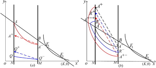
(b) ${\tau }_T>{\overline{\tau }}_1,$ then the successor function of point A satisfies $f_{\mathrm{sor}}\left(A\right)=y_{A^{+}}-y_A>0,$ and then $f_{\mathrm{sor}}\left(A^{+}\right)=(1-q_T)y_{A^{+-}}+{\tau }_T-y_{A^{+}}<(1-q_T)y_{A^{-}}+{\tau }_T-y_{A^{+}}=0.$ Let $R\left(\right(1-p_T)x_T,y_R)\in \overline{A{A}^{+}}$ such that $|y_R-y_{R^{+}}|<f_{\mathrm{sor}}\left(A\right),y_R-y_A<q_T{f}_{\mathrm{sor}}\left(A\right).$ So we have $f_{\mathrm{sor}}\left(R\right)=y_{R^{+}}-y_R>y_{A^{+}}-(1-q_T)f_{\mathrm{sor}}\left(A\right)-y_R=y_A+q_T{f}_{\mathrm{sor}}\left(A\right)-y_R>0.$ According to the continuity of $f_{\mathrm{sor}},$ there exists at least a point $L\in \overline{R{A}^{+}}\subset N$ such that $f_{\mathrm{sor}}\left(L\right)=0$, so the system (3(3) $\left\{\begin{array}{l}\left.\begin{array}{c}\frac{\mathrm{d}x\left(t\right)}{\mathrm{d}t}=rx\left(t\right)\left(1-\frac{x\left(t\right)}{K}\right)-bx\left(t\right)y\left(t\right),\\ \frac{\mathrm{d}y\left(t\right)}{\mathrm{d}t}=cx\left(t\right)y\left(t\right)\frac{y\left(t\right)}{y\left(t\right)+m}-\mathrm{d}y\left(t\right),\end{array}\right\}x<x_T,\\ \left.\begin{array}{c}\mathrm{\Delta }x\left(t\right)=-p\left(x_T\right)x\left(t\right)\\ \mathrm{\Delta }y\left(t\right)=-q\left(x_T\right)y\left(t\right)+\tau \left(x_T\right)\end{array}\right\}x=x_T.\end{array}\right.$(3) ) has an order-1 periodic solution which passes through point L, as shown in Figure 2(b).

In the following part, we discuss the uniqueness of the order-1 periodic solution to system (3(3) $\left\{\begin{array}{l}\left.\begin{array}{c}\frac{\mathrm{d}x\left(t\right)}{\mathrm{d}t}=rx\left(t\right)\left(1-\frac{x\left(t\right)}{K}\right)-bx\left(t\right)y\left(t\right),\\ \frac{\mathrm{d}y\left(t\right)}{\mathrm{d}t}=cx\left(t\right)y\left(t\right)\frac{y\left(t\right)}{y\left(t\right)+m}-\mathrm{d}y\left(t\right),\end{array}\right\}x<x_T,\\ \left.\begin{array}{c}\mathrm{\Delta }x\left(t\right)=-p\left(x_T\right)x\left(t\right)\\ \mathrm{\Delta }y\left(t\right)=-q\left(x_T\right)y\left(t\right)+\tau \left(x_T\right)\end{array}\right\}x=x_T.\end{array}\right.$(3) ). Select two points $L_1,L_2\in \overline{R{A}^{+}}\subset N$ arbitrarily, without loss of generality, we assume $x_{L_1}<x_{L_2}.$ Then there exist trajectories $l_{L_1}$ and $l_{L_2}$ passing $L_1$ and $L_2,$ and they cross the impulsive set M at $L_1^{-}$ and $L_2^{-},$ respectively. $L_1^{-}$ must be located on the right of $L_1^{+},$ we have $x_{L_1^{-}}>x_{L_2^{-}}.$ After impulsive effect, $L_1^{-}$ and $L_2^{-}$ jump to the phase set N at $L_1^{+}$ and $L_2^{+},$ respectively. Hence, $x_{L_1^{+}}>x_{L_2^{+}}.$ The successor functions of $L_1$ and $L_2$ are $f_{\mathrm{sor}}\left(L_1\right)$ and $f_{\mathrm{sor}}\left(L_2\right),$ then $f_{\mathrm{sor}}\left(L_1\right)-f_{\mathrm{sor}}\left(L_2\right)=x_{L_1^{+}}-x_{L_1}-(x_{L_2^{+}}-x_{L_2})=x_{L_1^{+}}-x_{L_2^{+}}+(x_{L_2}-x_{L_1})>0,$ which means the successor function $f_{\mathrm{sor}}$ is monotonically decreasing in the phase set. Thus, there exists a unique order-1 periodic solution.

• Case II: $x_1<x_T\le x_2$

In this case, there exists a trajectory $l_0$ of the system (3(3) $\left\{\begin{array}{l}\left.\begin{array}{c}\frac{\mathrm{d}x\left(t\right)}{\mathrm{d}t}=rx\left(t\right)\left(1-\frac{x\left(t\right)}{K}\right)-bx\left(t\right)y\left(t\right),\\ \frac{\mathrm{d}y\left(t\right)}{\mathrm{d}t}=cx\left(t\right)y\left(t\right)\frac{y\left(t\right)}{y\left(t\right)+m}-\mathrm{d}y\left(t\right),\end{array}\right\}x<x_T,\\ \left.\begin{array}{c}\mathrm{\Delta }x\left(t\right)=-p\left(x_T\right)x\left(t\right)\\ \mathrm{\Delta }y\left(t\right)=-q\left(x_T\right)y\left(t\right)+\tau \left(x_T\right)\end{array}\right\}x=x_T.\end{array}\right.$(3) ) which is tangency to the impulsive set M at point $B(x_T,y_B)$ and intersects the isocline $\dot{x}/x=0$ at point $C_0$ with $x_{C_0}<x_B=x_T.$ If there are intersection points between the trajectory $l_0$ and the phase set N, denoted by $C_1$ and $C_2$ with $y_{C_1}<y_{C_2}.$

Theorem 3.7

(1) If $x_1<x_T\le x_{2}and0<(1-p_T)x_T\le x_{C_0},$ then system (3(3) $\left\{\begin{array}{l}\left.\begin{array}{c}\frac{\mathrm{d}x\left(t\right)}{\mathrm{d}t}=rx\left(t\right)\left(1-\frac{x\left(t\right)}{K}\right)-bx\left(t\right)y\left(t\right),\\ \frac{\mathrm{d}y\left(t\right)}{\mathrm{d}t}=cx\left(t\right)y\left(t\right)\frac{y\left(t\right)}{y\left(t\right)+m}-\mathrm{d}y\left(t\right),\end{array}\right\}x<x_T,\\ \left.\begin{array}{c}\mathrm{\Delta }x\left(t\right)=-p\left(x_T\right)x\left(t\right)\\ \mathrm{\Delta }y\left(t\right)=-q\left(x_T\right)y\left(t\right)+\tau \left(x_T\right)\end{array}\right\}x=x_T.\end{array}\right.$(3) ) has an order-1 periodic solution. (2) If $x_1<x_T\le x_{2}and(1-p_T)x_T>x_{C_0},$ then system (3(3) $\left\{\begin{array}{l}\left.\begin{array}{c}\frac{\mathrm{d}x\left(t\right)}{\mathrm{d}t}=rx\left(t\right)\left(1-\frac{x\left(t\right)}{K}\right)-bx\left(t\right)y\left(t\right),\\ \frac{\mathrm{d}y\left(t\right)}{\mathrm{d}t}=cx\left(t\right)y\left(t\right)\frac{y\left(t\right)}{y\left(t\right)+m}-\mathrm{d}y\left(t\right),\end{array}\right\}x<x_T,\\ \left.\begin{array}{c}\mathrm{\Delta }x\left(t\right)=-p\left(x_T\right)x\left(t\right)\\ \mathrm{\Delta }y\left(t\right)=-q\left(x_T\right)y\left(t\right)+\tau \left(x_T\right)\end{array}\right\}x=x_T.\end{array}\right.$(3) ) has an order-1 periodic solution when ${\tau }_T\le {\overline{\tau }}_2\triangleq y_{C_1}-(1-q_T)y_B$ or ${\tau }_T\ge {\overline{\tau }}_3\triangleq y_{C_2}-(1-q_T)y_B.$

Proof.

(1) If $x_1<x_T\le x_2\mathrm{and}0<(1-p_T)x_T\le x_{C_0},$ then system (3(3) $\left\{\begin{array}{l}\left.\begin{array}{c}\frac{\mathrm{d}x\left(t\right)}{\mathrm{d}t}=rx\left(t\right)\left(1-\frac{x\left(t\right)}{K}\right)-bx\left(t\right)y\left(t\right),\\ \frac{\mathrm{d}y\left(t\right)}{\mathrm{d}t}=cx\left(t\right)y\left(t\right)\frac{y\left(t\right)}{y\left(t\right)+m}-\mathrm{d}y\left(t\right),\end{array}\right\}x<x_T,\\ \left.\begin{array}{c}\mathrm{\Delta }x\left(t\right)=-p\left(x_T\right)x\left(t\right)\\ \mathrm{\Delta }y\left(t\right)=-q\left(x_T\right)y\left(t\right)+\tau \left(x_T\right)\end{array}\right\}x=x_T.\end{array}\right.$(3) ) has at least one order-1 periodic solution when ${\tau }_T\le {\overline{\tau }}_1,$ it has a unique order-1 periodic solution when ${\tau }_T>{\overline{\tau }}_1.$ The proof is similar to that of Theorem 3.6 and omitted thereby, as illustrated in Figure 3(a,b).

Figure 3. The existence of order-1 periodic solution of system (3(3) $\left\{\begin{array}{l}\left.\begin{array}{c}\frac{\mathrm{d}x\left(t\right)}{\mathrm{d}t}=rx\left(t\right)\left(1-\frac{x\left(t\right)}{K}\right)-bx\left(t\right)y\left(t\right),\\ \frac{\mathrm{d}y\left(t\right)}{\mathrm{d}t}=cx\left(t\right)y\left(t\right)\frac{y\left(t\right)}{y\left(t\right)+m}-\mathrm{d}y\left(t\right),\end{array}\right\}x<x_T,\\ \left.\begin{array}{c}\mathrm{\Delta }x\left(t\right)=-p\left(x_T\right)x\left(t\right)\\ \mathrm{\Delta }y\left(t\right)=-q\left(x_T\right)y\left(t\right)+\tau \left(x_T\right)\end{array}\right\}x=x_T.\end{array}\right.$(3) ) when $x_1<x_T\le x_2$, (a) $0<(1-p_T)x_T\le x_{C_0}\mathrm{and}{\tau }_T\le {\overline{\tau }}_1$; (b) $0<(1-p_T)x_T\le x_{C_0}\mathrm{and}{\tau }_T>{\overline{\tau }}_1$; (c) $(1-p_T)x_T>x_{C_0}$.

(2) If $x_1<x_T\le x_2$ and $(1-p_T)x_T>x_{C_0}$, as shown in Figure 3(c). Then there is $f_{\mathrm{sor}}\left(C_1\right)\le 0$ when ${\tau }_T\le {\overline{\tau }}_2,$ note that $f_{\mathrm{sor}}\left(Q\right)>0,$ thus there exists $L\in \overline{Q{C}_1}$ such that $f_{\mathrm{sor}}\left(L\right)=0.$ When ${\overline{\tau }}_2<{\tau }_T<{\overline{\tau }}_3,$ the trajectory will tend to the equilibrium point $E_1$ by the stability of point $E_1.$ So the system (3(3) $\left\{\begin{array}{l}\left.\begin{array}{c}\frac{\mathrm{d}x\left(t\right)}{\mathrm{d}t}=rx\left(t\right)\left(1-\frac{x\left(t\right)}{K}\right)-bx\left(t\right)y\left(t\right),\\ \frac{\mathrm{d}y\left(t\right)}{\mathrm{d}t}=cx\left(t\right)y\left(t\right)\frac{y\left(t\right)}{y\left(t\right)+m}-\mathrm{d}y\left(t\right),\end{array}\right\}x<x_T,\\ \left.\begin{array}{c}\mathrm{\Delta }x\left(t\right)=-p\left(x_T\right)x\left(t\right)\\ \mathrm{\Delta }y\left(t\right)=-q\left(x_T\right)y\left(t\right)+\tau \left(x_T\right)\end{array}\right\}x=x_T.\end{array}\right.$(3) ) has no order-1 periodic solution. When ${\tau }_T\ge {\overline{\tau }}_3,$ there is $f_{\mathrm{sor}}\left(C_2\right)\ge 0$ and $f_{\mathrm{sor}}\left(C_2^{+}\right)<0,$ thus there exists $L\in \overline{C_2{C}_2^{+}}$ such that $f_{\mathrm{sor}}\left(L\right)=0,$ the proof of the uniqueness is similar to that of Theorem 3.6.

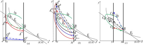
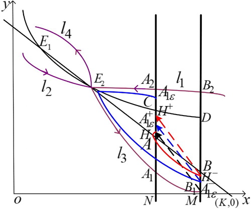
• Case III: $x_2<x_T\le min\{x_{ZD},K\}$

Assume that $l_1,l_2,l_3,l_4$ are dividing lines of the saddle point $E_2(x_2,y_2)$, where $l_1,l_2$ are the stable flows of $E_2(x_2,y_2),$ $l_3,l_4$ are the unstable flows of $E_2(x_2,y_2).$ Let $C_0(x_{C_0},y_{C_0})$ denote the intersection point between the isocline $\dot{x}/x=0$ and the stable flow $l_2$ with $x_{C_0}<x_{E_2},$ as illustrated in Figure 4. According to the magnitude of $(1-p_T)x_T,x_2$ and $x_{C_0},$ there exist three cases:

Figure 4. The existence of order-1 periodic solution of system (3(3) $\left\{\begin{array}{l}\left.\begin{array}{c}\frac{\mathrm{d}x\left(t\right)}{\mathrm{d}t}=rx\left(t\right)\left(1-\frac{x\left(t\right)}{K}\right)-bx\left(t\right)y\left(t\right),\\ \frac{\mathrm{d}y\left(t\right)}{\mathrm{d}t}=cx\left(t\right)y\left(t\right)\frac{y\left(t\right)}{y\left(t\right)+m}-\mathrm{d}y\left(t\right),\end{array}\right\}x<x_T,\\ \left.\begin{array}{c}\mathrm{\Delta }x\left(t\right)=-p\left(x_T\right)x\left(t\right)\\ \mathrm{\Delta }y\left(t\right)=-q\left(x_T\right)y\left(t\right)+\tau \left(x_T\right)\end{array}\right\}x=x_T.\end{array}\right.$(3) ) when $x_2<x_T\le \min \{x_{ZD},K\}$, (a) $0<(1-p_T)x_T\le x_{C_0}\mathrm{and}{\tau }_T\le {\overline{\tau }}_1$; (b) $0<(1-p_T)x_T\le x_{C_0}\mathrm{and}{\tau }_T>{\overline{\tau }}_1$; (c) $(1-p_T)x_T>x_{C_0}$.

(a) $(1-p_T)x_T\le x_{C_0},$ the case is similar to that of Theorem 3.6, as illustrated in Figure 4(a,b);

(b) $x_{C_0}<(1-p_T)x_T<x_2,$ denote $C_1$ and $C_2$ as the intersection points between $x=(1-p_T)x_T$ and stable flow $l_2$ with $y_{C_1}<y_{C_2}.$ And the unstable flow $l_3$ intersects $x=x_T$ at point $C_1^{-}.$ There is $f_{\mathrm{sor}}\left(C_1\right)<0$ when ${\tau }_T<{\overline{\tau }}_4\triangleq y_{C_1}-(1-q_T)y_{C_1^{-}},$ note that $f_{\mathrm{sor}}\left(Q\right)>0,$ thus there exists $L\in \overline{Q{C}_1}$ such that $f_{\mathrm{sor}}\left(L\right)=0.$ When ${\overline{\tau }}_4<{\tau }_T<{\overline{\tau }}_5\triangleq y_{C_2}-(1-q_T)y_{C_1^{-}},$ the trajectory will tend to the equilibrium point $E_1$ by the stability of point $E_1.$ So system (3(3) $\left\{\begin{array}{l}\left.\begin{array}{c}\frac{\mathrm{d}x\left(t\right)}{\mathrm{d}t}=rx\left(t\right)\left(1-\frac{x\left(t\right)}{K}\right)-bx\left(t\right)y\left(t\right),\\ \frac{\mathrm{d}y\left(t\right)}{\mathrm{d}t}=cx\left(t\right)y\left(t\right)\frac{y\left(t\right)}{y\left(t\right)+m}-\mathrm{d}y\left(t\right),\end{array}\right\}x<x_T,\\ \left.\begin{array}{c}\mathrm{\Delta }x\left(t\right)=-p\left(x_T\right)x\left(t\right)\\ \mathrm{\Delta }y\left(t\right)=-q\left(x_T\right)y\left(t\right)+\tau \left(x_T\right)\end{array}\right\}x=x_T.\end{array}\right.$(3) ) has no order-1 periodic solution. When ${\tau }_T>{\overline{\tau }}_5,$ there is $f_{\mathrm{sor}}\left(C_2\right)>0$ and $f_{\mathrm{sor}}\left(C_2^{+}\right)<0,$ thus there exists $L\in \overline{C_2{C}_2^{+}}$ such that $f_{\mathrm{sor}}\left(L\right)=0,$ as shown in Figure 4(c).

(c) $x_2\le (1-p_T)x_T<x_T\le x_{ZD},$ assume that the unstable flows $l_3$ and the stable flows $l_1$ intersect $x=(1-p_T)x_T,x=x_T$ at points $A_1,B_1$ and $A_2,B_2,$ respectively. Suppose that the isocline $\dot{x}/x=0$ and $\dot{y}/y=0$ intersect the line $x=(1-p_T)x_T,x=x_T$ at points A,B and $C,D,$ respectively.

Then there must exist ${\tau }^1,{\tau }^2$ such that $(1-q_T)y_{B_1}+{\tau }^1=y_A,(1-q_T)y_{B_1}+{\tau }^2=y_{A_2}.$ It can be deduced that the point $B_1$ is mapped into A if ${\tau }_T={\tau }^1$ and it is mapped into $A_2$ if ${\tau }_T={\tau }^2.$ Therefore, applying the definition of the homoclinic cycle, we obtain that the trajectories $\widetilde{A_2{E}_2},\widetilde{E_2{B}_1}$ together with the impulsive line $\overline{B_1{A}_2}$ constitute a homoclinic cycle for the system (3(3) $\left\{\begin{array}{l}\left.\begin{array}{c}\frac{\mathrm{d}x\left(t\right)}{\mathrm{d}t}=rx\left(t\right)\left(1-\frac{x\left(t\right)}{K}\right)-bx\left(t\right)y\left(t\right),\\ \frac{\mathrm{d}y\left(t\right)}{\mathrm{d}t}=cx\left(t\right)y\left(t\right)\frac{y\left(t\right)}{y\left(t\right)+m}-\mathrm{d}y\left(t\right),\end{array}\right\}x<x_T,\\ \left.\begin{array}{c}\mathrm{\Delta }x\left(t\right)=-p\left(x_T\right)x\left(t\right)\\ \mathrm{\Delta }y\left(t\right)=-q\left(x_T\right)y\left(t\right)+\tau \left(x_T\right)\end{array}\right\}x=x_T.\end{array}\right.$(3) ) when ${\tau }_T={\tau }^2.$

Theorem 3.8

When $x_2\le (1-p_T)x_T<x_T\le x_{ZD},$ there exist ${\tau }^1,{\tau }^2$ such that for any ${\tau }_T\in ({\tau }^1,{\tau }^2),$ the order-1 homoclinic cycle disappears and system (3(3) $\left\{\begin{array}{l}\left.\begin{array}{c}\frac{\mathrm{d}x\left(t\right)}{\mathrm{d}t}=rx\left(t\right)\left(1-\frac{x\left(t\right)}{K}\right)-bx\left(t\right)y\left(t\right),\\ \frac{\mathrm{d}y\left(t\right)}{\mathrm{d}t}=cx\left(t\right)y\left(t\right)\frac{y\left(t\right)}{y\left(t\right)+m}-\mathrm{d}y\left(t\right),\end{array}\right\}x<x_T,\\ \left.\begin{array}{c}\mathrm{\Delta }x\left(t\right)=-p\left(x_T\right)x\left(t\right)\\ \mathrm{\Delta }y\left(t\right)=-q\left(x_T\right)y\left(t\right)+\tau \left(x_T\right)\end{array}\right\}x=x_T.\end{array}\right.$(3) ) bifurcates a unique order-1 positive periodic solution.

Proof.

Denote H as the image point of $B_1,$ for any ${\tau }_T\in ({\tau }^1,{\tau }^2),$ there is $y_H=(1-q_T)y_{B_1}+{\tau }_T\in \left(\right(1-q_T)y_{B_1}+{\tau }^1,(1-q_T)y_{B_1}+{\tau }^2)=(y_A,y_{A_2}),$ and H is between A and $A_2$. Assume that the trajectory starting from the point H firstly intersects the line $x=x_T$ at point $H^{-}$ and then jumps into $H^{+}$ because of the impulsive effect. On account that any two trajectories of autonomous systems cannot intersect, so $y_{H^{-}}>y_{B_1}$. Thus, $y_{H^{+}}>y_H$ and the successor function satisfies $f_{\mathrm{sor}}\left(H\right)=y_{H^{+}}-y_H>0.$ In another aspect, we take a point $A_{1ϵ}\left(\right(1-p_T)x_T,y_{A_{1ϵ}})$ where $y_{A_{1ϵ}}=y_{A_2}-ϵ$ and $ϵ>0$ is sufficiently small. Assume that the trajectory with the initial point $A_{1ϵ}$ firstly intersects $x=x_T$ at a point $A_{1ϵ}^{-}$ and then jumps into $A_{1ϵ}^{+}$ when the impulse occurs. $A_{1ϵ}^{-}$ is next to point $B_1$ which can be inferred from the continuous dependence of the solution concerning the initial value. Then $f_{\mathrm{sor}}\left(A_{1ϵ}\right)=y_{A_{1ϵ}^{+}}-y_{A_{1ϵ}}<0.$ So there must exist a point $L\in \overline{A_{1ϵ}H}$ such that $f_{\mathrm{sor}}\left(L\right)=0.$ Therefore, system (3(3) $\left\{\begin{array}{l}\left.\begin{array}{c}\frac{\mathrm{d}x\left(t\right)}{\mathrm{d}t}=rx\left(t\right)\left(1-\frac{x\left(t\right)}{K}\right)-bx\left(t\right)y\left(t\right),\\ \frac{\mathrm{d}y\left(t\right)}{\mathrm{d}t}=cx\left(t\right)y\left(t\right)\frac{y\left(t\right)}{y\left(t\right)+m}-\mathrm{d}y\left(t\right),\end{array}\right\}x<x_T,\\ \left.\begin{array}{c}\mathrm{\Delta }x\left(t\right)=-p\left(x_T\right)x\left(t\right)\\ \mathrm{\Delta }y\left(t\right)=-q\left(x_T\right)y\left(t\right)+\tau \left(x_T\right)\end{array}\right\}x=x_T.\end{array}\right.$(3) ) has at least a positive order-1 periodic solution and the geometrical interpretation is as shown in Figure 5.

Figure 5. The existence of order-1 periodic solution of system (3(3) $\left\{\begin{array}{l}\left.\begin{array}{c}\frac{\mathrm{d}x\left(t\right)}{\mathrm{d}t}=rx\left(t\right)\left(1-\frac{x\left(t\right)}{K}\right)-bx\left(t\right)y\left(t\right),\\ \frac{\mathrm{d}y\left(t\right)}{\mathrm{d}t}=cx\left(t\right)y\left(t\right)\frac{y\left(t\right)}{y\left(t\right)+m}-\mathrm{d}y\left(t\right),\end{array}\right\}x<x_T,\\ \left.\begin{array}{c}\mathrm{\Delta }x\left(t\right)=-p\left(x_T\right)x\left(t\right)\\ \mathrm{\Delta }y\left(t\right)=-q\left(x_T\right)y\left(t\right)+\tau \left(x_T\right)\end{array}\right\}x=x_T.\end{array}\right.$(3) ) when $x_2\le (1-p_{x_T})x_T<x_T\le x_{ZD},{\tau }_T\in ({\tau }^1,{\tau }^2)$.

Next, the uniqueness of the positive order-1 periodic solution will be proved. Take any two points $L_1,L_2\in \overline{A_{1ϵ}H}$ with $y_{L_1}<y_{L_2}.$ Suppose that the respective trajectories with these two starting points are $L_1\to L_1^{-}\to L_1^{+},L_2\to L_2^{-}\to L_2^{+},$ where $L_1^{+},L_2^{+}$ are the first successor points for $L_1$ and $L_2,$ respectively. We obtain $y_{L_2^{-}}<y_{L_1^{-}}$ from $y_{L_1}<y_{L_2}.$ Then $y_{L_2^{+}}=(1-q_T)y_{L_2^{-}}+{\tau }_T<(1-q_T)y_{L_1^{-}}+{\tau }_T=y_{L_1^{+}}.$ Thus $f_{\mathrm{sor}}\left(L_1\right)-f_{\mathrm{sor}}\left(L_2\right)=y_{L_1^{+}}-y_{L_1}-(y_{L_2^{+}}-y_{L_2})=(y_{L_2}-y_{L_1})+(y_{L_1^{+}}-y_{L_2^{+}})>0$ which implies that $f_{\mathrm{sor}}$ is a monotone decreasing function. Notably, $L_1$ and $L_2$ are arbitrary in the line $\overline{A_{1ϵ}H}.$ Therefore, there exists a unique point L such that $f_{\mathrm{sor}}\left(L\right)=0,$ and it follows from the property of the $Poincar\acute{e}$ map that the bifurcated positive periodic solution is unique.

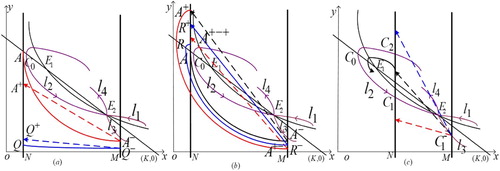
According to Theorem 3.5, when the homoclinic curve disappears, it has two situations by the position relationship between the stable flow $l_2$ and the unstable flow $l_4.$

(i) If the unstable flow $l_4$ is outside of the stable flow $l_2,$ three kinds of situations (see Figure 6(a)): ${\tau }_T\le {\overline{\tau }}_6=y_{A_2}-(1-q_T)y_{A^{-}},$ there exists an order-1 periodic solution from the proof of Theorem 3.6(a); ${\overline{\tau }}_1<{\tau }_T<{\overline{\tau }}_6=y_{A_2}-(1-q_T)y_{A^{-}},$ there exists a unique order-1 periodic solution from the proof of Theorem 3.8; ${\tau }_T>{\overline{\tau }}_6,$ there exists a unique order-1 periodic solution from the proof of Theorem 3.6(b) and omitted thereby.

Figure 6. The existence of order-1 periodic solution of system (3(3) $\left\{\begin{array}{l}\left.\begin{array}{c}\frac{\mathrm{d}x\left(t\right)}{\mathrm{d}t}=rx\left(t\right)\left(1-\frac{x\left(t\right)}{K}\right)-bx\left(t\right)y\left(t\right),\\ \frac{\mathrm{d}y\left(t\right)}{\mathrm{d}t}=cx\left(t\right)y\left(t\right)\frac{y\left(t\right)}{y\left(t\right)+m}-\mathrm{d}y\left(t\right),\end{array}\right\}x<x_T,\\ \left.\begin{array}{c}\mathrm{\Delta }x\left(t\right)=-p\left(x_T\right)x\left(t\right)\\ \mathrm{\Delta }y\left(t\right)=-q\left(x_T\right)y\left(t\right)+\tau \left(x_T\right)\end{array}\right\}x=x_T.\end{array}\right.$(3) ) when $x_2\le (1-p_T)x_T<x_T\le \min \{x_{ZD},K\},$ (a)the unstable flow $l_4$ is outside of the stable flow $l_2;$ (b)the stable flow $l_2$ is outside of the unstable flow $l_4.$

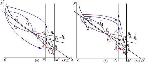
(ii) If the stable flow $l_2$ is outside of the unstable flow $l_4,$ the stable flow $l_2$ intersects the phase set N at point F as $t\to -\mathrm{\infty }.$ There are four kinds of situations (see Figure 6(b)):${\tau }_T\le {\overline{\tau }}_1,$ it is similar to that of Theorem 3.6(a); ${\overline{\tau }}_1<{\tau }_T\le {\overline{\tau }}_6=y_{A_2}-(1-q_T)y_{A^{-}},$ it is similar to that of Theorem 3.8; ${\overline{\tau }}_6<{\tau }_T\le {\overline{\tau }}_7=y_F-(1-q_T)y_{A^{-}},$ then by the stability of point $E_1,$ we know the trajectory will approach point $E_1;$ ${\tau }_T>{\overline{\tau }}_7,$ there exists a unique order-1 periodic solution.

▪	The case for $H_3$

System (1(1) $\begin{array}{rl}& \frac{\mathrm{d}x\left(t\right)}{\mathrm{d}t}=rx\left(t\right)\left(1-\frac{x\left(t\right)}{K}\right)-bx\left(t\right)y\left(t\right),\\ & \frac{\mathrm{d}y\left(t\right)}{\mathrm{d}t}=cx\left(t\right)y\left(t\right)\frac{y\left(t\right)}{y\left(t\right)+m}-\mathrm{d}y\left(t\right).\end{array}$(1) ) has two positive equilibria: $E_1,E_2,$ $E_1$ is unstable, $E_2$ is a saddle point, and it has a stable limit cycle around point $E_1$ in ${\mathrm{\Sigma }}_0$ in the case of $H_3.$ Denote the limit cycle by ${\mathrm{\Gamma }}_0.$ The limit cycle intersects the isoclinic line $\dot{x}/x=0$ at points $S_1(h_1,y_{S_1}),S_2(h_2,y_{S_2}),$ and $h_1<h_2.$

When $x_{ZX}<x_T<h_1<x_{ZD}or{x}_{ZX}\le (1-p_T)x_T<h_1<x_T\le h_2<x_{ZD},$ system (3(3) $\left\{\begin{array}{l}\left.\begin{array}{c}\frac{\mathrm{d}x\left(t\right)}{\mathrm{d}t}=rx\left(t\right)\left(1-\frac{x\left(t\right)}{K}\right)-bx\left(t\right)y\left(t\right),\\ \frac{\mathrm{d}y\left(t\right)}{\mathrm{d}t}=cx\left(t\right)y\left(t\right)\frac{y\left(t\right)}{y\left(t\right)+m}-\mathrm{d}y\left(t\right),\end{array}\right\}x<x_T,\\ \left.\begin{array}{c}\mathrm{\Delta }x\left(t\right)=-p\left(x_T\right)x\left(t\right)\\ \mathrm{\Delta }y\left(t\right)=-q\left(x_T\right)y\left(t\right)+\tau \left(x_T\right)\end{array}\right\}x=x_T.\end{array}\right.$(3) ) has an order-1 periodic solution from the proof of Theorem 3.6.

When $x_{ZX}\le (1-p_T)x_T<x_T<x_2<x_{ZD}$ system (3(3) $\left\{\begin{array}{l}\left.\begin{array}{c}\frac{\mathrm{d}x\left(t\right)}{\mathrm{d}t}=rx\left(t\right)\left(1-\frac{x\left(t\right)}{K}\right)-bx\left(t\right)y\left(t\right),\\ \frac{\mathrm{d}y\left(t\right)}{\mathrm{d}t}=cx\left(t\right)y\left(t\right)\frac{y\left(t\right)}{y\left(t\right)+m}-\mathrm{d}y\left(t\right),\end{array}\right\}x<x_T,\\ \left.\begin{array}{c}\mathrm{\Delta }x\left(t\right)=-p\left(x_T\right)x\left(t\right)\\ \mathrm{\Delta }y\left(t\right)=-q\left(x_T\right)y\left(t\right)+\tau \left(x_T\right)\end{array}\right\}x=x_T.\end{array}\right.$(3) ) has an order-1 periodic solution or the trajectories of system (3(3) $\left\{\begin{array}{l}\left.\begin{array}{c}\frac{\mathrm{d}x\left(t\right)}{\mathrm{d}t}=rx\left(t\right)\left(1-\frac{x\left(t\right)}{K}\right)-bx\left(t\right)y\left(t\right),\\ \frac{\mathrm{d}y\left(t\right)}{\mathrm{d}t}=cx\left(t\right)y\left(t\right)\frac{y\left(t\right)}{y\left(t\right)+m}-\mathrm{d}y\left(t\right),\end{array}\right\}x<x_T,\\ \left.\begin{array}{c}\mathrm{\Delta }x\left(t\right)=-p\left(x_T\right)x\left(t\right)\\ \mathrm{\Delta }y\left(t\right)=-q\left(x_T\right)y\left(t\right)+\tau \left(x_T\right)\end{array}\right\}x=x_T.\end{array}\right.$(3) ) tend to the limit cycle after finite times impulsive effects at most for $t\to +\mathrm{\infty }$ by Theorem 3.7.

When $x_{ZX}\le (1-p_T)x_T<x_2<x_T<x_{ZD}<K,$ the case is similar to that of case III (1) and (2).

When $min\{x_2,x_{ZX}\}<(1-p_T)x_T<x_T<x_{ZD}<K,$ the case is similar to that of case III (3).

Theorem 3.9

If $h_1<(1-p_T)x_T<x_T<h_2,$ then system (3(3) $\left\{\begin{array}{l}\left.\begin{array}{c}\frac{\mathrm{d}x\left(t\right)}{\mathrm{d}t}=rx\left(t\right)\left(1-\frac{x\left(t\right)}{K}\right)-bx\left(t\right)y\left(t\right),\\ \frac{\mathrm{d}y\left(t\right)}{\mathrm{d}t}=cx\left(t\right)y\left(t\right)\frac{y\left(t\right)}{y\left(t\right)+m}-\mathrm{d}y\left(t\right),\end{array}\right\}x<x_T,\\ \left.\begin{array}{c}\mathrm{\Delta }x\left(t\right)=-p\left(x_T\right)x\left(t\right)\\ \mathrm{\Delta }y\left(t\right)=-q\left(x_T\right)y\left(t\right)+\tau \left(x_T\right)\end{array}\right\}x=x_T.\end{array}\right.$(3) ) has at last four kinds of order-1 periodic solutions (the case for ${\tau }_T>{\overline{\tau }}_1$).

Proof.

When $x<x_1,$ the horizontal ordinate of the orbit passing through the isocline $\dot{x}/x=0$ increase with the increase of time, i.e. $\mathrm{d}x/\mathrm{d}t>0.$ Therefore, when $h_1<(1-p_T)x_T<x_T<h_2,$ there must exist a point $L_1\in M$ such that system (3(3) $\left\{\begin{array}{l}\left.\begin{array}{c}\frac{\mathrm{d}x\left(t\right)}{\mathrm{d}t}=rx\left(t\right)\left(1-\frac{x\left(t\right)}{K}\right)-bx\left(t\right)y\left(t\right),\\ \frac{\mathrm{d}y\left(t\right)}{\mathrm{d}t}=cx\left(t\right)y\left(t\right)\frac{y\left(t\right)}{y\left(t\right)+m}-\mathrm{d}y\left(t\right),\end{array}\right\}x<x_T,\\ \left.\begin{array}{c}\mathrm{\Delta }x\left(t\right)=-p\left(x_T\right)x\left(t\right)\\ \mathrm{\Delta }y\left(t\right)=-q\left(x_T\right)y\left(t\right)+\tau \left(x_T\right)\end{array}\right\}x=x_T.\end{array}\right.$(3) ) has an order-1 periodic solution which consists of $L_1,$ the phase point $L\in N$ of $L_1$ and the orbit between them (Figure 7(a,b and d)).

Figure 7. Four kinds of order-1 periodic solutions of system (3(3) $\left\{\begin{array}{l}\left.\begin{array}{c}\frac{\mathrm{d}x\left(t\right)}{\mathrm{d}t}=rx\left(t\right)\left(1-\frac{x\left(t\right)}{K}\right)-bx\left(t\right)y\left(t\right),\\ \frac{\mathrm{d}y\left(t\right)}{\mathrm{d}t}=cx\left(t\right)y\left(t\right)\frac{y\left(t\right)}{y\left(t\right)+m}-\mathrm{d}y\left(t\right),\end{array}\right\}x<x_T,\\ \left.\begin{array}{c}\mathrm{\Delta }x\left(t\right)=-p\left(x_T\right)x\left(t\right)\\ \mathrm{\Delta }y\left(t\right)=-q\left(x_T\right)y\left(t\right)+\tau \left(x_T\right)\end{array}\right\}x=x_T.\end{array}\right.$(3) ) when $h_1<(1-p_T)x_T<x_T<h_2.$

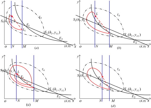
Since the limit cycle is table, then the orbits starting from the point in the limit cycle tend to the limit cycle. For the point $L_1(x_T,y_{L_1})$ close to the isocline $\dot{y}=0$ sufficiently, the trajectory passing through the point $L_1(x_T,y_{L_1})$ can intersect the line $y=\left(y_{L_1}{q}_T-{\tau }_T\right)/p_T{x}_{T}x+(1-(q_T/p_T\left)\right)y_{L_1}+\left({\tau }_T/p_T\right)$ of the impulsive function $\mathrm{\Delta }y=-q_{T}y+{\tau }_T$ at two points for $t\to -\mathrm{\infty },$ then system (3(3) $\left\{\begin{array}{l}\left.\begin{array}{c}\frac{\mathrm{d}x\left(t\right)}{\mathrm{d}t}=rx\left(t\right)\left(1-\frac{x\left(t\right)}{K}\right)-bx\left(t\right)y\left(t\right),\\ \frac{\mathrm{d}y\left(t\right)}{\mathrm{d}t}=cx\left(t\right)y\left(t\right)\frac{y\left(t\right)}{y\left(t\right)+m}-\mathrm{d}y\left(t\right),\end{array}\right\}x<x_T,\\ \left.\begin{array}{c}\mathrm{\Delta }x\left(t\right)=-p\left(x_T\right)x\left(t\right)\\ \mathrm{\Delta }y\left(t\right)=-q\left(x_T\right)y\left(t\right)+\tau \left(x_T\right)\end{array}\right\}x=x_T.\end{array}\right.$(3) ) has an order-1 periodic solution, see Figure 7(c). Particularly, the trajectory between L and $L_1$ can revolve round the equilibrium $E_1$ several cycles, which resembles Figure 7(c). This completes the proof.

3.2.2. Stability analysis of the order-1 periodic orbit

Denote ${\gamma }_L=\widehat{L{L}^{-}L}$ as the order-1 periodic orbit of system (3(3) $\left\{\begin{array}{l}\left.\begin{array}{c}\frac{\mathrm{d}x\left(t\right)}{\mathrm{d}t}=rx\left(t\right)\left(1-\frac{x\left(t\right)}{K}\right)-bx\left(t\right)y\left(t\right),\\ \frac{\mathrm{d}y\left(t\right)}{\mathrm{d}t}=cx\left(t\right)y\left(t\right)\frac{y\left(t\right)}{y\left(t\right)+m}-\mathrm{d}y\left(t\right),\end{array}\right\}x<x_T,\\ \left.\begin{array}{c}\mathrm{\Delta }x\left(t\right)=-p\left(x_T\right)x\left(t\right)\\ \mathrm{\Delta }y\left(t\right)=-q\left(x_T\right)y\left(t\right)+\tau \left(x_T\right)\end{array}\right\}x=x_T.\end{array}\right.$(3) ). Analysing the stability of the possible periodic orbit, the results are as follows.

Theorem 3.10

The order-1 periodic orbit ${\gamma }_L$ of system (3(3) $\left\{\begin{array}{l}\left.\begin{array}{c}\frac{\mathrm{d}x\left(t\right)}{\mathrm{d}t}=rx\left(t\right)\left(1-\frac{x\left(t\right)}{K}\right)-bx\left(t\right)y\left(t\right),\\ \frac{\mathrm{d}y\left(t\right)}{\mathrm{d}t}=cx\left(t\right)y\left(t\right)\frac{y\left(t\right)}{y\left(t\right)+m}-\mathrm{d}y\left(t\right),\end{array}\right\}x<x_T,\\ \left.\begin{array}{c}\mathrm{\Delta }x\left(t\right)=-p\left(x_T\right)x\left(t\right)\\ \mathrm{\Delta }y\left(t\right)=-q\left(x_T\right)y\left(t\right)+\tau \left(x_T\right)\end{array}\right\}x=x_T.\end{array}\right.$(3) ) is orbitally asymptotically stable if $x_2\le (1-p_T)x_T<x_T\le x_{ZD}and{\tau }_T\in ({\tau }^1,{\tau }^2).$

Proof.

Denote $H^{+}$ as $H_1,$ we need prove the sequence $\left\{y_{H_{2k}}\right\}$ is monotonically increasing and $\left\{y_{H_{2k-1}}\right\}$ is monotonically decreasing, where $H_{2k},H_{2k-1}(k=1,2,3,\dots )$ are successor points of H (Figure 8). On account of $y_L<y_{H_1}<y_{A_{1ϵ}},$ we obtain $y_H<y_{H_2}<y_L.$ Repeating the process, we have $y_L<y_{H_3}<y_{H_1}<y_{A_{1ϵ}},y_H<y_{H_2}<y_{H_4}<y_L.$ By induction, we get that $\left\{y_{H_{2k}}\right\}$ is monotonically increasing and $\left\{y_{H_{2k-1}}\right\}$ is monotonically decreasing. For any point $I\in \overline{H{A}_{1ϵ}},$ assume that $I\in \overline{HL},$ i.e. $y_H<y_I<y_L.$ Clearly, there must exist a positive integer i such that $y_{H_{2i}}<y_I<y_{H_{2(i+1)}}$. Assume that the iterates of I are given by $\{I_1,I_2,I_3,I_4,\dots \}.$ Thus, there are the following inequalities: $\begin{array}{rl}& y_L<y_{H_{2(i+1)+1}}<y_{I_1}<y_{H_{2i+1}}<y_{A_{1ϵ}},\\ & y_H<y_{H_{2(i+1)}}<y_{I_2}<y_{H_{2(i+2)}}<y_L,\\ & y_L<y_{H_{2(i+2)+1}}<y_{I_3}<y_{H_{2(i+1)+1}}<y_{A_{1ϵ}},\\ & y_H<y_{H_{2(i+1)}}<y_{H_{2(i+2)}}<y_{I_4}<y_{H_{2(i+3)}}<y_L.\end{array}$

Figure 8. The stability of the order-1 periodic solution of system (3(3) $\left\{\begin{array}{l}\left.\begin{array}{c}\frac{\mathrm{d}x\left(t\right)}{\mathrm{d}t}=rx\left(t\right)\left(1-\frac{x\left(t\right)}{K}\right)-bx\left(t\right)y\left(t\right),\\ \frac{\mathrm{d}y\left(t\right)}{\mathrm{d}t}=cx\left(t\right)y\left(t\right)\frac{y\left(t\right)}{y\left(t\right)+m}-\mathrm{d}y\left(t\right),\end{array}\right\}x<x_T,\\ \left.\begin{array}{c}\mathrm{\Delta }x\left(t\right)=-p\left(x_T\right)x\left(t\right)\\ \mathrm{\Delta }y\left(t\right)=-q\left(x_T\right)y\left(t\right)+\tau \left(x_T\right)\end{array}\right\}x=x_T.\end{array}\right.$(3) ) when ${\tau }_T\in ({\tau }^1,{\tau }^2).$

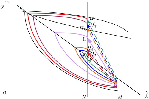
By the use of resembling arguments to those in the statement of $\left\{y_{H_{2k}}\right\}$ and $\left\{y_{H_{2k-1}}\right\},$ we can obtain inductively that $\left\{y_{I_{2k}}\right\}$ is monotonically increasing and $\left\{y_{I_{2k-1}}\right\}$ is monotonically decreasing. In addition, $\underset{k\to \mathrm{\infty }}{lim}{y}_{I_{2k-1}}=y_L,\underset{k\to \mathrm{\infty }}{lim}{y}_{I_{2k}}=y_L.$ Thus, the trajectory starting from point I will eventually attract to L. The order-1 periodic orbit ${\gamma }_L$ of system (3(3) $\left\{\begin{array}{l}\left.\begin{array}{c}\frac{\mathrm{d}x\left(t\right)}{\mathrm{d}t}=rx\left(t\right)\left(1-\frac{x\left(t\right)}{K}\right)-bx\left(t\right)y\left(t\right),\\ \frac{\mathrm{d}y\left(t\right)}{\mathrm{d}t}=cx\left(t\right)y\left(t\right)\frac{y\left(t\right)}{y\left(t\right)+m}-\mathrm{d}y\left(t\right),\end{array}\right\}x<x_T,\\ \left.\begin{array}{c}\mathrm{\Delta }x\left(t\right)=-p\left(x_T\right)x\left(t\right)\\ \mathrm{\Delta }y\left(t\right)=-q\left(x_T\right)y\left(t\right)+\tau \left(x_T\right)\end{array}\right\}x=x_T.\end{array}\right.$(3) ) is orbitally asymptotically stable for any point $I\in \overline{H{A}_{1ϵ}}.$

Corollary 3.11

The order-1 periodic orbit ${\gamma }_L$ of system (3(3) $\left\{\begin{array}{l}\left.\begin{array}{c}\frac{\mathrm{d}x\left(t\right)}{\mathrm{d}t}=rx\left(t\right)\left(1-\frac{x\left(t\right)}{K}\right)-bx\left(t\right)y\left(t\right),\\ \frac{\mathrm{d}y\left(t\right)}{\mathrm{d}t}=cx\left(t\right)y\left(t\right)\frac{y\left(t\right)}{y\left(t\right)+m}-\mathrm{d}y\left(t\right),\end{array}\right\}x<x_T,\\ \left.\begin{array}{c}\mathrm{\Delta }x\left(t\right)=-p\left(x_T\right)x\left(t\right)\\ \mathrm{\Delta }y\left(t\right)=-q\left(x_T\right)y\left(t\right)+\tau \left(x_T\right)\end{array}\right\}x=x_T.\end{array}\right.$(3) ) is orbitally asymptotically stable if $x_{ZX}\le x_T\le x_{1}and{\tau }_T>{\overline{\tau }}_1.$

Theorem 3.12

The order-1 periodic orbit ${\gamma }_L$ of system (3(3) $\left\{\begin{array}{l}\left.\begin{array}{c}\frac{\mathrm{d}x\left(t\right)}{\mathrm{d}t}=rx\left(t\right)\left(1-\frac{x\left(t\right)}{K}\right)-bx\left(t\right)y\left(t\right),\\ \frac{\mathrm{d}y\left(t\right)}{\mathrm{d}t}=cx\left(t\right)y\left(t\right)\frac{y\left(t\right)}{y\left(t\right)+m}-\mathrm{d}y\left(t\right),\end{array}\right\}x<x_T,\\ \left.\begin{array}{c}\mathrm{\Delta }x\left(t\right)=-p\left(x_T\right)x\left(t\right)\\ \mathrm{\Delta }y\left(t\right)=-q\left(x_T\right)y\left(t\right)+\tau \left(x_T\right)\end{array}\right\}x=x_T.\end{array}\right.$(3) ) is orbitally asymptotically stable if ${\int }_{0^{+}}^{T_L}\left(\frac{cm\xi \eta }{(\eta +m{)}^2}-\frac{r\xi }{K}\right)\mathrm{d}t<\ln \left|\frac{y_B-y_{L^{-}}}{\left[\right(1-q_T)y_{L^{-}}+{\tau }_T]-y_A}\right|.$

Proof.

Let $\mathbf{x}=\left(\xi \right(t),\eta (t\left)\right)$ be the order-1 periodic solution. In system (3(3) $\left\{\begin{array}{l}\left.\begin{array}{c}\frac{\mathrm{d}x\left(t\right)}{\mathrm{d}t}=rx\left(t\right)\left(1-\frac{x\left(t\right)}{K}\right)-bx\left(t\right)y\left(t\right),\\ \frac{\mathrm{d}y\left(t\right)}{\mathrm{d}t}=cx\left(t\right)y\left(t\right)\frac{y\left(t\right)}{y\left(t\right)+m}-\mathrm{d}y\left(t\right),\end{array}\right\}x<x_T,\\ \left.\begin{array}{c}\mathrm{\Delta }x\left(t\right)=-p\left(x_T\right)x\left(t\right)\\ \mathrm{\Delta }y\left(t\right)=-q\left(x_T\right)y\left(t\right)+\tau \left(x_T\right)\end{array}\right\}x=x_T.\end{array}\right.$(3) ), there are $f(x,y)=rx(1-(x/K\left)\right)-bxy,g(x,y)=y\left(\right(cxy\left)/\right(y+m)-d),\mathrm{\Phi }(x,y)=x-x_T,\alpha (x,y)=-p_{T}x,\beta (x,y)=-q_{ET}y+{\tau }_T.$ $\begin{array}{rl}& \frac{\mathrm{\partial }f}{\mathrm{\partial }x}=r-\frac{2rx}{K}-by,\\ & \frac{\mathrm{\partial }g}{\mathrm{\partial }y}=\frac{cx{y}^2+2cmxy}{(y+m{)}^2}-d,\\ & {\mathrm{\Phi }}_x=1,{\mathrm{\Phi }}_y=0,\\ & {\alpha }_x=-p_T,{\alpha }_y=0,\\ & {\beta }_x=0,{\beta }_y=-q_T,\\ & f^I=r_1{x}_T(1-\frac{x_T}{K})-b{x}_T{y}_{L^{-}},\\ & f_{+}^I=r_1(1-p_T)x_T\left(1-\frac{(1-p_T)x_T}{K}\right)-b(1-p_T)x_T\left[\right(1-q_T)y_{L^{-}}+{\tau }_T].\end{array}$ In addition, $\begin{array}{rl}& {\int }_{0^{+}}^{T_L}{\left[\frac{\mathrm{\partial }f}{\mathrm{\partial }x}+\frac{\mathrm{\partial }g}{\mathrm{\partial }y}\right]}_{\left(\xi \right(t),\eta (t\left)\right)}\mathrm{d}t={\int }_{0^{+}}^{T_L}\left\{r_1-\frac{2r_1\xi }{K}-b\eta +\frac{c\xi {\eta }^2+2cm\xi \eta }{(\eta +m{)}^2}-d\right\}\mathrm{d}t\\ & =\ln \left(\frac{1}{1-p_T}\frac{y_{L^{-}}}{(1-q_T)y_{L^{-}}+{\tau }_T}\right)+{\int }_{0^{+}}^{T_L}\left(\frac{cm\xi \eta }{(\eta +m{)}^2}-\frac{r\xi }{K}\right)\mathrm{d}t.\end{array}$ Thus, $\begin{array}{rl}& \exp \left({\int }_{0^{+}}^{T_L}{\left[\frac{\mathrm{\partial }f}{\mathrm{\partial }x}+\frac{\mathrm{\partial }g}{\mathrm{\partial }y}\right]}_{\left(\xi \right(t),\eta (t\left)\right)}\mathrm{d}t\right)=\frac{1}{1-p_T}\frac{y_{L^{-}}}{(1-q_T)y_{L^{-}}+{\tau }_T}\\ & \exp \left({\int }_{0^{+}}^{T_L}\left(\frac{cm\xi \eta }{(\eta +m{)}^2}-\frac{r\xi }{K}\right)\mathrm{d}t\right).\end{array}$ By Lemma 2.2, there is ${\rho }_{{\gamma }_L}=\frac{(1-q_T)y_{L^{-}}}{(1-q_T)y_{L^{-}}+{\tau }_T}\left|\frac{(1-q_T)y_{L^{-}}+{\tau }_T-y_A}{y_B-y_{L^{-}}}\right|\exp \left({\int }_{0^{+}}^{T_L}\left(\frac{cm\xi \eta }{(\eta +m{)}^2}-\frac{r\xi }{K}\right)\mathrm{d}t\right).$ Thus if ${\rho }_{{\gamma }_L}<1,$ ${\int }_{0^{+}}^{T_L}\left(\frac{cm\xi \eta }{(\eta +m{)}^2}-\frac{r\xi }{K}\right)\mathrm{d}t<\ln \left|\frac{y_B-y_{L^{-}}}{\left[\right(1-q_T)y_{L^{-}}+{\tau }_T]-y_A}\right|,$ i.e. the order-1 periodic orbit ${\gamma }_L$ is orbitally asymptotically stable.

3.2.3. Optimal pest control level

To determine the optimum frequency of chemical control and optimum yield of releases of the predator, the optimal pest control level has to be determined. Let suppose the unit cost of releases of the predator be $a_1,$ $a_2$ be the unit cost of the chemical control including the price of chemical agent and the price of the damage to the environment. Reducing the cost per unit time is our purpose. Denote $Y_{\mathrm{cost}}$ as the total cost in one period, it is a function of the chemical strength $p\left(x_T\right)$ and the yield of releases of the predators $\tau \left(x_T\right)$. Then the total cost is $Y_{\mathrm{cost}}\left(x_T\right)=a_1\tau \left(x_T\right)+a_{2}p\left(x_T\right)x_T$. To obtain the optimal control threshold, we consider the unit control cost, i.e. $P_{\mathrm{cost}}=Y_{\mathrm{cost}}/T\left(x_T\right).$ Thus the following optimization model are constructed (5) $\begin{array}{rl}min& P_{\mathrm{cost}}=\frac{Y_{\mathrm{cost}}\left(x_T\right)}{T\left(x_T\right)}\\ \mathrm{s}.\mathrm{t}.& x_{ZX}\le x_T\le x_{ZD},\end{array}$(5) where $\tau \left(x_T\right)$ and $p\left(x_T\right)$ is defined by Equation (2(2) $\begin{array}{rl}\tau \left(x_T\right)& ={\tau }_{max}-({\tau }_{max}-{\tau }_{min})\frac{x_T-x_{ZX}}{x_{ZD}-x_{ZX}},\\ p\left(x_T\right)& =p_{max}\frac{x_T-x_{ZX}}{x_{ZD}-x_{ZX}},\\ q\left(x_T\right)& =q_{max}\frac{x_T-x_{ZX}}{x_{ZD}-x_{ZX}}.\end{array}$(2) ). By solving the optimization model (5(5) $\begin{array}{rl}min& P_{\mathrm{cost}}=\frac{Y_{\mathrm{cost}}\left(x_T\right)}{T\left(x_T\right)}\\ \mathrm{s}.\mathrm{t}.& x_{ZX}\le x_T\le x_{ZD},\end{array}$(5) ), we can obtain the optimal pest control level $x_T^{\ast }$. Correspondingly, the optimum yield of the releases of the predator ${\tau }^{\ast }=\tau \left(x_T^{\ast }\right),$ the optimum chemical control strength $p^{\ast }=p\left(x_T^{\ast }\right)$ and the optimum frequency of the chemical control $T^{\ast }=T({\tau }^{\ast },p^{\ast })$ can be obtained. Notably, the optimum pest control level $x_T^{\ast }$ is dependent on the ratio of $\sigma \triangleq a_1/a_2$.

4. Numerical simulations and optimization

4.1. Numerical simulations

To verify the theoretical results obtained in above sections, let r=0.5, c=0.01, b=0.03, d=0.1, m=4, K=28. Through calculation, there is $m<A_1^2/A_2=21.4881$, $d/c=10<K$. The positive equilibrium points are $E_1(15.2852,7.5684)$ and $E_2(22.7148,3.1459)$. Also, there is 4r=2>d=0.1>0, $d/c=10<K=28<4r/c=200$. It is easily know from Lemmas 3.2 and 3.3 that system (3(3) $\left\{\begin{array}{l}\left.\begin{array}{c}\frac{\mathrm{d}x\left(t\right)}{\mathrm{d}t}=rx\left(t\right)\left(1-\frac{x\left(t\right)}{K}\right)-bx\left(t\right)y\left(t\right),\\ \frac{\mathrm{d}y\left(t\right)}{\mathrm{d}t}=cx\left(t\right)y\left(t\right)\frac{y\left(t\right)}{y\left(t\right)+m}-\mathrm{d}y\left(t\right),\end{array}\right\}x<x_T,\\ \left.\begin{array}{c}\mathrm{\Delta }x\left(t\right)=-p\left(x_T\right)x\left(t\right)\\ \mathrm{\Delta }y\left(t\right)=-q\left(x_T\right)y\left(t\right)+\tau \left(x_T\right)\end{array}\right\}x=x_T.\end{array}\right.$(3) ) has no limit cycle and the positive equilibrium point $E_1$ is stable. Assume that the biological control level is $30\mathrm{\%}K$ of the environmental carrying capacity, i.e. $x_{ZX}=30\mathrm{\%}K=8.4,$ and the chemical control level is $30\mathrm{\%}K$ of the environmental carrying capacity, i.e. $x_{ZD}=60\mathrm{\%}K=\mathrm{16.8.}$ The yield of releases of the predator at $x_{ZX}$ is ${\tau }_{max}=4$, ${\tau }_{min}=10\mathrm{\%}{\tau }_{max}=\mathrm{0.4.}$ And the chemical control strength at $x_{ZD}$ are $p_{max}=1-x_{ZX}/x_{ZD}=0.5$, $q_{max}=40\mathrm{\%}{p}_{max}=\mathrm{0.2.}$

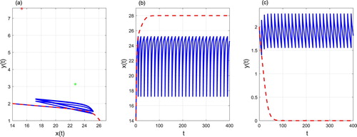
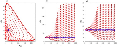
For the case of $x_{ZX}\le x_T\le x_1,$ the phase portrait, time series of prey density and predator density can be seen in Figure 9, where there exists an order-1 periodic solution for $x_T=9.8<x_1=15.2852$ with period $T=\mathrm{8.3333.}$ By Corollary 3.11 the order-1 periodic solution is asymptotically stable.

Figure 9. The phase portrait (a), time series of prey density (b) and predator density (c) starting from $(x_0,y_0)=(15,15)$. Control parameters: $x_{ZX}=30\mathrm{\%}K$, $x_{ZD}=60\mathrm{\%}K$, $x_T=35\mathrm{\%}K=9.8$, $p_T=0.0833$, $q_T=0.0333$ and ${\tau }_T=3.4$. The solution of the free system (1(1) $\begin{array}{rl}& \frac{\mathrm{d}x\left(t\right)}{\mathrm{d}t}=rx\left(t\right)\left(1-\frac{x\left(t\right)}{K}\right)-bx\left(t\right)y\left(t\right),\\ & \frac{\mathrm{d}y\left(t\right)}{\mathrm{d}t}=cx\left(t\right)y\left(t\right)\frac{y\left(t\right)}{y\left(t\right)+m}-\mathrm{d}y\left(t\right).\end{array}$(1) ) is represented in red dotted lines, the solution of the system (3(3) $\left\{\begin{array}{l}\left.\begin{array}{c}\frac{\mathrm{d}x\left(t\right)}{\mathrm{d}t}=rx\left(t\right)\left(1-\frac{x\left(t\right)}{K}\right)-bx\left(t\right)y\left(t\right),\\ \frac{\mathrm{d}y\left(t\right)}{\mathrm{d}t}=cx\left(t\right)y\left(t\right)\frac{y\left(t\right)}{y\left(t\right)+m}-\mathrm{d}y\left(t\right),\end{array}\right\}x<x_T,\\ \left.\begin{array}{c}\mathrm{\Delta }x\left(t\right)=-p\left(x_T\right)x\left(t\right)\\ \mathrm{\Delta }y\left(t\right)=-q\left(x_T\right)y\left(t\right)+\tau \left(x_T\right)\end{array}\right\}x=x_T.\end{array}\right.$(3) ) is presented in blue full line and $E_1$ is represented in red asterisk.

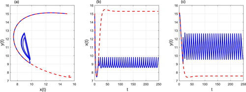
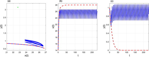
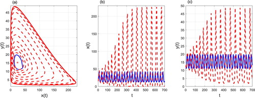
Figure 10 shows the order-1 periodic solution with period T=4.3478 for $x_T=14<x_1=\mathrm{15.2852.}$ Figure 11 shows the phase portrait, time series of prey density and predator density starting from the initial point $(x_0,y_0)=(15,15)$ for $(1-p_T)x_T=10.5875<x_1=15.2852<x_T=\mathrm{15.4.}$ With pest control level $x_T$ increasing, ${\tau }_T$ decreases and the order-1 periodic solution moves from high to low.

Figure 10. The phase portrait (a), time series of prey density (b) and predator density (c) starting from $(x_0,y_0)=(15,15)$. Control parameters: $x_{ZX}=30\mathrm{\%}K$, $x_{ZD}=60\mathrm{\%}K$, $x_T=50\mathrm{\%}K=14$, $p_T=0.3333$, $q_T=0.1333$ and ${\tau }_T=1.6$. The solution of the free system (1(1) $\begin{array}{rl}& \frac{\mathrm{d}x\left(t\right)}{\mathrm{d}t}=rx\left(t\right)\left(1-\frac{x\left(t\right)}{K}\right)-bx\left(t\right)y\left(t\right),\\ & \frac{\mathrm{d}y\left(t\right)}{\mathrm{d}t}=cx\left(t\right)y\left(t\right)\frac{y\left(t\right)}{y\left(t\right)+m}-\mathrm{d}y\left(t\right).\end{array}$(1) ) is represented in red dotted lines, the solution of the system (3(3) $\left\{\begin{array}{l}\left.\begin{array}{c}\frac{\mathrm{d}x\left(t\right)}{\mathrm{d}t}=rx\left(t\right)\left(1-\frac{x\left(t\right)}{K}\right)-bx\left(t\right)y\left(t\right),\\ \frac{\mathrm{d}y\left(t\right)}{\mathrm{d}t}=cx\left(t\right)y\left(t\right)\frac{y\left(t\right)}{y\left(t\right)+m}-\mathrm{d}y\left(t\right),\end{array}\right\}x<x_T,\\ \left.\begin{array}{c}\mathrm{\Delta }x\left(t\right)=-p\left(x_T\right)x\left(t\right)\\ \mathrm{\Delta }y\left(t\right)=-q\left(x_T\right)y\left(t\right)+\tau \left(x_T\right)\end{array}\right\}x=x_T.\end{array}\right.$(3) ) is presented in blue full line and $E_1$ is represented in red asterisk.

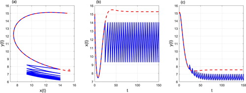
Figure 11. The phase portrait (a), time series of prey density (b) and predator density (c) starting from $(x_0,y_0)=(15,15)$. Control parameters: $x_{ZX}=30\mathrm{\%}K$, $x_{ZD}=60\mathrm{\%}K$, $x_T=55\mathrm{\%}K=15.4$, $p_T=0.4167$, $q_T=0.1667$ and ${\tau }_T=1$. The solution of the free system (1(1) $\begin{array}{rl}& \frac{\mathrm{d}x\left(t\right)}{\mathrm{d}t}=rx\left(t\right)\left(1-\frac{x\left(t\right)}{K}\right)-bx\left(t\right)y\left(t\right),\\ & \frac{\mathrm{d}y\left(t\right)}{\mathrm{d}t}=cx\left(t\right)y\left(t\right)\frac{y\left(t\right)}{y\left(t\right)+m}-\mathrm{d}y\left(t\right).\end{array}$(1) ) is represented in red dotted lines, the solution of the system (3(3) $\left\{\begin{array}{l}\left.\begin{array}{c}\frac{\mathrm{d}x\left(t\right)}{\mathrm{d}t}=rx\left(t\right)\left(1-\frac{x\left(t\right)}{K}\right)-bx\left(t\right)y\left(t\right),\\ \frac{\mathrm{d}y\left(t\right)}{\mathrm{d}t}=cx\left(t\right)y\left(t\right)\frac{y\left(t\right)}{y\left(t\right)+m}-\mathrm{d}y\left(t\right),\end{array}\right\}x<x_T,\\ \left.\begin{array}{c}\mathrm{\Delta }x\left(t\right)=-p\left(x_T\right)x\left(t\right)\\ \mathrm{\Delta }y\left(t\right)=-q\left(x_T\right)y\left(t\right)+\tau \left(x_T\right)\end{array}\right\}x=x_T.\end{array}\right.$(3) ) is presented in blue full line and $E_1$ is represented in red asterisk.

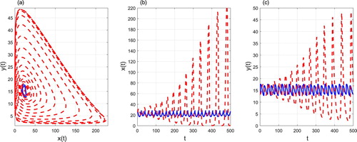
For the case of $x_{ZX}=50\mathrm{\%}K$, $x_{ZD}=95\mathrm{\%}K$, $x_T=90\mathrm{\%}K=25.2$, $(1-p_T)x_T=14.5883<x_1=15.2852<x_2=22.7148<x_T=25.2$ The trajectory starting from the initial point (15,3) tends to an order-1 periodic solution (Figure 12).

Figure 12. The phase portrait (a), time series of prey density (b) and predator density (c) starting from $(x_0,y_0)=(15,3)$. Control parameters: $x_{ZX}=50\mathrm{\%}K$, $x_{ZD}=95\mathrm{\%}K$, $x_T=90\mathrm{\%}K=25.2$, $p_T=0.4211$, $q_T=0.1684$ and ${\tau }_T=0.8$. The solution of the free system (1(1) $\begin{array}{rl}& \frac{\mathrm{d}x\left(t\right)}{\mathrm{d}t}=rx\left(t\right)\left(1-\frac{x\left(t\right)}{K}\right)-bx\left(t\right)y\left(t\right),\\ & \frac{\mathrm{d}y\left(t\right)}{\mathrm{d}t}=cx\left(t\right)y\left(t\right)\frac{y\left(t\right)}{y\left(t\right)+m}-\mathrm{d}y\left(t\right).\end{array}$(1) ) is represented in red dotted lines, the solution of the system (3(3) $\left\{\begin{array}{l}\left.\begin{array}{c}\frac{\mathrm{d}x\left(t\right)}{\mathrm{d}t}=rx\left(t\right)\left(1-\frac{x\left(t\right)}{K}\right)-bx\left(t\right)y\left(t\right),\\ \frac{\mathrm{d}y\left(t\right)}{\mathrm{d}t}=cx\left(t\right)y\left(t\right)\frac{y\left(t\right)}{y\left(t\right)+m}-\mathrm{d}y\left(t\right),\end{array}\right\}x<x_T,\\ \left.\begin{array}{c}\mathrm{\Delta }x\left(t\right)=-p\left(x_T\right)x\left(t\right)\\ \mathrm{\Delta }y\left(t\right)=-q\left(x_T\right)y\left(t\right)+\tau \left(x_T\right)\end{array}\right\}x=x_T.\end{array}\right.$(3) ) is presented in blue full line and $E_1$,$E_2$ are presented in red and green asterisk, respectively.

There is $x_1=15.2852<(1-p_T)x_T=17.2418<x_2=22.7148<x_T=25.2$ when $x_{ZX}=60\mathrm{\%}K$, $x_{ZD}=95\mathrm{\%}K$, $x_T=90\mathrm{\%}K=25.2,$ where an order-1 periodic solution can be seen in Figure 13.

Figure 13. The phase portrait (a), time series of prey density (b) and predator density (c) starting from $(x_0,y_0)=(14,2)$. Control parameters: $x_{ZX}=60\mathrm{\%}K$, $x_{ZD}=95\mathrm{\%}K$, $x_T=90\mathrm{\%}K=25.2$, $p_T=0.3158$, $q_T=0.1263$ and ${\tau }_T=0.9143$. The solution of the free system (1(1) $\begin{array}{rl}& \frac{\mathrm{d}x\left(t\right)}{\mathrm{d}t}=rx\left(t\right)\left(1-\frac{x\left(t\right)}{K}\right)-bx\left(t\right)y\left(t\right),\\ & \frac{\mathrm{d}y\left(t\right)}{\mathrm{d}t}=cx\left(t\right)y\left(t\right)\frac{y\left(t\right)}{y\left(t\right)+m}-\mathrm{d}y\left(t\right).\end{array}$(1) ) is represented in red dotted lines, the solution of the system (3(3) $\left\{\begin{array}{l}\left.\begin{array}{c}\frac{\mathrm{d}x\left(t\right)}{\mathrm{d}t}=rx\left(t\right)\left(1-\frac{x\left(t\right)}{K}\right)-bx\left(t\right)y\left(t\right),\\ \frac{\mathrm{d}y\left(t\right)}{\mathrm{d}t}=cx\left(t\right)y\left(t\right)\frac{y\left(t\right)}{y\left(t\right)+m}-\mathrm{d}y\left(t\right),\end{array}\right\}x<x_T,\\ \left.\begin{array}{c}\mathrm{\Delta }x\left(t\right)=-p\left(x_T\right)x\left(t\right)\\ \mathrm{\Delta }y\left(t\right)=-q\left(x_T\right)y\left(t\right)+\tau \left(x_T\right)\end{array}\right\}x=x_T.\end{array}\right.$(3) ) is presented in blue full line and $E_1$,$E_2$ are presented in red and green asterisk, respectively.

The phase portrait, time series of prey density and predator density can be seen in Figure 14 for $x_{ZX}=85\mathrm{\%}K$, $x_{ZD}=95\mathrm{\%}K$, $x_T=95\mathrm{\%}K=26.6$, and we can get $x_2=22.7148<(1-p_T)x_T=23.799<x_T=\mathrm{26.6.}$

Figure 14. The phase portrait (a), time series of prey density (b) and predator density (c) starting from $(x_0,y_0)=(14,1)$. Control parameters: $x_{ZX}=85\mathrm{\%}K$, $x_{ZD}=95\mathrm{\%}K$, $x_T=95\mathrm{\%}K=26.6$, $p_T=0.1053$, $q_T=0.0421$ and ${\tau }_T=0.4$. The solution of the free system (1(1) $\begin{array}{rl}& \frac{\mathrm{d}x\left(t\right)}{\mathrm{d}t}=rx\left(t\right)\left(1-\frac{x\left(t\right)}{K}\right)-bx\left(t\right)y\left(t\right),\\ & \frac{\mathrm{d}y\left(t\right)}{\mathrm{d}t}=cx\left(t\right)y\left(t\right)\frac{y\left(t\right)}{y\left(t\right)+m}-\mathrm{d}y\left(t\right).\end{array}$(1) ) is represented in red dotted lines, the solution of the system (3(3) $\left\{\begin{array}{l}\left.\begin{array}{c}\frac{\mathrm{d}x\left(t\right)}{\mathrm{d}t}=rx\left(t\right)\left(1-\frac{x\left(t\right)}{K}\right)-bx\left(t\right)y\left(t\right),\\ \frac{\mathrm{d}y\left(t\right)}{\mathrm{d}t}=cx\left(t\right)y\left(t\right)\frac{y\left(t\right)}{y\left(t\right)+m}-\mathrm{d}y\left(t\right),\end{array}\right\}x<x_T,\\ \left.\begin{array}{c}\mathrm{\Delta }x\left(t\right)=-p\left(x_T\right)x\left(t\right)\\ \mathrm{\Delta }y\left(t\right)=-q\left(x_T\right)y\left(t\right)+\tau \left(x_T\right)\end{array}\right\}x=x_T.\end{array}\right.$(3) ) is presented in blue full line and $E_2$ are presented in green asterisk.

Let $r=0.5,c=0.01,b=0.03,d=0.1,m=21.5,K=280.$ then $0<d=0.1<\left(r/2\right)=0.25,K>\left(4r/c\right)=200,m>\left(A_1^2-{\xi }_2^2/A_2\right)=21.4870,Q>0,|m-\left(A_1^2-{\xi }_2^2/A_2\right)|\ll 1.$ We have that the positive equilibrium points are $E_1(24.1158,15.2312)$ and $E_2=(265.8842,0.8402).$ It is easily know from Lemma 3.4 that system (3(3) $\left\{\begin{array}{l}\left.\begin{array}{c}\frac{\mathrm{d}x\left(t\right)}{\mathrm{d}t}=rx\left(t\right)\left(1-\frac{x\left(t\right)}{K}\right)-bx\left(t\right)y\left(t\right),\\ \frac{\mathrm{d}y\left(t\right)}{\mathrm{d}t}=cx\left(t\right)y\left(t\right)\frac{y\left(t\right)}{y\left(t\right)+m}-\mathrm{d}y\left(t\right),\end{array}\right\}x<x_T,\\ \left.\begin{array}{c}\mathrm{\Delta }x\left(t\right)=-p\left(x_T\right)x\left(t\right)\\ \mathrm{\Delta }y\left(t\right)=-q\left(x_T\right)y\left(t\right)+\tau \left(x_T\right)\end{array}\right\}x=x_T.\end{array}\right.$(3) ) has a stable limit cycle. In Figures 14–17, we can find that the system (3(3) $\left\{\begin{array}{l}\left.\begin{array}{c}\frac{\mathrm{d}x\left(t\right)}{\mathrm{d}t}=rx\left(t\right)\left(1-\frac{x\left(t\right)}{K}\right)-bx\left(t\right)y\left(t\right),\\ \frac{\mathrm{d}y\left(t\right)}{\mathrm{d}t}=cx\left(t\right)y\left(t\right)\frac{y\left(t\right)}{y\left(t\right)+m}-\mathrm{d}y\left(t\right),\end{array}\right\}x<x_T,\\ \left.\begin{array}{c}\mathrm{\Delta }x\left(t\right)=-p\left(x_T\right)x\left(t\right)\\ \mathrm{\Delta }y\left(t\right)=-q\left(x_T\right)y\left(t\right)+\tau \left(x_T\right)\end{array}\right\}x=x_T.\end{array}\right.$(3) ) has four kinds of order-1 periodic solution for $h_1<(1-p_T)x_T<x_T<h_2,$ where $S_1(h_1,y_{S_1}),S_2(h_2,y_{S_2})$ are intersect points of the limit cycle and the isoclinic line $\dot{y}=0$ and $h_1<h_2$. Theorem 3.9 only gives the existence of four kinds of order-1 periodic solution for $h_1<(1-p_T)x_T<x_T<h_2$.

Figure 15. The phase portrait (a), time series of prey density (b) and predator density (c) starting from $(x_0,y_0)=(15,13.47)$. Control parameters: $x_{ZX}=1\mathrm{\%}K$, $x_{ZD}=20\mathrm{\%}K$, $x_T=8\mathrm{\%}K=22.4$, $p_T=0.35$, $q_T=0.14$ and ${\tau }_T=8.0211$. The solution of the free system (1(1) $\begin{array}{rl}& \frac{\mathrm{d}x\left(t\right)}{\mathrm{d}t}=rx\left(t\right)\left(1-\frac{x\left(t\right)}{K}\right)-bx\left(t\right)y\left(t\right),\\ & \frac{\mathrm{d}y\left(t\right)}{\mathrm{d}t}=cx\left(t\right)y\left(t\right)\frac{y\left(t\right)}{y\left(t\right)+m}-\mathrm{d}y\left(t\right).\end{array}$(1) ) is represented in red dotted lines, the solution of the system (3(3) $\left\{\begin{array}{l}\left.\begin{array}{c}\frac{\mathrm{d}x\left(t\right)}{\mathrm{d}t}=rx\left(t\right)\left(1-\frac{x\left(t\right)}{K}\right)-bx\left(t\right)y\left(t\right),\\ \frac{\mathrm{d}y\left(t\right)}{\mathrm{d}t}=cx\left(t\right)y\left(t\right)\frac{y\left(t\right)}{y\left(t\right)+m}-\mathrm{d}y\left(t\right),\end{array}\right\}x<x_T,\\ \left.\begin{array}{c}\mathrm{\Delta }x\left(t\right)=-p\left(x_T\right)x\left(t\right)\\ \mathrm{\Delta }y\left(t\right)=-q\left(x_T\right)y\left(t\right)+\tau \left(x_T\right)\end{array}\right\}x=x_T.\end{array}\right.$(3) ) is presented in blue full line and $E_1$ is represented in red asterisk.

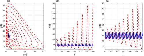
Figure 16. The phase portrait (a), time series of prey density (b) and predator density (c) starting from $(x_0,y_0)=(15.01,15.42)$. Control parameters: $x_{ZX}=1\mathrm{\%}K$, $x_{ZD}=20\mathrm{\%}K$, $x_T=10\mathrm{\%}K=28$, $p_T=0.45$, $q_T=0.18$ and ${\tau }_T=6.8842$. The solution of the free system (1(1) $\begin{array}{rl}& \frac{\mathrm{d}x\left(t\right)}{\mathrm{d}t}=rx\left(t\right)\left(1-\frac{x\left(t\right)}{K}\right)-bx\left(t\right)y\left(t\right),\\ & \frac{\mathrm{d}y\left(t\right)}{\mathrm{d}t}=cx\left(t\right)y\left(t\right)\frac{y\left(t\right)}{y\left(t\right)+m}-\mathrm{d}y\left(t\right).\end{array}$(1) ) is represented in red dotted lines, the solution of the system (3(3) $\left\{\begin{array}{l}\left.\begin{array}{c}\frac{\mathrm{d}x\left(t\right)}{\mathrm{d}t}=rx\left(t\right)\left(1-\frac{x\left(t\right)}{K}\right)-bx\left(t\right)y\left(t\right),\\ \frac{\mathrm{d}y\left(t\right)}{\mathrm{d}t}=cx\left(t\right)y\left(t\right)\frac{y\left(t\right)}{y\left(t\right)+m}-\mathrm{d}y\left(t\right),\end{array}\right\}x<x_T,\\ \left.\begin{array}{c}\mathrm{\Delta }x\left(t\right)=-p\left(x_T\right)x\left(t\right)\\ \mathrm{\Delta }y\left(t\right)=-q\left(x_T\right)y\left(t\right)+\tau \left(x_T\right)\end{array}\right\}x=x_T.\end{array}\right.$(3) ) is presented in blue full line and $E_1$ is represented in red asterisk.

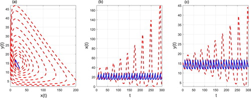
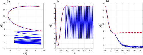
Figure 17. The phase portrait (a), time series of prey density (b) and predator density (c) starting from $(x_0,y_0)=(21.55,16.37)$. Control parameters: $x_{ZX}=1\mathrm{\%}K$, $x_{ZD}=40\mathrm{\%}K$, $x_T=10\mathrm{\%}K=28$, $p_T=0.225$, $q_T=0.09$ and ${\tau }_T=2.7731$. The solution of the free system (1(1) $\begin{array}{rl}& \frac{\mathrm{d}x\left(t\right)}{\mathrm{d}t}=rx\left(t\right)\left(1-\frac{x\left(t\right)}{K}\right)-bx\left(t\right)y\left(t\right),\\ & \frac{\mathrm{d}y\left(t\right)}{\mathrm{d}t}=cx\left(t\right)y\left(t\right)\frac{y\left(t\right)}{y\left(t\right)+m}-\mathrm{d}y\left(t\right).\end{array}$(1) ) is represented in red dotted lines, the solution of the system (3(3) $\left\{\begin{array}{l}\left.\begin{array}{c}\frac{\mathrm{d}x\left(t\right)}{\mathrm{d}t}=rx\left(t\right)\left(1-\frac{x\left(t\right)}{K}\right)-bx\left(t\right)y\left(t\right),\\ \frac{\mathrm{d}y\left(t\right)}{\mathrm{d}t}=cx\left(t\right)y\left(t\right)\frac{y\left(t\right)}{y\left(t\right)+m}-\mathrm{d}y\left(t\right),\end{array}\right\}x<x_T,\\ \left.\begin{array}{c}\mathrm{\Delta }x\left(t\right)=-p\left(x_T\right)x\left(t\right)\\ \mathrm{\Delta }y\left(t\right)=-q\left(x_T\right)y\left(t\right)+\tau \left(x_T\right)\end{array}\right\}x=x_T.\end{array}\right.$(3) ) is presented in blue full line and $E_1$ is represented in red asterisk.

For the case of $x_{ZX}=1\mathrm{\%}K$, $x_{ZD}=20\mathrm{\%}K$,${\tau }_{\max }=12,$ for example $x_T=8\mathrm{\%}K=22.4$, in this case, $h_1<(1-p_T)x_T=18.2<x_T=22.4<x_1=24.1158<h_2,$ there exists an order-1 periodic solution, which is presented in Figure 15. With $x_T$ increasing, i.e. $x_T=10\mathrm{\%}K=28$, an order-1 periodic solution starting from the initial point (15.01,15.42) can be seen in Figure 16 for $h_1<(1-p_T)x_T=15.4<x_1=24.1158<x_T=28<h_2$.

For the case of $x_{ZX}=1\mathrm{\%}K$, $x_{ZD}=40\mathrm{\%}K$, $x_T=10\mathrm{\%}K=28$, ${\tau }_{\max }=3.5,$ the phase portrait, time series of prey density and predator density can be seen in Figure 17, in this case the trajectory starting from (21.55,16.37) tends to an order-1 periodic solution, where $h_1<(1-p_T)x_T=21.7<x_1=24.1158<x_T=28<h_2.$

For the case of $x_{ZX}=10\mathrm{\%}K$, $x_{ZD}=50\mathrm{\%}K$, $x_T=15\mathrm{\%}K=42$, ${\tau }_{\max }=5,$ it can be observed that there exists an order-1 periodic solution from Figure 18, and with a simply calculation, $h_1<x_1=24.1158<(1-p_T)x_T=37.8<x_T=42<h_2.$

Figure 18. The phase portrait (a), time series of prey density (b) and predator density (c) starting from $(x_0,y_0)=(15,13)$. Control parameters: $x_{ZX}=10\mathrm{\%}K$, $x_{ZD}=50\mathrm{\%}K$, $x_T=15\mathrm{\%}K=42$, $p_T=0.1$, $q_T=0.04$ and ${\tau }_T=4.4375$. The solution of the free system (1(1) $\begin{array}{rl}& \frac{\mathrm{d}x\left(t\right)}{\mathrm{d}t}=rx\left(t\right)\left(1-\frac{x\left(t\right)}{K}\right)-bx\left(t\right)y\left(t\right),\\ & \frac{\mathrm{d}y\left(t\right)}{\mathrm{d}t}=cx\left(t\right)y\left(t\right)\frac{y\left(t\right)}{y\left(t\right)+m}-\mathrm{d}y\left(t\right).\end{array}$(1) ) is represented in red dotted lines, the solution of the system (3(3) $\left\{\begin{array}{l}\left.\begin{array}{c}\frac{\mathrm{d}x\left(t\right)}{\mathrm{d}t}=rx\left(t\right)\left(1-\frac{x\left(t\right)}{K}\right)-bx\left(t\right)y\left(t\right),\\ \frac{\mathrm{d}y\left(t\right)}{\mathrm{d}t}=cx\left(t\right)y\left(t\right)\frac{y\left(t\right)}{y\left(t\right)+m}-\mathrm{d}y\left(t\right),\end{array}\right\}x<x_T,\\ \left.\begin{array}{c}\mathrm{\Delta }x\left(t\right)=-p\left(x_T\right)x\left(t\right)\\ \mathrm{\Delta }y\left(t\right)=-q\left(x_T\right)y\left(t\right)+\tau \left(x_T\right)\end{array}\right\}x=x_T.\end{array}\right.$(3) ) is presented in blue full line and $E_1$ is represented in red asterisk.

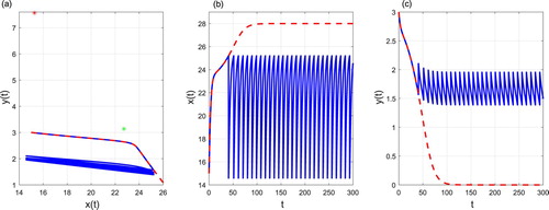
For a suitable selection of parameter values, i.e. $x_{ZX}=5\mathrm{\%}K$, $x_{ZD}=50\mathrm{\%}K$, $x_T=10\mathrm{\%}K=28$, ${\tau }_{\max }=5$, then the existences of order-2 periodic solutions can be seen in Figure 19, which means that the system (3(3) $\left\{\begin{array}{l}\left.\begin{array}{c}\frac{\mathrm{d}x\left(t\right)}{\mathrm{d}t}=rx\left(t\right)\left(1-\frac{x\left(t\right)}{K}\right)-bx\left(t\right)y\left(t\right),\\ \frac{\mathrm{d}y\left(t\right)}{\mathrm{d}t}=cx\left(t\right)y\left(t\right)\frac{y\left(t\right)}{y\left(t\right)+m}-\mathrm{d}y\left(t\right),\end{array}\right\}x<x_T,\\ \left.\begin{array}{c}\mathrm{\Delta }x\left(t\right)=-p\left(x_T\right)x\left(t\right)\\ \mathrm{\Delta }y\left(t\right)=-q\left(x_T\right)y\left(t\right)+\tau \left(x_T\right)\end{array}\right\}x=x_T.\end{array}\right.$(3) ) has complex dynamical behaviours for $h_1<(1-p_T)x_T<x_T<h_2.$

Figure 19. The phase portrait (a), time series of prey density (b) and predator density (c) starting from $(x_0,y_0)=(25,13.4)$. Control parameters: $x_{ZX}=5\mathrm{\%}K$, $x_{ZD}=50\mathrm{\%}K$, $x_T=10\mathrm{\%}K=28$, $p_T=0.1$, $q_T=0.04$ and ${\tau }_T=4.5$. The solution of the free system (1(1) $\begin{array}{rl}& \frac{\mathrm{d}x\left(t\right)}{\mathrm{d}t}=rx\left(t\right)\left(1-\frac{x\left(t\right)}{K}\right)-bx\left(t\right)y\left(t\right),\\ & \frac{\mathrm{d}y\left(t\right)}{\mathrm{d}t}=cx\left(t\right)y\left(t\right)\frac{y\left(t\right)}{y\left(t\right)+m}-\mathrm{d}y\left(t\right).\end{array}$(1) ) is represented in red dotted lines, the solution of the system (3(3) $\left\{\begin{array}{l}\left.\begin{array}{c}\frac{\mathrm{d}x\left(t\right)}{\mathrm{d}t}=rx\left(t\right)\left(1-\frac{x\left(t\right)}{K}\right)-bx\left(t\right)y\left(t\right),\\ \frac{\mathrm{d}y\left(t\right)}{\mathrm{d}t}=cx\left(t\right)y\left(t\right)\frac{y\left(t\right)}{y\left(t\right)+m}-\mathrm{d}y\left(t\right),\end{array}\right\}x<x_T,\\ \left.\begin{array}{c}\mathrm{\Delta }x\left(t\right)=-p\left(x_T\right)x\left(t\right)\\ \mathrm{\Delta }y\left(t\right)=-q\left(x_T\right)y\left(t\right)+\tau \left(x_T\right)\end{array}\right\}x=x_T.\end{array}\right.$(3) ) is presented in blue full line and $E_1$ is represented in red asterisk.

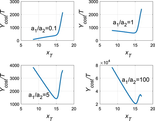
In the case of r=0.5,b=0.03,c=0.01,d=0.1,m=4,K=28, the period T of the order-1 periodic orbit is dependent on the pest control level $x_T$, as shown in Figure 20(a), and the cost per unit time $Y_{\mathrm{cost}}/T$ is presented in Figure 20(b), where the unit cost of the chemical control $a2$ is assumed to be 1000 and the unit cost of culturing the predator $a1$ is 5000. The optimum pest level to take control is $x_T^{\ast }=53.57\mathrm{\%}K=15$, the optimum yield of releases of the predator ${\tau }^{\ast }=3.4172$, the optimum chemical control strength $p^{\ast }=0.3928$ and the optimum frequency of the chemical control is $T^{\ast }=16.6874$. However, it should be noted that the optimum pest level to take control $x_T^{\ast }$ is dependent on the ratio of a1/a2, the larger the ratio a1/a2, the upper the optimum pest level $x_T^{\ast }$, as illustrated in Figure 21.

Figure 20. The change in the order-1 periodic orbit's period T and the cost per unit time $Y_{\mathrm{cost}}/T$ on the pest control level $x_T$ for r=0.5, b=0.03, c=0.01, d=0.1, m=4, K=28.

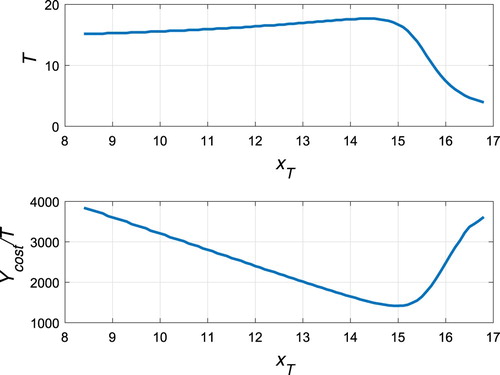
Figure 21. The change in the cost per unit time $Y_{\mathrm{cost}}/T$ on the pest control level $x_T$ for r=0.5, b=0.03, c=0.01, d=0.1, m=4, K=28 with $a1/a2=0.1,1,5,100$.

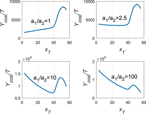
In the case of r=0.5,b=0.03,c=0.01,d=0.1,m=21.5,K=280, the period T of the order-1 periodic orbit is dependent on the pest control level $x_T$, as shown in Figure 22(a), and the cost per unit time $Y_{\mathrm{cost}}/T$ is presented in Figure 22(b), where the unit cost of the chemical control $a2$ is assumed to be 1000 and the unit cost of culturing the predator $a1$ is 10,000. The optimum pest level to take control is $x_T^{\ast }=13.75\mathrm{\%}K=38.5$, the optimum yield of releases of the predator ${\tau }^{\ast }=6.5349$, the optimum chemical control strength $p^{\ast }=0.6375$ and the optimum frequency of the chemical control is $T^{\ast }=14.2625$. However, it should be noted that the optimum pest level to take control $x_T^{\ast }$ is dependent on the ratio of a1/a2, the larger the ratio a1/a2, the upper the optimum pest level $x_T^{\ast }$, as illustrated in Figure 23.

Figure 22. The change in the order-1 periodic orbit's period T and the cost per unit time $Y_{\mathrm{cost}}/T$ on the pest control level $x_T$ for r=0.5, b=0.03, c=0.01, d=0.1, m=21.5, K=280.

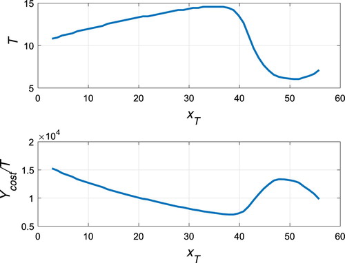
Figure 23. The change in the cost per unit time $Y_{\mathrm{cost}}/T$ on the pest control level $x_T$ for r=0.5, b=0.03, c=0.01, d=0.1, m=21.5, K=280 with $a1/a2=1,2.5,10,100$.

5. Conclusion

In this paper, a predator–prey model with state feedback impulsive control and Allee effect on predator is established and analysed. The results indicate that the existence of order-1 periodic solution (especially homoclinic cycle) for $H_1,H_2$. If $H_3$ holds, the existence of order-k($k\ge 1$) periodic solution is complex. When $h_1<(1-p_T)x_T<x_T<h_2,$ system (3(3) $\left\{\begin{array}{l}\left.\begin{array}{c}\frac{\mathrm{d}x\left(t\right)}{\mathrm{d}t}=rx\left(t\right)\left(1-\frac{x\left(t\right)}{K}\right)-bx\left(t\right)y\left(t\right),\\ \frac{\mathrm{d}y\left(t\right)}{\mathrm{d}t}=cx\left(t\right)y\left(t\right)\frac{y\left(t\right)}{y\left(t\right)+m}-\mathrm{d}y\left(t\right),\end{array}\right\}x<x_T,\\ \left.\begin{array}{c}\mathrm{\Delta }x\left(t\right)=-p\left(x_T\right)x\left(t\right)\\ \mathrm{\Delta }y\left(t\right)=-q\left(x_T\right)y\left(t\right)+\tau \left(x_T\right)\end{array}\right\}x=x_T.\end{array}\right.$(3) ) has at last four kinds of order-1 periodic solutions and order-2 periodic solution. But there exist some troubles in the proof of the existence of order-2 periodic solution, which will be our next work. In order to minimize the control cost, the optimization model is constructed based on the order-1 periodic solution, and the optimal control threshold is obtained by numerical simulation. Simulation results show that the pest control strategy proposed is effective, and the optimal quantity of natural enemies released and the intensity of pesticide sprayed is determined according to the control threshold given by optimization. The state dependent control can be transformed into periodic control, and thus avoid monitoring the population size of the predator.

Disclosure statement

No potential conflict of interest was reported by the authors.

Additional information

Funding

This work is supposed by the National Natural Science Foundation of China [Nos.: 11671346,11371306,11401068], the Project for Science and Technology Open Cooperation of Henan Province [172106000071], Nanhu Scholars Program of XYNU [2016].

References

- K. Baisad and S. Moonchai, Analysis of stability and Hopf bifurcation in a fractional Gauss-type predatorprey model with Allee effect and Holling type-III functional response, Adv. Differ. Eqs. 2018 (2018), p. 82. doi: 10.1186/s13662-018-1535-9
- H.J. Barclay, Models for pest control using predator release habitat management and pesticide release in combination, J. Appl. Ecol. 19 (1982), pp. 337–348. doi: 10.2307/2403471
- W.B. Bian, X. Liu, and J. Geng, Research progress on pests controlling mechanism by natural enemies and its evaluation methods, China Plant Protect. 36 (2016), pp. 17–23.
- E. Bonotto and M. Federson, Limit sets and the poincaré bendixson theorem in impulsive semidynamical systems, J. Differ. Eqs. 244 (2008), pp. 2334–2349. doi: 10.1016/j.jde.2008.02.007
- E. Bonotto and M. Federson, Poisson stability for impulsive semidynamical systems, Nonlinear Anal. 71 (2009), pp. 6148–6156. doi: 10.1016/j.na.2009.06.008
- E. Bonotto and J. Grulha, Lyapunov stability of closed sets in impulsive semidynamical systems, Electron. J. Differential Equations 78 (2010), pp. 1–18.
- G. Buffoni, M. Groppi, and C. Soresina, Dynamics of predatorprey models with a strong Allee effect on the prey and predator-dependent trophic functions, Nonlinear Anal. Real World Appl. 30 (2016), pp. 143–169. doi: 10.1016/j.nonrwa.2015.12.001
- L.S. Chen, Pest control and geometric theory of semi-continuous dynamical system, J. Beihua Univ. 12 (2011), pp. 1–9.
- L.S. Chen, Theory and application of semi-continuous dynamic system, J. Yulin Normal Univ. 34(2) (2012), pp. 2–10.
- X.X. Chen, S.X. Ren, and F. Zhang, Mechanism of pest management by natural enemies and their sustainable utilization, Chin. J. Appl. Entomol. 50 (2013), pp. 9–18.
- F. Courchamp, J. Berec, and J. Gascoigne, Allee Effects in Ecology and Conservation, Oxford University Press, Oxford, New York, 2008.
- H.J. Guo, X.Y. Song, and L.S. Chen, Qualitative analysis of a korean pine forest model with impulsive thinning measure, Appl. Math. Comput. 234 (2014), pp. 203–213.
- G.R. Jiang, Q.S. Lu, and L.N. Qian, Complex dynamics of a Holling type II preypredator system with state feedback control, Chaos Solitons Fractals 31 (2007), pp. 448–461. doi: 10.1016/j.chaos.2005.09.077
- J.J. Jiao and L.S. Chen, Stabilization periodic solution of a state-dependent impulsive single population model subject to Allee effect, Math. Appl. 25 (2012), pp. 413–418.
- D.M. Johnson, A.M. Liebhold, P.C. Tobin, and O.N. Bjrnstad, Allee effects and pulsed invasion by the gypsymoth, Nature 444 (2006), pp. 361–363. doi: 10.1038/nature05242
- D.Flores Jos and Gonzlez-Olivares Eduardo, Dynamics of a predatorprey model with Allee effect on prey and ratio-dependent functional response, Ecol. Complexity 18 (2014), pp. 59–66. doi: 10.1016/j.ecocom.2014.02.005
- A.M. Kramer, B. Dennis, A.M. Liebhold, and J.M. Drake, The evidence for Allee effects, Popul. Ecol. 51 (2009), pp. 341–354. doi: 10.1007/s10144-009-0152-6
- X. Lai, S. Liu, and R. Lin, Rich dynnamical behaviours for predator–prey model with weak Allee effect, Appl. Anal. 89 (2010), pp. 1271–1292. doi: 10.1080/00036811.2010.483557
- X.M. Li and Y. Liao, Study on evaluation of hemiptera predatory insects, J. Anhui Agri. Sci. 39 (2011), pp. 10297–10298.
- L.F. Nie, Z.D. Teng, L Hu, and J.G. Peng, Qualitative analysis of a modified LeslieGower and Holling-type II predatorprey model with state dependent impulsive effects, Nonlinear Anal. Real World Appl. 11 (2010), pp. 1364–1373. doi: 10.1016/j.nonrwa.2009.02.026
- Y.H. Peng and T.H. Zhang, Turing instability and pattern induced by cross-diffusion in a predator–prey system with Allee effect, Appl. Math. Comput. 275 (2016), pp. 1–12.
- R. Peshin and A.K. Dhawan, Integrated Pest Management: Innovation-Development Process, Springer-Verlag, New York, 2009.
- L.N. Qian, Q.S. Lu, Q.G. Meng, and Z.S. Feng, Dynamical behaviors of a preypredator system with impulsive control, J. Math. Anal. Appl. 363 (2010), pp. 345–356. doi: 10.1016/j.jmaa.2009.08.048
- F. Rao and Y. Kang, The complex dynamics of a diffusive preypredator model with an Allee effect in prey, Ecol. Complexity 28 (2016), pp. 123–144. doi: 10.1016/j.ecocom.2016.07.001
- P.S. Simeonov and D.D. Bainov, Orbital stability of periodic solutions of autonomous systems with impulse effect, Int. J. Syst. Sci. 19 (1989), pp. 2561–2585. doi: 10.1080/00207728808547133
- K.B. Sun, T.H. Zhang, and Y. Tian, Theoretical study and control optimization of an integrated pest management predator–prey model with power growth rate, Math. Biosci. 279 (2016), pp. 13–26. doi: 10.1016/j.mbs.2016.06.006
- K.B. Sun, T.H. Zhang, and Y. Tian, Dynamics analysis and control optimization of a pest management predator–prey model with an integrated control strategy, Appl. Math. Comput. 292 (2017), pp. 253–271.
- S.Y. Tang and R.A. Cheke, State-dependent impulsive models of integrated pest management (IPM) strategies and their dynamic consequences, J. Math. Biol. 50 (2005), pp. 257–292. doi: 10.1007/s00285-004-0290-6
- S.Y. Tang and L.S. Chen, Modelling and analysis of integrated pest management strategy, Discrete Contin. Dyn. Syst. Ser. B 4 (2004), pp. 759–768. doi: 10.3934/dcdsb.2004.4.759
- S.Y. Tang, B. Tang, and A.L. Wang, Holling II predator–prey impulsive semi-dynamic model with complex poincaré map, Nonlinear Dyn. 81 (2015), pp. 1–11. doi: 10.1007/s11071-015-1936-1
- S.Y. Tang, Y.N. Xiao, L.S. Chen, and R.A. Cheke, Integrated pest management models and their dynamical behaviour, Bull. Math. Biol. 67 (2005), pp. 115–135. doi: 10.1016/j.bulm.2004.06.005
- S.Y. Tang, Y.N. Xiao, L.S. Chen, and R.A. Cheke, Integrated pest management models and their dynamical behaviour, Bull. Math. Biol. 67 (2010), pp. 115–135. doi: 10.1016/j.bulm.2004.06.005
- Y. Tian, K.B. Sun, and L.S. Chen, Geometric approach to the stability analysis of the periodic solution in a semi-continuous dynamic system, Int. J. Biomath. 7 (2014), pp. 1450018.
- Ünal Ufuktepe, Sinan Kapçak, and Olcay Akman, Stability and invariant manifold for a predator–prey model with Allee effect, Adv Differ. Eqs. 2013 (2013), pp. 348. doi: 10.1186/1687-1847-2013-348
- United Nations, Concise Report on the World Population Situation in 2014, New York, 2014.
- J.C. Van Lenteren, Envirnomental manipulation advantageous to natural enemies of pests, in Integrated Pest Management, V. Delucchi, ed., Parasitis, Geneva, 1987, pp. 123–166.
- J.C. Van Lenteren, Integrated pest management in protected crops, in Integrated Pest Management, D. Dent, ed., Chapman Hall, London, 1995, pp. 311–320.
- J.M. Wang, H.D. Cheng, and X.Z. Meng, Geometrical analysis and control optimization of a predator–prey model with multi state dependent impulse, Adv. Differ. Eqs. 2017 (2017), p. 252. doi: 10.1186/s13662-017-1300-5
- W.M. Wang, Y.N. Zhu, Y.L. Cai, and W.J. Wang, Dynamical complexity induced by Allee effect in a predatorprey model, Nonlinear Anal. Real World Appl. 16 (2014), pp. 103–119. doi: 10.1016/j.nonrwa.2013.09.010
- Y.N. Xiao and F. Van Dan Bosch, The dynamics of an ecoepidemic model with biological control, Ecol. Model. 168 (2003), pp. 203–214. doi: 10.1016/S0304-3800(03)00197-2
- J. Xu, Y. Tian, H. Guo, and X. Song, Dynamical analysis of a pest management LeslieGower model with ratio-dependent functional response, Nonlinear Dyn. 81 (2018), pp. 705–720. doi:10.1007/s11071-018-4219-9
- J. Yang and S.Y. Tang, Holling type II predatorprey model with nonlinear pulse as state-dependent feedback control, J. Comput. Appl. Math. 291 (2016), pp. 225–241. doi: 10.1016/j.cam.2015.01.017
- X.W. Yu, S.L. Yuan, and T.H Zhang, Persistence and ergodicity of a stochastic single species model with Allee effect under regime switching, Commun. Nonlinear Sci. Numer. Simul. 59 (2018), pp. 359–374. doi: 10.1016/j.cnsns.2017.11.028
- T.H. Zhang, X. Liu, X.Z. Meng, and T.Q. Zhang, Spatio-temporal dynnamics near the steady state of a planktonic system, Comput. Math. Appl. 75 (2018), pp. 4490–4504. doi: 10.1016/j.camwa.2018.03.044
- T.Q. Zhang, W.B. Ma, X.Z. Meng, and T.H. Zhang, Periodic solution of a prey-predator model with nonlinear state feedback control, Appl. Math. Comput. 266 (2015), pp. 95–107.
- T.Q. Zhang, W.B. Ma, X.Z. Meng, and Tonghua Zhang, Periodic solution of a preypredator model with nonlinear state feedback control, Appl. Math. Comput. 266 (2015), pp. 95–107.
- T.H. Zhang, T.Q. Zhang, and X.Z. Meng, Spatio-temporal dynamics near the steady state of a planktonic system, Comput. Math. Appl. 75 (2018), pp. 4490–4504. doi: 10.1016/j.camwa.2018.03.044