Stochastic models in seed dispersals: random walks and birth–death processes

ABSTRACT

Seed dispersals deal with complex systems through which the data collected using advanced seed tracking facilities pose challenges to conventional approaches, such as empirical and deterministic models. The use of stochastic models in current seed dispersal studies is encouraged. This review describes three existing stochastic models: the birth–death process (BDP), a 2 dimensional ($2\mathrm{D}$) symmetric random walks and a $2\mathrm{D}$ intermittent walks. The three models possess Markovian property, which make them flexible for studying natural phenomena. Only a few of applications in ecology are found in seed dispersals. The review illustrates how the models are to be used in seed dispersals context. Using the nonlinear BDP, we formulate the individual-based models for two competing plant species while the cover time model is formulated by the symmetric and intermittent random walks. We also show that these three stochastic models can be formulated using the Gillespie algorithm. The full cover time obtained by the symmetric random walks can approximate the Gumbel distribution pattern as the other searching strategies do. We suggest that the applications of these models in seed dispersals may lead to understanding of many complex systems, such as the seed removal experiments and behaviour of foraging agents, among others.

Keywords:

• Birth–death process
• cover time
• individual-based model
• random walk
• seed dispersal

1. Introduction

The seedling survival, growth and development of many plant species depend on seed dispersals through which agents, such as rodents, move seeds away from the seed producing trees. This avoids the intraspecific competition among the seeds when they are many under the parent trees. The agents also benefit from seed dispersals; they often consume the seeds as foods. This mutualistic relationship is a major life-history for the population growth of most plant and animal species [26]. Despite the fact that empirical studies contribute immensely in seed dispersal studies, many complex systems, such as the determination of foraging pattern, could not be understood by field studies alone. This necessitates the use of different approaches, including mathematics, to understand the seed dispersal mechanisms. Even though seed dispersals models exist [41,50], field studies always pose challenges to mathematics due to the emergence of advanced seed tracking facilities. Technology provides many equipment that are currently used for data collection experiments. For over a decade, a motion-sensitive camera trap and radio transmitters have been used to track and monitor the dispersal agents [33].

Therefore, computational ecology develops tools necessary for confronting large amount of data generated through animal tracking facilities [23]. Seed dispersals require effective mathematical tools for understanding and predicting the hidden traits of moving seeds. These tools vary from temporal to spatial models. The choice of an appropriate method depends on many factors, such as the availability of data and managements' objectives, among others [37]. Even if the data are available, it is not always guaranteed to obtain a model that is suitable for the analyses. This compels the application of variety of methods such as individual-based models (IBMs), which their basis entities are individual plants and animals species among others, to seed dispersals. When the real data are not available, IBMs are flexible enough to generate the simulated data. For example, empirical studies of animal movement records the time and location of species in a 50 h plot [68]; nevertheless, sometimes sampling longer distances in forest may be difficult [16]. This problem arises since larger seeds would often dispersed by large animal seed dispersers over thousand metres [57]. Meanwhile, small-bodied frogivores dispersed seeds over a few hundred metres [59]. As Carlo and Morales [12] found that the majority of large-seeded plant species are dispersed by frugivores, such as birds and large animal seed dispersers, which could cover a long distance searching for food. Therefore, the simulated models of animal movements help in understanding and estimating the distances of seeds dispersed by both small and large animal seed dispersers [70]. The survival of regional plant species depends on the long-distance, through which seeds are dispersed by their dispersal agents [65]; mostly large animals.

Even though many IBMs exist in ecological literature, only few of such models have being applied to investigate the dispersal agents' population dynamic and their foraging behaviour. Mathematical models [53,54], mostly formulated deterministically, were applied to study some traits of foraging agents. Applying deterministic models alone will not be enough to understand the characteristics of each individual agent. Considering the random variations, agents move and interact with their potential targets. This, therefore, necessitates the use of stochastic models in seed dispersals. Even though tools [62], such as the birth–death processes (BDPs), symmetric and intermittent random walks, were separately applied in many studies, obtaining a single work that include these three models and relate them to seed dispersals remains elusive. These three models share common Markovian property, through which the future event does not depend on the fast given the present [40]. This review does not serve to replace the existing literature in stochastic modelling, but rather supports and relates them to seed dispersals. By doing this, we hope to promote the applications of these models to investigate different seed dispersal problems. We show that interaction of plant species that require some dispersal agents, time taken by the agent to remove a seed and agents' foraging pattern can all be studied with the three models.

2. Birth–death processes

We consider the BDPs formulated using a continuous-time Markov chain (CTMC), in which the population count of the process is discrete [1]. Using CTMC, a variety of problems are studied. The CTMC of infectious Salman Anemia (a virus infecting fish), for example, was formulated through BDP [46]. In modelling the population growth of a certain species, BDP is often more suitable than the other two forms of this CTMC: pure birth and death processes. In the former, individual is limited to reproduction and no death, while the later allows individual to die young [40]. The advantage of the BDP over these two models can be seen in the waterfowl movement [41], which was formulated to estimate the model parameters. Furthermore, zu Dohna and Pineda-Krch [72] fit the parameters of BDP to infectious disease data. Following this, the BDPs' data were found to fit many probability distributions [44]. In addition, a flexible method for finding transition probabilities of BDPs is determined to handle sophisticated ecological models, whose birth and death transition rates could not be solved analytically [18]. Results obtained by BDPs are often compared with their deterministic analogues. For example, to understand the dynamic of pathogens that spread by wild rodents, both BDPs and their deterministic counterparts were studied, through which some realistic dynamics of rodents' virus were captured [2]. Moreover, BDPs serve as analogue to many well-known differential equations, such as logistic-growth-dispersal model [42], and to some extend they explore changes in demographic stochasticity [39]. Furthermore, BDPs recently approximate fractional differential equations, through which the birth and death rates are linked to regimes: supercritical and under-critical [28]. In infectious disease immunization, the fractional BDP identified the targeted scheme was more efficient than the uniform control [34]. Therefore, BDP is a robust tool for studying seed dispersal problems, such as determining the delay germination of annual organism [38], finding the seed dispersal distance [64] and evaluating the cost (seed predation) and benefit (seed dispersal) of ant-seed dispersals [3]. However, this review found only few of such tools were applied to seed dispersals. We therefore illustrate how the BDP can be used to formulate the IBM of two competing species, which reproduce through seed dispersals process.

2.1. Two species IBM

Capturing the birth, death and behaviour of individual species, the spatio-temporal dynamics is called the IBM [67]. The IBMs are often formulated through BDPs with the aid of Gillespie algorithm [29,30]. These mathematical models [22,45] investigate interaction behaviour between two or more species, such as predation and competition, among others. Therefore, applying interacting populations models in seed dispersals may play important role of understanding mechanisms that structure ecological communities. For example, here we describe how two competing species can be formulated using nonlinear BDP. This illustration may lead to identification of a potential model for understanding mechanisms of seed dispersal, such as the time for each individual species extinction, the effects of different initial population sizes and dispersal rates in two competing species, among others.

Let $N_1\left(t\right)$ and $N_2\left(t\right)$ represent the population counts for two distinct plant species at time t, such that $\left\{N_1\right(t),N_2(t);t\ge 0\}$. Suppose these species compete for limited space and food resources. The probability that the population sizes take the values $n_1,n_2$ can be written as (1) $p(n_1,n_2;t)=p\left[N_1\right(t)=n_1,N_2(t)=n_2],$(1) where $n_1=0,1,2,\dots ,n_2=0,1,2,\dots$. As usual, the formulation of this system begins with stochastic IBMs through which their deterministic counterparts are to be deduced [11]. The schematic reaction of the system can be written as follows:

1. Species $N_1$ and $N_2$ reproduce at (dispersal) rates ${\beta }_1$ and ${\beta }_2$, respectively, such that $N_1⟹{\beta }_{1}2N_1$ and $N_2⟹{\beta }_{2}2N_2$

2. The two plant species $N_1$ and $N_2$ die naturally at (mortality) rates ${\psi }_1$ and ${\psi }_2$ respectively, which results to $N_1⟹{\psi }_1\mathrm{\varnothing }$ and $N_2⟹{\psi }_2\mathrm{\varnothing }$

3. Occupying the same space, the two species interact at (competition) rates ${\alpha }_1$ and ${\alpha }_2$, thereby either $N_1+N_2⟹{\alpha }_{1}2N_1$ or $N_1+N_2⟹{\alpha }_{2}2N_2$.

To obtain the master equation, we list the events occurring in the interval $(t,t+\delta t)$, whereby $\delta t$ is sufficiently small:

1. When nothing has happened, the population was $(n_1,n_2)$ at t, and therefore $1-({\beta }_1{n}_1\delta t+{\beta }_2{n}_2\delta t+{\psi }_1{n}_1\delta t+{\psi }_2{n}_2\delta t+{\alpha }_1{n}_1{n}_2\delta t+{\alpha }_2{n}_1{n}_2\delta t+0\delta t^2)$

2. At time t, the population was $(n_1-1,n_2)$ and $N_1$ reproduced, ${\beta }_1(n_1-1)\delta t+0\delta t^2$

3. At time t, the population was $(n_1,n_2-1)$ and $N_2$ reproduced, ${\beta }_2(n_2-1)\delta t+0\delta t^2$

4. When $N_1$ died naturally, the population at t was $(n_1+1,n_2)$, which results to ${\psi }_1(n_1+1)\delta t+0\delta t^2$

5. The population at t was ($n_1,n_2+1$) when $N_2$ died naturally; ${\psi }_1(n_2+1)\delta t+0\delta t^2$

6. When $N_1$ replaced $N_2$, the population at t was $(n_1-1,n_2+1)$, and it can be written as ${\alpha }_1(n_1-1)(n_2+1)\delta t+0\delta t^2$

7. At t the population was $(n_1+1,n_2-1)$ when $N_2$ replaced $N_1$; ${\alpha }_2(n_1+1)(n_2-1)\delta t+0\delta t^2$.

Summing up the events occurring in the interval $(t,t+\delta t)$ and simplifying the result obtained, the master equation can be written as (2) $\begin{array}{rl}\frac{\mathrm{d}p(n_1,n_2;t)}{\mathrm{d}t}& =-p(n_1,n_2;t)[{\beta }_1{n}_1+{\beta }_2{n}_2+{\psi }_1{n}_1+{\psi }_2{n}_2+{\alpha }_1{n}_1{n}_2+{\alpha }_2{n}_1{n}_2]\\ & +p(n_1-1,n_2;t){\beta }_1(n_1-1)+p(n_1,n_2-1;t){\beta }_2(n_2-1)\\ & +p(n_1+1,n_2;t){\psi }_1(n_1+1)+p(n_1+1,n_2-1;t){\alpha }_2(n_1+1)(n_2-1)\\ & +p(n_1,n_2+1;t){\psi }_2(n_2+1)+p(n_1-1,n_2+1;t){\alpha }_1(n_1-1)(n_2+1).\end{array}$(2) If the process starts with $N_1(n_1,n_2;0)$, $N_2(n_1,n_2;0)$ plant species at time t=0, the initial condition is $p(n_1,n_2;0)=0$ for $n_1\ne n_1\left(0\right)$, $n_2\ne n_2\left(0\right)$, and $p(n_1,n_2;0)=1$ for $n_1=n_1\left(0\right)$, $n_2=n_2\left(0\right)$. The probability for two species stay at $n_1=0$ and $n_2=0$ can be written as (3) $\frac{\mathrm{d}p(0,0;t)}{\mathrm{d}t}=p(1,0;t){\psi }_1\left(1\right)+p(0,1;t){\psi }_2\left(1\right)-p(0,0;t)[{\beta }_1\left(0\right)+{\beta }_2\left(0\right)],$(3) where ${\beta }_1\left(n_1\right),{\beta }_1\left(n_2\right),{\beta }_2\left(n_1\right),{\beta }_2\left(n_2\right)\ge 0$, ${\psi }_1\left(n_1\right),{\psi }_1\left(n_2\right),{\psi }_2\left(n_1\right),{\psi }_2\left(n_2\right)\ge 0$, ${\alpha }_1\left(n_1\right),{\alpha }_1\left(n_2\right),{\alpha }_2\left(n_1\right),{\alpha }_2\left(n_2\right)\ge 0$ for $n_1=0,1,2,\dots$, $n_2=0,1,2,\dots$ and ${\psi }_1\left(0\right)={\psi }_2\left(0\right)={\alpha }_1\left(0\right)={\alpha }_2=0$. When the probability $p(n_1,0;t)$ is considered, the master equation can be written as (4) $\begin{array}{rl}\frac{\mathrm{d}p(n_1,0;t)}{\mathrm{d}t}& =-p(n_1,0;t)[{\beta }_1{n}_1+{\beta }_2\left(0\right)+{\psi }_1{n}_1]+p(n_1-1,0;t){\beta }_1(n_1-1)\\ & +p(n_1+1,0;t){\psi }_1(n_1+1)+p(n_1,1;t){\psi }_2\left(1\right)\\ & +p(n_1-1,1;t){\alpha }_1(n_1-1)\left(1\right),\end{array}$(4) for ${\beta }_2(-1),{\alpha }_2\left(0\right),{\psi }_2\left(0\right)=0$. Meanwhile, the master equation for the other probability $p(0,n_2;t)$ is (5) $\begin{array}{rl}\frac{\mathrm{d}p(0,n_2;t)}{\mathrm{d}t}& =-p(0,n_2;t)[{\beta }_1\left(0\right)+{\beta }_2{n}_2+{\psi }_2{n}_2]+p(0,n_2-1;t){\beta }_2(n_2-1)\\ & +p(1,n_2;t){\psi }_1\left(1\right)+p(1,n_2-1;t){\alpha }_2\left(1\right)(n_2-1)\\ & +p(0,n_2+1;t){\psi }_2(n_2+1),\end{array}$(5) for ${\beta }_1(-1),{\alpha }_1\left(0\right),{\psi }_1\left(0\right)=0$.

In order to solve the master equation  (2(2) $\begin{array}{rl}\frac{\mathrm{d}p(n_1,n_2;t)}{\mathrm{d}t}& =-p(n_1,n_2;t)[{\beta }_1{n}_1+{\beta }_2{n}_2+{\psi }_1{n}_1+{\psi }_2{n}_2+{\alpha }_1{n}_1{n}_2+{\alpha }_2{n}_1{n}_2]\\ & +p(n_1-1,n_2;t){\beta }_1(n_1-1)+p(n_1,n_2-1;t){\beta }_2(n_2-1)\\ & +p(n_1+1,n_2;t){\psi }_1(n_1+1)+p(n_1+1,n_2-1;t){\alpha }_2(n_1+1)(n_2-1)\\ & +p(n_1,n_2+1;t){\psi }_2(n_2+1)+p(n_1-1,n_2+1;t){\alpha }_1(n_1-1)(n_2+1).\end{array}$(2) ), we introduce the probability generating function [19], (6) $F(x,y;t)=\sum _{n_1}^{\mathrm{\infty }}\sum _{n_2}^{\mathrm{\infty }}p(n_1,n_2;t)x^{n_1}{y}^{n_2}.$(6) Differentiating Equation (6(6) $F(x,y;t)=\sum _{n_1}^{\mathrm{\infty }}\sum _{n_2}^{\mathrm{\infty }}p(n_1,n_2;t)x^{n_1}{y}^{n_2}.$(6) ) partially with respect to t and substituting Equation (2(2) $\begin{array}{rl}\frac{\mathrm{d}p(n_1,n_2;t)}{\mathrm{d}t}& =-p(n_1,n_2;t)[{\beta }_1{n}_1+{\beta }_2{n}_2+{\psi }_1{n}_1+{\psi }_2{n}_2+{\alpha }_1{n}_1{n}_2+{\alpha }_2{n}_1{n}_2]\\ & +p(n_1-1,n_2;t){\beta }_1(n_1-1)+p(n_1,n_2-1;t){\beta }_2(n_2-1)\\ & +p(n_1+1,n_2;t){\psi }_1(n_1+1)+p(n_1+1,n_2-1;t){\alpha }_2(n_1+1)(n_2-1)\\ & +p(n_1,n_2+1;t){\psi }_2(n_2+1)+p(n_1-1,n_2+1;t){\alpha }_1(n_1-1)(n_2+1).\end{array}$(2) ) into the result give the following equation: (7) $\begin{array}{rl}\frac{\mathrm{\partial }F(x,y;t)}{\mathrm{\partial }t}& =-{\beta }_1\sum _{n_1}^{\mathrm{\infty }}\sum _{n_2}^{\mathrm{\infty }}{n}_{1}p(n_1,n_2;t)x^{n_1}{y}^{n_2}-{\beta }_2\sum _{n_1}^{\mathrm{\infty }}\sum _{n_2}^{\mathrm{\infty }}{n}_{2}p(n_1,n_2;t)x^{n_1}{y}^{n_2}\\ & -{\psi }_1\sum _{n_1}^{\mathrm{\infty }}\sum _{n_2}^{\mathrm{\infty }}{n}_{1}p(n_1,n_2;t)x^{n_1}{y}^{n_2}-{\psi }_2\sum _{n_1}^{\mathrm{\infty }}\sum _{n_2}^{\mathrm{\infty }}{n}_{2}p(n_1,n_2;t)x^{n_1}{y}^{n_2}\\ & -{\alpha }_1\sum _{n_1}^{\mathrm{\infty }}\sum _{n_2}^{\mathrm{\infty }}{n}_1{n}_{2}p(n_1,n_2;t)x^{n_1}{y}^{n_2}-{\alpha }_2\sum _{n_1}^{\mathrm{\infty }}\sum _{n_2}^{\mathrm{\infty }}{n}_1{n}_{2}p(n_1,n_2;t)x^{n_1}{y}^{n_2}\\ & +{\beta }_1{x}^2\sum _m^{\mathrm{\infty }}\sum _{n_2}^{\mathrm{\infty }}mp(m,n_2;t)x^{m-1}{y}^{n_2}+{\beta }_2{y}^2\sum _{n_1}^{\mathrm{\infty }}\sum _k^{\mathrm{\infty }}kp(n_1,k;t)x^{n_1}{y}^{k-1}\\ & +{\psi }_1\sum _j^{\mathrm{\infty }}\sum _{n_2}^{\mathrm{\infty }}jp(j,n_2;t)x^{j-1}{y}^{n_2}+{\alpha }_2{y}^2\sum _j^{\mathrm{\infty }}\sum _k^{\mathrm{\infty }}jkp(j,k;t)x^{j-1}{y}^{k-1}\\ & +{\psi }_2\sum _{n_1}^{\mathrm{\infty }}\sum _h^{\mathrm{\infty }}hp(n_1,h;t)x^{n_1}{y}^{h-1}+{\alpha }_1{x}^2\sum _m^{\mathrm{\infty }}\sum _h^{\mathrm{\infty }}mhp(m,h;t)x^{m-1}{y}^{h-1},\end{array}$(7) whereby $m=n_1-1$, $j=n_1+1$, $k=n_2-1$, $h=n_2+1$. Simplifying Equation (7(7) $\begin{array}{rl}\frac{\mathrm{\partial }F(x,y;t)}{\mathrm{\partial }t}& =-{\beta }_1\sum _{n_1}^{\mathrm{\infty }}\sum _{n_2}^{\mathrm{\infty }}{n}_{1}p(n_1,n_2;t)x^{n_1}{y}^{n_2}-{\beta }_2\sum _{n_1}^{\mathrm{\infty }}\sum _{n_2}^{\mathrm{\infty }}{n}_{2}p(n_1,n_2;t)x^{n_1}{y}^{n_2}\\ & -{\psi }_1\sum _{n_1}^{\mathrm{\infty }}\sum _{n_2}^{\mathrm{\infty }}{n}_{1}p(n_1,n_2;t)x^{n_1}{y}^{n_2}-{\psi }_2\sum _{n_1}^{\mathrm{\infty }}\sum _{n_2}^{\mathrm{\infty }}{n}_{2}p(n_1,n_2;t)x^{n_1}{y}^{n_2}\\ & -{\alpha }_1\sum _{n_1}^{\mathrm{\infty }}\sum _{n_2}^{\mathrm{\infty }}{n}_1{n}_{2}p(n_1,n_2;t)x^{n_1}{y}^{n_2}-{\alpha }_2\sum _{n_1}^{\mathrm{\infty }}\sum _{n_2}^{\mathrm{\infty }}{n}_1{n}_{2}p(n_1,n_2;t)x^{n_1}{y}^{n_2}\\ & +{\beta }_1{x}^2\sum _m^{\mathrm{\infty }}\sum _{n_2}^{\mathrm{\infty }}mp(m,n_2;t)x^{m-1}{y}^{n_2}+{\beta }_2{y}^2\sum _{n_1}^{\mathrm{\infty }}\sum _k^{\mathrm{\infty }}kp(n_1,k;t)x^{n_1}{y}^{k-1}\\ & +{\psi }_1\sum _j^{\mathrm{\infty }}\sum _{n_2}^{\mathrm{\infty }}jp(j,n_2;t)x^{j-1}{y}^{n_2}+{\alpha }_2{y}^2\sum _j^{\mathrm{\infty }}\sum _k^{\mathrm{\infty }}jkp(j,k;t)x^{j-1}{y}^{k-1}\\ & +{\psi }_2\sum _{n_1}^{\mathrm{\infty }}\sum _h^{\mathrm{\infty }}hp(n_1,h;t)x^{n_1}{y}^{h-1}+{\alpha }_1{x}^2\sum _m^{\mathrm{\infty }}\sum _h^{\mathrm{\infty }}mhp(m,h;t)x^{m-1}{y}^{h-1},\end{array}$(7) ) produces (8) $\begin{array}{rl}\frac{\mathrm{\partial }F(x,y;t)}{\mathrm{\partial }t}& =[{\beta }_{1}x(x-1)-{\psi }_1(x-1)]\frac{\mathrm{\partial }F(x,y;t)}{\mathrm{\partial }x}\\ & +[{\beta }_{2}y(y-1)-{\psi }_2(y-1)]{\beta }_{2}y\frac{\mathrm{\partial }F(x,y;t)}{\mathrm{\partial }y}\\ & +[{\alpha }_{1}x(x-y)-{\alpha }_{2}y(x-y)]\frac{{\mathrm{\partial }}^{2}F(x,y;t)}{\mathrm{\partial }x\mathrm{\partial }y}.\end{array}$(8) Letting $x=e^{\omega }$ and $y=e^{\vartheta }$, we get $M(\omega ,\vartheta ;t)=F(e^{\omega },e^{\vartheta };t)$ [5], which is the moment generating function of the process. Deducing from this change of variables, Equation (8(8) $\begin{array}{rl}\frac{\mathrm{\partial }F(x,y;t)}{\mathrm{\partial }t}& =[{\beta }_{1}x(x-1)-{\psi }_1(x-1)]\frac{\mathrm{\partial }F(x,y;t)}{\mathrm{\partial }x}\\ & +[{\beta }_{2}y(y-1)-{\psi }_2(y-1)]{\beta }_{2}y\frac{\mathrm{\partial }F(x,y;t)}{\mathrm{\partial }y}\\ & +[{\alpha }_{1}x(x-y)-{\alpha }_{2}y(x-y)]\frac{{\mathrm{\partial }}^{2}F(x,y;t)}{\mathrm{\partial }x\mathrm{\partial }y}.\end{array}$(8) ) can be written as (9) $\begin{array}{rl}\frac{\mathrm{\partial }M(\omega ,\vartheta ;t)}{\mathrm{\partial }t}& =[{\beta }_1(e^{\omega }-1)-{\psi }_1(1-e^{-\omega })]\frac{\mathrm{\partial }M(\omega ,\vartheta ;t)}{\mathrm{\partial }\omega }\\ & +[{\beta }_2(e^{\vartheta }-1)-{\psi }_2(1-e^{-\vartheta })]\frac{\mathrm{\partial }M(\omega ,\vartheta ;t)}{\mathrm{\partial }\vartheta }\\ & +[{\alpha }_1(e^{\omega }{e}^{\vartheta }-1)-{\alpha }_2(1-e^{-\omega }{e}^{\vartheta })]\frac{{\mathrm{\partial }}^{2}M(\omega ,\vartheta ;t)}{\mathrm{\partial }\omega \mathrm{\partial }\vartheta }.\end{array}$(9) Using the notation ${\mathrm{\partial }}^{r}M\left(0\right)/\mathrm{\partial }\omega =\mathbb{E}\left(X^r\right)$ [1], we write (10) $\begin{array}{rl}{\left.\frac{\mathrm{\partial }M(\omega ,\vartheta )}{\mathrm{\partial }\omega }\right|}_{\omega =\vartheta =0}& =\mathbb{E}\left(X\right(t\left)\right)\\ {\left.\frac{\mathrm{\partial }M(\omega ,\vartheta )}{\mathrm{\partial }\vartheta }\right|}_{\omega =\vartheta =0}& =\mathbb{E}\left(Y\right(t\left)\right)\\ {\left.\frac{{\mathrm{\partial }}^{2}M(\omega ,\vartheta )}{\mathrm{\partial }\omega \mathrm{\partial }\vartheta }\right|}_{\omega =\vartheta =0}& =\mathbb{E}\left(X\right(t\left)Y\right(t\left)\right).\end{array}$(10) When $\left(\mathrm{\partial }M(\omega ,\vartheta )/\mathrm{\partial }t\right){|}_{\omega =\vartheta =0}$ and substituting Equation (10(10) $\begin{array}{rl}{\left.\frac{\mathrm{\partial }M(\omega ,\vartheta )}{\mathrm{\partial }\omega }\right|}_{\omega =\vartheta =0}& =\mathbb{E}\left(X\right(t\left)\right)\\ {\left.\frac{\mathrm{\partial }M(\omega ,\vartheta )}{\mathrm{\partial }\vartheta }\right|}_{\omega =\vartheta =0}& =\mathbb{E}\left(Y\right(t\left)\right)\\ {\left.\frac{{\mathrm{\partial }}^{2}M(\omega ,\vartheta )}{\mathrm{\partial }\omega \mathrm{\partial }\vartheta }\right|}_{\omega =\vartheta =0}& =\mathbb{E}\left(X\right(t\left)Y\right(t\left)\right).\end{array}$(10) ) into Equation (9(9) $\begin{array}{rl}\frac{\mathrm{\partial }M(\omega ,\vartheta ;t)}{\mathrm{\partial }t}& =[{\beta }_1(e^{\omega }-1)-{\psi }_1(1-e^{-\omega })]\frac{\mathrm{\partial }M(\omega ,\vartheta ;t)}{\mathrm{\partial }\omega }\\ & +[{\beta }_2(e^{\vartheta }-1)-{\psi }_2(1-e^{-\vartheta })]\frac{\mathrm{\partial }M(\omega ,\vartheta ;t)}{\mathrm{\partial }\vartheta }\\ & +[{\alpha }_1(e^{\omega }{e}^{\vartheta }-1)-{\alpha }_2(1-e^{-\omega }{e}^{\vartheta })]\frac{{\mathrm{\partial }}^{2}M(\omega ,\vartheta ;t)}{\mathrm{\partial }\omega \mathrm{\partial }\vartheta }.\end{array}$(9) ), gives (11) $\begin{array}{r}\frac{\mathrm{d}\mathbb{E}\left(X\right(t\left)\right)}{\mathrm{d}t}={\beta }_1\mathbb{E}\left(X\right(t\left)\right)-{\psi }_1\mathbb{E}\left(X\right(t\left)\right)-{\alpha }_2\mathbb{E}\left(X\right(t\left)Y\right(t\left)\right)\end{array}$(11) (12) $\begin{array}{r}\frac{\mathrm{d}\mathbb{E}\left(Y\right(t\left)\right)}{\mathrm{d}t}={\beta }_2\mathbb{E}\left(Y\right(t\left)\right)-{\psi }_2\mathbb{E}\left(Y\right(t\left)\right)-{\alpha }_1\mathbb{E}\left(X\right(t\left)Y\right(t\left)\right).\end{array}$(12) A heuristic approach suggests to substitute Equations (11(11) $\begin{array}{r}\frac{\mathrm{d}\mathbb{E}\left(X\right(t\left)\right)}{\mathrm{d}t}={\beta }_1\mathbb{E}\left(X\right(t\left)\right)-{\psi }_1\mathbb{E}\left(X\right(t\left)\right)-{\alpha }_2\mathbb{E}\left(X\right(t\left)Y\right(t\left)\right)\end{array}$(11) ) and (12(12) $\begin{array}{r}\frac{\mathrm{d}\mathbb{E}\left(Y\right(t\left)\right)}{\mathrm{d}t}={\beta }_2\mathbb{E}\left(Y\right(t\left)\right)-{\psi }_2\mathbb{E}\left(Y\right(t\left)\right)-{\alpha }_1\mathbb{E}\left(X\right(t\left)Y\right(t\left)\right).\end{array}$(12) ) with the corresponding mean field equations of the process, provided by Equations (13(13) $\begin{array}{r}\frac{\mathrm{d}{N}_1\left(t\right)}{\mathrm{d}t}={\beta }_1{N}_1\left(t\right)-{\psi }_1{N}_1\left(t\right)-{\alpha }_2{N}_1\left(t\right)N_2\left(t\right)\end{array}$(13) ) and (14(14) $\begin{array}{r}\frac{\mathrm{d}{N}_2\left(t\right)}{\mathrm{d}t}={\beta }_2{N}_2\left(t\right)-{\psi }_2{N}_2\left(t\right)-{\alpha }_1{N}_1\left(t\right)N_2\left(t\right).\end{array}$(14) ). (13) $\begin{array}{r}\frac{\mathrm{d}{N}_1\left(t\right)}{\mathrm{d}t}={\beta }_1{N}_1\left(t\right)-{\psi }_1{N}_1\left(t\right)-{\alpha }_2{N}_1\left(t\right)N_2\left(t\right)\end{array}$(13) (14) $\begin{array}{r}\frac{\mathrm{d}{N}_2\left(t\right)}{\mathrm{d}t}={\beta }_2{N}_2\left(t\right)-{\psi }_2{N}_2\left(t\right)-{\alpha }_1{N}_1\left(t\right)N_2\left(t\right).\end{array}$(14) Here, Equations (13(13) $\begin{array}{r}\frac{\mathrm{d}{N}_1\left(t\right)}{\mathrm{d}t}={\beta }_1{N}_1\left(t\right)-{\psi }_1{N}_1\left(t\right)-{\alpha }_2{N}_1\left(t\right)N_2\left(t\right)\end{array}$(13) ) and (14(14) $\begin{array}{r}\frac{\mathrm{d}{N}_2\left(t\right)}{\mathrm{d}t}={\beta }_2{N}_2\left(t\right)-{\psi }_2{N}_2\left(t\right)-{\alpha }_1{N}_1\left(t\right)N_2\left(t\right).\end{array}$(14) ) are the deterministic models of the process. The coupled ordinary differential equations appeared in Lotka–Volterra form [6]. Using these equations alone, we cannot be sure of the predictions obtained from the models. The deterministic models lack random variation [20], which is important in studying population dynamics. The variations occur naturally due to fluctuations in birth, death or environmental factors [40]. Therefore, to capture the random variations associated with each individual agent in the two competing species, the computer simulation of the process was formulated. The Gillespie algorithm [29,30], which is efficient in formulating BDPs, was used to build the stochastic IBM. The algorithm uses two random numbers, $r_1$ and $r_2$ that are drown from the uniform distribution. The first random number $r_1$ updates the time in the process. 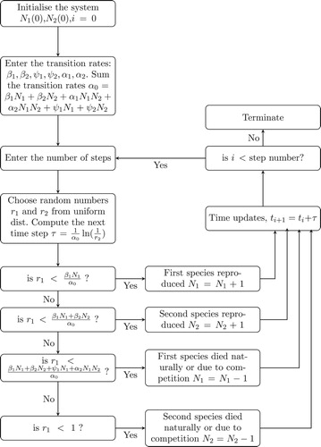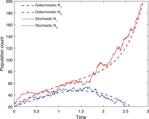Meanwhile, $r_2$ selects the next event, which were given by the transition rates. The whole computer simulation of the two competing species is summarized in the flowchart in Figure 1. After the formulation, the deterministic and stochastic IBMs are usually combined to answer questions that may lead to the understanding of species' coexistence. Though this study is not answering any questions related to the competing species, it combined the two models for the purpose of illustration. In addition, the same arbitrary parameters were used in both deterministic and stochastic IBMs. When observing Figure 2, we notice that the two models are nearly converged. This illustration, therefore, serves as an introduction, which can be modified to study a related seed dispersal problem.

Figure 1. Flowchart for simulating two competing plant species.

3. Random walk models

Random walks theory is among the most widely used models for studying natural phenomena. For more than five decades, the models have been applied in ecology [63] and physics [58], among other related field of studies. Due to the wider scope of random walks, a study [14] discussed the models in detail and identified their applications in biology. In this context, what is considered most among the contributions of random walks is how the models play important role in understanding spatial ecology. Studies conducted on random walks in ecology include how species move [36], where the species can get a target [7], how long it takes the species to find a first target [24]. Other applications of random walks models include the determination of long distance covered by a species [10], finding a foraging patterns of a specie [43,60], prediction of a species perceptual range [61], a distance from which a species detects a target, and estimation of effect of seed dispersals in forest [31]. This review further discusses the regular and irregular random walks: symmetric and intermittent walks. Lacking many applications in seed dispersals, the symmetric and intermittent random walks can be considered as potential tools for understanding dispersal mechanisms. Many agents performing irregular random walks, such as intermittent walks, posses power of locating many targets. However later in this review, we show how the symmetric random walks can approximate the intermittent walks, one of the efficient searching strategies.

Figure 2. The deterministic and stochastic IBMs for two competing plant species $N_1$ and $N_2$ for arbitrary parameters: $N_1\left(0\right)=20$, $N_2\left(0\right)=25$, ${\beta }_1=2$, ${\beta }_2=1.78$, ${\psi }_1=0.02$, ${\psi }_2=0.02$, ${\alpha }_1=0.03$ and ${\alpha }_2=0.03$. The deterministic model is the solution of Equations (13(13) $\begin{array}{r}\frac{\mathrm{d}{N}_1\left(t\right)}{\mathrm{d}t}={\beta }_1{N}_1\left(t\right)-{\psi }_1{N}_1\left(t\right)-{\alpha }_2{N}_1\left(t\right)N_2\left(t\right)\end{array}$(13) ) and (14(14) $\begin{array}{r}\frac{\mathrm{d}{N}_2\left(t\right)}{\mathrm{d}t}={\beta }_2{N}_2\left(t\right)-{\psi }_2{N}_2\left(t\right)-{\alpha }_1{N}_1\left(t\right)N_2\left(t\right).\end{array}$(14) ) while the stochastic simulation is obtained by one realization of the Gillespie algorithm.

3.1. Symmetric random walks

Because the agent has equal chance of moving to any given directions [9], the symmetric walks is considered the simplest form of random walk models. For example in one dimension $1\mathrm{D}$, the agent can move to either left or right with probability of $\frac{1}{2}$ respectively. This can be formulated in the same way with the linear BDP [51]. If δ is the distance covered by the agent in one-step τ, the location of the agent is $(\mu ,{\sigma }^2)\approx (0,\frac{1}{2})$, whereby μ is the mean and ${\sigma }^2$ is the variance. After n-steps of the walks, the location of the agent using the central limit theorem follows the normal distribution, $N(n\mu ,n{\sigma }^2)\approx N(0,n/2)$ [32]. Other important properties of both $1\mathrm{D}$ and $2\mathrm{D}$ symmetric walks, such as the continuum of the models, are discussed in Codling et al. [14] and Allen [1], among other related literature.

Although a $1\mathrm{D}$ symmetric random walks forms the basis for many higher dimensional random walks, a $2\mathrm{D}$ symmetric model is more likely to produce the temporal and spatial patterns associated with the movement of agents. This property, therefore, makes the $2\mathrm{D}$ symmetric walks robust for investigating the movement and foraging of majority of animal seed dispersers [35]. The spatial pattern has influence for the distribution of seeds within a given habitats [69]. 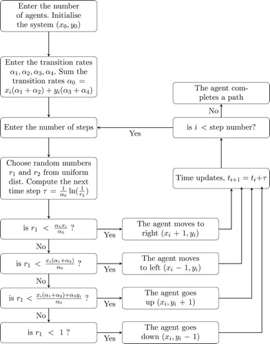As usual, the $2\mathrm{D}$ symmetric can be formulated by the Gillespie algorithm [29,30], and how the computer simulation works is summarized in the flowchart in Figure 3.

Figure 3. Flowchart for the simulation of a $2\mathrm{D}$ symmetric random walks.

3.2. Intermittent random walks

Another random walks described in this review that can be potential for investigating animal seed dispersal problems is the intermittent walks, a model through which an agent performs two different steps with the aid of random numbers. These two steps are called the searching and relocation steps. An agent can switch to a searching step (with a certain rate) if it can thoroughly explore the sites it will visit and alternate to the relocation step (with a relocation rate) if it can lightly visit the sites of a given lattice. The intermittent walks has been used to investigate the foraging behaviour of lizards and fish, among others [56]. Sometimes agents use their cognitive skills to develop more efficient searching strategies, as in the case of human beings looking for jobs or shelter [55].

The whole process of formulating the intermittent random walk is accomplished by implementing the Gillespie algorithm [29,30], as explained earlier. However, we briefly describe it below in relation to our intermittent walks. We chose ρ and ${\mathrm{\Lambda }}_1$ to be our searching and relocation rates respectively. The total rate is given by ${\mathrm{\Lambda }}_0={\mathrm{\Lambda }}_1+\rho$. Therefore, the agent performs a searching step with the probability $\rho /{\mathrm{\Lambda }}_0$ and a relocation step with ${\mathrm{\Lambda }}_1/{\mathrm{\Lambda }}_0$. Note that each of these two probabilities occurs randomly with a random number $r_1$, taken between 0 and 1 from the uniform distribution. If $r_1<\rho /{\mathrm{\Lambda }}_0$, the agent performs a $2\mathrm{D}$ symmetric random walks as described earlier in this section. The time taken after this step increases by $r_2$, which can be written as $t_{i+1}=t_i+r_2$. Whereby $r_2$ is a random number generated from the exponential distribution with the mean value of $1/{\mathrm{\Lambda }}_0$. If the agent performs a relocation step with the probability ${\mathrm{\Lambda }}_1/{\mathrm{\Lambda }}_0$, it navigates randomly to any part of a given lattice with the aid of a random integer R. The time taken to perform this step is the time of the searching steps plus κ, whereby κ is a random number drawn from the exponential distribution with the mean of $1/{\mathrm{\Lambda }}_2$, and ${\mathrm{\Lambda }}_2$ is added to the relocation time: $t_{i+1}=t_i+r_2+\kappa +{\mathrm{\Lambda }}_2$. 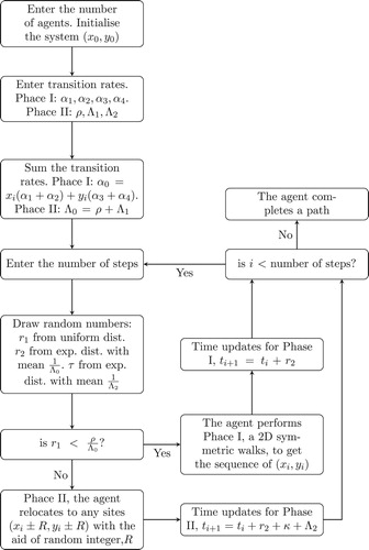This completes one step of the intermittent random walks, and it will continue in this way until the number of steps is exhausted. The flowchart in Figure 4 summarizes the computer simulation for the intermittent walks. Note that a periodic barrier is often used to control the movement of agents at the boundaries.

Figure 4. Flowchart for simulation of a $2\mathrm{D}$ intermittent random walks.

3.3. Cover time models of animal movements

In this section, we describe one application of the random walk models formulated previously. Whenever an agent is moving on a given lattice domain N, the study is interested in two quantities: (i) the number of distinct sites visited by the agent, and (ii) the time taken by the agent to visit the sites. The latter, which is called a cover time, is divided into two: the full $t_f$ and partial $t_p$ cover times. The time taken by an agent to visit all distinct sites of a given lattice is called a full cover time [71]. Meanwhile, if the agent visits only a fraction of the lattice is termed as the partial cover time [17]. Furthermore, the time taken by the agent to reach an absorbing barrier is called the first passage time [66]. One example of this is the simulation model that studied gut-passage time to determine the effects of plant distribution [48]. When many targets are distributed on the lattice domain, averaging their distances from the starting points produces the global mean first passage time of the process $\mathbb{E}\left(\mathrm{T}\right)$ [8].

Cover time problems exist [52,71], but few is applied to other field of studies, such as grand tour that is a statistical tool for describing a multivariate data [4]. Perhaps, the well known results of covering time problems are limited to $1\mathrm{D}$ random walks. This can be seen as in the cases of trapping problems [27,47] and first visit problems [17,21]. Both of these covering time problems are in $1\mathrm{D}$, but if the dimension of cover time problem $\ge 2\mathrm{D}$, the results obtained is hardly to be deduced to any well known random walk problem. Here, the algebra becomes quite involved as the number of dimensions increases; therefore, computing the cover time analytically for dimensions $\ge 2\mathrm{D}$ appears complex [49]. This compels us to formulate our cover time problems numerically using computer simulations. Since the literature on the applications of covering time problem in seed dispersal is lacking, the review shows that a $2\mathrm{D}$ symmetric random walks can be as good as intermittent walks in approximating some covering time problems. Both $2\mathrm{D}$ symmetric and intermittent walks can be good candidates for determining the time taken by animal seed dispersers to encounter seeds and estimating the time costs of foraging species [25], among other related applications.

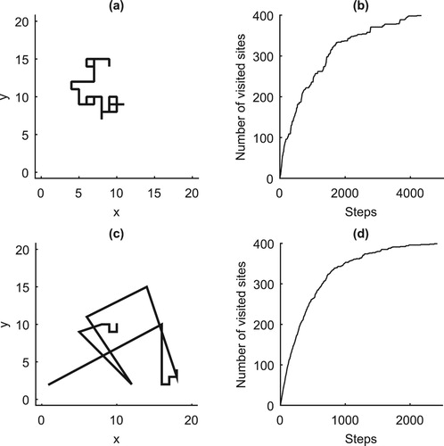
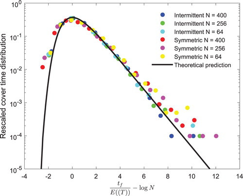
The mean cover time of a $2\mathrm{D}$ random walks, which calculates the time taken by a dispersal agent to cover a given foraging plot, is discussed here. Comparing Figure 5(b,d) shows that the number of steps taken by a symmetric walker to cover a given domain is more than that of the intermittent walker. Though an agent performing symmetric walks may take a longer time to visit a given domain, its cover time distribution converges to that of most irregular random walks, such as the intermittent walks. To find the mean cover time distribution pattern, the $t_f$ is obtained from the random walks, and then $\mathbb{E}\left(\mathrm{T}\right)$ can be determined either asymptotically or numerically from the formulation. After that, $t_f$ is rescaled by the factor, $t_f/\mathbb{E}\left(\mathrm{T}\right)-\log \mathrm{N}$ [13], whereby N is the lattice domain size. Following this, the distribution of the rescaled cover time for both a symmetric and intermittent random walks is given by the Gumbel distribution [13,15] (15) $f\left(x\right)=\frac{1}{v!}\exp (-(v+1)x-e^{-x}),$(15) whereby v is the number of unvisited sites. In order to ascertain the accuracy of the cover time distribution obtained by our symmetric random walks, we adopt the technique used by Chupeau et al. [13], through which Equation (15(15) $f\left(x\right)=\frac{1}{v!}\exp (-(v+1)x-e^{-x}),$(15) ) was used as a theoretical prediction to many irregular random walks.

Figure 5. The paths and mean cover time of a $2\mathrm{D}$ symmetric and a $2\mathrm{D}$ intermittent walks. (a) First 50 steps of a $2\mathrm{D}$ symmetric random walks. (b) An agent, performing a $2\mathrm{D}$ symmetric random walks, takes 4336 steps to visit the domain of N=400. (c) First 20 steps of a $2\mathrm{D}$ intermittent random walks. (d) When performing a $2\mathrm{D}$ intermittent walks, the agent takes 2417 steps to visit N=400.

Furthermore, the distribution of a $2\mathrm{D}$ symmetric and a $2\mathrm{D}$ intermittent walks approximate the Gumbel pattern in many lattice domain sizes, N=64,256,400 (see Figure 6). Even though these domain sizes varied, they approximately collapsed to the theoretical prediction, Equation (15(15) $f\left(x\right)=\frac{1}{v!}\exp (-(v+1)x-e^{-x}),$(15) ). This indicates how the cover time distribution depends on the global mean first passage time of random walks, obtained in periodic domain sizes. All the distributions presented in Figure 6 were obtained when a searcher explored all the sites of a given lattice (v=0).

Figure 6. Cover time distributions for a $2\mathrm{D}$ symmetrical and $2\mathrm{D}$ intermittent walks nearly approximate the Gumbel distribution in different domain sizes for $\rho =20,{\mathrm{\Lambda }}_1=10,{\mathrm{\Lambda }}_2=5$.

4. Conclusion

Seed dispersal is dealing with many complex systems, some of which are difficult to be analysed with empirical or deterministic models alone. Therefore, the review described three stochastic models: BDP, $2\mathrm{D}$ symmetric and intermittent random walks. What makes the formulation of these models encouraging is how they can be formulated through the same Gillespie algorithm, with some slight variations. The models have been applied to study other real world problems. However, their applications in seed dispersals are not many. In an attempt to confront the challenges pose by large amount of data generated from advanced seed tracking facilities, the models and illustrations related to seed dispersals are described in this review. The IBMs for two competing species was taken as an application of BDP. Meanwhile, the cover time problem was introduced to seed dispersals as applications of both the symmetric and intermittent random walks. We have seen that stochastic IBMs approximate their deterministic counterparts. In spatial models, though which the agent performing $2\mathrm{D}$ symmetric walks takes longer time to visit a given domain size; nevertheless, the cover time distribution obtained by the agent converges faster and approximates the distributions obtained by irregular random walks. We suggest that if these three models are to be modified to capture the future of a given seed dispersal (spatial) problem, many important predictions, confronting the challenges of seed tracking data facilities, may be made from the formulation. For example, the complex systems of seed removal process and the agents' foraging behaviour in scatter-hoarding studies can be studied using the described models and illustrations.

Disclosure statement

No potential conflict of interest was reported by the authors.

ORCID

S. Shohaimi  http://orcid.org/0000-0003-0591-6627

A. Kilicman  http://orcid.org/0000-0002-1217-963X

Additional information

Funding

This work is supported by the Geran Putra IPS, Project number: GP-IPs/2018/9657400.

References

- L.J. Allen, An Introduction to Stochastic Processes with Applications to Biology, CRC Press, Boca Raton, 2010.
- L.J. Allen, R.K. McCormack, and C.B. Jonsson, Mathematical models for hantavirus infection in rodents, Bull. Math. Biol. 68 (2006), pp. 511–524 doi: 10.1007/s11538-005-9034-4
- X. Arnan, R. Molowny-Horas, A. Rodrigo, and J. Retana, Uncoupling the effects of seed predation and seed dispersal by granivorous ants on plant population dynamics, PLoS One 7 (2012), pp. e42869. doi: 10.1371/journal.pone.0042869
- D. Asimov, The grand tour: A tool for viewing multidimensional data, SIAM J. Sci. Stat. Comput. 6 (1985), pp. 128–143. doi: 10.1137/0906011
- N.T. Bailey, The Elements of Stochastic Processes with Applications to the Natural Sciences, John Wiley & Sons, New York, 1990. Vol. 25.
- B. Barnes, G.R. Fulford, Mathematical Modelling with Case Studies: Using Maple and Matlab, CRC Press, Boca Raton, 2014. Vol. 25.
- F. Bartumeus, M.E. Da Luz, G. Viswanathan, and J. Catalan, Animal search strategies: A quantitative random-walk analysis, Ecology 86 (2005), pp. 3078–3087. doi: 10.1890/04-1806
- O. Bénichou and R. Voituriez, From first-passage times of random walks in confinement to geometry-controlled kinetics, Phys. Rep. 539 (2014), pp. 225–284. doi: 10.1016/j.physrep.2014.02.003
- H.C. Berg, Random Walks in Biology, Princeton University Press, Princeton, 1993.
- C.M. Bergman, J.A. Schaefer, and S. Luttich, Caribou movement as a correlated random walk, Oecologia 123 (2000), pp. 364–374. doi: 10.1007/s004420051023
- A.J. Black and A.J. McKane, Stochastic formulation of ecological models and their applications, Trends Ecol. Evol. 27 (2012), pp. 337–345. doi: 10.1016/j.tree.2012.01.014
- T.A. Carlo and J.M. Morales, Inequalities in fruit-removal and seed dispersal: Consequences of bird behaviour, neighbourhood density and landscape aggregation, J. Ecol. 96 (2008), pp. 609–618. doi: 10.1111/j.1365-2745.2008.01379.x
- M. Chupeau, O. Bénichou, and R. Voituriez, Cover times of random searches, Nat. Phys. 11 (2015), pp. 844–847 doi: 10.1038/nphys3413
- E.A. Codling, M.J. Plank, and S. Benhamou, Random walk models in biology, J. Royal Soc. Interface 5 (2008), pp. 813–834. doi: 10.1098/rsif.2008.0014
- S. Coles, J. Bawa, L. Trenner, An Introduction to Statistical Modeling of Extreme Values, Springer, London, 2001. Vol. 208.
- M.C. Côrtes and M. Uriarte, Integrating frugivory and animal movement: A review of the evidence and implications for scaling seed dispersal, Biol. Rev. 88 (2013), pp. 255–272. doi: 10.1111/j.1469-185X.2012.00250.x
- K. Coutinho, M. Coutinho-Filho, M. Gomes, and A. Nemirovsky, Partial and random lattice covering times in two dimensions, Phys. Rev. Lett. 72 (1994), pp. 3745–3749 doi: 10.1103/PhysRevLett.72.3745
- F.W. Crawford and M.A. Suchard, Transition probabilities for general birth–death processes with applications in ecology, genetics, and evolution, J. Math. Biol. 65 (2012), pp. 553–580. doi: 10.1007/s00285-011-0471-z
- A.D. Crescenzo and B. Martinucci, A first-passage-time problem for symmetric and similar two-dimensional birth–death processes, Stoch. Models 24 (2008), pp. 451–469. doi: 10.1080/15326340802232293
- D.L. DeAngelis and W.M. Mooij, Individual-based modeling of ecological and evolutionary processes, Annu. Rev. Ecol. Evol. Syst. 36 (2005), pp. 147–168. doi: 10.1146/annurev.ecolsys.36.102003.152644
- A. Dembo, Y. Peres, J. Rosen, Cover times for brownian motion and random walks in two dimensions. Ann. Math. 160 (2004), pp. 433–464. doi: 10.4007/annals.2004.160.433
- R. Erban, J. Chapman, and P. Maini, A practical guide to stochastic simulations of reaction-diffusion processes, 2007. arXiv preprint arXiv:0704.1908.
- W.F. Fagan, M.A. Lewis, M. Auger-Méthé, T. Avgar, S. Benhamou, G. Breed, L. LaDage, U.E. Schlägel, W.W. Tang, Y.P. Papastamatiou, J. Forester, T. Mueller, and J. Clobert, Spatial memory and animal movement, Ecol. Lett. 16 (2013), pp. 1316–1329. doi: 10.1111/ele.12165
- P. Fauchald and T. Tveraa, Using first-passage time in the analysis of area-restricted search and habitat selection, Ecology 84 (2003), pp. 282–288. doi: 10.1890/0012-9658(2003)084[0282:UFPTIT]2.0.CO;2
- J.H. Fewell, Energetic and time costs of foraging in harvester ants, pogonomyrmex occidentalis, Behav. Ecol. Sociobiol. 22 (1988), pp. 401–408. doi: 10.1007/BF00294977
- E.A. Fronhofer, E.B. Sperr, A. Kreis, M. Ayasse, H.J. Poethke, and M. Tschapka, Picky hitch-hikers: Vector choice leads to directed dispersal and fat-tailed kernels in a passively dispersing mite, Oikos 122 (2013), pp. 1254–1264. doi: 10.1111/j.1600-0706.2013.00503.x
- L.K. Gallos, Random walk and trapping processes on scale-free networks, Phys. Rev. E 70 (2004), p. 046116. doi: 10.1103/PhysRevE.70.046116
- R. Garra and F. Polito, A note on fractional linear pure birth and pure death processes in epidemic models, Phys. A Stat. Mech. Appl. 390 (2011), pp. 3704–3709. doi: 10.1016/j.physa.2011.06.005
- D.T. Gillespie, A general method for numerically simulating the stochastic time evolution of coupled chemical reactions, J. Comput. Phys. 22 (1976), pp. 403–434. doi: 10.1016/0021-9991(76)90041-3
- D.T. Gillespie, Exact stochastic simulation of coupled chemical reactions, J. Phys. Chem. 81 (1977), pp. 2340–2361. doi: 10.1021/j100540a008
- D.G. Green, Simulated effects of fire, dispersal and spatial pattern on competition within forest mosaics, Vegetatio 82 (1989), pp. 139–153. doi: 10.1007/BF00045027
- G. Grimmett, D. Stirzaker, Probability and Random Processes, Oxford University Press, Oxford, 2001.
- B.T. Hirsch, R. Kays, and P.A. Jansen, A telemetric thread tag for tracking seed dispersal by scatter-hoarding rodents, Plant Ecol. 213 (2012), pp. 933–943. doi: 10.1007/s11258-012-0054-0
- J. Huo and H. Zhao, Dynamical analysis of a fractional sir model with birth and death on heterogeneous complex networks, Physica A Stat. Mech. Appl. 448 (2016), pp. 41–56. doi: 10.1016/j.physa.2015.12.078
- O.C. Ibe, Two-dimensional random walk, in Elements of Random Walk and Diffusion Processes, 2013, pp. 103–128.
- D.S. Johnson, J.M. London, M.A. Lea, and J.W. Durban, Continuous-time correlated random walk model for animal telemetry data, Ecology 89 (2008), pp. 1208–1215. doi: 10.1890/07-1032.1
- E. Jongejans, O. Skarpaas, and K. Shea, Dispersal, demography and spatial population models for conservation and control management, Perspect. Plant Ecol. Evol. Syst. 9 (2008), pp. 153–170. doi: 10.1016/j.ppees.2007.09.005
- P. Klinkhamer, T. De Jong, J. Metz, and J. Val, Life history tactics of annual organisms: The joint effects of dispersal and delayed germination, Theor. Popul. Biol. 32 (1987), pp. 127–156. doi: 10.1016/0040-5809(87)90044-X
- A. Kolpas and R.M. Nisbet, Effects of demographic stochasticity on population persistence in advective media, Bull. Math. Biol. 72 (2010), pp. 1254–1270. doi: 10.1007/s11538-009-9489-4
- M. Kot, Elements of Mathematical Ecology, Cambridge University Press, Cambridge, 2001.
- M. Kot, M.A. Lewis, and P. van den Driessche, Dispersal data and the spread of invading organisms, Ecology 77 (1996), pp. 2027–2042. doi: 10.2307/2265698
- F. Lutscher, E. Pachepsky, and M.A. Lewis, The effect of dispersal patterns on stream populations, SIAM Rev. 47 (2005), pp. 749–772. doi: 10.1137/050636152
- A. Mårell, J.P. Ball, and A. Hofgaard, Foraging and movement paths of female reindeer: Insights from fractal analysis, correlated random walks, and lévy flights, Can. J. Zool. 80 (2002), pp. 854–865. doi: 10.1139/z02-061
- Y.E. Maruvka, D.A. Kessler, and N.M. Shnerb, The birth–death–mutation process: A new paradigm for fat tailed distributions, PLoS One 6 (2011), p. e26480. doi: 10.1371/journal.pone.0026480
- A.J. McKane and T.J. Newman, Predator-prey cycles from resonant amplification of demographic stochasticity, Phys. Rev. Lett. 94 (2005), p. 218102. doi: 10.1103/PhysRevLett.94.218102
- E. Milliken, The probability of extinction of infectious salmon anemia virus in one and two patches, Bull. Math. Biol. 79 (2017), pp. 2887–2904. doi: 10.1007/s11538-017-0355-5
- E.W. Montroll, Random walks on lattices containing traps, in Physical Society of Japan Journal Supplement, Vol. 26. Proceedings of the International Conference on Statistical Mechanics held 9–14 September, 1968 in Koyto, 1969, p. 6.
- J.M. Morales and T.A. Carlo, The effects of plant distribution and frugivore density on the scale and shape of dispersal kernels, Ecology 87 (2006), pp. 1489–1496. doi: 10.1890/0012-9658(2006)87[1489:TEOPDA]2.0.CO;2
- M.S. Nascimento, M.D. Coutinho-Filho, and C.S. Yokoi, Partial and random covering times in one dimension, Phys. Rev. E 63 (2001), pp. 066125. doi: 10.1103/PhysRevE.63.066125
- R. Nathan, G.G. Katul, H.S. Horn, S.M. Thomas, R. Oren, R. Avissar, S.W. Pacala, and S.A. Levin, Mechanisms of long-distance dispersal of seeds by wind, Nature 418 (2002), pp. 409–413 doi: 10.1038/nature00844
- S. Nee, Birth–death models in macroevolution, Annu. Rev. Ecol. Evol. Syst. 37 (2006), pp. 1–17. doi: 10.1146/annurev.ecolsys.37.091305.110035
- A.M. Nemirovsky and M.D. Coutinho-Filho, Lattice covering time in d dimensions: Theory and mean field approximation, Physica A Stat. Mech. Appl. 177 (1991), pp. 233–240. doi: 10.1016/0378-4371(91)90158-9
- M.G. Neubert and H. Caswell, Demography and dispersal: Calculation and sensitivity analysis of invasion speed for structured populations, Ecology 81 (2000), pp. 1613–1628. doi: 10.1890/0012-9658(2000)081[1613:DADCAS]2.0.CO;2
- M.G. Neubert, M. Kot, and M.A. Lewis, Dispersal and pattern formation in a discrete-time predator-prey model, Theor. Popul. Biol. 48 (1995), pp. 7–43. doi: 10.1006/tpbi.1995.1020
- G. Oshanin, K. Lindenberg, H.S. Wio, and S. Burlatsky, Efficient search by optimized intermittent random walks, J. Phys. A Math. Theor. 42 (2009), p. 434008. doi: 10.1088/1751-8113/42/43/434008
- G. Oshanin, H. Wio, K. Lindenberg, and S. Burlatsky, Intermittent random walks for an optimal search strategy: One-dimensional case, J. Phys. Condens. Matt. 19 (2007), p. 065142. doi: 10.1088/0953-8984/19/6/065142
- R. Pakeman, Plant migration rates and seed dispersal mechanisms, J. Biogeogr. 28 (2001), pp. 795–800. doi: 10.1046/j.1365-2699.2001.00581.x
- C.S. Patlak, Random walk with persistence and external bias, Bull. Math. Biophys. 15 (1953), pp. 311–338. doi: 10.1007/BF02476407
- M.M. Pires, P.R. Guimarães, M. Galetti, and P. Jordano, Pleistocene megafaunal extinctions and the functional loss of long-distance seed-dispersal services, Ecography 41 (2018), pp. 153–163. doi: 10.1111/ecog.03163
- G. Ramos-Fernández, J.L. Mateos, O. Miramontes, G. Cocho, H. Larralde, and B. Ayala-Orozco, Lévy walk patterns in the foraging movements of spider monkeys (ateles geoffroyi), Behav. Ecol. Sociobiol. 55 (2004), pp. 223–230. doi: 10.1007/s00265-003-0700-6
- R.L. Schooley and J.A. Wiens, Finding habitat patches and directional connectivity, Oikos 102 (2003), pp. 559–570. doi: 10.1034/j.1600-0706.2003.12490.x
- L.D. Servi, Algorithmic solutions to two-dimensional birth–death processes with application to capacity planning, Telecommun. Syst. 21 (2002), pp. 205–212. doi: 10.1023/A:1020942430425
- J.G. Skellam, Random dispersal in theoretical populations, Biometrika 38 (1951), pp. 196–218. doi: 10.1093/biomet/38.1-2.196
- M.B. Soons, G.W. Heil, R. Nathan, and G.G. Katul, Determinants of long-distance seed dispersal by wind in grasslands, Ecology 85 (2004), pp. 3056–3068. doi: 10.1890/03-0522
- M.B. Soons and W.A. Ozinga, How important is long-distance seed dispersal for the regional survival of plant species? Divers. Distrib. 11 (2005), pp. 165–172. doi: 10.1111/j.1366-9516.2005.00148.x
- U. Sumita and Y. Masuda, On first passage time structure of random walks, Stoch. Process. Their Appl. 20 (1985), pp. 133–147. doi: 10.1016/0304-4149(85)90021-3
- N. Tkachenko, J.D. Weissmann, W.P. Petersen, G. Lake, C.P. Zollikofer, and S. Callegari, Individual-based modelling of population growth and diffusion in discrete time, PLoS One 12 (2017), p. e0176101. doi: 10.1371/journal.pone.0176101
- E.V. Wehncke, S.P. Hubbell, R.B. Foster, and J.W. Dalling, Seed dispersal patterns produced by white-faced monkeys: Implications for the dispersal limitation of neotropical tree species, J. Ecol. 91 (2003), pp. 677–685. doi: 10.1046/j.1365-2745.2003.00798.x
- D.A. Westcott and D.L. Graham, Patterns of movement and seed dispersal of a tropical frugivore, Oecologia 122 (2000), pp. 249–257. doi: 10.1007/PL00008853
- H. Will and O. Tackenberg, A mechanistic simulation model of seed dispersal by animals, J. Ecol. 96 (2008), pp. 1011–1022. doi: 10.1111/j.1365-2745.2007.01341.x
- C.S. Yokoi, A. Hernández-Machado, and L. Ramírez-Piscina, Some exact results for the lattice covering time problem, Phys. Lett. A 145 (1990), pp. 82–86. doi: 10.1016/0375-9601(90)90196-U
- H. zu Dohna and M. Pineda-Krch, Fitting parameters of stochastic birth–death models to metapopulation data, Theor. Popul. Biol. 78 (2010), pp. 71–76. doi: 10.1016/j.tpb.2010.06.004