Optimal control of a vectored plant disease model for a crop with continuous replanting

ABSTRACT

Vector-transmitted diseases of plants have had devastating effects on agricultural production worldwide, resulting in drastic reductions in yield for crops such as cotton, soybean, tomato, and cassava. Plant-vector-virus models with continuous replanting are investigated in terms of the effects of selection of cuttings, roguing, and insecticide use on disease prevalence in plants. Previous models are extended to include two replanting strategies: frequencyreplanting and abundance-replanting. In frequency-replanting, replanting of infected cuttings depends on the selection frequency parameter ε, whereas in abundance-replanting, replanting depends on plant abundance via a selection rate parameter also denoted as ε. The two models are analysed and new thresholds for disease elimination are defined for each model. Parameter values for cassava, whiteflies, and African cassava mosaic virus serve as a case study. A numerical sensitivity analysis illustrates how the equilibrium densities of healthy and infected plants vary with parameter values. Optimal control theory is used to investigate the effects of roguing and insecticide use with a goal of maximizing the healthy plants that are harvested. Differences in the control strategies in the two models are seen for large values of ε. Also, the combined strategy of roguing and insecticide use performs better than a single control.

KEYWORDS:

• Vectored plant disease
• replanting strategies
• optimal control
• differential equations

1. Introduction

Insect transmission of plant diseases is an important source of agricultural infestation. Begomoviruses, carried by the whitefly Bemisia tabaci, are some of the most important emerging viral pathogens of crops [27,28]. These viruses have caused drastic reductions in productivity for crops such as cotton, soybean, tomato, and cassava [27,28]. African cassava mosaic virus (ACMV) is transmitted to cassava plants by the whitefly B. tabaci which results in African cassava mosaic disease (ACMD). Cassava mosaic viruses are found in Africa, India, and Sri Lanka [2]. Annual tuber loss from cassava mosaic disease in sub-Saharan Africa has been estimated as 15–24% [2]. Management strategies for ACMD include control of the whitefly vector and roguing (removal of infected plants). Generally, control of vectors by insecticides is considered less effective in comparison to other control methods which include roguing, selection of healthy stem cuttings, and planting of resistant varieties [2,8,23].

Mathematical models of plant–virus and plant–vector–virus models have provided insight into effective methods for reduction of disease incidence and for increase in plant productivity (e.g.[5,6,10,11,13–15,24,29,35]). Several plant–vector–virus models have been specifically applied to ACMV (e.g.[11,14,15,35]). Roguing of infected plants is one strategy that is used to control the spread of plant viral diseases. Identification of latent diseased plants is one of the key issues for effective control, where the diseased plants are removed from the field, a cultural control method called roguing. Roguing, combined with replanting of healthy material, is a common field practice. Time-dependent models have been proposed to evaluate whether eradication is feasible [5]. In general, much of the modeling work has been theoretical, in an attempt to determine what needs to be done to achieve a given level of disease control. These theoretical analyses are similar to the research in human epidemiology which studies the impact of population vaccination programs.

The effect of roguing has been investigated in several plant–virus and plant–vector–virus models [5,10,13–15,24]. In the plant–virus model of Chan and Jeger [5], roguing is sensitive to the contact rate between susceptible and infectious hosts. At low contact rates, roguing of infectious plants is effective, but at high contact rates effective control requires roguing of both infectious and latent plants [5]. In another plant–virus model by Gao et al. [10], roguing was implemented through periodic removal. Similar results were obtained as in Chan and Jeger [5], except in [10], it was noted that continuous control may overestimate infectious risk as compared to impulsive control.

A range of control options has been used against cassava mosaic disease (CMD) in sub-Saharan Africa with the greatest emphasis on the development and deployment of virus resistant varieties. Much less emphasis has been placed on sanitation measures, such as roguing or the use of inter-cropping [31]. Large-scale screening of cassava for resistance to B. tabaci emphasized the levels of whitefly infestation and preferential whitefly visitation at different locations in Nigeria [4]. A comparison of CMD and cassava brown streak disease pandemics in E. Africa [19] showed different patterns of symptom expression indicating that the effectiveness of phytosanitation methods differs. The temporal relationship between vector abundance and disease incidence highlighted the urgent need to implement vector control strategies.

In a recent model by Hilker et al. [13], a complex model based on cropping seasons was specifically developed for study of maize lethal necrosis, a plant disease caused by coinfection with two viruses. Vectors were not explicitly modelled. However, as the viruses may be transmitted via vector, soil, and seed, several control methods were studied including use of clean seed, implicit control of vectors, crop rotation, and roguing. It was found that when clean seeds are limited, crop rotation and roguing are the most effective strategies. In a plant–vector–virus model for crops replanted from stem cuttings and continuous harvesting, Holt et al. [14] and Jeger et al. [15] showed that roguing has only a slight impact on disease incidence while an increase in healthy plants prevents total infection. The recent model of McQuaid et al. [24] includes the effect of grower behavior on disease incidence. One interesting result of the model analysis showed that growers adoption of particular control strategies can result in cycles of disease incidence.

More theoretical mathematical analyses of plant models have studied global stability of endemic states and the effect of generic roguing/replanting strategies [6,21,29,32]. In [6], an SEI epidemic model of plant viral diseases incorporating disease latency, roguing, and constant recruitment in both the healthy and infected plants is analyzed. In [29], a plant–vector virus model is analysed that incorporates infection of healthy plants by infective vectors or by infected plants.

In this investigation, we consider two plant–vector–virus models applied to a vegetatively propagated crop with continuous replanting from cuttings harvested within the field. In general, replanting may include cuttings from both healthy and infected plants. The first model was formulated by Holt et al. [14] and Jeger et al. [15] in which replanting is based on a selection frequency of infected plants. We call this replanting strategy frequency-replanting. The second model, formulated in the next section, makes a different assumption about replanting, based on total plant abundance in the field via a selection rate parameter. We call this new replanting strategy abundance-replanting. With density-dependent replacement rate, it is shown that the two models differ in the rate of replacement. When selection of infected cuttings is high, then the replacement rate is slower in frequency-replanting than in abundance-replanting. However, in both models, the total plant abundance is reduced with infected plants.

The two models (frequency and abundance) are applied to a case study of African cassava mosaic virus (ACMV), as in [14,15]. We compare the two models with respect to replanting strategies through a combination of mathematical analysis, parameter sensitivity analysis, and optimal control of the disease dynamics. For both models, thresholds for disease eradication are defined, the basic and type reproduction numbers. A numerical investigation of parameter sensitivity of the equilibrium values is performed. For a fixed selection frequency or rate, optimal control theory is used to investigate the effect of roguing and insecticide use (vector control), with the objective to maximize a combination of the healthy plants harvested at the final time (end of season) and the discounted stream of revenue from harvesting tubers from cassava plants less the cost of implementing the two controls. Several disease control scenarios are investigated, including either only roguing or only insecticide use and both roguing and insecticide use.

Mathematical studies of optimal control applied to other vectored plant diseases have also been considered, see for example [1,34]. In [34], Venturino et al. consider a model for mosaic virus disease in a plant called Jatropha curcas. Mathematical analysis and optimal control are applied to study the disease using insecticide spray that reduces the transmission rates between the vector and host. In [1], Al Basir et al. extend the model and the analysis from [34] to include roguing of infected plants. Neither model includes harvesting or replanting strategies. The effect of replanting strategies on plant dynamics is one of the main aims of this paper. In addition to construction of a new model for a replanting strategy, and comparison of the two replanting strategies, other distinct features of our models include harvesting of both healthy and infected plants, and separation of natural death of vectors from death due to insecticide application. Our optimal control problem includes insecticide spray that increases the death rate of vectors and roguing through removal of infected plants.

The model of Holt et al. [14] and Jeger et al. [15] (frequency-replanting) and our new model with abundance-replanting are described in Section 2. The models dynamics near the disease-free equilibrium (DFE) equilibria are compared in Section 3. In this section, we also discuss and derive conditions for the existence and stability of endemic equilibria (EE) under certain restrictions. In addition, we discuss the possibility of bistability of EE in the frequency-replanting model. Parameter values for ACMV and the whitefly B. tabaci from the Holt et al. study [14] are used to perform a parameter sensitivity analysis of the equilibria and to compute the optimal control strategies for the models in Sections 4, and 5, respectively. In Section 5, the optimality system for both frequency and abundance-replanting models is presented. In Section 6, numerical simulations of the optimality system illustrate the effectiveness of control with either roguing and/or insecticide use for each model. Finally, Appendices A-D contain details of various aspects of the mathematical analysis and optimal control applied to the two replanting models.

2. Model description

We summarize some of the assumptions in the plant–vector–virus model formulated by Holt et al. [14] and Jeger et al. [15]. We use different terminology from the usual susceptible (S) and infected (I) terminology used in disease models. Susceptible and infected plants are called healthy and infected plants, respectively; while the vectors which transmit virus are called non-infective (rather than susceptible) and infective (rather than infected) vectors. Plants are vegetatively propagated and therefore, we assume continuous replanting is from cuttings of plants within the field. Identification of all infected plants prior to replanting may not be possible. Therefore, replanting includes healthy plants and some infected plants (the case $ϵ>0$ below). The planting rate is density-dependent to ensure that plant density does not exceed the carrying capacity of the field, K. The model for the plant population consists of healthy plant hosts (S, susceptible to infection) and infected plant hosts (I). There is no latent period included. Some infected plants revert to susceptible plants at rate gI. This occurs for cassava, when plants are harvested for tubers. The stems are cut into segments to propagate new planting material. A certain percentage of the segments taken from infected plants are healthy and hence susceptible to infection [7]. Thus, the model for plants is of SIS-type as the reversion rate g>0. The total plant population is denoted as N:=S+I.

The vector population is divided into non-infective (U) and infective vectors (W) with no latent period. The retention period of the virus in the vector may be as long at its life-span. Therefore, we assume that vectors remain infective for their entire life, a reasonable assumption for circulative persistent viruses [15] (virus circulates in the vector and a period of time is necessary before a vector that has acquired the virus can inoculate a healthy plant). The total vector population is denoted V :=U+W. Infected and healthy plants are harvested at the same per capita rate h. Additionally, infected plants may be removed from the field at a rate α (roguing). The growth rate of the vector population is also density-dependent. The vector population density depends on plant density with maximum vector density per plant given by $\kappa N$. The inoculation rate of healthy plants by infective vectors is $\beta SW$ and the acquisition rate of non-infective vectors feeding on infected plants is $\gamma IU$. Non-infective and infective vectors die at the same per capita rate of $\mu +c$, where μ is natural mortality and c is additional mortality from insecticide use.

In the model of Holt et al. [14] and Jeger et al. [15], the per capita rate of replanting is frequency-dependent, which we refer to as frequency-replanting. The compartmental model of Holt et al. [14] for frequency replanting takes the form: Frequency-Replanting Model: (2.1a) $\begin{array}{rl}\frac{\mathrm{d}S}{\mathrm{d}t}& =b\frac{S}{S+ϵI}S\left(1-\frac{N}{\theta }\right)-\beta SW-hS+gI,\end{array}$(2.1a) (2.1b) $\begin{array}{rl}\frac{\mathrm{d}I}{\mathrm{d}t}& =b\frac{ϵI}{S+ϵI}I\left(1-\frac{N}{\theta }\right)+\beta SW-(\alpha +h+g)I,\end{array}$(2.1b) (2.1c) $\begin{array}{rl}\frac{\mathrm{d}U}{\mathrm{d}t}& =aV\left(1-\frac{V}{\kappa N}\right)-\gamma IU-(\mu +c)U,\end{array}$(2.1c) (2.1d) $\begin{array}{rl}\frac{\mathrm{d}W}{\mathrm{d}t}& =\gamma IU-(\mu +c)W.\end{array}$(2.1d) In the frequency-replanting mode (2.1(2.1b) $\begin{array}{rl}\frac{\mathrm{d}I}{\mathrm{d}t}& =b\frac{ϵI}{S+ϵI}I\left(1-\frac{N}{\theta }\right)+\beta SW-(\alpha +h+g)I,\end{array}$(2.1b) ), healthy and infected plants are selected for replanting based on their respective frequencies, $S/(S+ϵI)$ and $ϵI/(S+ϵI)$. The parameter ε is referred to as the ‘selection frequency’ of infected plants. If $ϵ=0$, no infected plants are selected for replanting and if $ϵ=1$, then healthy and infected plants are selected according to their frequency. However, if $ϵ\to \mathrm{\infty }$, all replanting is from infected cuttings, regardless of their frequency, an unrealistic scenario. The per capita rates for replanting healthy and infected plants are $b\frac{S}{S+ϵI}\left(1-\frac{N}{\theta }\right),\mathrm{a}\mathrm{n}\mathrm{d}b\frac{ϵI}{S+ϵI}\left(1-\frac{N}{\theta }\right),$ respectively. The sum of the preceding expressions is independent of ε, (2.2) $b\left(1-\frac{N}{\theta }\right).$(2.2) If the replanting rate is not based on frequency but on the abundance or density of plants, then we obtain an alternate model for replanting. Suppose the per capita rate of replanting healthy or infected plants are similar except that ε is used to denote the proportional reduction of the replacement rate of infected plants. The ε in this model is referred to as the ‘selection rate’ parameter. If $0\le ϵ<1$, then healthy plants contribute more to plant density than infected plants. The sum of the per capita rates for replanting healthy and infected plants in model (2.3(2.1b) $\begin{array}{rl}\frac{\mathrm{d}I}{\mathrm{d}t}& =b\frac{ϵI}{S+ϵI}I\left(1-\frac{N}{\theta }\right)+\beta SW-(\alpha +h+g)I,\end{array}$(2.1b) ) is $b(1+ϵ)\left(1-\frac{N}{\theta }\right),$which differs from the expression given in (2.2(2.2) $b\left(1-\frac{N}{\theta }\right).$(2.2) ). We refer to this type of replanting as ‘abundance-replanting’. A compartmental diagram of the abundance-replanting model (2.3(2.1b) $\begin{array}{rl}\frac{\mathrm{d}I}{\mathrm{d}t}& =b\frac{ϵI}{S+ϵI}I\left(1-\frac{N}{\theta }\right)+\beta SW-(\alpha +h+g)I,\end{array}$(2.1b) ) is displayed in Figure 1. A similar compartmental diagram for the frequency-replanting model (2.1(2.1b) $\begin{array}{rl}\frac{\mathrm{d}I}{\mathrm{d}t}& =b\frac{ϵI}{S+ϵI}I\left(1-\frac{N}{\theta }\right)+\beta SW-(\alpha +h+g)I,\end{array}$(2.1b) ) can be found in [14]. The abundance-replanting model has the form:

Abundance-Replanting Model: (2.3a) $\begin{array}{rl}\frac{dS}{\mathrm{d}t}& =bS\left(1-\frac{N}{\theta }\right)-\beta SW-hS+gI,\end{array}$(2.3a) (2.3b) $\begin{array}{rl}\frac{\mathrm{d}I}{\mathrm{d}t}& =bϵI\left(1-\frac{N}{\theta }\right)+\beta SW-(\alpha +h+g)I,\end{array}$(2.3b) (2.3c) $\begin{array}{rl}\frac{\mathrm{d}U}{\mathrm{d}t}& =aV\left(1-\frac{V}{\kappa N}\right)-\gamma IU-(\mu +c)U,\end{array}$(2.3c) (2.3d) $\begin{array}{rl}\frac{\mathrm{d}W}{\mathrm{d}t}& =\gamma IU-(\mu +c)W.\end{array}$(2.3d) The differential equations for the vectors are the same as in the frequency-replanting model (2.1(2.1b) $\begin{array}{rl}\frac{\mathrm{d}I}{\mathrm{d}t}& =b\frac{ϵI}{S+ϵI}I\left(1-\frac{N}{\theta }\right)+\beta SW-(\alpha +h+g)I,\end{array}$(2.1b) ). The same parameter ε is used in both models. However, it is important to note that the term ε used in each model has a different interpretation. The term ε in the frequency-replanting model is the selection frequency based on the composition of susceptible and infected plants in the field and in the abundance-replanting model, selection is based on the abundance of infected plants rather than their frequency via the selection rate parameter ε. Generally, if healthy plants are available for replanting, they are preferred over infected plants. Therefore, ε is restricted to $0\le ϵ\le 1$. The smaller the value of ε, the smaller the proportion of infected plants that are introduced into the field.

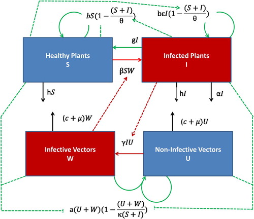
Figure 1. Compartmental diagram of the abundance-replanting model (2.3(2.1b) $\begin{array}{rl}\frac{\mathrm{d}I}{\mathrm{d}t}& =b\frac{ϵI}{S+ϵI}I\left(1-\frac{N}{\theta }\right)+\beta SW-(\alpha +h+g)I,\end{array}$(2.1b) ). The plant and vector susceptible compartments (Healthy Plants, Non-Infective Vectors) are coloured blue, while their infected compartments (Infected Plants, Infective Vectors) are coloured red. The solid lines indicate the compartment into which a new infection or transfer occurs, while the dotted lines indicate the compartments which are implicitly involved in a given new infection or transfer.

A more direct comparison of these two models can be seen in the logistic-type assumption for replanting. In each model, the replanting rate has the form $\mathrm{d}S/\mathrm{d}t=b_{S}S(1-N/\theta )$ and $\mathrm{d}I/\mathrm{d}t=b_{I}I(1-N/\theta )$, where the rates $b_S$ and $b_I$ for frequency-replanting are $b_S=\frac{bS}{S+ϵI},\mathrm{a}\mathrm{n}\mathrm{d}{b}_I=\frac{bϵI}{S+ϵI},$ and for abundance replanting they are $b_S=b,\mathrm{a}\mathrm{n}\mathrm{d}{b}_I=bϵ.$ It is clear from the expressions for $b_S$ and $b_I$ that for the same values of b, the replacement rate is slower for frequency-replanting than for abundance-replanting. In particular, as ε increases, the replacement rate is further reduced for the frequency-replanting model. If farmers can easily distinguish healthy plants from infected plants and there are sufficient number of healthy plants, then $ϵ=0$. In this case, the two models are in agreement.

For reference purposes, the variables in the models are defined in Table 1 and the parameters in Table 2. In all of the simulations, the parameter values in both models are strictly positive with the exception that α and c may be zero. Also, the initial conditions are positive. Parameter values for the models are taken from Holt et al. [14] and are summarized in Table 2. The two control parameters are the roguing rate, α, and the vector mortality due to insecticide use, c.

Table 1. Abundance (i.e. density) is measured in numbers per unit area.

Variable	Description
Host
N	Total abundance of host species (N:=S+I)
S	Abundance of healthy plant species
I	Abundance of infected plant species
Vector
V	Total abundance of vectors (V :=U+W)
U	Abundance of non-infective vectors
W	Abundance of infective vectors

Table 2. Parameters and their baseline values as in [14].

Parameter	Description	Range	Baseline Value
Host
b	maximum replanting rate (per day)	$[0.025,0.1]$	0.05
h	harvesting rate (per day)	$[0.002,0.004]$	0.003
r	rate of increase of healthy plant host (r:=b−h)	$[0.023,0.096]$	0.047
α	roguing rate (per day)	$[0,0.033]$	0.003
ε	selection of diseased cuttings for propagation	$[0,1.0]$	0.1
g	recovery rate from infection (per day)	[0.002, 0.004]	0.003
θ	maximum plant population pressure (per m^2)	$[0.01,1.0]$	0.5
K	maximum Host abundance (per m^2) ($K:=r\theta /b$)	$[0.01,1.0]$	0.47
Vector
a	maximum vector birth rate (per day)	$[0.1,0.3]$	0.2
μ	natural vector mortality (per day)	$[0.06,0.18]$	0.06
c	insecticide vector mortality (per day)	$[0,0.18]$	0.06
κ	maximum vector density per host plant	$[0,2500]$	500
$K_v$	maximum vector density (per m${}^2$) ($K_v:=q\kappa K/a$)	$[0,350]$	94
Pathogen
β	vector to host inoculation rate (per vector per day)	$[0.002,0.032]$.	0.008
γ	host to vector acquisition rate (per plant per day)	$[0.002,0.032]$	0.008

Notes: For the roguing rate (α) and insecticide vector mortality (c), the baseline values represent the values used in the sensitivity analysis. For the case of optimal control, where α and c are the control variables, the system is usually started at either equilibrium or non-equilibrium values in the absence of roguing and vector control, i.e. $\alpha =c=0$.

The total plant density for the frequency-replanting model (2.1(2.1b) $\begin{array}{rl}\frac{\mathrm{d}I}{\mathrm{d}t}& =b\frac{ϵI}{S+ϵI}I\left(1-\frac{N}{\theta }\right)+\beta SW-(\alpha +h+g)I,\end{array}$(2.1b) ) and the abundance-replanting model (2.3(2.1b) $\begin{array}{rl}\frac{\mathrm{d}I}{\mathrm{d}t}& =b\frac{ϵI}{S+ϵI}I\left(1-\frac{N}{\theta }\right)+\beta SW-(\alpha +h+g)I,\end{array}$(2.1b) ), respectively, are (2.4a) $\begin{array}{rl}\frac{\mathrm{d}N}{\mathrm{d}t}& =b\frac{S^2+ϵI^2}{S+ϵI}\left(1-\frac{N}{\theta }\right)-hN-\alpha I,\left(\mathtt{F}\mathtt{r}\mathtt{e}\mathtt{q}\mathtt{u}\mathtt{e}\mathtt{n}\mathtt{c}\mathtt{y}\mathtt{-}\mathtt{r}\mathtt{e}\mathtt{p}\mathtt{l}\mathtt{a}\mathtt{n}\mathtt{t}\mathtt{i}\mathtt{n}\mathtt{g}\mathtt{\right)}\mathtt{,}\end{array}$(2.4a) (2.4b) $\begin{array}{rl}\frac{\mathrm{d}N}{\mathrm{d}t}& =b(S+ϵI)\left(1-\frac{N}{\theta }\right)-hN-\alpha I,\left(\mathtt{A}\mathtt{b}\mathtt{u}\mathtt{n}\mathtt{d}\mathtt{a}\mathtt{n}\mathtt{c}\mathtt{e}\mathtt{-}\mathtt{r}\mathtt{e}\mathtt{p}\mathtt{l}\mathtt{a}\mathtt{n}\mathtt{t}\mathtt{i}\mathtt{n}\mathtt{g}\mathtt{\right)}\mathtt{.}\end{array}$(2.4b) The total host plant density is bounded by logistic growth with intrinsic growth rate r=b−h>0 and carrying capacity $K=\left(r\theta \right)/b$ (assuming $N\left(t\right)>0$), $\frac{\mathrm{d}N}{\mathrm{d}t}\le rN\left(1-\frac{N}{K}\right).$ The total vector density follows logistic growth provided the per capita rate $q=a-(\mu +c)>0$: $\frac{\mathrm{d}V}{\mathrm{d}t}=aV\left(1-\frac{V}{\kappa N}\right)-(\mu +c)V=qV\left(1-\frac{V}{pN}\right).$ For q>0, the vector carrying capacity is $K_v=pK<\kappa K$, where $p=\left(q\kappa \right)/a$, with κ the maximum vector density per host plant. We assume that initial conditions for the total plant and vector populations are bounded by their respective carrying capacities: (2.5) $0<V\left(0\right)<\kappa N\left(0\right)<\kappa K.$(2.5) In the absence of disease, I=0 and W=0, the two models are the same. The two models differ when plants are infected. As an example, suppose the selection parameter (frequency or rate) is $ϵ=1$, so that all plants, regardless of infection status, are selected for replanting and there is no roguing of infected plants, $\alpha =0$. The total plant density for the abundance-replanting model (2.3(2.1b) $\begin{array}{rl}\frac{\mathrm{d}I}{\mathrm{d}t}& =b\frac{ϵI}{S+ϵI}I\left(1-\frac{N}{\theta }\right)+\beta SW-(\alpha +h+g)I,\end{array}$(2.1b) ) follows logistic growth: (2.6) $\frac{\mathrm{d}N}{\mathrm{d}t}=rN\left(1-\frac{N}{K}\right).$(2.6) But in the frequency-replanting model (2.1(2.1b) $\begin{array}{rl}\frac{\mathrm{d}I}{\mathrm{d}t}& =b\frac{ϵI}{S+ϵI}I\left(1-\frac{N}{\theta }\right)+\beta SW-(\alpha +h+g)I,\end{array}$(2.1b) ), the total plant density grows slower than logistic: (2.7) $\frac{\mathrm{d}N}{\mathrm{d}t}=r\frac{S^2+I^2}{S+I}\left(1-\frac{N}{\theta }\right)-hN<rN\left(1-\frac{N}{K}\right).$(2.7) Some other differences in the two models are discussed in the next section.

3. Mathematical analysis

It follows from the differential equations for the total host population N and the initial conditions (2.5(2.5) $0<V\left(0\right)<\kappa N\left(0\right)<\kappa K.$(2.5) ) that if solutions for the plant and vector population models in (2.1(2.1b) $\begin{array}{rl}\frac{\mathrm{d}I}{\mathrm{d}t}& =b\frac{ϵI}{S+ϵI}I\left(1-\frac{N}{\theta }\right)+\beta SW-(\alpha +h+g)I,\end{array}$(2.1b) ) and (2.3(2.1b) $\begin{array}{rl}\frac{\mathrm{d}I}{\mathrm{d}t}& =b\frac{ϵI}{S+ϵI}I\left(1-\frac{N}{\theta }\right)+\beta SW-(\alpha +h+g)I,\end{array}$(2.1b) ) are nonnegative, then they are bounded above by their respective carrying capacities: $0<N\left(t\right)\le K$ and $0<V\left(t\right)\le K_v$ for $t\in [0,\mathrm{\infty })$. In addition, the vector density is bounded above by the density of the host population, (3.1) $0\le V\left(t\right)\le \kappa N\left(t\right)\le \kappa K,t\in [0,\mathrm{\infty }).$(3.1) In particular, it can be shown that the following region is invariant, $D=\left\{(S,I,U,W)\in {\mathbb{R}}_{+}^4|0\le S+I\le \kappa (U+W)\le \kappa K\right\},$ provided $h+\alpha \le \mu +c$ (Appendix 1). These conditions are satisfied for the baseline parameter values in Table 2 and for the range of the control parameters used in the numerical computations.

The disease-free equilibrium (DFE) for models (2.1(2.1b) $\begin{array}{rl}\frac{\mathrm{d}I}{\mathrm{d}t}& =b\frac{ϵI}{S+ϵI}I\left(1-\frac{N}{\theta }\right)+\beta SW-(\alpha +h+g)I,\end{array}$(2.1b) ) and (2.3(2.1b) $\begin{array}{rl}\frac{\mathrm{d}I}{\mathrm{d}t}& =b\frac{ϵI}{S+ϵI}I\left(1-\frac{N}{\theta }\right)+\beta SW-(\alpha +h+g)I,\end{array}$(2.1b) ) is $(S,I,U,W)=(K,0,K_v,0)$. The basic reproduction number near the DFE can be defined using the next generation matrix [33]. For frequency-replanting, the next generation matrix is (3.2) $M_F=\left[\begin{array}{cc}0& \frac{\beta K}{\mu +c}\\ \frac{\gamma K_v}{h+\alpha +g}& 0\end{array}\right],$(3.2) and for abundance-replanting, it is (3.3) $M_A=\left[\begin{array}{cc}\frac{hϵ}{h+\alpha +g}& \frac{\beta K}{\mu +c}\\ \frac{\gamma K_v}{h+\alpha +g}& 0\end{array}\right].$(3.3) Mathematically, the basic reproduction number is the eigenvalue of the next generation matrix with maximum modulus. Biologically, the basic reproduction number gives the number of secondary infections from one infected host or one infective vector, i.e. the number of infected plant hosts (infective vectors) generated from one infected host (infective vector). For frequency-replanting, the basic reproduction number is ${\mathcal{R}}_{0,F}=\sqrt{\frac{\beta \gamma K{K}_v}{(\mu +c)(h+\alpha +g)}},$ but for abundance-replanting it is (3.4) ${\mathcal{R}}_{0,A}=\frac{hϵ}{2(h+\alpha +g)}+\frac{1}{2}\sqrt{{\left(\frac{hϵ}{h+\alpha +g}\right)}^2+4\frac{\beta \gamma K{K}_v}{(\mu +c)(h+\alpha +g)}}.$(3.4) Notice for frequency-replanting that the basic reproduction does not depend on ε. The square root in ${\mathcal{R}}_{0,F}$ is due to the fact that it is the geometric mean for two generations: infection from the plant to the vector and then from the vector back to the plant (or vice versa). (When referring to both models, we will use the notation ${\mathcal{R}}_0$ for the basic reproduction number.) The DFE is locally asymptotically stable if ${\mathcal{R}}_0<1$ and unstable if ${\mathcal{R}}_0>1$ [33]. (Global stability of the DFE is verified in the special case of $ϵ=0$, Theorem A.2.)

Alternate but equivalent thresholds are the type reproduction numbers whose magnitude give an indication of the effort to eradicate the infection in the host plant, ${\mathcal{T}}_h$, or in the vector, ${\mathcal{T}}_v$ when the level of infection is low (near the DFE) [12,26]. For frequency-replanting, there are no differences in these thresholds, ${\mathcal{T}}_{h,F}={\mathcal{T}}_{v,F}=\frac{\beta \gamma K{K}_v}{(\mu +c)(h+\alpha +g)}.$ However, for abundance-replanting, the type reproduction number for host plants is (3.5) ${\mathcal{T}}_{h,A}=\frac{hϵ}{h+\alpha +g}+\frac{\beta \gamma K{K}_v}{(\mu +c)(h+\alpha +g)},$(3.5) and the type reproduction number for vectors is (3.6) $\begin{array}{rl}{\mathcal{T}}_{v,A}& =\frac{\beta \gamma K{K}_v}{(\mu +c)(h+\alpha +g)}{\left(1-\frac{hϵ}{h+\alpha +g}\right)}^{-1}\\ & =\frac{\beta \gamma K{K}_v}{(\mu +c)(h+\alpha +g)}\left(1+\frac{hϵ}{h+\alpha +g}+{\left[\frac{hϵ}{h+\alpha +g}\right]}^2+\cdots \right).\end{array}$(3.6) In the formula for ${\mathcal{T}}_{h,A}$, the two expressions represent the two sources of infection for the plant, either directly from replanting infected cuttings (vertical transmission) or indirectly from infective vectors. The terms in the expression for ${\mathcal{T}}_{v,A}$ represent vector infection indirectly from infected plants or indirectly from infected plants harvested in the first generation and replanted or from infected plants harvested in the second generation and replanted and so on.

It is interesting to note that the basic and the type reproduction numbers are larger in abundance-replanting than in frequency-replanting, meaning greater likelihood of disease outbreaks with abundance-replanting than frequency-replanting. In both replanting models (2.1(2.1b) $\begin{array}{rl}\frac{\mathrm{d}I}{\mathrm{d}t}& =b\frac{ϵI}{S+ϵI}I\left(1-\frac{N}{\theta }\right)+\beta SW-(\alpha +h+g)I,\end{array}$(2.1b) ) and (2.3(2.1b) $\begin{array}{rl}\frac{\mathrm{d}I}{\mathrm{d}t}& =b\frac{ϵI}{S+ϵI}I\left(1-\frac{N}{\theta }\right)+\beta SW-(\alpha +h+g)I,\end{array}$(2.1b) ), if ${\mathcal{R}}_0<1$ (or ${\mathcal{T}}_h<1$ or ${\mathcal{T}}_v<1)$, then the DFE is locally asymptotically stable and if the inequality is reversed, the DFE is unstable.

For the type reproduction numbers, it can be shown that one of the following three conditions holds, $\mathcal{T}<{\mathcal{R}}_0<1$, $\mathcal{T}>{\mathcal{R}}_0>1$ or $\mathcal{T}={\mathcal{R}}_0=1$ [3,26]. In particular, in the abundance-replanting model, one of the following relations holds: (3.7) ${\mathcal{T}}_{v,A}<{\mathcal{T}}_{h,A}<{\mathcal{R}}_{0,A}<1,{\mathcal{T}}_{v,A}>{\mathcal{T}}_{h,A}>{\mathcal{R}}_{0,A}>1,\mathrm{o}\mathrm{r}{\mathcal{T}}_{v,A}={\mathcal{T}}_{h,A}={\mathcal{R}}_{0,A}=1.$(3.7) If the basic reproduction number is greater than one, in the abundance-replanting model, the inequalities indicate that more effort may be required to eradicate infective vectors than infected plant hosts. In the frequency-replanting model, similar relations hold, as in (3.7(3.7) ${\mathcal{T}}_{v,A}<{\mathcal{T}}_{h,A}<{\mathcal{R}}_{0,A}<1,{\mathcal{T}}_{v,A}>{\mathcal{T}}_{h,A}>{\mathcal{R}}_{0,A}>1,\mathrm{o}\mathrm{r}{\mathcal{T}}_{v,A}={\mathcal{T}}_{h,A}={\mathcal{R}}_{0,A}=1.$(3.7) ), with the exception that ${\mathcal{T}}_{v,F}={\mathcal{T}}_{h,F}$ in all three cases. However, these expressions depend on the system state being near the DFE and in addition, they do not account for the costs associated with individual control measures, such as roguing or insecticide use, important in choosing environmentally and economically sound methods.

3.1. Endemic equilibria

Analytical formulas for the endemic equilibria (EE) cannot be computed explicitly for models (2.1(2.1b) $\begin{array}{rl}\frac{\mathrm{d}I}{\mathrm{d}t}& =b\frac{ϵI}{S+ϵI}I\left(1-\frac{N}{\theta }\right)+\beta SW-(\alpha +h+g)I,\end{array}$(2.1b) ) and (2.3(2.1b) $\begin{array}{rl}\frac{\mathrm{d}I}{\mathrm{d}t}& =b\frac{ϵI}{S+ϵI}I\left(1-\frac{N}{\theta }\right)+\beta SW-(\alpha +h+g)I,\end{array}$(2.1b) ), except in special cases as noted below. For the range of parameter values given in Table 2, the EE can be computed numerically.

Denote the EE as ($S^{\ast },I^{\ast },U^{\ast },W^{\ast })$. The endemic values for the vector can be computed from the differential equations $\mathrm{d}(U+W)/\mathrm{d}t=0$ and $\mathrm{d}W/\mathrm{d}t=0$ and can be expressed in terms of $S^{\ast }$ and $I^{\ast }$ as follows: (3.8a) $\begin{array}{rl}{U}^{\ast }& =\frac{\kappa (S^{\ast }+I^{\ast })q(\mu +c)}{a(\gamma I^{\ast }+\mu +c)},\end{array}$(3.8a) (3.8b) $\begin{array}{rl}{W}^{\ast }& =\frac{\kappa (S^{\ast }+I^{\ast })q\gamma I^{\ast }}{a(\gamma I^{\ast }+\mu +c)},\end{array}$(3.8b) where $q=a-(\mu +c)>0$. The EE values for $S^{\ast }$ and $I^{\ast }$ are the positive solutions of two nonlinear equations, computed from the differential equations for $d(S+I)/\mathrm{d}t=0$ and $\mathrm{d}I/\mathrm{d}t=0$. For the frequency-type model (2.1(2.1b) $\begin{array}{rl}\frac{\mathrm{d}I}{\mathrm{d}t}& =b\frac{ϵI}{S+ϵI}I\left(1-\frac{N}{\theta }\right)+\beta SW-(\alpha +h+g)I,\end{array}$(2.1b) ), the two nonlinear equations are (3.9a) $\begin{array}{rl}{F}_1(S,I)& =b\frac{S^2+ϵI^2}{S+ϵI}\left(1-\frac{N}{\theta }\right)-hN-\alpha I=0,\end{array}$(3.9a) (3.9b) $\begin{array}{rl}{F}_2(S,I)& =\frac{bϵI}{S+ϵI}\left(1-\frac{N}{\theta }\right)+\frac{\beta \kappa q\gamma SN}{a(\gamma I+\mu +c)}-(\alpha +h+g)=0,\end{array}$(3.9b) where N=S+I. For the abundance-type model (2.3(2.1b) $\begin{array}{rl}\frac{\mathrm{d}I}{\mathrm{d}t}& =b\frac{ϵI}{S+ϵI}I\left(1-\frac{N}{\theta }\right)+\beta SW-(\alpha +h+g)I,\end{array}$(2.1b) ), they are (3.10a) $\begin{array}{rl}{G}_1(S,I)& =b(S+ϵI)\left(1-\frac{N}{\theta }\right)-hN-\alpha I=0,\end{array}$(3.10a) (3.10b) $\begin{array}{rl}{G}_2(S,I)& =bϵ\left(1-\frac{N}{\theta }\right)+\frac{\beta \kappa q\gamma SN}{a(\gamma I+\mu +c)}-(\alpha +h+g)=0.\end{array}$(3.10b) The EE values for ($S^{\ast },I^{\ast }$) lie in the S-I plane, in the interior of the triangular region bounded by the lines S=0, I=0, and S+I=K (Equation (3.1(3.1) $0\le V\left(t\right)\le \kappa N\left(t\right)\le \kappa K,t\in [0,\mathrm{\infty }).$(3.1) ) and Theorem A.1). For the baseline values in Table 2 and the range of values for α and c, the solutions to models (2.1(2.1b) $\begin{array}{rl}\frac{\mathrm{d}I}{\mathrm{d}t}& =b\frac{ϵI}{S+ϵI}I\left(1-\frac{N}{\theta }\right)+\beta SW-(\alpha +h+g)I,\end{array}$(2.1b) ) and (2.3(2.1b) $\begin{array}{rl}\frac{\mathrm{d}I}{\mathrm{d}t}& =b\frac{ϵI}{S+ϵI}I\left(1-\frac{N}{\theta }\right)+\beta SW-(\alpha +h+g)I,\end{array}$(2.1b) ) are nonnegative (Theorem A.1).

We tested the existence and local stability of the EE for both models for the range of parameter values given for α, c, and ε and for the other baseline parameter values given in Table 2 that were considered in the sensitivity analysis and in the optimal control problems. The existence of EE for each model occur when the basic reproduction numbers, ${\mathcal{R}}_{0,F}>1$ or ${\mathcal{R}}_{0,A}>1$. There exists at most one locally stable EE for model (2.1(2.1b) $\begin{array}{rl}\frac{\mathrm{d}I}{\mathrm{d}t}& =b\frac{ϵI}{S+ϵI}I\left(1-\frac{N}{\theta }\right)+\beta SW-(\alpha +h+g)I,\end{array}$(2.1b) ). But for model (2.3(2.1b) $\begin{array}{rl}\frac{\mathrm{d}I}{\mathrm{d}t}& =b\frac{ϵI}{S+ϵI}I\left(1-\frac{N}{\theta }\right)+\beta SW-(\alpha +h+g)I,\end{array}$(2.1b) ), there exist parameter values for ε close to one, where two stable EE exist. In the case of bistability, the results depend on the initial data. For $ϵ\le 0.5$ and the range of parameter values considered, both models have at most one locally stable EE. In Appendix 2, graphs of the curves $F_i=0$ and $G_i=0$ for i=1,2, given by Equations (3.9a(3.9a) $\begin{array}{rl}{F}_1(S,I)& =b\frac{S^2+ϵI^2}{S+ϵI}\left(1-\frac{N}{\theta }\right)-hN-\alpha I=0,\end{array}$(3.9a) )–(3.9b(3.9b) $\begin{array}{rl}{F}_2(S,I)& =\frac{bϵI}{S+ϵI}\left(1-\frac{N}{\theta }\right)+\frac{\beta \kappa q\gamma SN}{a(\gamma I+\mu +c)}-(\alpha +h+g)=0,\end{array}$(3.9b) ) and (3.10a(3.10a) $\begin{array}{rl}{G}_1(S,I)& =b(S+ϵI)\left(1-\frac{N}{\theta }\right)-hN-\alpha I=0,\end{array}$(3.10a) )–(3.10b(3.10b) $\begin{array}{rl}{G}_2(S,I)& =bϵ\left(1-\frac{N}{\theta }\right)+\frac{\beta \kappa q\gamma SN}{a(\gamma I+\mu +c)}-(\alpha +h+g)=0.\end{array}$(3.10b) ), respectively, illustrate the unique locally stable EE for both models and a case of bistability for model (2.1(2.1b) $\begin{array}{rl}\frac{\mathrm{d}I}{\mathrm{d}t}& =b\frac{ϵI}{S+ϵI}I\left(1-\frac{N}{\theta }\right)+\beta SW-(\alpha +h+g)I,\end{array}$(2.1b) ) when $ϵ=1$.

The EE for the case $ϵ=0$ and $g=0$ for model (2.1(2.1b) $\begin{array}{rl}\frac{\mathrm{d}I}{\mathrm{d}t}& =b\frac{ϵI}{S+ϵI}I\left(1-\frac{N}{\theta }\right)+\beta SW-(\alpha +h+g)I,\end{array}$(2.1b) ) was computed by Holt et al. [14]. In this special case, all replanting is from virus-free cuttings and there is no reversion of infected plants. For $ϵ=0$, the two models are in agreement, so the EE values are the same for both models (2.1(2.1b) $\begin{array}{rl}\frac{\mathrm{d}I}{\mathrm{d}t}& =b\frac{ϵI}{S+ϵI}I\left(1-\frac{N}{\theta }\right)+\beta SW-(\alpha +h+g)I,\end{array}$(2.1b) ) and (2.3(2.1b) $\begin{array}{rl}\frac{\mathrm{d}I}{\mathrm{d}t}& =b\frac{ϵI}{S+ϵI}I\left(1-\frac{N}{\theta }\right)+\beta SW-(\alpha +h+g)I,\end{array}$(2.1b) ). Define the parameters η and δ as $\begin{array}{rl}\eta & =\frac{\beta K_v}{h+\alpha },\\ \delta & =\frac{h+\alpha }{r}+1.\end{array}$ Then the value of $S^{\ast }$ is the positive solution of the following quadratic equation which depends on ${\mathcal{R}}_0$: (3.11) $S^2-K\left(\frac{1+\eta /{\mathcal{R}}_0^2}{1+\eta \delta }\right)S-K^2\left(\frac{\eta (\delta -1)}{{\mathcal{R}}_0^2(1+\eta \delta )}\right)=0.$(3.11) There is only one positive root of this quadratic equation since the coefficient of S and the constant term are negative. The other EE values are computed in terms of $S^{\ast }$ as follows: (3.12a) $\begin{array}{rl}{I}^{\ast }& =\frac{r{S}^{\ast }(K-S^{\ast })}{(h+\alpha )K+r{S}^{\ast }},\end{array}$(3.12a) (3.12b) $\begin{array}{rl}{U}^{\ast }& =\frac{(h+\alpha )c}{\beta \gamma S^{\ast }},\end{array}$(3.12b) (3.12c) $\begin{array}{rl}{W}^{\ast }& =\frac{r(h+\alpha )(K-S^{\ast })}{\beta \left[\right(h+\alpha )K+r{S}^{\ast }]}.\end{array}$(3.12c) It also follows from the preceding definitions for the EE that the value of $N^{\ast }=S^{\ast }+I^{\ast }$ satisfies $0<N^{\ast }<K$ iff ${\mathcal{R}}_0>1$. Therefore, in the special case $ϵ=0=g$, the EE exists iff ${\mathcal{R}}_0>1$.

In [1,34], a simplified version of our base model was analyzed with $ϵ=0$ and g=0 and applied to the plant host J. curcas. The authors derive conditions for local stability of the EE and existence of a Hopf bifurcation as a function of the transmission parameter from infected vector to host plant. They show the existence of stable periodic solutions, as the bifurcation parameter is varied.

4. Numerical sensitivity analysis

In the remaining sections, we apply the two replanting models to a case study of ACMV. We check the sensitivity of the equilibrium values to variation in the two control parameters α and c. Parameters that are not varied are fixed at their baseline values given in Table 2. As can be seen in the Figures 2 and 3, as the death rate of vectors $c+\mu$ or roguing α increase, the infected plant density decreases. When selection preference for infected plants is low ($ϵ=0.1$), infected plant densities are smaller than for high selection preference for infected plants ($ϵ=1.0$). In addition, for low selection of infected plants $(ϵ=0.1)$, the infected plant density is generally greater in frequency-replanting than in abundance-replanting but this trend is slightly reversed for high selection parameter values ($ϵ=1.0$). Also comparing equilibrium densities for variation in $c+\mu$ to α, for the baseline value of α and a range of values for $c+\mu \in [0.06,0.18]$ equilibrium densities of infected plants are greater than for the baseline value of $c+\mu$ and a range of values for $\alpha \in [0,0.033]$. Lastly, there are sharp transitions between endemic levels of infection in frequency-replanting than in abundance-replanting, indicating a greater degree of sensitivity to model parameters in frequency-replanting. This latter effect is due to bistability in this parameter region.

Figure 2. The impact on the abundance at equilibrium of healthy cassava plants (solid line) and infected cassava plants (dashed line) with respect to change in parameters, $c+\mu$ and α. In the top figures α and in the bottom figures c+μ are fixed at their baseline values given in Table 2. The plots in the first column are for the case $ϵ=0$, plots in the middle column are for the case of abundance-replanting with $ϵ=0.1$. The plots in the last column are for frequency-replanting with $ϵ=0.1$.

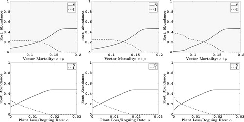
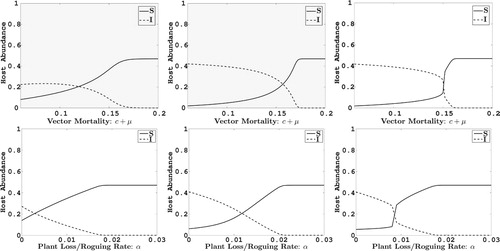
Figure 3. The impact on the abundance at equilibrium of healthy cassava plants (solid line) and infected cassava plants (dashed line) with respect to change in parameters $c+\mu$ and α. In the top figures α, and in the bottom figures c+μ are fixed at their baseline values given in Table 2. The plots in the first column are for the case $ϵ=0$, plots in the middle column are for the case of abundance-replanting with $ϵ=1.0$. The plots in the last column are for frequency-replanting with $ϵ=1.0$.

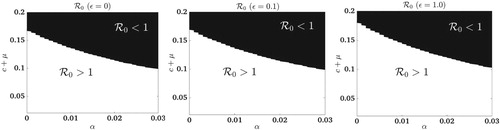
In Figure 4, regions in parameter space α and $c+\mu$ where the basic reproduction number is greater or less than one are graphed for three different values of ε. The three graphs correspond to ${\mathcal{R}}_{0,A}$ for abundance-replanting when $ϵ=0,$ 0.1 and 1.0. The graph on the left, $ϵ=0$, corresponds to frequency-replanting, ${\mathcal{R}}_{0,F}$ (which is not a function of ε). With roguing and insecticide applications, the value of the basic reproduction number decreases. For $0<ϵ\le 1$, the parameter region ${\mathcal{R}}_0>1$ is larger in the abundance-replanting model than in the frequency-replanting model.

Figure 4. For the abundance-replanting model, the region where the values of the basic reproduction number, ${\mathcal{R}}_{0,A}$, are less than or greater than one are graphed in parameter space as a function of roguing α and vector mortality $c+\mu$ with (Left Plot) $ϵ=0$, (Middle Plot) $ϵ=0.1$, (Right Plot) $ϵ=1.0$. In the frequency-replanting model, ${\mathcal{R}}_{0,F}$ is not dependent on ε. Thus, ${\mathcal{R}}_{0,F}$ is graphed in the left Plot (same for all values of ε).

5. Optimal control

According to Holt et al. [14], there are two main control approaches for African cassava mosaic disease (ACMD), either the use of phytosanitation methods or planting of resistant varieties. Phytosanitation consists of either using virus-free cuttings or removal of infected plants, i.e. roguing. Jeger et al. [15] state that vector control through insecticides is often ineffective and roguing may only contain the disease rather than eliminate it.

In this section, we apply optimal control to study the effect of the two control strategies, roguing and insecticide use. The two time-dependent control variables, $\alpha \left(t\right)\in [0,{\alpha }_{max}]$ and $c\left(t\right)\in [0,c_{max}]$, are described below.

1. Removal of infected plants from the field (roguing) with the objective of increasing the death rate of infected plants. $\alpha \to \alpha \left(t\right).$

2. Insecticide application with the objective of increasing the death rate of non-infective and infective vectors. $c\to c\left(t\right).$

Other types of control relate to planting strategies. Selection of resistant cultivars or virus-free cuttings may reduce the inoculation rate, parameter β, or the acquisition rate, parameter γ, or the abundance of infected cuttings for replanting, parameter ε. We do not consider variation in β or γ, but the optimal control results are investigated for a range of ε values.

In the simplified vector-host model with $ϵ=0$ and g=0, considered by Venturino et al. [34], the optimal control is shown to reduce the effect of oscillation in the system. The insecticide control in their paper is quite different from the one considered here. Their control depends on a time-dependent parameter that reduces the transmission from the infected vector to the susceptible plant which occurs through the use of time-dependent insecticide applications.

We define an objective functional with the goal to maximize a combination of the healthy plants harvested at the final time and the discounted stream of revenue from harvesting tubers from cassava plants less the cost of implementing the two controls: roguing and insecticide applications. When plants are infected, tuber yield is reduced because of poor quality of tubers or reduction in number of tubers per plant. Since the quality of tubers in infected plants is lower than healthy (susceptible) plants, we use parameters $p_1$ and $p_2$ to reflect this feature with $p_1>p_2$ to represent greater quality of tubers associated with harvest of healthy plants versus infected plants. The costs directly from applying the controls are represented with parameters, $A_1$ and $A_3$, for roguing and insecticide application, respectively, while the quadratic costs of controls with parameters, $A_2$ and $A_4$, represent damages to the long term crop yield from the roguing and insecticides (which are retained in the soil). Since the negative impacts of insecticides is greater than roguing, we choose $A_2{\alpha }_{\mathrm{m}\mathrm{a}\mathrm{x}}^2\ll A_4{c}_{\mathrm{m}\mathrm{a}\mathrm{x}}^2$. The discount on the revenue less the costs is given by the $e^{-\delta t}$ term. Removal of plants or roguing is labor intensive and insecticide applications are costly. Therefore, roguing and insecticide applications must be limited to ensure that gains from harvesting plants exceeds the costs associated with roguing and insecticide applications. The parameter $A_5$ gives the value of the salvage term at the end time, which indicates the importance of preserving plants for the following growing season. Therefore, the objective functional that we want to maximize over the finite time period $[0,T]$ is $\begin{array}{rl}J(\alpha ,c)& =A_{5}S\left(T\right)+{\int }_0^T{e}^{-\delta t}\left[p_{1}hS\left(t\right)+p_{2}hI\left(t\right)-A_1\alpha \left(t\right)I\left(t\right)-A_2{\alpha }^2\left(t\right)\right.\\ & -\left.A_{3}c\left(t\right)\left(U\right(t)+W(t\left)\right)-A_4{c}^2\left(t\right)\right]\mathrm{d}t.\end{array}$ We apply optimal control to compute $\underset{\{\alpha ,c\}}{max}J(\alpha ,c)$ on the time interval $[0,T]$, where $\alpha \left(t\right)\in [0,{\alpha }_{max}]$ and $c\left(t\right)\in [0,c_{max}]$ (see, e.g. [20,22]).

5.1. The optimality system

We define the set of admissible (bounded) control functions, $\mathbf{U}$ as (5.1) $\mathbf{U}=\{\mathbf{u}=[\alpha ,c{]}^T\in \left(L^{\mathrm{\infty }}\right(0,T){)}^2;(\alpha \left(t\right),c\left(t\right))\in [0,{\alpha }_{max}]\times [0,c_{max}],\mathrm{\forall }t\in [0,T\left]\right\}$(5.1) Our goal is to characterize an optimal control ${\mathbf{u}}^{\ast }=[{\alpha }^{\ast },c^{\ast }{]}^T\in \mathbf{U}$ satisfying (5.2) $J\left({\mathbf{u}}^{\ast }\right)=\underset{\mathbf{u}\in \mathbf{U}}{max}J\left(\mathbf{u}\right).$(5.2) We use standard results from optimal control theory to solve the optimal control problem [20,25], for both the abundance and the frequency-replanting models. The existence of the optimal control follows from the structure of the state system and the uniform $L^{\mathrm{\infty }}$ bounds on the states and the controls [17]. To characterize the optimal controls, we use Pontryagin's Maximum Principle [20], which requires the use of adjoint functions to transform the optimization problem into a problem of determining the pointwise maximum of the corresponding Hamiltonian. We derive necessary conditions on the optimal control as follows. Assume ${\mathbf{u}}^{\ast }$ is an optimal control and S,I,U,W are state responses to ${\mathbf{u}}^{\ast }$. We analyse the abundance-replanting model first.

5.1.1. Abundance-Replanting model

In this case, the Hamiltonian is: (5.3) $\begin{array}{rl}{\mathcal{H}}_A& =e^{-\delta t}\left[p_{1}hS+p_{2}hI-A_1\alpha I-A_2{\alpha }^2-A_{3}c(U+W)-A_4{c}^2\right]\\ & +{\lambda }_{1,A}\left(bS\left(1-\frac{N}{\theta }\right)-\beta SW-hS+gI\right)\\ & +{\lambda }_{2,A}\left(bϵI\left(1-\frac{N}{\theta }\right)+\beta SW-(\alpha +h+g)I\right)\\ & +{\lambda }_{3,A}\left(aV\left(1-\frac{V}{\kappa N}\right)-\gamma IU-(\mu +c)U\right)\\ & +{\lambda }_{4,A}\left(\gamma IU-(\mu +c)W\right),\end{array}$(5.3) with ${\mathit{\lambda }}_A=[{\lambda }_{1,A},{\lambda }_{2,A},{\lambda }_{3,A},{\lambda }_{4,A}{]}^T$, the adjoint vector associated to the state solution $\mathbf{X}=[S,I,U,W{]}^T$, of the ODEs associated to the abundance-replanting model. The time evolution of the adjoint functions can be determined by Pontryagin's Maximum Principle. The optimality system of equations results from taking the appropriate partial derivatives of the Hamiltonian with respect to the associated state variable. The optimality system for the abundance-replanting model consists of the state and adjoint systems together with a characterization of the control variables, which we now determine.

Theorem 5.1

There exists an optimal control ${\mathbf{u}}_A^{\ast }$ and state solution of the abundance-replanting model, $X_A^{\ast }=[S_A^{\ast },I_A^{\ast },U_A^{\ast },W_A^{\ast }{]}^T,$ that maximizes $J\left(\mathbf{u}\right)$ over the set $\mathbf{U}$. The associated adjoint functions ${\mathit{\lambda }}_A\left(t\right)$ with transversality $($final time$)$ conditions (5.4a) $\begin{array}{rl}& {\lambda }_{1,A}\left(T\right)=A_5,\end{array}$(5.4a) (5.4b) $\begin{array}{rl}& {\lambda }_{2,A}\left(T\right)={\lambda }_{3,A}\left(T\right)={\lambda }_{4,A}\left(T\right)=0,\end{array}$(5.4b) satisfy the evolution system (5.5a) $\begin{array}{rl}\frac{\mathrm{d}{\lambda }_{1,A}}{\mathrm{d}t}& =-\left[e^{-\delta t}{p}_{1}h+{\lambda }_{1,A}\left(b\left(1-\frac{N}{\theta }\right)-\frac{bS}{\theta }-\beta W-h\right)+{\lambda }_{2,A}\left(-\frac{bϵI}{\theta }+\beta W\right)\right.\\ & \left.+{\lambda }_{3,A}\left(\frac{a{V}^2}{\kappa N^2}\right)\right],\end{array}$(5.5a) (5.5b) $\begin{array}{rl}\frac{\mathrm{d}{\lambda }_{2,A}}{\mathrm{d}t}& =-\left[e^{-\delta t}(p_{2}h-A_1{\alpha }^{\ast })+{\lambda }_{1,A}\left(-\frac{bS}{\theta }+g\right)+{\lambda }_{2,A}\left(bϵ\left(1-\frac{N}{\theta }\right)\right.\right.\\ & -\left.\frac{bϵI}{\theta }-({\alpha }^{\ast }+h+g)\right)\left.+{\lambda }_{3,A}\left(\frac{a{V}^2}{\kappa N^2}-\gamma U\right)+{\lambda }_{4,A}\gamma U\right],\end{array}$(5.5b) (5.5c) $\begin{array}{rl}\frac{\mathrm{d}{\lambda }_{3,A}}{\mathrm{d}t}& =-\left[e^{-\delta t}(-A_3{c}^{\ast })+{\lambda }_{3,A}\left(a\left(1-2\frac{V}{\kappa N}\right)-\gamma I-(\mu +c^{\ast })\right)+{\lambda }_{4,A}\gamma I\right],\end{array}$(5.5c) (5.5d) $\begin{array}{rl}\frac{\mathrm{d}{\lambda }_{4,A}}{\mathrm{d}t}& =-\left[e^{-\delta t}(-A_3{c}^{\ast })-{\lambda }_{1,A}\beta S+{\lambda }_{2,A}\beta S+{\lambda }_{3,A}a\left(1-2\frac{V}{\kappa N}\right)-{\lambda }_{4,A}(\mu +c^{\ast })\right].\end{array}$(5.5d) Finally, the optimal control ${\mathbf{u}}^{\ast }=[{\alpha }_A^{\ast },c_A^{\ast }]$ satisfies the characterization (5.6) $\begin{array}{rl}{\alpha }_A^{\ast }\left(t\right)& =\mathrm{m}\mathrm{i}\mathrm{n}\left\{\mathrm{m}\mathrm{a}\mathrm{x}\left\{0,-\frac{A_{1}I\left(t\right)+e^{\delta t}{\lambda }_{2,A}\left(t\right)I\left(t\right)}{2A_2}\right\},{\alpha }_{max}\right\},\end{array}$(5.6) (5.7) $\begin{array}{rl}{c}_A^{\ast }\left(t\right)& =\mathrm{m}\mathrm{i}\mathrm{n}\left\{\mathrm{m}\mathrm{a}\mathrm{x}\left\{0,-\frac{A_3\left(U\right(t)+W(t\left)\right)+e^{\delta t}\left({\lambda }_{3,A}\right(t\left)U\right(t)+{\lambda }_{4,A}(t\left)W\right(t\left)\right)}{2A_4}\right\},c_{max}\right\}.\end{array}$(5.7)

The proof is given in Appendix 3. Thus, the system which characterizes the optimal control, the optimality system is given by

1. The forward problem for the state variables S,I,U,W given in model (2.3(2.1b) $\begin{array}{rl}\frac{\mathrm{d}I}{\mathrm{d}t}& =b\frac{ϵI}{S+ϵI}I\left(1-\frac{N}{\theta }\right)+\beta SW-(\alpha +h+g)I,\end{array}$(2.1b) ) with $\alpha ={\alpha }_A^{\ast }$ given in (5.6(5.6) $\begin{array}{rl}{\alpha }_A^{\ast }\left(t\right)& =\mathrm{m}\mathrm{i}\mathrm{n}\left\{\mathrm{m}\mathrm{a}\mathrm{x}\left\{0,-\frac{A_{1}I\left(t\right)+e^{\delta t}{\lambda }_{2,A}\left(t\right)I\left(t\right)}{2A_2}\right\},{\alpha }_{max}\right\},\end{array}$(5.6) ) and $c=c_A^{\ast }$ as given in (5.7(5.7) $\begin{array}{rl}{c}_A^{\ast }\left(t\right)& =\mathrm{m}\mathrm{i}\mathrm{n}\left\{\mathrm{m}\mathrm{a}\mathrm{x}\left\{0,-\frac{A_3\left(U\right(t)+W(t\left)\right)+e^{\delta t}\left({\lambda }_{3,A}\right(t\left)U\right(t)+{\lambda }_{4,A}(t\left)W\right(t\left)\right)}{2A_4}\right\},c_{max}\right\}.\end{array}$(5.7) ), along with the initial conditions $S\left(0\right)=S_0,I\left(0\right)=I_0,U\left(0\right)=U_0$ and $W\left(0\right)=W_0$.

2. The backward problem for the adjoint variables ${\lambda }_{1,A},{\lambda }_{2,A},{\lambda }_{3,A},{\lambda }_{4,A}$ given in system (5.5(2.2) $b\left(1-\frac{N}{\theta }\right).$(2.2) ) with $\alpha ={\alpha }_A^{\ast }$ given in (5.6(5.6) $\begin{array}{rl}{\alpha }_A^{\ast }\left(t\right)& =\mathrm{m}\mathrm{i}\mathrm{n}\left\{\mathrm{m}\mathrm{a}\mathrm{x}\left\{0,-\frac{A_{1}I\left(t\right)+e^{\delta t}{\lambda }_{2,A}\left(t\right)I\left(t\right)}{2A_2}\right\},{\alpha }_{max}\right\},\end{array}$(5.6) ) and $c=c_A^{\ast }$ as given in (5.7(5.7) $\begin{array}{rl}{c}_A^{\ast }\left(t\right)& =\mathrm{m}\mathrm{i}\mathrm{n}\left\{\mathrm{m}\mathrm{a}\mathrm{x}\left\{0,-\frac{A_3\left(U\right(t)+W(t\left)\right)+e^{\delta t}\left({\lambda }_{3,A}\right(t\left)U\right(t)+{\lambda }_{4,A}(t\left)W\right(t\left)\right)}{2A_4}\right\},c_{max}\right\}.\end{array}$(5.7) ), along with the final conditions ${\lambda }_{1,A}\left(T\right)=A_5,{\lambda }_{2,A}\left(T\right)=0,{\lambda }_{3,A}\left(T\right)=0,{\lambda }_{4,A}\left(T\right)=0$.

5.1.2. Frequency-Replanting model

In this case, the Hamiltonian is: (5.8) $\begin{array}{rl}{\mathcal{H}}_F& =e^{-\delta t}\left[p_{1}hS+p_{2}hI-A_1\alpha I-A_2{\alpha }^2-A_{3}c(U+W)-A_4{c}^2\right]\\ & +{\lambda }_{1,F}\left(b\frac{S}{S+ϵI}S\left(1-\frac{N}{\theta }\right)-\beta SW-hS+gI\right)\\ & +{\lambda }_{2,F}\left(b\frac{ϵI}{S+ϵI}I\left(1-\frac{N}{\theta }\right)+\beta SW-(\alpha +h+g)I\right)\\ & +{\lambda }_{3,F}\left(aV\left(1-\frac{V}{\kappa N}\right)-\gamma IU-(\mu +c)U\right)\\ & +{\lambda }_{4,F}\left(\gamma IU-(\mu +c)W\right),\end{array}$(5.8) where the adjoint ${\lambda }_F=[{\lambda }_{1,F},{\lambda }_{2,F},{\lambda }_{3,F},{\lambda }_{4,F}{]}^T$ satisfies a system similar to the one given for abundance-replanting. In addition, there exists an optimal control for frequency-replanting following an argument similar to that given in Theorem 5.1 (Appendix 4).

6. Numerical computation of the optimality system

We solve the optimality system associated with both the frequency and abundance-replanting models numerically to obtain the optimal controls. A forward-backward sweep iterative method (with a relaxation parameter $\hat{\theta }$) is used to solve the optimal control problem [20]. The initial guess of the control is its upper bound. Inside the iterative loop ODE15s is used to solve the state systems, given the stiff nature of these systems, and ODE45 is used to solve the adjoint systems.

The value T=100 (days) was chosen to represent a single growing season. The parameters of the objective functional (costs and prices) are highly dependent on the circumstances of individual scenarios. Thus, we explore some reasonable values by first determining a baseline case and then investigating the qualitative behavior of perturbations to those parameters.

Baseline case:

The range of values for $A_i$, $i=1,\dots ,5$ and $p_j$, j=1,2 was chosen to identify a baseline case which is sensitive to changes in each parameter, thus, representing a balance of mechanisms. In particular, $A_5$ and $A_4$ were set equal to one, and subsequently $A_3$ was chosen to provide balance in the c only control problem. The parameter $A_2$ was fixed in order to enforce $A_2{\alpha }_{max}^2\ll 2A_4{c}_{max}^2$, and subsequently $A_1$ was chosen to provide balance in the α only control problem. The price $p_2$ was chosen arbitrarily, and $p_1$ was chosen to be much greater. Finally, we set $\delta =0.02\mathrm{\%}$ annual rate. (6.1a) $\begin{array}{rl}\text{Costs: }& A_1=0.1,A_2=2,A_3=0.0005,A_4=1,\end{array}$(6.1a) (6.1b) $\begin{array}{rl}\text{Prices: }& A_5=1,p_1=100,p_2=1.\end{array}$(6.1b)

6.1. Baseline case results

The figures below are the result of numerical computations of the optimal controls using system parameters given in Table 2 for both models, including upper and lower bounds for the controls $\alpha \left(t\right)$ and $c\left(t\right)$, and $ϵ=0.1$. In each case, the initial conditions of the system are the respective equilibria for the particular uncontrolled replanting model: $\begin{array}{rl}{S}_0& =0.0182,I_0=0.438,U_0=150.97,\\ W_0& =8.82\mathtt{F}\mathtt{r}\mathtt{e}\mathtt{q}\mathtt{u}\mathtt{e}\mathtt{n}\mathtt{c}\mathtt{y}\mathtt{-}\mathtt{R}\mathtt{e}\mathtt{p}\mathtt{l}\mathtt{a}\mathtt{n}\mathtt{t}\mathtt{i}\mathtt{n}\mathtt{g}\mathtt{M}\mathtt{o}\mathtt{d}\mathtt{e}\mathtt{l}\\ S_0& =0.0360,I_0=0.309,U_0=116.03,\\ W_0& =4.78\mathtt{A}\mathtt{b}\mathtt{u}\mathtt{n}\mathtt{d}\mathtt{a}\mathtt{n}\mathtt{c}\mathtt{e}\mathtt{-}\mathtt{R}\mathtt{e}\mathtt{p}\mathtt{l}\mathtt{a}\mathtt{n}\mathtt{t}\mathtt{i}\mathtt{n}\mathtt{g}\mathtt{M}\mathtt{o}\mathtt{d}\mathtt{e}\mathtt{l}\end{array}$ The values of the objective functional from various cases are given in Table 3 for the frequency and abundance-replanting models, including no controls (top row), only α, only c, and both controls α and c (bottom row). With these baseline case parameter choices, strategic (non-zero) use of both controls is optimal for each replanting model, however, using either optimal roguing or optimal insecticide is preferable over the uncontrolled case. Specifically, for the frequency model, single controls are marginally better in J than no control, and dual controls are approximately three times better. However, for the abundance model, single controls, in particular roguing, is significantly better than no control, and the objective functional is nearly four times greater. We also note that with these baseline case parameter values, there is no scenario for which sustained maximum control is optimal. Details of the optimal controls and the system responses for the frequency-replanting and abundance-replanting models are given in Figures 5 and 6, respectively.

Figure 5. Frequency, equilibrium initial conditions, $ϵ=0.1$: (Top row) Optimal control results for roguing (${\alpha }^{\ast }$) and vector control through insecticides ($c^{\ast }$) for frequency-replanting for the cases of no control, only roguing (α), only vector control through insecticides (c), and roguing and vector control (α and c). (Bottom two rows) Optimally controlled system response in the four cases considered for roguing (${\alpha }^{\ast }$) and vector control ($c^{\ast }$) for frequency-replanting. The cases of roguing (α), insecticide (c), and roguing and insecticide (α and c) combined are contrasted with the uncontrolled system response.

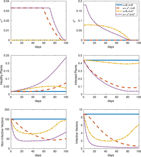
Figure 6. Abundance, equilibrium initial conditions, $ϵ=0.1$: Optimal control results for abundance-replanting for the cases of no control, only roguing (α), only vector control (c), and both roguing and vector control (α and c). Optimally controlled system response in the four cases considered for roguing (${\alpha }^{\ast }$) and vector control ($c^{\ast }$) for abundance-replanting. The cases of roguing (α only), insecticide (c only), and both roguing and insecticide (α and c) combined are contrasted with the uncontrolled system response.

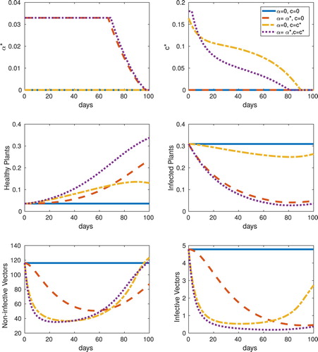
Table 3. Optimal control results for the baseline case.

${\alpha }_{max}$	$c_{max}$	$J\left(F\right)$	$J\left(A\right)$
0	0	0.693	1.205
0.033	0	0.820	2.934
0	0.18	0.793	2.028
0.033	0.18	2.070	4.339

Notes: We consider three types of control strategies, namely, roguing or insecticide use, or both roguing and insecticide use. For each case, we record values of the (optimal) objective functional: $J\left(F\right)$ for frequency-replanting, and $J\left(A\right)$ for abundance-replanting. For reference, the first row is the uncontrolled case. See Figures 5 and 6.

As expected, the roguing-only optimal controls decrease the infected plant hosts significantly more than do the insecticide-only optimal controls. On the other hand, the insecticide-only controls rapidly eliminate vectors initially, but they recover over the finite time horizon, whereas the roguing-only controls keep infective vector levels low up to the final time. With combined controls, both infected plant hosts and vectors are kept low, which results in significantly more susceptible hosts at the final time. This is especially true for the frequency- replanting model. Another difference between the two models for equilibrium initial conditions is that the optimal c for insecticide-only (optimal c) in the frequency-replanting model is less than half of its maximum constraint.

6.2. Selection parameter variations

We explore the effect of varying the selection parameter ε by computing the optimal controls for different values of ε for equilibrium initial conditions (see Table 4 and Figure 7).

Figure 7. Frequency (top) and abundance (bottom) with equilibrium initial conditions: Optimal controls for different values of the parameter ε. In the results for the abundance-replanting model, as ε increases the optimal control also increase. However, this is not the case in the results for the frequency-replanting model.

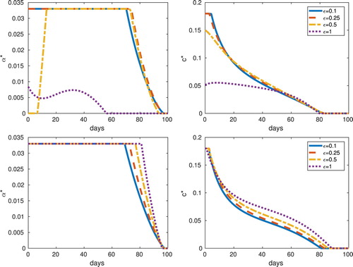
Table 4. Equilibrium solutions for various values of ε for frequency-replanting and abundance-replanting models.

	Frequency-replanting model				Abundance-replanting model
ε	$S_0$	$I_0$	$U_0$	$W_0$	$S_0$	$I_0$	$U_0$	$W_0$
0.1	0.018	0.438	150.966	8.823	0.036	0.309	116.032	4.784
0.25	0.018	0.446	153.304	9.123	0.025	0.374	132.897	6.631
0.5	0.018	0.449	154.049	9.220	0.020	0.423	146.646	8.263
1.0	0.018	0.450	154.416	9.268	0.018	0.452	155.152	9.348

For the abundance-replanting model there are slight differences between the case of $ϵ=1.0$ and the baseline case with $ϵ=0.1$. However, for the frequency-replanting model, the differences are more evident. When $ϵ=1.0$ in frequency-replanting, the optimal roguing levels are close to zero and the optimal vector control (insecticide) rates are much less than the case $ϵ=0.1$. However, by decreasing costs of the quadratic roguing term in the objective functional, we found that the optimal control results produced time profiles having greater roguing and insecticide control. Thus, the optimal control method using the frequency-replanting model seems to have a non-monotone dependence on costs and the selection frequency ε.

6.3. Non-equilibrium initial conditions

Finally, we explore the effect of varying the initial conditions away from the equilibrium values by computing the optimal controls for the case of the following (arbitrary) non-equilibrium values (6.2) $S_0=0.1,I_0=0.4,U_0=100,W_0=25.$(6.2) Details of the optimal control and a comparison of the results for equilibrium and non-equilibrium initial conditions are summarized in Figure 8 and Table 5. The non-equilibrium initial conditions have more infective vectors and more susceptible hosts than the equilibrium initial conditions. We do not see major differences in the abundance-replanting model results for the case of roguing and vector control by insecticides when starting at non-equilibrium initial conditions as compared to the results starting at equilibrium initial conditions. This remains true for different values of ε.

Figure 8. Frequency (top), abundance (bottom), non-equilibrium initial conditions: Optimal controls, ${\alpha }^{\ast }$ and $c^{\ast }$ for different values of ε.

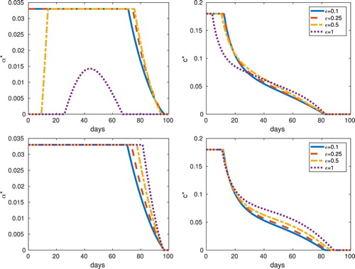
Table 5. Optimal control results for roguing and insecticide control using various values of the selection parameter ε.

	Basic reproduction number		Equilibrium		Non-equilibrium
ε	${\mathcal{R}}_{0,F}$	${\mathcal{R}}_{0,A}$	$J\left(F\right)$	$J\left(A\right)$	$J\left(F\right)$	$J\left(A\right)$
0.1	5.408	5.458	2.070	4.340	2.099	2.845
0.25	5.408	5.533	1.321	3.286	1.404	2.603
0.5	5.408	5.659	0.806	2.584	0.864	2.418
1.0	5.408	5.914	0.728	1.854	0.687	1.885

Notes: For each value of ε, we record the basic reproduction number and the (optimal) objective functional: $J\left(F\right)$ for frequency-replanting, and $J\left(A\right)$ for abundance type replanting. Equilibrium and non-equilibrium initial conditions are compared.

In the frequency-replanting model, we do see differences between results with equilibrium initial conditions and those with non-equilibrium initial conditions, when the value of ε is increased. In particular, when $ϵ=1$, the optimal roguing and insecticide controls have different time profiles but this may be expected since with $ϵ=1$, there exist a range of parameter values where there are multiple stable equilibria in model (2.1(2.1b) $\begin{array}{rl}\frac{\mathrm{d}I}{\mathrm{d}t}& =b\frac{ϵI}{S+ϵI}I\left(1-\frac{N}{\theta }\right)+\beta SW-(\alpha +h+g)I,\end{array}$(2.1b) ). Therefore, the time at which the control is applied is affected by the initial conditions. Thus, the optimal control strategies with the frequency-replanting model can be much different from those with the abundance-replanting model.

7. Conclusion

Mathematical models are increasingly being used in plant virus epidemiology to identify areas in which there is a greater potential use in both understanding disease dynamics and using this understanding to underpin disease control [16]. In this paper, we constructed a model that incorporates a new replanting strategy called abundance-type replanting. In this model, stem cuttings from both susceptible and infected plants can be used for replanting, with infected plants chosen based on some fixed selection parameter value that depends on plant abundance. We compare our model with a model for replanting by Holt et al. [14] and Jeger et al. [15] in which infected plants are used for replanting based on a fixed frequency of selection. This model was termed frequency-replanting in [15]. In both models, the parameter indicating the different type of selection mechanism for choosing infected plant cuttings is denoted by the same parameter ε.

We compare both the models using three different tools: (1) mathematical analysis based on threshold parameters; the basic and type reproduction numbers, (2) numerical sensitivity analysis of equilibria and (3) optimal control. In all three cases, we highlight the differences in the model results.

Our analytical results show that near the DFE, the parameter ε has no effect on the basic reproduction number ${\mathcal{R}}_{0,F}$ in the frequency-replanting model, but increasing ε in the abundance-replanting model increases the basic reproduction number ${\mathcal{R}}_{0,A}$. This implies that greater control is required to eradicate the disease at a low level of infection in the case of abundance-replanting as compared to frequency-replanting.

Optimal control strategies for the two replanting models result in different outcomes. The selection parameter, denoted ε in both models, has different interpretations: either as a frequency of selection of infected plants in frequency-replanting or as a rate of reduction of replanting of infected plants in abundance-replanting. Thus, a direct comparison of results of optimal control strategies should be made with caution. We used both equilibrium initial conditions as well as arbitrary, non-equilibrium, initial conditions to obtain the optimal control results. For control using roguing and insecticide use, we did see significant differences in the overall optimal roguing and insecticide controls that are produced by the optimal control strategy, especially near $ϵ=1$. The equilibria for the frequency-replanting model are sensitive to ε. Greater frequency of selection of infected plants may result in unanticipated outcomes when controls are applied. In conclusion, we observe that while farmers may not consciously choose between a frequency-replanting or abundance-replanting strategy, a well thought out plan for replanting is recommended. Our results suggest that different optimal control strategies are appropriate for the two distinct replanting practices.

Acknowledgments

This work was conducted as a part of the Multiscale Vectored Plant Viruses Investigative Workshop and a short-term visit by VAB and LJSA at the National Institute for Mathematical and Biological Synthesis.

Disclosure statement

No potential conflict of interest was reported by the authors.

Additional information

Funding

This work was assisted by a short-term visit and by an investigative workshop on Vectored Plant Viruses at the National Institute for Mathematical and Biological Synthesis, an Institute supported by the National Science Foundation (USA) through NSF Award #DBI-1300426, with additional support from The University of Tennessee, Knoxville.

Appendix 1. Nonnegative solutions and DFE

It is verified that solutions to models (2.1(2.1b) $\begin{array}{rl}\frac{\mathrm{d}I}{\mathrm{d}t}& =b\frac{ϵI}{S+ϵI}I\left(1-\frac{N}{\theta }\right)+\beta SW-(\alpha +h+g)I,\end{array}$(2.1b) ) and (2.3(2.1b) $\begin{array}{rl}\frac{\mathrm{d}I}{\mathrm{d}t}& =b\frac{ϵI}{S+ϵI}I\left(1-\frac{N}{\theta }\right)+\beta SW-(\alpha +h+g)I,\end{array}$(2.1b) ) are nonnegative. In addition, a sufficient condition for global stability of the DFE is given for model (2.3(2.1b) $\begin{array}{rl}\frac{\mathrm{d}I}{\mathrm{d}t}& =b\frac{ϵI}{S+ϵI}I\left(1-\frac{N}{\theta }\right)+\beta SW-(\alpha +h+g)I,\end{array}$(2.1b) ).

Theorem A.1

If $h+\alpha \le \mu +c,$ then solutions of the frequency-replanting model (2.1(2.1b) $\begin{array}{rl}\frac{\mathrm{d}I}{\mathrm{d}t}& =b\frac{ϵI}{S+ϵI}I\left(1-\frac{N}{\theta }\right)+\beta SW-(\alpha +h+g)I,\end{array}$(2.1b) ) and the abundance-replanting model (2.3(2.1b) $\begin{array}{rl}\frac{\mathrm{d}I}{\mathrm{d}t}& =b\frac{ϵI}{S+ϵI}I\left(1-\frac{N}{\theta }\right)+\beta SW-(\alpha +h+g)I,\end{array}$(2.1b) ) are contained in the region D.

Proof.

Checking the boundary of ${\mathbb{R}}_{+}^4$, it is straightforward to verify that the derivatives of $S,I,$ and W of both types of replanting models (2.1(2.1b) $\begin{array}{rl}\frac{\mathrm{d}I}{\mathrm{d}t}& =b\frac{ϵI}{S+ϵI}I\left(1-\frac{N}{\theta }\right)+\beta SW-(\alpha +h+g)I,\end{array}$(2.1b) ) and (2.3(2.1b) $\begin{array}{rl}\frac{\mathrm{d}I}{\mathrm{d}t}& =b\frac{ϵI}{S+ϵI}I\left(1-\frac{N}{\theta }\right)+\beta SW-(\alpha +h+g)I,\end{array}$(2.1b) ) are non-negative. For U=0, $\dot{U}\ge 0$ if $aW(1-W/\kappa N)\ge 0.$ From the differential equations for the total population size, it follows that $N\left(t\right)\le K$. Thus, to ensure solutions are non-negative, all we need to show is that $V\left(t\right)\le \kappa N\left(t\right)$ for t>0. This inequality will be shown to hold if $h+\alpha \le \mu +c$. Consider the triangular region in the V -N plane, where $(V,N)\in {\mathbb{R}}_{+}^2$ is bounded by N=K, V =0 and $V=\kappa N$. Assume initial values lie in the interior of D. Suppose $t_0>0$ is the first time such that $V\left(t_0\right)=\kappa N\left(t_0\right)$, i.e. for $t\in [0,t_0)$ $V\left(t\right)<\kappa N\left(t\right)$. Let $V\left(t_0\right)=V_0$, $S\left(t_0\right)=S_0$ and $I\left(t_0\right)=I_0$. Note that $\mathrm{d}V/\mathrm{d}t<0$ when $V_0=\kappa N_0>0$. Therefore, to ensure solutions to do not cross the boundary $V=\kappa N$ and leave the triangular region, we only need to consider the case where $\mathrm{d}N/\mathrm{d}t<0$ and show that $\mathrm{d}V/\mathrm{d}t-\kappa \mathrm{d}N/\mathrm{d}t<0$ at $t=t_0$. The expression $\mathrm{d}V/\mathrm{d}t-\kappa \mathrm{d}N/\mathrm{d}t$ can be written in terms of $S_0$, $I_0$ and $N_0$ as follows: (A1) $A=\kappa \left[\frac{bf(S_0,I_0)(N_0-\theta )}{\theta }+(h-\mu -c)N_0+\alpha I_0\right],$(A1) where $f(S_0,I_0)$ is either $S_0+ϵI_0$ or $(S_0^2+ϵI_0^2)/(S_0+ϵI_0)$ in both types of replanting models (2.1(2.1b) $\begin{array}{rl}\frac{\mathrm{d}I}{\mathrm{d}t}& =b\frac{ϵI}{S+ϵI}I\left(1-\frac{N}{\theta }\right)+\beta SW-(\alpha +h+g)I,\end{array}$(2.1b) ) or (2.3(2.1b) $\begin{array}{rl}\frac{\mathrm{d}I}{\mathrm{d}t}& =b\frac{ϵI}{S+ϵI}I\left(1-\frac{N}{\theta }\right)+\beta SW-(\alpha +h+g)I,\end{array}$(2.1b) ), respectively. Expressing the inequality $N_0\le K$ in terms of the original parameters leads to the inequality $N_0-\theta \le -\frac{h}{b}\theta .$ Therefore, the first term in the square brackets in (A1(A1) $A=\kappa \left[\frac{bf(S_0,I_0)(N_0-\theta )}{\theta }+(h-\mu -c)N_0+\alpha I_0\right],$(A1) ) is negative and $A\le \kappa \left(h+\alpha -(\mu +c)\right)I_0-(\mu +c)S_0.$ If $h+\alpha \le \mu +c$, the right side of the preceding expression is negative. Hence, $\mathrm{d}V/\mathrm{d}t-\kappa \mathrm{d}N/\mathrm{d}t\le 0$.

Theorem A.2

The DFE for the Abundance-Replanting model (2.3(2.1b) $\begin{array}{rl}\frac{\mathrm{d}I}{\mathrm{d}t}& =b\frac{ϵI}{S+ϵI}I\left(1-\frac{N}{\theta }\right)+\beta SW-(\alpha +h+g)I,\end{array}$(2.1b) ) is globally asymptotically stable if the following condition is satisfied ${\mathcal{R}}_{ϵ}:=\frac{bϵ}{h+\alpha +g}+\frac{\beta \gamma K{K}_v}{c(h+\alpha +g)}<1.$

Proof.

Consider the differential equations for infected hosts I and vectors W in model (2.3(2.1b) $\begin{array}{rl}\frac{\mathrm{d}I}{\mathrm{d}t}& =b\frac{ϵI}{S+ϵI}I\left(1-\frac{N}{\theta }\right)+\beta SW-(\alpha +h+g)I,\end{array}$(2.1b) ). The differential equations are bounded by a linear system, (A2a) $\begin{array}{rl}\frac{\mathrm{d}I}{\mathrm{d}t}& \le [bϵ-(h+\alpha +g\left)\right]I+\beta KW,\end{array}$(A2a) (A2b) $\begin{array}{rl}\frac{\mathrm{d}W}{\mathrm{d}t}& \le \gamma K_{v}I-cW.\end{array}$(A2b) Let $\mathrm{d}\mathbf{X}/\mathrm{d}t=A\mathbf{X}$ denote the linear system with $\mathbf{X}\left(0\right)=\left(I\right(0),W(0){)}^T$, where $A=\left[\begin{array}{cc}bϵ-(h+\alpha +g)& \beta K\\ \gamma K_v& -c\end{array}\right].$ If ${\mathcal{R}}_{ϵ}<1$, the origin of the linear system is stable. In this case, the linear system can be compared to the system $(dI/dt,dW/dt)$, so that $\mathbf{X}\left(t\right)\ge \left(I\right(t),W(t){)}^T$ for $t\ge 0$ [18]. For ${\mathcal{R}}_{ϵ}<1$, $\underset{t\to \mathrm{\infty }}{lim}\mathbf{X}\left(t\right)=(0,0)$, which implies $\underset{t\to \mathrm{\infty }}{lim}\left(I\right(t),W(t\left)\right)=(0,0)$.

In the special case $ϵ=0$, Theorem A.2 applies to both models. Lyapunov functions have been used to prove global stability of the DFE, such as in [30]. Unfortunately, this latter method does not directly apply to our models due to the replanting of infected plants.

Appendix 2. Endemic equilibria

The endemic equilibria (EE) for models (2.1(2.1b) $\begin{array}{rl}\frac{\mathrm{d}I}{\mathrm{d}t}& =b\frac{ϵI}{S+ϵI}I\left(1-\frac{N}{\theta }\right)+\beta SW-(\alpha +h+g)I,\end{array}$(2.1b) ) and (2.3(2.1b) $\begin{array}{rl}\frac{\mathrm{d}I}{\mathrm{d}t}& =b\frac{ϵI}{S+ϵI}I\left(1-\frac{N}{\theta }\right)+\beta SW-(\alpha +h+g)I,\end{array}$(2.1b) ) are the solutions ($U^{\ast },W^{\ast }$) given in the equations (3.8a(3.8a) $\begin{array}{rl}{U}^{\ast }& =\frac{\kappa (S^{\ast }+I^{\ast })q(\mu +c)}{a(\gamma I^{\ast }+\mu +c)},\end{array}$(3.8a) )–(3.8b(3.8b) $\begin{array}{rl}{W}^{\ast }& =\frac{\kappa (S^{\ast }+I^{\ast })q\gamma I^{\ast }}{a(\gamma I^{\ast }+\mu +c)},\end{array}$(3.8b) ) and the positive solutions ($S^{\ast },I^{\ast })$ of the equations (3.9a(3.9a) $\begin{array}{rl}{F}_1(S,I)& =b\frac{S^2+ϵI^2}{S+ϵI}\left(1-\frac{N}{\theta }\right)-hN-\alpha I=0,\end{array}$(3.9a) )–(3.9b(3.9b) $\begin{array}{rl}{F}_2(S,I)& =\frac{bϵI}{S+ϵI}\left(1-\frac{N}{\theta }\right)+\frac{\beta \kappa q\gamma SN}{a(\gamma I+\mu +c)}-(\alpha +h+g)=0,\end{array}$(3.9b) ) and (3.10a(3.10a) $\begin{array}{rl}{G}_1(S,I)& =b(S+ϵI)\left(1-\frac{N}{\theta }\right)-hN-\alpha I=0,\end{array}$(3.10a) )–(3.10b(3.10b) $\begin{array}{rl}{G}_2(S,I)& =bϵ\left(1-\frac{N}{\theta }\right)+\frac{\beta \kappa q\gamma SN}{a(\gamma I+\mu +c)}-(\alpha +h+g)=0.\end{array}$(3.10b) ), respectively. The nonlinear equations $F_i(S,I)=0$, i=1,2 for model (2.1(2.1b) $\begin{array}{rl}\frac{\mathrm{d}I}{\mathrm{d}t}& =b\frac{ϵI}{S+ϵI}I\left(1-\frac{N}{\theta }\right)+\beta SW-(\alpha +h+g)I,\end{array}$(2.1b) ) are graphed in Figure A1 and $G_i(S,I)=0$, i=1,2 for model (2.3(2.1b) $\begin{array}{rl}\frac{\mathrm{d}I}{\mathrm{d}t}& =b\frac{ϵI}{S+ϵI}I\left(1-\frac{N}{\theta }\right)+\beta SW-(\alpha +h+g)I,\end{array}$(2.1b) ) in Figure A2. The intersections of the two curves are the EE. The locally stable EE are marked with a blue circle and the unstable EE with a green asterisk. Compare the equilibrium values with those in the sensitivity analysis for α when $ϵ=1$ in Figure 3 near $\alpha =0.008$.

Figure A1. Graphs of $F_1(S,I)=0$ (dashed curve) and $F_2(S,I)=0$ (solid curve), given by Equations (3.9a(3.9a) $\begin{array}{rl}{F}_1(S,I)& =b\frac{S^2+ϵI^2}{S+ϵI}\left(1-\frac{N}{\theta }\right)-hN-\alpha I=0,\end{array}$(3.9a) )–(3.9b(3.9b) $\begin{array}{rl}{F}_2(S,I)& =\frac{bϵI}{S+ϵI}\left(1-\frac{N}{\theta }\right)+\frac{\beta \kappa q\gamma SN}{a(\gamma I+\mu +c)}-(\alpha +h+g)=0,\end{array}$(3.9b) ), for the baseline parameter values in Table 2, except $ϵ=1$ and α. The α values and the EE in (a) $\alpha =0.007$, $(S^{\ast },I^{\ast })=(0.3005,0.0734)$, (b) $\alpha =0.008$, $(S^{\ast },I^{\ast })=(0.1502,0.2325),$ $(0.1961,0.1568)$, and $(0.2766,0.0817)$, (c) $\alpha =0.009$, $(S^{\ast },I^{\ast })=(0.1186,0.2848)$, and (d) $\alpha =0.01$, $(S^{\ast },I^{\ast })=(0.0982,0.3179).$ In (a)–(d), there exists a unique locally stable EE (blue circle) but in (b), there exist two locally stable EE (blue circle) separated by an unstable EE (green asterisk). Note the change in shape of the curve $F_2(S,I)=0$ when α increases from 0.007 in (a) to 0.008 in (b).

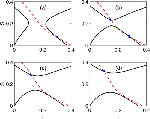
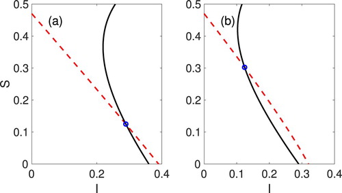
Figure A2. Graphs of $G_1(S,I)=0$ (dashed curve) and $G_2(S,I)=0$ (solid curve), given by Equations (3.10a(3.10a) $\begin{array}{rl}{G}_1(S,I)& =b(S+ϵI)\left(1-\frac{N}{\theta }\right)-hN-\alpha I=0,\end{array}$(3.10a) )–(3.10b(3.10b) $\begin{array}{rl}{G}_2(S,I)& =bϵ\left(1-\frac{N}{\theta }\right)+\frac{\beta \kappa q\gamma SN}{a(\gamma I+\mu +c)}-(\alpha +h+g)=0.\end{array}$(3.10b) ), for all of the baseline parameter values in Table 2, except for $ϵ=1$ and α. The α values and the locally stable EE (blue circle) in (a) $\alpha =0.008$, $(S^{\ast },I^{\ast })=(0.2892,0.1249)$ and (b) $\alpha =0.015$, $(S^{\ast },I^{\ast })=(0.1240,0.3023)$.

Appendix 3. Optimal control for abundance-replanting

Proof

Proof of Theorem 5.1

Corollary 4.1 of [9,17] gives the existence of an optimal control pair due to the convexity of the integrand in the objective functional with respect to the controls, a priori boundedness of the state solutions, and the Lipschitz property of the state system with respect to the state variables. Applying Pontryagin's Maximum Principle, we obtain the adjoint system given by (5.5a(5.5a) $\begin{array}{rl}\frac{\mathrm{d}{\lambda }_{1,A}}{\mathrm{d}t}& =-\left[e^{-\delta t}{p}_{1}h+{\lambda }_{1,A}\left(b\left(1-\frac{N}{\theta }\right)-\frac{bS}{\theta }-\beta W-h\right)+{\lambda }_{2,A}\left(-\frac{bϵI}{\theta }+\beta W\right)\right.\\ & \left.+{\lambda }_{3,A}\left(\frac{a{V}^2}{\kappa N^2}\right)\right],\end{array}$(5.5a) )–(5.5d(5.5d) $\begin{array}{rl}\frac{\mathrm{d}{\lambda }_{4,A}}{\mathrm{d}t}& =-\left[e^{-\delta t}(-A_3{c}^{\ast })-{\lambda }_{1,A}\beta S+{\lambda }_{2,A}\beta S+{\lambda }_{3,A}a\left(1-2\frac{V}{\kappa N}\right)-{\lambda }_{4,A}(\mu +c^{\ast })\right].\end{array}$(5.5d) ), from the defining property (A3) $\frac{\mathrm{d}{\lambda }_{1,A}}{\mathrm{d}t}=-\frac{\mathrm{d}{\mathcal{H}}_A}{\mathrm{d}S},\frac{\mathrm{d}{\lambda }_{2,A}}{\mathrm{d}t}=-\frac{\mathrm{d}{\mathcal{H}}_A}{\mathrm{d}I},\frac{\mathrm{d}{\lambda }_{3,A}}{\mathrm{d}t}=-\frac{\mathrm{d}{\mathcal{H}}_A}{\mathrm{d}U},\frac{\mathrm{d}{\lambda }_{4,A}}{\mathrm{d}t}=-\frac{\mathrm{d}{\mathcal{H}}_A}{\mathrm{d}W}.$(A3) On the interior of the set $\mathbf{U}$ we have the conditions (A4) $\begin{array}{r}\frac{\mathrm{\partial }{\mathcal{H}}_A}{\mathrm{\partial }\alpha }=0,\mathrm{a}\mathrm{t}{\mathbf{u}}_A^{\ast }=[{\alpha }_A^{\ast },c_A^{\ast }{]}^T,\end{array}$(A4) (A5) $\begin{array}{r}\frac{\mathrm{\partial }{\mathcal{H}}_A}{\mathrm{\partial }c}=0,\mathrm{a}\mathrm{t}{\mathbf{u}}_A^{\ast }=[{\alpha }_A^{\ast },c_A^{\ast }{]}^T.\end{array}$(A5) from which we can derive the equations (5.6(5.6) $\begin{array}{rl}{\alpha }_A^{\ast }\left(t\right)& =\mathrm{m}\mathrm{i}\mathrm{n}\left\{\mathrm{m}\mathrm{a}\mathrm{x}\left\{0,-\frac{A_{1}I\left(t\right)+e^{\delta t}{\lambda }_{2,A}\left(t\right)I\left(t\right)}{2A_2}\right\},{\alpha }_{max}\right\},\end{array}$(5.6) ) characterizing the optimal control.

Appendix 4. Optimal control for frequency-replanting

Theorem A.3

There exists an optimal control ${\mathbf{u}}_F^{\ast }$ and state solution of the frequency-replanting model, $X_F^{\ast }=[S_F^{\ast },I_F^{\ast },U_F^{\ast },W_F^{\ast }{]}^T$, that maximizes $J\left(\mathbf{u}\right)$ over the set $\mathbf{U}$. The associated adjoint functions ${\mathit{\lambda }}_F\left(t\right)$ with transversality (final time) conditions (A6a) $\begin{array}{rl}& {\lambda }_{1,F}\left(T\right)=1,\end{array}$(A6a) (A6b) $\begin{array}{rl}& {\lambda }_{2,F}\left(T\right)={\lambda }_{3,F}\left(T\right)={\lambda }_{4,F}\left(T\right)=0,\end{array}$(A6b) satisfy the evolution system (A7a) $\begin{array}{rl}\frac{\mathrm{d}{\lambda }_{1,F}}{\mathrm{d}t}& =-\left[e^{-\delta t}{p}_{1}h+{\lambda }_{1,F}\left\{\left(\frac{bS}{S+ϵI}\left(1-\frac{2S+I}{\theta }\right)\right)+\frac{bSϵI}{(S+ϵI{)}^2}\left(1-\frac{N}{\theta }\right)-\beta W-h\right\}\right.\\ & \left.+{\lambda }_{2,F}\left\{-\frac{bϵI^2}{\theta (S+ϵI)}-\frac{bϵI^2}{(S+ϵI{)}^2}\left(1-\frac{N}{\theta }\right)+\beta W\right\}+{\lambda }_{3,F}\left(\frac{a{V}^2}{\kappa N^2}\right)\right],\end{array}$(A7a) (A7b) $\begin{array}{rl}\frac{\mathrm{d}{\lambda }_{2,F}}{\mathrm{d}t}& =-\left[e^{-\delta t}(p_{2}h-A_1{\alpha }^{\ast })+{\lambda }_{1,F}\left\{-\frac{b{S}^2}{\theta (S+ϵI)}-\frac{bϵS^2}{(S+ϵI{)}^2}\left(1-\frac{N}{\theta }\right)+g\right\}\right.\\ & +{\lambda }_{2,F}\left\{-\frac{bϵI^2}{\theta (S+ϵI)}+bϵI\left(1-\frac{N}{\theta }\right)\left(\frac{2S+ϵI}{(S+ϵI{)}^2}\right)-(\alpha +h+g)\right\}\\ & +\left.{\lambda }_{3,F}\left(\frac{a{V}^2}{\kappa N^2}-\gamma U\right)+{\lambda }_{4,F}\gamma U\right],\end{array}$(A7b) (A7c) $\begin{array}{rl}\frac{\mathrm{d}{\lambda }_{3,F}}{\mathrm{d}t}& =-\left[e^{-\delta t}(-A_3{c}^{\ast })+{\lambda }_{3,F}\left(a\left(1-2\frac{V}{\kappa N}\right)-\gamma I-(\mu +c^{\ast })\right)+{\lambda }_{4,F}\gamma I\right],\end{array}$(A7c) (A7d) $\begin{array}{rl}\frac{\mathrm{d}{\lambda }_{4,F}}{\mathrm{d}t}& =-\left[e^{-\delta t}(-A_3{c}^{\ast })-\beta S{\lambda }_{1,F}+\beta S{\lambda }_{2,F}+{\lambda }_{3,F}a\left(1-2\frac{V}{\kappa N}\right)-(\mu +c^{\ast }){\lambda }_{4,F}\right].\end{array}$(A7d) Finally, the optimal control ${\mathbf{u}}_F^{\ast }=[{\alpha }_F^{\ast },c_F^{\ast }]$ satisfies the characterization (A8) $\begin{array}{rl}{\alpha }_F^{\ast }\left(t\right)& =\mathrm{m}\mathrm{i}\mathrm{n}\left\{\mathrm{m}\mathrm{a}\mathrm{x}\left\{0,-\frac{A_{1}I\left(t\right)+e^{\delta t}{\lambda }_{2,F}\left(t\right)I\left(t\right)}{2A_2}\right\},{\alpha }_{\mathrm{m}\mathrm{a}\mathrm{x}}\right\},\end{array}$(A8) (A9) $\begin{array}{rl}{c}_F^{\ast }\left(t\right)& =\mathrm{m}\mathrm{i}\mathrm{n}\left\{\mathrm{m}\mathrm{a}\mathrm{x}\left\{0,-\frac{A_3\left(U\right(t)+W(t\left)\right)+e^{\delta t}\left({\lambda }_{3,F}\right(t\left)U\right(t)+{\lambda }_{4,F}(t\left)W\right(t\left)\right)}{2A_4}\right\},c_{\mathrm{m}\mathrm{a}\mathrm{x}}\right\}.\end{array}$(A9)

The proof follows in a manner similar to the abundance-replanting model.

We note that the differential equations for ${\lambda }_{3,F}$ and ${\lambda }_{4,F}$ are the same as in the abundance-replanting model. In particular, since the terms involving α and c are the same in both the abundance and frequency-replanting models, the characterization of the optimal control in the frequency-replanting model is the same as in the abundance-replanting model.

References

- F. Al Basir, P.K. Roy, S. Ray, Impact of roguing and insecticides spraying on mosaic disease in Jatropha Curcas. Control Cybern. 46 (2017), pp. 325–344.
- O.J. Alabi, P.L. Kumar and R.A. Naidu, Cassava mosaic disease: A curse to food security in sub-saharan Africa, Online. APS, Net Features, 2011.
- L.J.S. Allen and G.E. Lahodny Jr, Extinction thresholds in deterministic and stochastic epidemic models, J. Biol. Dynam. 6 (2012), pp. 590–611. doi: 10.1080/17513758.2012.665502
- O. Ariyo, A.G.O. Dixon and G. Atiri, Whitefly bemisia tabaci (homoptera: Aleyrodidae) infestation on cassava genotypes grown at different ecozones in nigeria, J. Econ. Entomol. 98 (2005), pp. 611–617. doi: 10.1093/jee/98.2.611
- M.-S. Chan and M.J. Jeger, An analytical model of plant virus disease dynamics with roguing and replanting, J. Appl. Ecol. 31 (1994), pp. 413–427. doi: 10.2307/2404439
- Y. Chen and J. Yang, Global stability of an sei model for plant diseases, Math. Slovaca 66 (2016), pp. 305–311.
- D. Fargette and K. Vié, Simulation of the effects of host resistance, reversion, and cutting selection on incidence of african cassava mosaic virus and yield losses in cassava, Phytopathology 85 (1995), pp. 370–375. doi: 10.1094/Phyto-85-370
- C. Fauquet and E. Fargette, African cassava mosaic virus: etiology, epidemiology, and control, Plant Dis. 74 (1990), pp. 404–411. doi: 10.1094/PD-74-0404
- W.H. Fleming, R.W. Rishel, Deterministic and Stochastic Optimal Control (Vol. 1), Springer Science & Business Media, New York, NY, 2012.
- S. Gao, L. Xia, Y. Liu and D. Xie, A plant virus disease model with periodic environment and pulse roguing, Stud. Appl. Math. 136 (2015), pp. 357–381. doi: 10.1111/sapm.12109
- M.P. Hebert, L.J. Allen, Disease outbreaks in plant-vector-virus models with vector aggregation and dispersal. Discrete Cont. Dynam. Syst. Ser. B 21 (2016), pp. 2169–2191. doi: 10.3934/dcdsb.2016042
- J.A.P. Heesterbeek and M.G. Roberts, The type-reproduction number T in models for infectious disease control, Math. Biosci. 206 (2007), pp. 3–10. doi: 10.1016/j.mbs.2004.10.013
- F.M. Hilker, L.J. Allen, V.A. Bokil, C.J. Briggs, Z. Feng, K.A. Garrett, L.J. Gross, F.M. Hamelin, M.J. Jeger, C.A. Manore, A.G. Power, M.G. Redinbaugh, M.A. Rúa and N.J. Cunniffe, Modeling virus coinfection to inform management of maize lethal necrosis in kenya, Phytopathology 107 (2017), pp. 1095–1108.
- J. Holt, M.J. Jeger, J.M. Thresh and G.W. Otim-Nape, An epidemiological model incorporating vector population dynamics applied to African cassava mosaic virus disease, J. Appl. Ecol. 34 (1997), pp. 793–806. doi: 10.2307/2404924
- M.J. Jeger, J. Holt, F. Van Den Bosch and L.V. Madden, Epidemiology of insect-transmitted plant viruses: modelling disease dynamics and control interventions, Physiol. Entomol. 29 (2004), pp. 291–304. doi: 10.1111/j.0307-6962.2004.00394.x
- M. Jeger, L.V. Madden, F. van den Bosch, Plant virus epidemiology: applications and prospects for mathematical modelling and analysis to improve understanding and disease control. Plant Dis. 102 (2018), pp. 837–854. doi: 10.1094/PDIS-04-17-0612-FE
- M.R. Kelly Jr, J.H. Tien, M.C. Eisenberg and S. Lenhart, The impact of spatial arrangements on epidemic disease dynamics and intervention strategies, J. Biol. Dynam. 10 (2016), pp. 222–249. doi: 10.1080/17513758.2016.1156172
- V. Lakshmikantham and S. Leela, Differential and Integral Inequalities: Theory and Applications, Ordinary Differential Equations, Vol. 1, Academic Press, New York, 1969.
- J. Legg, S. Jeremiah, H. Obiero, M. Maruthi, I. Ndyetabula, G. Okao-Okuja, H. Bouwmeester, S.Bigirimana, W. Tata-Hangy, G. Gashaka, G. Mkamilo, T. Alicai and P. Lava Kumar, Comparing the regional epidemiology of the cassava mosaic and cassava brown streak virus pandemics in africa, Virus Res. 159 (2011), pp. 161–170. doi: 10.1016/j.virusres.2011.04.018
- S. Lenhart and J.T. Workman, Optimal Control Applied to Biological Models, Chapman & Hall CRC, Boca Raton, FL, 2007.
- Y. Luo, S. Gao, D. Xie and Y. Dai, A discrete plant disease model with roguing and replanting, Adv. Differ. Equ. 2015 (2015), p. 12. doi: 10.1186/s13662-014-0332-3
- A. Mallela, S. Lenhart, N.K. Vaidya, HIV-TB co-infection treatment: modeling and optimal control theory perspectives. J. Comput. Appl. Math. 307 (2016), pp. 143–161. doi: 10.1016/j.cam.2016.02.051
- S.O. Mallowa, D.K. Isutsa, A.W. Kamau and J.P. Legg, Effectiveness of phytosanitation in cassava mosaic disease management in a post-epidemic area of western kenya, ARPN J. Agr. Biol. Sci. 6 (2011), pp. 8–15.
- C.F. McQuaid, C.A. Gilligan and F. van den Bosch, Considering behaviour to ensure the success of a disease control strategy, Open Sci. 4 (2017), p. 170721.
- L.S. Pontryagin, Selected Works, Volume 4: Mathematical Theory of Optimal Processes, CRC Press, Boca Raton, 1987.
- M.G. Roberts and J.A.P. Heesterbeek, A new method to estimate the effort required to control an infectious disease, Proc. R. Soc. Lond. B 270 (2003), pp. 1359–1364. doi: 10.1098/rspb.2003.2339
- S.E. Seal, M.J. Jeger and F. Van den Bosch, Begomovirus evolution and disease management, Adv. Virus Res. 67 (2006), pp. 297–316. doi: 10.1016/S0065-3527(06)67008-5
- S.E. Seal, F. VandenBosch and M.J. Jeger, Factors influencing begomovirus evolution and their increasing global significance: implications for sustainable control, Crit. Rev. Plant Sci. 25 (2006), pp. 23–46. doi: 10.1080/07352680500365257
- R. Shi, H. Zhao and S. Tang, Global dynamic analysis of a vector-borne plant disease model, Adv. Differ. Equ. 2014 (2014), p. 59. doi: 10.1186/1687-1847-2014-59
- Z. Shuai and P. van den Driessche, Global stability of infectious disease models using lyapunov functions, SIAM J. Appl. Math. 73 (2013), pp. 1513–1532. doi: 10.1137/120876642
- J. Thresh and R. Cooter, Strategies for controlling cassava mosaic virus disease in africa, Plant Pathol.54 (2005), pp. 587–614. doi: 10.1111/j.1365-3059.2005.01282.x
- F. van den Bosch and A.M. de Roos, The dynamics of infectious diseases in orchards with roguing and replanting as control strategy, J. Math. Biol. 35 (1996), pp. 129–157. doi: 10.1007/s002850050047
- P. van den Driessche and J. Watmough, Reproduction numbers and sub-threshold endemic equilibria for compartmental models of disease transmission, Math. Biosci. 180 (2002), pp. 29–48. doi: 10.1016/S0025-5564(02)00108-6
- E. Venturino, P.K. Roy, F. Al Basir and A. Datta, A model for the control of the mosaic virus disease in jatropha curcas plantations, Energ. Ecol. Environ. 1 (2016), pp. 360–369. doi: 10.1007/s40974-016-0033-8
- X.S. Zhang, J. Holt and J. Colvin, A general model of plant-virus disease infection incorporating vector aggregation, Plant Pathol. 49 (2000), pp. 435–444. doi: 10.1046/j.1365-3059.2000.00469.x