Bifurcation analysis for a delayed SEIR epidemic model with saturated incidence and saturated treatment function

Abstract

A delayed SEIR epidemic model with saturated incidence and saturated treatment function is considered in this paper. Sufficient conditions for the existence of local Hopf bifurcation are established by regarding the possible combination of the two delays as the bifurcation parameter. General formula for the direction, period and stability of the bifurcated periodic solutions are derived by using the normal form method and the centre manifold theory. Finally, some numerical simulations are given to illustrate the obtained results.

Keywords:

• Delays
• Hopf-bifurcation
• stability
• SEIR model
• periodic solution

1. Introduction

In recent years, epidemic models have been studied by many scholars to study the dynamics of disease transmissions. Incidence rate plays an important role in the modelling of epidemic dynamics. Many epidemic models are proposed based on the bilinear incidence rate $\beta SI$ and the standard incidence rate $\frac{\beta SI}{N}$ [1, 8, 10, 11]. Capasso and Serio [4] introduced the saturated incidence rate $\frac{\beta SI}{1+\alpha I}$ which includes the behavioural change and crowding effect of the infective individuals and prevents the unboundedness of the contact rate by choosing suitable parameters. This makes the saturated incidence rate $\frac{\beta SI}{1+\alpha I}$ seems more reasonable than the bilinear incidence rate. On the other hand, most of the present epidemic models assume that the treatment rate of the infection is proportional to the number of the infective individuals. Obviously, this assumption disregards the limitation of the medical resources. Based on this, Zhang et al. [19] proposed the following SEIR epidemic model with saturated incidence and saturated treatment function: (1) $\begin{array}{rl}\frac{\mathrm{d}S(t)}{\mathrm{d}t}& =A-\frac{\beta S(t)I(t)}{1+\alpha I(t)}-\mathrm{d}S(t),\\ \frac{\mathrm{d}E(t)}{\mathrm{d}t}& =\frac{\beta S(t)I(t)}{1+\alpha I(t)})-(d+\epsilon )E(t),\\ \frac{\mathrm{d}I(t)}{\mathrm{d}t}& =\epsilon E(t)-(d+\gamma +\delta )I(t)-\frac{rI(t)}{1+kI(t)},\\ \frac{\mathrm{d}R(t)}{\mathrm{d}t}& =\delta I(t)-\mathrm{d}R(t)+\frac{rI(t)}{1+kI(t)},\end{array}$(1) where $S(t)$, $E(t)$, $I(t)$, and $R(t)$ represent the numbers of susceptible, exposed but not yet infectious, infective and recovered individuals at time t, respectively. A is the recruitment rate of the population, d is the natural death rate and γ is the death rate due to the disease. $\frac{rI}{1+kI}$ is the saturated treatment rate in which r is the maximal medical resources supplied per unit time and k is the saturation factor that measures the effect of the infected being delayed for treatment. $\frac{\beta SI}{1+\alpha I}$ is the saturated incidence rate in which α is the saturation factor that measures the inhibitory effect and β is the transmission rate. ϵ is the rate of transformation from incubation period individuals to the infective ones. δ is the natural recovery rate of the infective individuals. Zhang et al. [19] studied the stability and backward bifurcation of system (1(1) $\begin{array}{rl}\frac{\mathrm{d}S(t)}{\mathrm{d}t}& =A-\frac{\beta S(t)I(t)}{1+\alpha I(t)}-\mathrm{d}S(t),\\ \frac{\mathrm{d}E(t)}{\mathrm{d}t}& =\frac{\beta S(t)I(t)}{1+\alpha I(t)})-(d+\epsilon )E(t),\\ \frac{\mathrm{d}I(t)}{\mathrm{d}t}& =\epsilon E(t)-(d+\gamma +\delta )I(t)-\frac{rI(t)}{1+kI(t)},\\ \frac{\mathrm{d}R(t)}{\mathrm{d}t}& =\delta I(t)-\mathrm{d}R(t)+\frac{rI(t)}{1+kI(t)},\end{array}$(1) ).

In fact, many diseases have different kinds of delays when they spread, such as latent period delay [5, 6, 12, 14–16, 20] and immunity period delay [13, 18, 21]. In [12], Xue and Li analysed existence of Hopf bifurcation for a delayed SIR epidemic model with logistic growth by regarding the latent period delay of the disease as a bifurcation parameter and studied the properties of the Hopf bifurcation. In [18], Zhang et al. obtained the sufficient conditions for the linear stability and existence of Hopf bifurcation of a delayed epidemic model with a nonlinear birth in population and vertical transmission by regarding the immunity period delay of the recovered individuals as a bifurcation parameter. They also derived the explicit formulas determining the direction and stability of the Hopf bifurcation. Motivated by the work above, we consider the Hopf bifurcation of the following epidemic model with two delays: (2) $\begin{array}{rl}\frac{\mathrm{d}S(t)}{\mathrm{d}t}& =A-\frac{\beta S(t)I(t)}{1+\alpha I(t)}-\mathrm{d}S(t),\\ \frac{\mathrm{d}E(t)}{\mathrm{d}t}& =\frac{\beta S(t)I(t)}{1+\alpha I(t)}-\mathrm{d}E(t)-\epsilon E(t-{\tau }_1),\\ \frac{\mathrm{d}I(t)}{\mathrm{d}t}& =\epsilon E(t-{\tau }_1)-(d+\gamma )I(t)-\delta I(t-{\tau }_2)-\frac{rI(t-{\tau }_2)}{1+kI(t-{\tau }_2)},\\ \frac{\mathrm{d}R(t)}{\mathrm{d}t}& =\delta I(t-{\tau }_2)-\mathrm{d}R(t)+\frac{rI(t-{\tau }_2)}{1+kI(t-{\tau }_2)},\end{array}$(2) where ${\tau }_1$ is the time delay due to the latent period of the disease. ${\tau }_2$ is the time delay due to the period that the infected individuals use to move into the recovered class.

The reminder of the paper is organized as follows. In Section 2, we focus on the local stability of the endemic equilibrium and the existence of the Hopf bifurcation of system (2(2) $\begin{array}{rl}\frac{\mathrm{d}S(t)}{\mathrm{d}t}& =A-\frac{\beta S(t)I(t)}{1+\alpha I(t)}-\mathrm{d}S(t),\\ \frac{\mathrm{d}E(t)}{\mathrm{d}t}& =\frac{\beta S(t)I(t)}{1+\alpha I(t)}-\mathrm{d}E(t)-\epsilon E(t-{\tau }_1),\\ \frac{\mathrm{d}I(t)}{\mathrm{d}t}& =\epsilon E(t-{\tau }_1)-(d+\gamma )I(t)-\delta I(t-{\tau }_2)-\frac{rI(t-{\tau }_2)}{1+kI(t-{\tau }_2)},\\ \frac{\mathrm{d}R(t)}{\mathrm{d}t}& =\delta I(t-{\tau }_2)-\mathrm{d}R(t)+\frac{rI(t-{\tau }_2)}{1+kI(t-{\tau }_2)},\end{array}$(2) ). Then, we obtain explicit formulas that determine the stability and direction of the Hopf bifurcation by using the normal theory and the centre manifold theorem in Section 3. Numerical simulations are carried out in Section 4 to illustrate the main theoretical results and a brief discussion is given in the last part to conclude this work.

2. Local stability and local Hopf bifurcation

By a simple computation, we can get that if $R_0=\frac{A\beta \epsilon }{d(d+\epsilon )(d+r+\gamma +\delta )}>1$ holds, then system (2(2) $\begin{array}{rl}\frac{\mathrm{d}S(t)}{\mathrm{d}t}& =A-\frac{\beta S(t)I(t)}{1+\alpha I(t)}-\mathrm{d}S(t),\\ \frac{\mathrm{d}E(t)}{\mathrm{d}t}& =\frac{\beta S(t)I(t)}{1+\alpha I(t)}-\mathrm{d}E(t)-\epsilon E(t-{\tau }_1),\\ \frac{\mathrm{d}I(t)}{\mathrm{d}t}& =\epsilon E(t-{\tau }_1)-(d+\gamma )I(t)-\delta I(t-{\tau }_2)-\frac{rI(t-{\tau }_2)}{1+kI(t-{\tau }_2)},\\ \frac{\mathrm{d}R(t)}{\mathrm{d}t}& =\delta I(t-{\tau }_2)-\mathrm{d}R(t)+\frac{rI(t-{\tau }_2)}{1+kI(t-{\tau }_2)},\end{array}$(2) ) has a unique positive equilibrium $P_{\ast }(S_{\ast },E_{\ast },I_{\ast },R_{\ast })$, where $\begin{array}{rl}{S}_{\ast }& =\frac{(d+\epsilon )(1+\alpha I_{\ast })E_{\ast }}{\beta I_{\ast }},E_{\ast }=\frac{1}{\epsilon }[(d+\gamma +\delta )I_{\ast }+\frac{r{I}_{\ast }}{1+k{I}_{\ast }}],\\ R_{\ast }& =\frac{1}{d}[\delta I_{\ast }+\frac{r{I}_{\ast }}{1+k{I}_{\ast }}],I_{\ast }=\frac{-\overline{B}+({\overline{B}}^2-4\overline{A}\overline{C}{)}^{\frac{1}{2}}}{2\overline{A}},\end{array}$ where $\begin{array}{rl}\overline{A}& =k(d+\epsilon )(d+\gamma +\delta )(\beta +\alpha d);\\ \overline{B}& =(d+\epsilon )(d+\gamma +\delta )(\beta +d\alpha +dk)+r(d+\epsilon )(\beta +d\alpha )-Ak\beta \epsilon ;\\ \overline{C}& =d(d+\epsilon )(d+r+\gamma +\delta )-A\beta \epsilon .\end{array}$ Let $\overline{S}(t)=S(t)-S_{\ast }$, $\overline{E}(t)=E(t)-E_{\ast }$, $\overline{I}(t)=I(t)-I_{\ast }$, $\overline{R}(t)=R(t)-R_{\ast }$. Dropping the bars, system (2(2) $\begin{array}{rl}\frac{\mathrm{d}S(t)}{\mathrm{d}t}& =A-\frac{\beta S(t)I(t)}{1+\alpha I(t)}-\mathrm{d}S(t),\\ \frac{\mathrm{d}E(t)}{\mathrm{d}t}& =\frac{\beta S(t)I(t)}{1+\alpha I(t)}-\mathrm{d}E(t)-\epsilon E(t-{\tau }_1),\\ \frac{\mathrm{d}I(t)}{\mathrm{d}t}& =\epsilon E(t-{\tau }_1)-(d+\gamma )I(t)-\delta I(t-{\tau }_2)-\frac{rI(t-{\tau }_2)}{1+kI(t-{\tau }_2)},\\ \frac{\mathrm{d}R(t)}{\mathrm{d}t}& =\delta I(t-{\tau }_2)-\mathrm{d}R(t)+\frac{rI(t-{\tau }_2)}{1+kI(t-{\tau }_2)},\end{array}$(2) ) becomes (3) $\begin{array}{rl}\frac{\mathrm{d}S(t)}{\mathrm{d}t}& =a_{11}S(t)+a_{13}I(t)+f_1,\\ \frac{\mathrm{d}E(t)}{\mathrm{d}t}& =a_{21}S(t)+a_{22}E(t)+a_{23}I(t)+b_{22}E(t-{\tau }_1)+f_2,\\ \frac{\mathrm{d}I(t)}{\mathrm{d}t}& =a_{33}E(t)+b_{32}E(t-{\tau }_1)+b_{33}I(t-{\tau }_2)+f_3,\\ \frac{\mathrm{d}R(t)}{\mathrm{d}t}& =a_{44}R(t)+b_{43}I(t-{\tau }_2)+f_4,\end{array}$(3) where $\begin{array}{rl}{a}_{11}& =-(d+\frac{\beta I_{\ast }}{1+\alpha I_{\ast }}),a_{13}=-\frac{\beta S_{\ast }}{(1+\alpha I_{\ast }{)}^2},a_{21}=\frac{\beta I_{\ast }}{1+\alpha I_{\ast }},\\ a_{22}& =-d,a_{23}=\frac{\beta S_{\ast }}{(1+\alpha I_{\ast }{)}^2},a_{33}=-(d+\gamma ),a_{44}=-d,\\ b_{22}& =-\epsilon ,b_{32}=\epsilon ,b_{33}=-(\delta +\frac{R}{(1+k{I}_{\ast }{)}^2}),b_{43}=\delta +\frac{r}{(1+k{I}_{\ast }{)}^2},\end{array}$ and $\begin{array}{rl}{f}_1& =a_{14}S(t)I(t)+a_{15}{I}^2(t)+a_{16}S(t)I^2(t)+a_{17}{I}^3(t)+\cdots ,\\ f_2& =a_{24}S(t)I(t)+a_{25}{I}^2(t)+a_{26}S(t)I^2(t)+a_{27}{I}^3(t)+\cdots ,\\ f_3& =b_{34}{I}^2(t-{\tau }_2)+b_{35}{I}^3(t-{\tau }_2)+\cdots ,\\ f_4& =b_{44}{I}^2(t-{\tau }_2)+b_{45}{I}^3(t-{\tau }_2)+\cdots ,\end{array}$ with $\begin{array}{rl}{a}_{14}& =-\frac{\beta }{(1+\alpha I_{\ast }{)}^2},a_{15}=\frac{\alpha \beta S_{\ast }}{(1+\alpha I_{\ast }{)}^3},a_{16}=\frac{\alpha \beta }{(1+\alpha I_{\ast }{)}^3},a_{17}=-\frac{{\alpha }^2\beta S_{\ast }}{(1+\alpha I_{\ast }{)}^4},\\ a_{24}& =\frac{\beta }{(1+\alpha I_{\ast }{)}^2},a_{25}=-\frac{\alpha \beta S_{\ast }}{(1+\alpha I_{\ast }{)}^3},a_{26}=-\frac{\alpha \beta }{(1+\alpha I_{\ast }{)}^3},a_{27}=\frac{{\alpha }^2\beta S_{\ast }}{(1+\alpha I_{\ast }{)}^4},\\ b_{34}& =\frac{kr}{(1+k{I}_{\ast }{)}^3},b_{35}=-\frac{k^{2}r}{(1+k{I}_{\ast }{)}^4},b_{44}=-\frac{kr}{(1+k{I}_{\ast }{)}^3},b_{45}=\frac{k^{2}r}{(1+k{I}_{\ast }{)}^4}.\end{array}$ Thus, the linear system of system (3(3) $\begin{array}{rl}\frac{\mathrm{d}S(t)}{\mathrm{d}t}& =a_{11}S(t)+a_{13}I(t)+f_1,\\ \frac{\mathrm{d}E(t)}{\mathrm{d}t}& =a_{21}S(t)+a_{22}E(t)+a_{23}I(t)+b_{22}E(t-{\tau }_1)+f_2,\\ \frac{\mathrm{d}I(t)}{\mathrm{d}t}& =a_{33}E(t)+b_{32}E(t-{\tau }_1)+b_{33}I(t-{\tau }_2)+f_3,\\ \frac{\mathrm{d}R(t)}{\mathrm{d}t}& =a_{44}R(t)+b_{43}I(t-{\tau }_2)+f_4,\end{array}$(3) ) is (4) $\begin{array}{rl}\frac{\mathrm{d}S(t)}{\mathrm{d}t}& =a_{11}S(t)+a_{13}I(t),\\ \frac{\mathrm{d}E(t)}{\mathrm{d}t}& =a_{21}S(t)+a_{22}E(t)+a_{23}I(t)+b_{22}E(t-{\tau }_1),\\ \frac{\mathrm{d}I(t)}{\mathrm{d}t}& =a_{33}E(t)+b_{32}E(t-{\tau }_1)+b_{33}I(t-{\tau }_2),\\ \frac{\mathrm{d}R(t)}{\mathrm{d}t}& =a_{44}R(t)+b_{43}I(t-{\tau }_2).\end{array}$(4) The characteristic equation of system (4(4) $\begin{array}{rl}\frac{\mathrm{d}S(t)}{\mathrm{d}t}& =a_{11}S(t)+a_{13}I(t),\\ \frac{\mathrm{d}E(t)}{\mathrm{d}t}& =a_{21}S(t)+a_{22}E(t)+a_{23}I(t)+b_{22}E(t-{\tau }_1),\\ \frac{\mathrm{d}I(t)}{\mathrm{d}t}& =a_{33}E(t)+b_{32}E(t-{\tau }_1)+b_{33}I(t-{\tau }_2),\\ \frac{\mathrm{d}R(t)}{\mathrm{d}t}& =a_{44}R(t)+b_{43}I(t-{\tau }_2).\end{array}$(4) ) is (5) $\begin{array}{rl}& {\lambda }^4+A_3{\lambda }^3+A_2{\lambda }^2+A_1\lambda +A_0+(B_3{\lambda }^3+B_2{\lambda }^2+B_1\lambda +B_0){\mathrm{e}}^{-\lambda {\tau }_1}\\ & +(C_3{\lambda }^3+C_2{\lambda }^2+C_1\lambda +C_0){\mathrm{e}}^{-\lambda {\tau }_2}+(D_2{\lambda }^2+D_1\lambda +D_0){\mathrm{e}}^{-\lambda ({\tau }_1+{\tau }_2)}=0,\end{array}$(5) where $\begin{array}{rl}{A}_0& =a_{11}{a}_{22}{a}_{33}{a}_{44},\\ A_1& =-[a_{11}{a}_{22}(a_{33}+a_{44})+a_{33}{a}_{44}(a_{11}+a_{22})],\\ A_2& =a_{11}{a}_{22}+a_{33}{a}_{44}+(a_{11}+a_{22})(a_{33}+a_{44}),\\ A_3& =-(a_{11}+a_{22}+a_{33}+a_{44}),\\ B_0& =a_{44}(a_{11}{a}_{33}{b}_{22}+a_{13}{a}_{21}{b}_{32}-a_{11}{a}_{23}{b}_{32}),\\ B_1& =a_{23}{b}_{32}(a_{11}+a_{44})-a_{13}{a}_{21}{b}_{32}-b_{22}(a_{11}{a}_{33}+a_{11}{a}_{44}+a_{33}{a}_{44}),\\ B_2& =(a_{11}+a_{33}+a_{44})b_{22}-a_{23}{b}_{32},B_3=-b_{22},B_3=-b_{22},\\ C_0& =a_{11}{a}_{22}{a}_{44}{b}_{33},C_1=-b_{33}(a_{11}{a}_{22}+a_{11}{a}_{44}+a_{22}{a}_{44}),\\ C_2& =(a_{11}+a_{22}+a_{44})b_{33},C_3=-b_{33},\\ D_0& =a_{11}{a}_{44}{b}_{22}{b}_{33},D_1=-b_{22}{b}_{33}(a_{11}+a_{44}),D_2=b_{22}{b}_{33}.\end{array}$ Case 1. ${\tau }_1={\tau }_2=0$, Equation (5(5) $\begin{array}{rl}& {\lambda }^4+A_3{\lambda }^3+A_2{\lambda }^2+A_1\lambda +A_0+(B_3{\lambda }^3+B_2{\lambda }^2+B_1\lambda +B_0){\mathrm{e}}^{-\lambda {\tau }_1}\\ & +(C_3{\lambda }^3+C_2{\lambda }^2+C_1\lambda +C_0){\mathrm{e}}^{-\lambda {\tau }_2}+(D_2{\lambda }^2+D_1\lambda +D_0){\mathrm{e}}^{-\lambda ({\tau }_1+{\tau }_2)}=0,\end{array}$(5) ) becomes (6) ${\lambda }^4+A_{13}{\lambda }^3+A_{12}{\lambda }^2+A_{11}\lambda +A_{10}=0,$(6) where $\begin{array}{rl}{A}_{10}& =A_0+B_0+C_0+D_0,A_{11}=A_1+B_1+C_1+D_1,\\ A_{12}& =A_2+B_2+C_2+D_2,A_{13}=A_3+B_3+C_3.\end{array}$ Obviously, $A_{13}=\frac{\beta I_{\ast }}{1+\alpha I_{\ast }}+\frac{r}{(1+k{I}_{\ast }{)}^2}+\gamma +\delta +\epsilon +4d>0$. Let $De{t}_1=A_{13}>0$. Thus, by the Routh–Hurwithz theorem, if the condition $(H_1)$ Equations (7(7) $\begin{array}{rl}De{t}_2& =\left|\begin{array}{cc}{A}_{13}& 1\\ A_{11}& A_{12}\end{array}\right|>0,\end{array}$(7) )–(9(9) $\begin{array}{rl}De{t}_4& =\left|\begin{array}{cccc}{A}_{13}& 1& 0& 0\\ A_{11}& A_{12}& A_{13}& 1\\ 0& A_{10}& A_{11}& A_{12}\\ 0& 0& 0& A_{10}\end{array}\right|>0.\end{array}$(9) ) holds, then the positive equilibrium $P_{\ast }(S_{\ast },E_{\ast },I_{\ast },R_{\ast })$ of system (2(2) $\begin{array}{rl}\frac{\mathrm{d}S(t)}{\mathrm{d}t}& =A-\frac{\beta S(t)I(t)}{1+\alpha I(t)}-\mathrm{d}S(t),\\ \frac{\mathrm{d}E(t)}{\mathrm{d}t}& =\frac{\beta S(t)I(t)}{1+\alpha I(t)}-\mathrm{d}E(t)-\epsilon E(t-{\tau }_1),\\ \frac{\mathrm{d}I(t)}{\mathrm{d}t}& =\epsilon E(t-{\tau }_1)-(d+\gamma )I(t)-\delta I(t-{\tau }_2)-\frac{rI(t-{\tau }_2)}{1+kI(t-{\tau }_2)},\\ \frac{\mathrm{d}R(t)}{\mathrm{d}t}& =\delta I(t-{\tau }_2)-\mathrm{d}R(t)+\frac{rI(t-{\tau }_2)}{1+kI(t-{\tau }_2)},\end{array}$(2) ) without time delay is locally asymptotically stable: (7) $\begin{array}{rl}De{t}_2& =\left|\begin{array}{cc}{A}_{13}& 1\\ A_{11}& A_{12}\end{array}\right|>0,\end{array}$(7) (8) $\begin{array}{rl}De{t}_3& =\left|\begin{array}{ccc}{A}_{13}& 1& 0\\ A_{11}& A_{12}& A_{13}\\ 0& A_{10}& A_{11}\end{array}\right|>0,\end{array}$(8) (9) $\begin{array}{rl}De{t}_4& =\left|\begin{array}{cccc}{A}_{13}& 1& 0& 0\\ A_{11}& A_{12}& A_{13}& 1\\ 0& A_{10}& A_{11}& A_{12}\\ 0& 0& 0& A_{10}\end{array}\right|>0.\end{array}$(9) Case 2. ${\tau }_1>0$, ${\tau }_2=0$. When ${\tau }_2=0$, Equation (5(5) $\begin{array}{rl}& {\lambda }^4+A_3{\lambda }^3+A_2{\lambda }^2+A_1\lambda +A_0+(B_3{\lambda }^3+B_2{\lambda }^2+B_1\lambda +B_0){\mathrm{e}}^{-\lambda {\tau }_1}\\ & +(C_3{\lambda }^3+C_2{\lambda }^2+C_1\lambda +C_0){\mathrm{e}}^{-\lambda {\tau }_2}+(D_2{\lambda }^2+D_1\lambda +D_0){\mathrm{e}}^{-\lambda ({\tau }_1+{\tau }_2)}=0,\end{array}$(5) ) becomes (10) ${\lambda }^4+A_{23}{\lambda }^3+A_{22}{\lambda }^2+A_{21}\lambda +A_{20}+(B_{23}{\lambda }^3+B_{22}{\lambda }^2+B_{21}\lambda +B_{20}){\mathrm{e}}^{-\lambda {\tau }_1}=0,$(10) where $\begin{array}{rl}{A}_{20}& =A_0+C_0,A_{21}=A_1+C_1,A_{22}=A_2+C_2,A_{23}=A_3+C_3,\\ B_{20}& =B_0+D_0,B_{21}=B_1+D_1,B_{22}=B_2+D_2,B_{23}=B_3.\end{array}$ Let $\lambda =\mathrm{i}{\omega }_1({\omega }_1>0)$ be the root of Equation (10(10) ${\lambda }^4+A_{23}{\lambda }^3+A_{22}{\lambda }^2+A_{21}\lambda +A_{20}+(B_{23}{\lambda }^3+B_{22}{\lambda }^2+B_{21}\lambda +B_{20}){\mathrm{e}}^{-\lambda {\tau }_1}=0,$(10) ), then (11) $\begin{array}{rl}& (B_{21}{\omega }_1-B_{23}{\omega }_1^3)\sin {\tau }_1{\omega }_1+(B_{20}-B_{22}{\omega }_1^2)\cos {\tau }_1{\omega }_1=A_{22}{\omega }_1^2-{\omega }_1^4-A_{20},\\ & (B_{21}{\omega }_1-B_{23}{\omega }_1^3)\cos {\tau }_1{\omega }_1-(B_{20}-B_{22}{\omega }_1^2)\sin {\tau }_1{\omega }_1=A_{23}{\omega }_1^3-A_{21}{\omega }_1,\end{array}$(11) from which one can get (12) ${\omega }_1^8+e_{23}{\omega }_1^6+e_{22}{\omega }_1^4+e_{21}{\omega }_1^2+e_{20}=0,$(12) with $\begin{array}{rl}{e}_{20}& =A_{20}^2-B_{20}^2,e_{21}=A_{21}^2-B_{21}^2-2A_{20}{A}_{22}+2B_{20}{B}_{22},\\ e_{22}& =A_{22}^2-B_{22}^2+2A_{20}-2A_{21}{A}_{23}+2B_{21}{B}_{23},e_{23}=A_{23}^2-B_{23}^2-2A_{22}.\end{array}$ Let ${\omega }_1^2=v_1$, then Equation (12(12) ${\omega }_1^8+e_{23}{\omega }_1^6+e_{22}{\omega }_1^4+e_{21}{\omega }_1^2+e_{20}=0,$(12) ) becomes (13) $v_1^4+e_{23}{v}_1^3+e_{22}{v}_1^2+e_{21}{v}_1+e_{20}=0.$(13) Discussion about the roots of Equation (13(13) $v_1^4+e_{23}{v}_1^3+e_{22}{v}_1^2+e_{21}{v}_1+e_{20}=0.$(13) ) is similar to that in [9]. Thus, in order to obtain the main results in this paper, we make the following assumption.

$(H_{21})$ Equation (13(13) $v_1^4+e_{23}{v}_1^3+e_{22}{v}_1^2+e_{21}{v}_1+e_{20}=0.$(13) ) has at least one positive root.

Then, there exists a positive root of Equation (13(13) $v_1^4+e_{23}{v}_1^3+e_{22}{v}_1^2+e_{21}{v}_1+e_{20}=0.$(13) ) $v_{10}$ such that Equation (10(10) ${\lambda }^4+A_{23}{\lambda }^3+A_{22}{\lambda }^2+A_{21}\lambda +A_{20}+(B_{23}{\lambda }^3+B_{22}{\lambda }^2+B_{21}\lambda +B_{20}){\mathrm{e}}^{-\lambda {\tau }_1}=0,$(10) ) has a pair of purely imaginary roots $\pm \mathrm{i}{\omega }_{10}=\pm \mathrm{i}\sqrt{v_{10}}$. Then, from Equation (11(11) $\begin{array}{rl}& (B_{21}{\omega }_1-B_{23}{\omega }_1^3)\sin {\tau }_1{\omega }_1+(B_{20}-B_{22}{\omega }_1^2)\cos {\tau }_1{\omega }_1=A_{22}{\omega }_1^2-{\omega }_1^4-A_{20},\\ & (B_{21}{\omega }_1-B_{23}{\omega }_1^3)\cos {\tau }_1{\omega }_1-(B_{20}-B_{22}{\omega }_1^2)\sin {\tau }_1{\omega }_1=A_{23}{\omega }_1^3-A_{21}{\omega }_1,\end{array}$(11) ), we can obtain the corresponding critical value of the delay for ${\omega }_{10}$ (14) ${\tau }_{10}=\frac{1}{{\omega }_{10}}\arccos \frac{h_{26}{\omega }_{10}^6+h_{24}{\omega }_{10}^4+h_{22}{\omega }_{10}^2+h_{20}}{g_{26}{\omega }_{10}^6+g_{24}{\omega }_{10}^4+g_{22}{\omega }_{10}^2+g_{20}},$(14) where $\begin{array}{rl}{g}_{20}& =B_{20}^2,g_{22}=B_{21}^2-2B_{20}{B}_{22},g_{24}=B_{22}^2-2B_{21}{B}_{23},g_{26}=B_{23}^2,\\ h_{20}& =-A_{20}{B}_{20},h_{22}=A_{20}{B}_{22}-A_{21}{B}_{21}+A_{22}{B}_{20},\\ h_{24}& =A_{21}{B}_{23}-A_{22}{B}_{22}+A_{23}{B}_{21}-B_{20},h_{26}=B_{22}-A_{23}{B}_{23}.\end{array}$ Substituting $\lambda ({\tau }_1)$ into Equation (10(10) ${\lambda }^4+A_{23}{\lambda }^3+A_{22}{\lambda }^2+A_{21}\lambda +A_{20}+(B_{23}{\lambda }^3+B_{22}{\lambda }^2+B_{21}\lambda +B_{20}){\mathrm{e}}^{-\lambda {\tau }_1}=0,$(10) ) and taking the derivative with respect to ${\tau }_1$, we get $\begin{array}{rl}[\frac{\mathrm{d}\lambda }{\mathrm{d}{\tau }_1}{]}^{-1}& =-\frac{4{\lambda }^3+3A_{23}{\lambda }^2+2A_{22}\lambda +A_{21}}{\lambda ({\lambda }^4+A_{23}{\lambda }^3+A_{22}{\lambda }^2+A_{21}\lambda +A_{20})}\\ & +\frac{3B_{23}{\lambda }^2+2B_{22}\lambda +B_{21}}{\lambda (B_{23}{\lambda }^3+B_{22}{\lambda }^2+B_{21}\lambda +B_{20})}-\frac{{\tau }_1}{\lambda },\end{array}$ which leads to $\mathrm{Re}[\frac{\mathrm{d}\lambda }{\mathrm{d}{\tau }_1}{]}_{{\tau }_1={\tau }_{10}}^{-1}=\frac{f_1^{\mathrm{\prime }}(v_{1\ast })}{(B_{21}{\omega }_{10}-B_{23}{\omega }_{10}^3{)}^2+(B_{20}-B_{22}{\omega }_{10}^2{)}^2},$ where $f_1(v_1)=v_1^4+e_{23}{v}_1^3+e_{22}{v}_1^2+e_{21}{v}_1+e_{20}$ and $v_{1\ast }={\omega }_{10}^2$. Thus, if the condition $(H_{22})$ $f_1^{\mathrm{\prime }}(v_{1\ast })\ne 0$ holds, then $\mathrm{Re}[\frac{\mathrm{d}\lambda }{\mathrm{d}{\tau }_1}{]}_{{\tau }_1={\tau }_{10}}^{-1}\ne 0$. According to the Hopf bifurcation theorem in [18], we have the following for system (2(2) $\begin{array}{rl}\frac{\mathrm{d}S(t)}{\mathrm{d}t}& =A-\frac{\beta S(t)I(t)}{1+\alpha I(t)}-\mathrm{d}S(t),\\ \frac{\mathrm{d}E(t)}{\mathrm{d}t}& =\frac{\beta S(t)I(t)}{1+\alpha I(t)}-\mathrm{d}E(t)-\epsilon E(t-{\tau }_1),\\ \frac{\mathrm{d}I(t)}{\mathrm{d}t}& =\epsilon E(t-{\tau }_1)-(d+\gamma )I(t)-\delta I(t-{\tau }_2)-\frac{rI(t-{\tau }_2)}{1+kI(t-{\tau }_2)},\\ \frac{\mathrm{d}R(t)}{\mathrm{d}t}& =\delta I(t-{\tau }_2)-\mathrm{d}R(t)+\frac{rI(t-{\tau }_2)}{1+kI(t-{\tau }_2)},\end{array}$(2) ).

Theorem 2.1

If the conditions $(H_{21})$–$(H_{22})$ hold, then

1. the positive equilibrium $P_{\ast }(S_{\ast },E_{\ast },I_{\ast },R_{\ast })$ of system (2(2) $\begin{array}{rl}\frac{\mathrm{d}S(t)}{\mathrm{d}t}& =A-\frac{\beta S(t)I(t)}{1+\alpha I(t)}-\mathrm{d}S(t),\\ \frac{\mathrm{d}E(t)}{\mathrm{d}t}& =\frac{\beta S(t)I(t)}{1+\alpha I(t)}-\mathrm{d}E(t)-\epsilon E(t-{\tau }_1),\\ \frac{\mathrm{d}I(t)}{\mathrm{d}t}& =\epsilon E(t-{\tau }_1)-(d+\gamma )I(t)-\delta I(t-{\tau }_2)-\frac{rI(t-{\tau }_2)}{1+kI(t-{\tau }_2)},\\ \frac{\mathrm{d}R(t)}{\mathrm{d}t}& =\delta I(t-{\tau }_2)-\mathrm{d}R(t)+\frac{rI(t-{\tau }_2)}{1+kI(t-{\tau }_2)},\end{array}$(2) ) is asymptotically stable for ${\tau }_1\in [0,{\tau }_{10})$;

2. system (2(2) $\begin{array}{rl}\frac{\mathrm{d}S(t)}{\mathrm{d}t}& =A-\frac{\beta S(t)I(t)}{1+\alpha I(t)}-\mathrm{d}S(t),\\ \frac{\mathrm{d}E(t)}{\mathrm{d}t}& =\frac{\beta S(t)I(t)}{1+\alpha I(t)}-\mathrm{d}E(t)-\epsilon E(t-{\tau }_1),\\ \frac{\mathrm{d}I(t)}{\mathrm{d}t}& =\epsilon E(t-{\tau }_1)-(d+\gamma )I(t)-\delta I(t-{\tau }_2)-\frac{rI(t-{\tau }_2)}{1+kI(t-{\tau }_2)},\\ \frac{\mathrm{d}R(t)}{\mathrm{d}t}& =\delta I(t-{\tau }_2)-\mathrm{d}R(t)+\frac{rI(t-{\tau }_2)}{1+kI(t-{\tau }_2)},\end{array}$(2) ) undergoes a Hopf bifurcation at the positive equilibrium $P_{\ast }(S_{\ast },E_{\ast },I_{\ast },R_{\ast })$ when ${\tau }_1={\tau }_{10}$.

${\tau }_{10}$ is defined as in Equation (14(14) ${\tau }_{10}=\frac{1}{{\omega }_{10}}\arccos \frac{h_{26}{\omega }_{10}^6+h_{24}{\omega }_{10}^4+h_{22}{\omega }_{10}^2+h_{20}}{g_{26}{\omega }_{10}^6+g_{24}{\omega }_{10}^4+g_{22}{\omega }_{10}^2+g_{20}},$(14) ).

Case 3. ${\tau }_1=0$, ${\tau }_2>0$. When ${\tau }_1=0$, Equation (5(5) $\begin{array}{rl}& {\lambda }^4+A_3{\lambda }^3+A_2{\lambda }^2+A_1\lambda +A_0+(B_3{\lambda }^3+B_2{\lambda }^2+B_1\lambda +B_0){\mathrm{e}}^{-\lambda {\tau }_1}\\ & +(C_3{\lambda }^3+C_2{\lambda }^2+C_1\lambda +C_0){\mathrm{e}}^{-\lambda {\tau }_2}+(D_2{\lambda }^2+D_1\lambda +D_0){\mathrm{e}}^{-\lambda ({\tau }_1+{\tau }_2)}=0,\end{array}$(5) ) becomes (15) ${\lambda }^4+A_{33}{\lambda }^3+A_{32}{\lambda }^2+A_{31}\lambda +A_{30}+(B_{33}{\lambda }^3+B_{32}{\lambda }^2+B_{31}\lambda +B_{30}){\mathrm{e}}^{-\lambda {\tau }_2}=0,$(15) where $\begin{array}{rl}{A}_{30}& =A_0+B_0,A_{31}=A_1+B_1,A_{32}=A_2+B_2,A_{33}=A_3+B_3,\\ B_{30}& =C_0+D_0,B_{31}=C_1+D_1,B_{32}=C_2+D_2,B_{33}=C_3.\end{array}$ Let $\lambda =\mathrm{i}{\omega }_2({\omega }_2>0)$ be the root of Equation (15(15) ${\lambda }^4+A_{33}{\lambda }^3+A_{32}{\lambda }^2+A_{31}\lambda +A_{30}+(B_{33}{\lambda }^3+B_{32}{\lambda }^2+B_{31}\lambda +B_{30}){\mathrm{e}}^{-\lambda {\tau }_2}=0,$(15) ), then (16) $\begin{array}{rl}& (B_{31}{\omega }_2-B_{33}{\omega }_2^3)\sin {\tau }_2{\omega }_2+(B_{30}-B_{32}{\omega }_2^2)\cos {\tau }_2{\omega }_2=A_{32}{\omega }_2^2-{\omega }_2^4-A_{30},\\ & (B_{31}{\omega }_2-B_{33}{\omega }_2^3)\cos {\tau }_2{\omega }_2-(B_{30}-B_{32}{\omega }_2^2)\sin {\tau }_2{\omega }_2=A_{33}{\omega }_2^3-A_{31}{\omega }_2,\end{array}$(16) from which one can get (17) ${\omega }_2^8+e_{33}{\omega }_2^6+e_{32}{\omega }_2^4+e_{31}{\omega }_2^2+e_{30}=0,$(17) with $\begin{array}{rl}{e}_{30}& =A_{30}^2-B_{30}^2,e_{31}=A_{31}^2-B_{31}^2-2A_{30}{A}_{32}+2B_{30}{B}_{32},\\ e_{32}& =A_{32}^2-B_{32}^2+2A_{30}-2A_{31}{A}_{33}+2B_{31}{B}_{33},e_{33}=A_{33}^2-B_{33}^2-2A_{32}.\end{array}$ Let ${\omega }_2^2=v_2$, then Equation (17(17) ${\omega }_2^8+e_{33}{\omega }_2^6+e_{32}{\omega }_2^4+e_{31}{\omega }_2^2+e_{30}=0,$(17) ) becomes (18) $v_2^4+e_{33}{v}_2^3+e_{32}{v}_2^2+e_{31}{v}_2+e_{30}=0.$(18) Similar as in Case 2, we can make the following assumption.

$(H_{31})$ Equation (18(18) $v_2^4+e_{33}{v}_2^3+e_{32}{v}_2^2+e_{31}{v}_2+e_{30}=0.$(18) ) has at least one positive root.

Then there exists a positive root of Equation (18(18) $v_2^4+e_{33}{v}_2^3+e_{32}{v}_2^2+e_{31}{v}_2+e_{30}=0.$(18) ) such that Equation (15(15) ${\lambda }^4+A_{33}{\lambda }^3+A_{32}{\lambda }^2+A_{31}\lambda +A_{30}+(B_{33}{\lambda }^3+B_{32}{\lambda }^2+B_{31}\lambda +B_{30}){\mathrm{e}}^{-\lambda {\tau }_2}=0,$(15) ) has a pair of purely imaginary roots $\pm \mathrm{i}{\omega }_{20}=\pm \mathrm{i}\sqrt{v_{20}}$. Then, from Equation (16(16) $\begin{array}{rl}& (B_{31}{\omega }_2-B_{33}{\omega }_2^3)\sin {\tau }_2{\omega }_2+(B_{30}-B_{32}{\omega }_2^2)\cos {\tau }_2{\omega }_2=A_{32}{\omega }_2^2-{\omega }_2^4-A_{30},\\ & (B_{31}{\omega }_2-B_{33}{\omega }_2^3)\cos {\tau }_2{\omega }_2-(B_{30}-B_{32}{\omega }_2^2)\sin {\tau }_2{\omega }_2=A_{33}{\omega }_2^3-A_{31}{\omega }_2,\end{array}$(16) ), we can obtain the corresponding critical value of the delay for ${\omega }_{20}$ (19) ${\tau }_{20}=\frac{1}{{\omega }_{20}}\arccos \frac{h_{36}{\omega }_{20}^6+h_{34}{\omega }_{20}^4+h_{32}{\omega }_{20}^2+h_{30}}{g_{36}{\omega }_{20}^6+g_{34}{\omega }_{20}^4+g_{32}{\omega }_{20}^2+g_{30}},$(19) where $\begin{array}{rl}{g}_{30}& =B_{30}^2,g_{32}=B_{31}^2-2B_{30}{B}_{32},g_{34}=B_{32}^2-2B_{31}{B}_{33},g_{36}=B_{33}^2,\\ h_{30}& =-A_{30}{B}_{30},h_{32}=A_{30}{B}_{32}-A_{31}{B}_{31}+A_{32}{B}_{30},\\ h_{34}& =A_{31}{B}_{33}-A_{32}{B}_{32}+A_{33}{B}_{31}-B_{30},h_{36}=B_{32}-A_{33}{B}_{33}.\end{array}$ Then, we can get $\begin{array}{rl}[\frac{\mathrm{d}\lambda }{\mathrm{d}{\tau }_2}{]}^{-1}& =-\frac{4{\lambda }^3+3A_{33}{\lambda }^2+2A_{32}\lambda +A_{31}}{\lambda ({\lambda }^4+A_{33}{\lambda }^3+A_{32}{\lambda }^2+A_{31}\lambda +A_{30})}\\ & +\frac{3B_{33}{\lambda }^2+2B_{32}\lambda +B_{31}}{\lambda (B_{33}{\lambda }^3+B_{32}{\lambda }^2+B_{31}\lambda +B_{30})}-\frac{{\tau }_2}{\lambda },\end{array}$ which leads to $\mathrm{Re}[\frac{\mathrm{d}\lambda }{\mathrm{d}{\tau }_2}{]}_{{\tau }_2={\tau }_{20}}^{-1}=\frac{f_2^{\mathrm{\prime }}(v_{2\ast })}{(B_{31}{\omega }_{20}-B_{33}{\omega }_{20}^3{)}^2+(B_{30}-B_{32}{\omega }_{20}^2{)}^2},$ where $f_2(v_2)=v_2^4+e_{33}{v}_2^3+e_{32}{v}_2^2+e_{31}{v}_2+e_{30}$ and $v_{2\ast }={\omega }_{20}^2$. Thus, if the condition $(H_{32})$ $f_2^{\mathrm{\prime }}(v_{2\ast })\ne 0$ holds, then $\mathrm{Re}[\frac{\mathrm{d}\lambda }{\mathrm{d}{\tau }_2}{]}_{{\tau }_2={\tau }_{20}}^{-1}\ne 0$. According to the Hopf bifurcation theorem in [18], we have the following for system (2(2) $\begin{array}{rl}\frac{\mathrm{d}S(t)}{\mathrm{d}t}& =A-\frac{\beta S(t)I(t)}{1+\alpha I(t)}-\mathrm{d}S(t),\\ \frac{\mathrm{d}E(t)}{\mathrm{d}t}& =\frac{\beta S(t)I(t)}{1+\alpha I(t)}-\mathrm{d}E(t)-\epsilon E(t-{\tau }_1),\\ \frac{\mathrm{d}I(t)}{\mathrm{d}t}& =\epsilon E(t-{\tau }_1)-(d+\gamma )I(t)-\delta I(t-{\tau }_2)-\frac{rI(t-{\tau }_2)}{1+kI(t-{\tau }_2)},\\ \frac{\mathrm{d}R(t)}{\mathrm{d}t}& =\delta I(t-{\tau }_2)-\mathrm{d}R(t)+\frac{rI(t-{\tau }_2)}{1+kI(t-{\tau }_2)},\end{array}$(2) ).

Theorem 2.2

If the conditions $(H_{31})$–$(H_{32})$ hold, then

1. the positive equilibrium $P_{\ast }(S_{\ast },E_{\ast },I_{\ast },R_{\ast })$ of system (2(2) $\begin{array}{rl}\frac{\mathrm{d}S(t)}{\mathrm{d}t}& =A-\frac{\beta S(t)I(t)}{1+\alpha I(t)}-\mathrm{d}S(t),\\ \frac{\mathrm{d}E(t)}{\mathrm{d}t}& =\frac{\beta S(t)I(t)}{1+\alpha I(t)}-\mathrm{d}E(t)-\epsilon E(t-{\tau }_1),\\ \frac{\mathrm{d}I(t)}{\mathrm{d}t}& =\epsilon E(t-{\tau }_1)-(d+\gamma )I(t)-\delta I(t-{\tau }_2)-\frac{rI(t-{\tau }_2)}{1+kI(t-{\tau }_2)},\\ \frac{\mathrm{d}R(t)}{\mathrm{d}t}& =\delta I(t-{\tau }_2)-\mathrm{d}R(t)+\frac{rI(t-{\tau }_2)}{1+kI(t-{\tau }_2)},\end{array}$(2) ) is asymptotically stable for ${\tau }_2\in [0,{\tau }_{20})$;

2. system (2(2) $\begin{array}{rl}\frac{\mathrm{d}S(t)}{\mathrm{d}t}& =A-\frac{\beta S(t)I(t)}{1+\alpha I(t)}-\mathrm{d}S(t),\\ \frac{\mathrm{d}E(t)}{\mathrm{d}t}& =\frac{\beta S(t)I(t)}{1+\alpha I(t)}-\mathrm{d}E(t)-\epsilon E(t-{\tau }_1),\\ \frac{\mathrm{d}I(t)}{\mathrm{d}t}& =\epsilon E(t-{\tau }_1)-(d+\gamma )I(t)-\delta I(t-{\tau }_2)-\frac{rI(t-{\tau }_2)}{1+kI(t-{\tau }_2)},\\ \frac{\mathrm{d}R(t)}{\mathrm{d}t}& =\delta I(t-{\tau }_2)-\mathrm{d}R(t)+\frac{rI(t-{\tau }_2)}{1+kI(t-{\tau }_2)},\end{array}$(2) ) undergoes a Hopf bifurcation at the positive equilibrium $P_{\ast }(S_{\ast },E_{\ast },I_{\ast },R_{\ast })$ when ${\tau }_2={\tau }_{20}$.

${\tau }_{20}$ is defined as in Equation (19(19) ${\tau }_{20}=\frac{1}{{\omega }_{20}}\arccos \frac{h_{36}{\omega }_{20}^6+h_{34}{\omega }_{20}^4+h_{32}{\omega }_{20}^2+h_{30}}{g_{36}{\omega }_{20}^6+g_{34}{\omega }_{20}^4+g_{32}{\omega }_{20}^2+g_{30}},$(19) ).

Case 4. ${\tau }_1={\tau }_2=\tau >0$. When ${\tau }_1={\tau }_2=\tau$, Equation (5(5) $\begin{array}{rl}& {\lambda }^4+A_3{\lambda }^3+A_2{\lambda }^2+A_1\lambda +A_0+(B_3{\lambda }^3+B_2{\lambda }^2+B_1\lambda +B_0){\mathrm{e}}^{-\lambda {\tau }_1}\\ & +(C_3{\lambda }^3+C_2{\lambda }^2+C_1\lambda +C_0){\mathrm{e}}^{-\lambda {\tau }_2}+(D_2{\lambda }^2+D_1\lambda +D_0){\mathrm{e}}^{-\lambda ({\tau }_1+{\tau }_2)}=0,\end{array}$(5) ) becomes (20) $\begin{array}{rl}& {\lambda }^4+A_{43}{\lambda }^3+A_{42}{\lambda }^2+A_{41}\lambda +A_{40}+(B_{43}{\lambda }^3+B_{42}{\lambda }^2+B_{41}\lambda +B_{40}){\mathrm{e}}^{-\lambda \tau }\\ & +(C_{42}{\lambda }^2+C_{41}\lambda +C_{40}){\mathrm{e}}^{-2\lambda \tau }=0,\end{array}$(20) where $\begin{array}{rl}{A}_{40}& =A_0,A_{41}=A_1,A_{42}=A_2,A_{43}=A_3,\\ B_{40}& =B_0+C_0,B_{41}=B_1+C_1,B_{42}=B_2+C_2,B_{43}=B_3+C_3,\\ C_{40}& =D_1,C_{41}=D_1,C_{42}=D_2.\end{array}$ Multiplying ${\mathrm{e}}^{\lambda \tau }$ on both sides of Equation (20(20) $\begin{array}{rl}& {\lambda }^4+A_{43}{\lambda }^3+A_{42}{\lambda }^2+A_{41}\lambda +A_{40}+(B_{43}{\lambda }^3+B_{42}{\lambda }^2+B_{41}\lambda +B_{40}){\mathrm{e}}^{-\lambda \tau }\\ & +(C_{42}{\lambda }^2+C_{41}\lambda +C_{40}){\mathrm{e}}^{-2\lambda \tau }=0,\end{array}$(20) ), we can get (21) $\begin{array}{rl}& B_{43}{\lambda }^3+B_{42}{\lambda }^2+B_{41}\lambda +B_{40}+({\lambda }^4+A_{43}{\lambda }^3+A_{42}{\lambda }^2+A_{41}\lambda +A_{40}){\mathrm{e}}^{\lambda \tau }\\ & +(C_{42}{\lambda }^2+C_{41}\lambda +C_{40}){\mathrm{e}}^{-\lambda \tau }=0.\end{array}$(21) Let $\lambda =\mathrm{i}\omega (\omega >0)$ be the root of Equation (21(21) $\begin{array}{rl}& B_{43}{\lambda }^3+B_{42}{\lambda }^2+B_{41}\lambda +B_{40}+({\lambda }^4+A_{43}{\lambda }^3+A_{42}{\lambda }^2+A_{41}\lambda +A_{40}){\mathrm{e}}^{\lambda \tau }\\ & +(C_{42}{\lambda }^2+C_{41}\lambda +C_{40}){\mathrm{e}}^{-\lambda \tau }=0.\end{array}$(21) ), then (22) $\begin{array}{rl}& M_{41}(\omega )\cos \tau \omega -M_{42}(\omega )\sin \tau \omega =M_{43}(\omega ),\\ & M_{44}(\omega )\sin \tau \omega +M_{45}(\omega )\cos \tau \omega =M_{46}(\omega ),\end{array}$(22) where $\begin{array}{rl}{M}_{41}(\omega )& ={\omega }^4-(A_{42}+C_{42}){\omega }^2+A_{40}+C_{40},\\ M_{42}(\omega )& =(A_{41}-C_{41})\omega -A_{43}{\omega }^3,\\ M_{43}(\omega )& =B_{42}{\omega }^2-B_{40},\\ M_{44}(\omega )& ={\omega }^4-(A_{42}-C_{42}){\omega }^2+A_{40}-C_{40},\\ M_{45}(\omega )& =(A_{41}+C_{41})\omega -A_{43}{\omega }^3,\\ M_{46}(\omega )& =B_{43}{\omega }^3-B_{41}\omega .\end{array}$ From Equation (23(23) ${\omega }^{16}+e_{47}{\omega }^{14}+e_{46}{\omega }^{12}+e_{45}{\omega }^{10}+e_{44}{\omega }^8+e_{43}{\omega }^6+e_{42}{\omega }^4+e_{41}{\omega }^2+e_{40}=0,$(23) ), we get $\begin{array}{rl}\cos \tau \omega & =\frac{p_6{\omega }^6+p_4{\omega }^4+p_2{\omega }^2+p_0}{{\omega }^8+q_6{\omega }^6+q_4{\omega }^4+q_2{\omega }^2+q_0},\\ \sin \tau \omega & =\frac{p_7{\omega }^7+p_5{\omega }^5+p_3{\omega }^3+p_1\omega }{{\omega }^8+q_6{\omega }^6+q_4{\omega }^4+q_2{\omega }^2+q_0},\end{array}$ with $\begin{array}{rl}{p}_0& =B_{40}(C_{40}-A_{40}),p_1=B_{40}(A_{41}+C_{41})-B_{41}(A_{40}+C_{40}),\\ p_2& =B_{40}(A_{42}-C_{42})-B_{41}(A_{41}-C_{41})+B_{42}(A_{40}-C_{40}),\\ p_3& =B_{41}(A_{42}+C_{42})+B_{43}(A_{40}+C_{40})-B_{42}(A_{41}+C_{41})-A_{43}{B}_{40},\\ p_4& =A_{43}{B}_{41}-B_{40}-B_{42}(A_{42}-C_{42})+B_{43}(A_{41}-C_{41}),\\ p_5& =A_{43}{B}_{42}-B_{41}-B_{43}(A_{42}+C_{42}),p_6=B_{42}-A_{43}{B}_{43},p_7=B_{43},\\ q_0& =A_{40}^2-C_{40}^2,q_2=A_{41}^2-C_{41}^2-2A_{40}{A}_{42}+2C_{40}{C}_{42},\\ q_4& =A_{42}^2-C_{42}^2+2A_{40}-2A_{41}{A}_{43},q_6=A_{43}^2-2A_{42}.\end{array}$ Thus, we have (23) ${\omega }^{16}+e_{47}{\omega }^{14}+e_{46}{\omega }^{12}+e_{45}{\omega }^{10}+e_{44}{\omega }^8+e_{43}{\omega }^6+e_{42}{\omega }^4+e_{41}{\omega }^2+e_{40}=0,$(23) where $\begin{array}{rl}{e}_{40}& =q_0^2-p_0^2,e_{41}=2q_0{q}_2-2p_0{p}_2-p_1^2,\\ e_{42}& =q_2^2-p_2^2+2q_0{q}_4-2p_0{p}_4-2p_1{p}_3,\\ e_{43}& =2q_0{q}_6+2q_2{q}_4-2p_0{p}_6-2p_1{p}_5-2p_2{p}_4-p_3^2,\\ e_{44}& =q_4^2-p_4^2+2q_0+2q_2{q}_6-2p_1{p}_7-2p_2{p}_6-2p_3{p}_5,\\ e_{45}& =2q_2+2q_4{q}_6-2p_4{p}_6-p_5^2-2p_3{p}_7,\\ e_{46}& =q_6^2+2q_4-p_6^2-2p_5{p}_7,e_{47}=2q_6-p_7^2.\end{array}$ Let ${\omega }^2=v$, then Equation (23(23) ${\omega }^{16}+e_{47}{\omega }^{14}+e_{46}{\omega }^{12}+e_{45}{\omega }^{10}+e_{44}{\omega }^8+e_{43}{\omega }^6+e_{42}{\omega }^4+e_{41}{\omega }^2+e_{40}=0,$(23) ) becomes (24) $v^8+e_{47}{v}^7+e_{46}{v}^6+e_{45}{v}^5+e_{44}{v}^4+e_{43}{v}^3+e_{42}{v}^2+e_{41}v+e_{40}=0.$(24) Next, we make the following assumption.

$(H_{42})$ Equation (24(24) $v^8+e_{47}{v}^7+e_{46}{v}^6+e_{45}{v}^5+e_{44}{v}^4+e_{43}{v}^3+e_{42}{v}^2+e_{41}v+e_{40}=0.$(24) ) has at least one positive root.

Then, Equation (24(24) $v^8+e_{47}{v}^7+e_{46}{v}^6+e_{45}{v}^5+e_{44}{v}^4+e_{43}{v}^3+e_{42}{v}^2+e_{41}v+e_{40}=0.$(24) ) has a positive root ${\omega }_0$ such that Equation (20(20) $\begin{array}{rl}& {\lambda }^4+A_{43}{\lambda }^3+A_{42}{\lambda }^2+A_{41}\lambda +A_{40}+(B_{43}{\lambda }^3+B_{42}{\lambda }^2+B_{41}\lambda +B_{40}){\mathrm{e}}^{-\lambda \tau }\\ & +(C_{42}{\lambda }^2+C_{41}\lambda +C_{40}){\mathrm{e}}^{-2\lambda \tau }=0,\end{array}$(20) ) has a pair of purely imaginary roots $\pm \mathrm{i}{\omega }_0=\pm \mathrm{i}\sqrt{v_0}$. Then, we can obtain the corresponding critical value of the delay for ${\omega }_0$ (25) ${\tau }_0=\frac{1}{{\omega }_0}\arccos \frac{p_6{\omega }_0^6+p_4{\omega }_0^4+p_2{\omega }_0^2+p_0}{{\omega }_0^8+q_6{\omega }_0^6+q_4{\omega }_0^4+q_2{\omega }_0^2+q_0}.$(25) Differentiating both sides of Equation (21(21) $\begin{array}{rl}& B_{43}{\lambda }^3+B_{42}{\lambda }^2+B_{41}\lambda +B_{40}+({\lambda }^4+A_{43}{\lambda }^3+A_{42}{\lambda }^2+A_{41}\lambda +A_{40}){\mathrm{e}}^{\lambda \tau }\\ & +(C_{42}{\lambda }^2+C_{41}\lambda +C_{40}){\mathrm{e}}^{-\lambda \tau }=0.\end{array}$(21) ) with respect to τ, we obtain $[\frac{\mathrm{d}\lambda }{\mathrm{d}\tau }{]}^{-1}=\frac{P_{41}(\lambda )}{Q_{41}(\lambda )}-\frac{\tau }{\lambda },$ where $\begin{array}{rl}{P}_{41}(\lambda )& =3B_{43}{\lambda }^2+2B_{42}\lambda +B_{41}+(4{\lambda }^3+3A_{43}{\lambda }^2+2A_{42}\lambda +A_{41}){\mathrm{e}}^{\lambda \tau }\\ & +(2C_{42}\lambda +C_{41}){\mathrm{e}}^{-\lambda \tau },\\ Q_{41}(\lambda )& =(C_{42}{\lambda }^3+C_{41}{\lambda }^2+C_{40}\lambda ){\mathrm{e}}^{-\lambda \tau }-({\lambda }^5+A_{43}{\lambda }^4+A_{42}{\lambda }^3+A_{41}{\lambda }^2+A_{40}\lambda ){\mathrm{e}}^{\lambda \tau }.\end{array}$ Define $\mathrm{Re}[\frac{\mathrm{d}\lambda }{\mathrm{d}\tau }{]}_{\tau ={\tau }_0}^{-1}=\frac{P_{4R}{Q}_{4R}+P_{4I}{Q}_{4I}}{Q_{4R}^2+Q_{4I}^2}.$ Clearly, if $(H_{42})$ $P_{4R}{Q}_{4R}+P_{4I}{Q}_{4I}\ne 0$ holds, then $\mathrm{Re}[\frac{\mathrm{d}\lambda }{\mathrm{d}\tau }{]}_{\tau ={\tau }_0}^{-1}\ne 0$. According to the discussion above and the Hopf bifurcation theorem in [18], we have the following results.

Theorem 2.3

If the conditions $(H_{41})$–$(H_{42})$ hold, then

1. the positive equilibrium $P_{\ast }(S_{\ast },E_{\ast },I_{\ast },R_{\ast })$ of system (2(2) $\begin{array}{rl}\frac{\mathrm{d}S(t)}{\mathrm{d}t}& =A-\frac{\beta S(t)I(t)}{1+\alpha I(t)}-\mathrm{d}S(t),\\ \frac{\mathrm{d}E(t)}{\mathrm{d}t}& =\frac{\beta S(t)I(t)}{1+\alpha I(t)}-\mathrm{d}E(t)-\epsilon E(t-{\tau }_1),\\ \frac{\mathrm{d}I(t)}{\mathrm{d}t}& =\epsilon E(t-{\tau }_1)-(d+\gamma )I(t)-\delta I(t-{\tau }_2)-\frac{rI(t-{\tau }_2)}{1+kI(t-{\tau }_2)},\\ \frac{\mathrm{d}R(t)}{\mathrm{d}t}& =\delta I(t-{\tau }_2)-\mathrm{d}R(t)+\frac{rI(t-{\tau }_2)}{1+kI(t-{\tau }_2)},\end{array}$(2) ) is asymptotically stable for $\tau \in [0,{\tau }_0)$;

2. system (2(2) $\begin{array}{rl}\frac{\mathrm{d}S(t)}{\mathrm{d}t}& =A-\frac{\beta S(t)I(t)}{1+\alpha I(t)}-\mathrm{d}S(t),\\ \frac{\mathrm{d}E(t)}{\mathrm{d}t}& =\frac{\beta S(t)I(t)}{1+\alpha I(t)}-\mathrm{d}E(t)-\epsilon E(t-{\tau }_1),\\ \frac{\mathrm{d}I(t)}{\mathrm{d}t}& =\epsilon E(t-{\tau }_1)-(d+\gamma )I(t)-\delta I(t-{\tau }_2)-\frac{rI(t-{\tau }_2)}{1+kI(t-{\tau }_2)},\\ \frac{\mathrm{d}R(t)}{\mathrm{d}t}& =\delta I(t-{\tau }_2)-\mathrm{d}R(t)+\frac{rI(t-{\tau }_2)}{1+kI(t-{\tau }_2)},\end{array}$(2) ) undergoes a Hopf bifurcation at the positive equilibrium $P_{\ast }(S_{\ast },E_{\ast },I_{\ast },R_{\ast })$ when $\tau ={\tau }_0$.

${\tau }_0$ is defined as in Equation (25(25) ${\tau }_0=\frac{1}{{\omega }_0}\arccos \frac{p_6{\omega }_0^6+p_4{\omega }_0^4+p_2{\omega }_0^2+p_0}{{\omega }_0^8+q_6{\omega }_0^6+q_4{\omega }_0^4+q_2{\omega }_0^2+q_0}.$(25) ).

Case 5. ${\tau }_1>0$, ${\tau }_2>0$ and ${\tau }_1\in (0,{\tau }_{10})$.

Let $\lambda =\mathrm{i}{\omega }_{2\ast }({\omega }_{2\ast }>0)$ be the root of Equation (5(5) $\begin{array}{rl}& {\lambda }^4+A_3{\lambda }^3+A_2{\lambda }^2+A_1\lambda +A_0+(B_3{\lambda }^3+B_2{\lambda }^2+B_1\lambda +B_0){\mathrm{e}}^{-\lambda {\tau }_1}\\ & +(C_3{\lambda }^3+C_2{\lambda }^2+C_1\lambda +C_0){\mathrm{e}}^{-\lambda {\tau }_2}+(D_2{\lambda }^2+D_1\lambda +D_0){\mathrm{e}}^{-\lambda ({\tau }_1+{\tau }_2)}=0,\end{array}$(5) ), then (26) $\begin{array}{rl}& M_{51}({\omega }_{2\ast })\sin {\tau }_2{\omega }_{2\ast }+M_{52}({\omega }_{2\ast })\cos {\tau }_2{\omega }_{2\ast }=M_{53}({\omega }_{2\ast }),\\ & M_{51}({\omega }_{2\ast })\cos {\tau }_2{\omega }_{2\ast }-M_{52}({\omega }_{2\ast })\sin {\tau }_2{\omega }_{2\ast }=M_{54}({\omega }_{2\ast }),\end{array}$(26) where $\begin{array}{rl}{M}_{51}({\omega }_{2\ast })& =C_1{\omega }_{2\ast }-C_3{\omega }_{2\ast }^3+D_1{\omega }_{2\ast }\cos {\tau }_1{\omega }_{2\ast }-(D_0-D_2{\omega }_{2\ast }^2)\sin {\tau }_1{\omega }_{2\ast },\\ M_{52}({\omega }_{2\ast })& =C_0-C_2{\omega }_{2\ast }^2+D_1{\omega }_{2\ast }\sin {\tau }_1{\omega }_{2\ast }+(D_0-D_2{\omega }_{2\ast }^2)\cos {\tau }_1{\omega }_{2\ast },\\ M_{53}({\omega }_{2\ast })& =A_2{\omega }_{2\ast }^2-{\omega }_{2\ast }^4-A_0+(B_3{\omega }_{2\ast }^3-B_1{\omega }_{2\ast })\sin {\tau }_1{\omega }_{2\ast }+(B_2{\omega }_{2\ast }^2-B_0)\cos {\tau }_1{\omega }_{2\ast },\\ M_{54}({\omega }_{2\ast })& =A_3{\omega }_{2\ast }^3-A_1{\omega }_{2\ast }+(B_3{\omega }_{2\ast }^3-B_1{\omega }_{2\ast })\cos {\tau }_1{\omega }_{2\ast }+(B_2{\omega }_{2\ast }^2-B_0)\sin {\tau }_1{\omega }_{2\ast }.\end{array}$ Thus, we get the equation with respect to ${\omega }_{2\ast }$: (27) $f_{50}({\omega }_{2\ast })+2f_{51}({\omega }_{2\ast })\cos {\tau }_1{\omega }_{2\ast }+2f_{52}({\omega }_{2\ast })\sin {\tau }_1{\omega }_{2\ast }=0,$(27) where $\begin{array}{rl}{f}_{50}({\omega }_{2\ast })& ={\omega }_{2\ast }^8+(B_3^2-C_3^2-2A_2){\omega }_{2\ast }^6\\ & +(A_2^2+B_2^2-C_2^2-D_2^2+2A_0-2A_1{A}_3-2B_1{B}_3+2C_1{C}_3){\omega }_{2\ast }^4\\ & +(A_1^2+B_1^2-C_1^2-D_1^2-2A_0{A}_2-2B_0{B}_2+2C_0{C}_2+2D_0{D}_2){\omega }_{2\ast }^2\\ & +A_0^2+B_0^2-C_0^2-D_0^2,\\ f_{51}({\omega }_{2\ast })& =(A_3{B}_3-B_2){\omega }_{2\ast }^6+(A_2{B}_2-A_1{B}_3-A_3{B}_1-C_2{D}_2+C_3{D}_1+B_0){\omega }_{2\ast }^4\\ & +(A_1{B}_1-A_0{B}_2-A_2{B}_0+C_0{D}_2-C_1{D}_1+C_2{D}_0){\omega }_{2\ast }^2+A_0{B}_0-C_0{D}_0,\\ f_{52}({\omega }_{2\ast })& =-B_3{\omega }_{2\ast }^7+(A_2{B}_3-A_3{B}_2+C_3{D}_2+B_1){\omega }_{2\ast }^5\\ & +(A_1{B}_2-A_0{B}_3-A_2{B}_1-A_3{B}_0-C_1{D}_2+C_2{D}_1-C_3{D}_0){\omega }_{2\ast }^3\\ & +(A_0{B}_1-A_1{B}_0-C_0{D}_1+C_1{D}_0){\omega }_{2\ast }.\end{array}$ Suppose that $(H_{51})$ Equation (27(27) $f_{50}({\omega }_{2\ast })+2f_{51}({\omega }_{2\ast })\cos {\tau }_1{\omega }_{2\ast }+2f_{52}({\omega }_{2\ast })\sin {\tau }_1{\omega }_{2\ast }=0,$(27) ) has at least one positive root. Then there exists one positive root ${\omega }_{20}^{\ast }$ such that Equation (5(5) $\begin{array}{rl}& {\lambda }^4+A_3{\lambda }^3+A_2{\lambda }^2+A_1\lambda +A_0+(B_3{\lambda }^3+B_2{\lambda }^2+B_1\lambda +B_0){\mathrm{e}}^{-\lambda {\tau }_1}\\ & +(C_3{\lambda }^3+C_2{\lambda }^2+C_1\lambda +C_0){\mathrm{e}}^{-\lambda {\tau }_2}+(D_2{\lambda }^2+D_1\lambda +D_0){\mathrm{e}}^{-\lambda ({\tau }_1+{\tau }_2)}=0,\end{array}$(5) ) has a pair of purely imaginary roots $\pm \mathrm{i}{\omega }_{20}^{\ast }$. For ${\omega }_{20}^{\ast }$, (28) ${\tau }_{20}^{\ast }=\frac{1}{{\omega }_{20}^{\ast }}\arccos \frac{M_{51}({\omega }_{20}^{\ast })\times M_{54}({\omega }_{20}^{\ast })+M_{52}({\omega }_{20}^{\ast })\times M_{53}({\omega }_{20}^{\ast })}{M_{51}^2({\omega }_{20}^{\ast })+M_{52}^2({\omega }_{20}^{\ast })}.$(28) Furthermore, we have $[\frac{\mathrm{d}\lambda }{\mathrm{d}{\tau }_2}{]}^{-1}=\frac{P_{51}(\lambda )}{Q_{51}(\lambda )}-\frac{{\tau }_2}{\lambda },$ with $\begin{array}{rl}{P}_{51}(\lambda )& =4{\lambda }^3+3A_3{\lambda }^2+2A_2\lambda +A_1+(3C_3{\lambda }^2+2C_2\lambda +C_1){\mathrm{e}}^{-\lambda {\tau }_2}\\ & -({\tau }_1{B}_3{\lambda }^3-(3B_3-{\tau }_1{B}_2){\lambda }^2-(2B_2-{\tau }_1{B}_1)\lambda -B_1+{\tau }_1{B}_0){\mathrm{e}}^{-\lambda {\tau }_1}\\ & -({\tau }_1{D}_2{\lambda }^2-(2D_2+{\tau }_1{D}_0)\lambda -D_1+{\tau }_1{D}_0){\mathrm{e}}^{-\lambda ({\tau }_1+{\tau }_2)},\\ Q_{51}(\lambda )& =(C_3{\lambda }^4+C_2{\lambda }^3+C_1{\lambda }^2+C_0\lambda ){\mathrm{e}}^{-\lambda {\tau }_2}+(D_2{\lambda }^3+D_1{\lambda }^2+D_0\lambda ){\mathrm{e}}^{-\lambda ({\tau }_1+{\tau }_2)}.\end{array}$ Define $\mathrm{Re}[\frac{\mathrm{d}\lambda }{\mathrm{d}{\tau }_2}{]}_{{\tau }_2={\tau }_{20}^{\ast }}^{-1}=\frac{P_{5R}{Q}_{5R}+P_{5I}{Q}_{5I}}{Q_{5R}^2+Q_{5I}^2}.$ Clearly, if $(H_{52})$ $P_{5R}{Q}_{5R}+P_{5I}{Q}_{5I}\ne 0$ holds, then $\mathrm{Re}[\frac{\mathrm{d}\lambda }{\mathrm{d}{\tau }_2}{]}_{{\tau }_2={\tau }_{20}^{\ast }}^{-1}\ne 0$. According to the discussion above and the Hopf bifurcation theorem in [18], we have the following results.

Theorem 2.4

If the conditions $(H_{51})$–$(H_{52})$ hold, then

1. the positive equilibrium $P_{\ast }(S_{\ast },E_{\ast },I_{\ast },R_{\ast })$ of system (2(2) $\begin{array}{rl}\frac{\mathrm{d}S(t)}{\mathrm{d}t}& =A-\frac{\beta S(t)I(t)}{1+\alpha I(t)}-\mathrm{d}S(t),\\ \frac{\mathrm{d}E(t)}{\mathrm{d}t}& =\frac{\beta S(t)I(t)}{1+\alpha I(t)}-\mathrm{d}E(t)-\epsilon E(t-{\tau }_1),\\ \frac{\mathrm{d}I(t)}{\mathrm{d}t}& =\epsilon E(t-{\tau }_1)-(d+\gamma )I(t)-\delta I(t-{\tau }_2)-\frac{rI(t-{\tau }_2)}{1+kI(t-{\tau }_2)},\\ \frac{\mathrm{d}R(t)}{\mathrm{d}t}& =\delta I(t-{\tau }_2)-\mathrm{d}R(t)+\frac{rI(t-{\tau }_2)}{1+kI(t-{\tau }_2)},\end{array}$(2) ) is asymptotically stable for ${\tau }_2\in [0,{\tau }_{20}^{\ast })$;

2. system (2(2) $\begin{array}{rl}\frac{\mathrm{d}S(t)}{\mathrm{d}t}& =A-\frac{\beta S(t)I(t)}{1+\alpha I(t)}-\mathrm{d}S(t),\\ \frac{\mathrm{d}E(t)}{\mathrm{d}t}& =\frac{\beta S(t)I(t)}{1+\alpha I(t)}-\mathrm{d}E(t)-\epsilon E(t-{\tau }_1),\\ \frac{\mathrm{d}I(t)}{\mathrm{d}t}& =\epsilon E(t-{\tau }_1)-(d+\gamma )I(t)-\delta I(t-{\tau }_2)-\frac{rI(t-{\tau }_2)}{1+kI(t-{\tau }_2)},\\ \frac{\mathrm{d}R(t)}{\mathrm{d}t}& =\delta I(t-{\tau }_2)-\mathrm{d}R(t)+\frac{rI(t-{\tau }_2)}{1+kI(t-{\tau }_2)},\end{array}$(2) ) undergoes a Hopf bifurcation at the positive equilibrium $P_{\ast }(S_{\ast },E_{\ast },I_{\ast },R_{\ast })$ when ${\tau }_2={\tau }_{20}^{\ast }$.

${\tau }_{20}^{\ast }$ is defined as in Equation (28(28) ${\tau }_{20}^{\ast }=\frac{1}{{\omega }_{20}^{\ast }}\arccos \frac{M_{51}({\omega }_{20}^{\ast })\times M_{54}({\omega }_{20}^{\ast })+M_{52}({\omega }_{20}^{\ast })\times M_{53}({\omega }_{20}^{\ast })}{M_{51}^2({\omega }_{20}^{\ast })+M_{52}^2({\omega }_{20}^{\ast })}.$(28) ).

3. Direction and stability of the Hopf bifurcation

In this section, we consider the properties of the Hopf bifurcation under the case that ${\tau }_1$ is in its stable interval and ${\tau }_2$ is considered as the bifurcation parameter. We assume that ${\tau }_{10}^{\ast }<{\tau }_{20}^{\ast }$, where ${\tau }_{10}^{\ast }\in (0,{\tau }_{10})$ in this section. Let ${\tau }_2={\tau }_{20}^{\ast }+\mu$, $\mu \in R$, $u_1=S({\tau }_{2}t)$, $u_2=E({\tau }_{2}t)$, $u_3=I({\tau }_{2}t)$, $u_4=R({\tau }_{2}t)$. Then system (2(2) $\begin{array}{rl}\frac{\mathrm{d}S(t)}{\mathrm{d}t}& =A-\frac{\beta S(t)I(t)}{1+\alpha I(t)}-\mathrm{d}S(t),\\ \frac{\mathrm{d}E(t)}{\mathrm{d}t}& =\frac{\beta S(t)I(t)}{1+\alpha I(t)}-\mathrm{d}E(t)-\epsilon E(t-{\tau }_1),\\ \frac{\mathrm{d}I(t)}{\mathrm{d}t}& =\epsilon E(t-{\tau }_1)-(d+\gamma )I(t)-\delta I(t-{\tau }_2)-\frac{rI(t-{\tau }_2)}{1+kI(t-{\tau }_2)},\\ \frac{\mathrm{d}R(t)}{\mathrm{d}t}& =\delta I(t-{\tau }_2)-\mathrm{d}R(t)+\frac{rI(t-{\tau }_2)}{1+kI(t-{\tau }_2)},\end{array}$(2) ) is transformed into an functional differential equation in $C([-1,0],R^4)$ as (29) $\dot{u}(t)=L_{\mu }{u}_t+F(\mu ,u_t),$(29) where $L_{\mu }\varphi =({\tau }_{20}^{\ast }+\mu )(A_{\max }\varphi (0)+B_{1\max }\varphi (-\frac{{\tau }_{10}^{\ast }}{{\tau }_{20}^{\ast }})+B_{2\max }\varphi (-1))$ and $F(\mu ,u_t)=({\tau }_{20}^{\ast }+\mu )(F_1,F_2,F_3,F_4{)}^T,$ with $\begin{array}{rl}\varphi (\theta )& =({\varphi }_1(\theta ),{\varphi }_2(\theta ),{\varphi }_3(\theta ),{\varphi }_4(\theta ){)}^T\in C([-1,0],R^4),\\ A_{\max }& =\left(\begin{array}{cccc}{a}_{11}& 0& a_{13}& 0\\ a_{21}& a_{22}& a_{23}& 0\\ 0& 0& a_{23}& 0\\ 0& 0& 0& a_{44}\end{array}\right),B_{1\max }=\left(\begin{array}{cccc}0& 0& 0& 0\\ 0& b_{22}& 0& 0\\ 0& b_{32}& 0& 0\\ 0& 0& 0& 0\end{array}\right),\\ B_{2\max }& =\left(\begin{array}{cccc}0& 0& 0& 0\\ 0& 0& 0& 0\\ 0& 0& b_{33}& 0\\ 0& 0& b_{43}& 0\end{array}\right),\end{array}$ and $\begin{array}{rl}{F}_1& =a_{14}{\varphi }_1(0){\varphi }_3(0)+a_{15}{\varphi }_3^2(0)+a_{16}{\varphi }_1(0){\varphi }_3^2(0)+a_{17}{\varphi }_3^3(0)+\cdots ,\\ F_2& =a_{24}{\varphi }_1(0){\varphi }_3(0)+a_{25}{\varphi }_3^2(0)+a_{26}{\varphi }_1(0){\varphi }_3^2(0)+a_{27}{\varphi }_3^3(0)+\cdots ,\\ F_3& =b_{34}{\varphi }_3^2(-1)+b_{35}{\varphi }_3^3(-1)+\cdots ,\\ F_4& =b_{344}{\varphi }_3^2(-1)+b_{45}{\varphi }_3^3(-1)+\cdots .\end{array}$ Thus, by the Riesz representation theorem, there exists a function $\eta (\theta ,\mu )$ of bounded variation for $\theta \in [-1,0]$ such that $L_{\mu }\varphi ={\int }_{-1}^0\mathrm{d}\eta (\theta ,\mu )\varphi (\theta ),\varphi \in C([-1,0],R^4).$ In fact, choosing $\eta (\theta ,\mu )=\{\begin{array}{rl}& ({\tau }_{20}^{\ast }+\mu )(A_{\max }+B_{1\max }+B_{2\max }),\theta =0,\\ & ({\tau }_{20}^{\ast }+\mu )(B_{1\max }+B_{2\max }),\theta \in [-\frac{{\tau }_{10}^{\ast }}{{\tau }_{20}^{\ast }},0),\\ & ({\tau }_{20}^{\ast }+\mu )B_{2\max },\theta \in (-1,-\frac{{\tau }_{10}^{\ast }}{{\tau }_{20}^{\ast }}),\\ & 0,\theta =-1.\end{array}$ For $\varphi \in C([-1,0],R^4)$, we define $A(\mu )\varphi =\{\begin{array}{l}{\displaystyle \frac{\mathrm{d}\varphi (\theta )}{\mathrm{d}\theta }},-1\le \theta <0,{\displaystyle {\int }_{-1}^0\mathrm{d}\eta (\theta ,\mu )\varphi (\theta ),\theta =0,}\end{array}$ and $R(\mu )\varphi =\{\begin{array}{l}0,-1\le \theta <0,\\ F(\mu ,\varphi ),\theta =0.\end{array}$ Then system (29(29) $\dot{u}(t)=L_{\mu }{u}_t+F(\mu ,u_t),$(29) ) is equivalent to the abstract differential equation $\dot{u}(t)=A(\mu )u_t+R(\mu )u_t.$ For $\phi \in C([-1,0],(R^4{)}^{\ast })$, the adjoint operator $A^{\ast }$ of A is defined by $A^{\ast }(\phi )=\{\begin{array}{l}-{\displaystyle \frac{\mathrm{d}\phi (s)}{\mathrm{d}s}},0<s\le 1,{\displaystyle {\int }_{-1}^{0}d{\eta }^T(s,0)\phi (-s),s=0,}\end{array}$ associated with a bilinear form (30) $⟨\phi (s),\varphi (\theta )⟩=\overline{\phi }(0)\varphi (0)-{\int }_{\theta =-1}^0{\int }_{\xi =0}^{\theta }\overline{\phi }(\xi -\theta )\mathrm{d}\eta (\theta )\varphi (\xi )\mathrm{d}\xi ,$(30) where $\eta (\theta )=\eta (\theta ,0)$.

Next, we calculate the eigenvector $q(\theta )$ of $A(0)$ belonging to the eigenvalue $+\mathrm{i}{\tau }_{20}^{\ast }{\omega }_{20}^{\ast }$ and the eigenvector $q^{\ast }(s)$ belonging to the eigenvalue $-\mathrm{i}{\tau }_{20}^{\ast }{\omega }_{20}^{\ast }$. By a simple computation, we can obtain $q(\theta )=(1,q_2,q_3,q_4{)}^T{\mathrm{e}}^{\mathrm{i}{\tau }_{20}^{\ast }{\omega }_{20}^{\ast }\theta }$, $q^{\ast }(\theta )=V(1,q_2^{\ast },q_3^{\ast },q_4^{\ast }){\mathrm{e}}^{\mathrm{i}{\tau }_{20}^{\ast }{\omega }_{20}^{\ast }s}$, where $\begin{array}{rl}{q}_2& =\frac{\mathrm{i}{\omega }_{20}^{\ast }+a_{13}{a}_{21}-a_{11}}{a_{13}(\mathrm{i}{\omega }_{20}^{\ast }-a_{22}-b_{22}{\mathrm{e}}^{-\mathrm{i}{\tau }_{10}^{\ast }{\omega }_{20}^{\ast }})},\\ q_3& =\frac{\mathrm{i}{\omega }_{20}^{\ast }-a_{11}}{a_{13}},q_4=\frac{b_{43}(\mathrm{i}{\omega }_{20}^{\ast }-a_{11}){\mathrm{e}}^{-\mathrm{i}{\tau }_{20}^{\ast }{\omega }_{20}^{\ast }}}{a_{13}(\mathrm{i}{\omega }_{20}^{\ast }-a_{44})},\\ q_2^{\ast }& =-\frac{\mathrm{i}{\omega }_{20}^{\ast }+a_{11}}{a_{21}},q_3^{\ast }=\frac{(\mathrm{i}{\omega }_{20}^{\ast }+a_{11})(\mathrm{i}{\omega }_{20}^{\ast }+a_{22}+b_{22}{\mathrm{e}}^{\mathrm{i}{\tau }_{10}^{\ast }{\omega }_{20}^{\ast }})}{a_{21}{b}_{32}{\mathrm{e}}^{\mathrm{i}{\tau }_{10}^{\ast }{\omega }_{20}^{\ast }}},\\ q_4^{\ast }& =\frac{a_{23}{q}_2^{\ast }+a_{13}+(\mathrm{i}{\omega }_{20}^{\ast }+a_{33}+b_{33}{\mathrm{e}}^{\mathrm{i}}{\tau }_{20}^{\ast }{\omega }_{20}^{\ast })q_3^{\ast }}{b_{43}{\mathrm{e}}^{\mathrm{i}{\tau }_{20}^{\ast }{\omega }_{20}^{\ast }}}.\end{array}$ From Equation (30(30) $⟨\phi (s),\varphi (\theta )⟩=\overline{\phi }(0)\varphi (0)-{\int }_{\theta =-1}^0{\int }_{\xi =0}^{\theta }\overline{\phi }(\xi -\theta )\mathrm{d}\eta (\theta )\varphi (\xi )\mathrm{d}\xi ,$(30) ), one can get $\begin{array}{rl}⟨q^{\ast }(s),q(\theta )⟩& =\overline{V}[1+q_2{\overline{q}}_2^{\ast }+q_3{\overline{q}}_3^{\ast }+q_4{\overline{q}}_4^{\ast }+{\tau }_{10}^{\ast }{\mathrm{e}}^{-\mathrm{i}{\tau }_{10}^{\ast }{\omega }_{20}^{\ast }}(b_{22}{\overline{q}}_2^{\ast }+b_{32}{\overline{q}}_3^{\ast })q_2\\ & +{\tau }_{20}^{\ast }{\mathrm{e}}^{-\mathrm{i}{\tau }_{20}^{\ast }{\omega }_{20}^{\ast }}(b_{33}{\overline{q}}_3^{\ast }+b_{43}{\overline{q}}_4^{\ast })q_3].\end{array}$ Let $\begin{array}{rl}\overline{V}& =[1+q_2{\overline{q}}_2^{\ast }+q_3{\overline{q}}_3^{\ast }+q_4{\overline{q}}_4^{\ast }+{\tau }_{10}^{\ast }{\mathrm{e}}^{-\mathrm{i}{\tau }_{10}^{\ast }{\omega }_{20}^{\ast }}(b_{22}{\overline{q}}_2^{\ast }+b_{32}{\overline{q}}_3^{\ast })q_2\\ & +{\tau }_{20}^{\ast }{\mathrm{e}}^{-\mathrm{i}{\tau }_{20}^{\ast }{\omega }_{20}^{\ast }}(b_{33}{\overline{q}}_3^{\ast }+b_{43}{\overline{q}}_4^{\ast })q_3{]}^{-1}.\end{array}$ Then, $⟨q^{\ast },q⟩=1$, $⟨q^{\ast },\overline{q}⟩=0$.

Next, we can get the following coefficients by the algorithms introduced in [7] and using the similar computation process as that in [2, 3, 17]: $\begin{array}{rl}{g}_{20}& =2{\tau }_{20}^{\ast }\overline{V}[a_{14}{q}_3+a_{15}{q}_3^2+{\overline{q}}_2^{\ast }(a_{24}{q}_3+a_{25}{q}_3^2)+b_{34}{\overline{q}}_3^{\ast }{q}_3^2{\mathrm{e}}^{-2\mathrm{i}{\tau }_{20}^{\ast }{\omega }_{20}^{\ast }}\\ & +b_{44}{\overline{q}}_4^{\ast }{q}_3^2{\mathrm{e}}^{-2\mathrm{i}{\tau }_{20}^{\ast }{\omega }_{20}^{\ast }}],\\ g_{11}& ={\tau }_{20}^{\ast }\overline{V}[a_{14}(q_3+{\overline{q}}_3)+2a_{15}{q}_3{\overline{q}}_3+{\overline{q}}_2^{\ast }(a_{24}(q_3+{\overline{q}}_3)\\ & +2a_{25}{q}_3{\overline{q}}_3)+2b_{34}{\overline{q}}_3^{\ast }{q}_3{\overline{q}}_3+2b_{44}{\overline{q}}_4^{\ast }{q}_3{\overline{q}}_3],\\ g_{02}& =2{\tau }_{20}^{\ast }\overline{V}[a_{14}{\overline{q}}_3+a_{15}{\overline{q}}_3^2+{\overline{q}}_2^{\ast }(a_{24}{\overline{q}}_3+a_{25}{\overline{q}}_3^2)+b_{34}{\overline{q}}_3^{\ast }{\overline{q}}_3^2{\mathrm{e}}^{-2\mathrm{i}{\tau }_{20}^{\ast }{\omega }_{20}^{\ast }}\\ & +b_{44}{\overline{q}}_4^{\ast }{\overline{q}}_3^2{\mathrm{e}}^{-2\mathrm{i}{\tau }_{20}^{\ast }{\omega }_{20}^{\ast }}],\\ g_{21}& =2{\tau }_{20}^{\ast }\overline{V}[a_{14}(W_{11}^{(1)}(0)q_3+\frac{1}{2}{W}_{20}^{(1)}(0){\overline{q}}_3+W_{11}^{(3)}(0)+\frac{1}{2}{W}_{20}^{(3)}(0))\\ & +a_{15}(2W_{11}^{(3)}(0)q_3+W_{20}^{(3)}(0){\overline{q}}_3)+a_{16}(q_3^2+2q_3{\overline{q}}_3^2)+3a_{17}{q}_3^2{\overline{q}}_3\\ & +{\overline{q}}_2^{\ast }(a_{24}(W_{11}^{(1)}(0)q_3+\frac{1}{2}{W}_{20}^{(1)}(0){\overline{q}}_3+W_{11}^{(3)}(0)+\frac{1}{2}{W}_{20}^{(3)}(0))\\ & +a_{25}(2W_{11}^{(3)}(0)q_3+W_{20}^{(3)}(0){\overline{q}}_3)+a_{26}(q_3^2+2q_3{\overline{q}}_3)+3a_{27}{q}_3^2{\overline{q}}_3)\\ & +{\overline{q}}_3^{\ast }(b_{34}(2W_{11}^{(3)}(-1)q_3{\mathrm{e}}^{2\mathrm{i}{\tau }_{20}^{\ast }{\omega }_{20}^{\ast }}+W_{20}^{(3)}(-1){\overline{q}}_3{\mathrm{e}}^{-2\mathrm{i}{\tau }_{20}^{\ast }{\omega }_{20}^{\ast }})+3b_{35}{q}_3^2{\overline{q}}_3{\mathrm{e}}^{-2\mathrm{i}{\tau }_{20}^{\ast }{\omega }_{20}^{\ast }})\\ & +{\overline{q}}_4^{\ast }(b_{44}(2W_{11}^{(3)}(-1)q_3{\mathrm{e}}^{2\mathrm{i}{\tau }_{20}^{\ast }{\omega }_{20}^{\ast }}+W_{20}^{(3)}(-1){\overline{q}}_3{\mathrm{e}}^{-2\mathrm{i}{\tau }_{20}^{\ast }{\omega }_{20}^{\ast }})+3a_{45}{q}_3^2{\overline{q}}_3{\mathrm{e}}^{-2\mathrm{i}{\tau }_{20}^{\ast }{\omega }_{20}^{\ast }})],\end{array}$ with $\begin{array}{rl}{W}_{20}(\theta )& =\frac{i{g}_{20}q(0)}{{\tau }_{20}^{\ast }{\omega }_{20}^{\ast }}{\mathrm{e}}^{\mathrm{i}{\tau }_{20}^{\ast }{\omega }_{20}^{\ast }\theta }+\frac{i{\overline{g}}_{02}\overline{q}(0)}{3{\tau }_{20}^{\ast }{\omega }_{20}^{\ast }}{\mathrm{e}}^{-\mathrm{i}{\tau }_{20}^{\ast }{\omega }_{20}^{\ast }\theta }+E_1{\mathrm{e}}^{2\mathrm{i}{\tau }_{20}^{\ast }{\omega }_{20}^{\ast }\theta },\\ W_{11}(\theta )& =-\frac{i{g}_{11}q(0)}{{\tau }_{20}^{\ast }{\omega }_{20}^{\ast }}{\mathrm{e}}^{\mathrm{i}{\tau }_{20}^{\ast }{\omega }_{20}^{\ast }\theta }+\frac{i{\overline{g}}_{11}\overline{q}(0)}{{\tau }_{20}^{\ast }{\omega }_{20}^{\ast }}{\mathrm{e}}^{-\mathrm{i}{\tau }_{20}^{\ast }{\omega }_{20}^{\ast }\theta }+E_2,\end{array}$ with the expressions of $E_1$ and $E_2$ are as follows: $\begin{array}{rl}{E}_1& =2(\begin{array}{cc}2\mathrm{i}{\omega }_{20}^{\ast }-a_{11}& 0\\ -a_{21}& 2\mathrm{i}{\omega }_{20}^{\ast }-a_{22}-b_{22}{\mathrm{e}}^{-2\mathrm{i}{\tau }_{10}^{\ast }{\omega }_{20}^{\ast }}\\ 0& -b_{32}{\mathrm{e}}^{-2\mathrm{i}{\tau }_{10}^{\ast }{\omega }_{20}^{\ast }}\\ 0& 0\end{array}\\ & {\begin{array}{cc}-a_{13}& 0\\ -a_{23}& 0\\ 2\mathrm{i}{\omega }_{20}^{\ast }-a_{33}-b_{33}{\mathrm{e}}^{-2\mathrm{i}{\tau }_{20}^{\ast }{\omega }_{20}^{\ast }}& 0\\ -b_{43}{\mathrm{e}}^{-2\mathrm{i}{\tau }_{20}^{\ast }{\omega }_{20}^{\ast }}& 2\mathrm{i}{\omega }_{20}^{\ast }-a_{44}\end{array})}^{-1}\left(\begin{array}{c}{E}_1^{(1)}{E}_1^{(2)}{E}_1^{(3)}{E}_1^{(4)}\end{array}\right),\\ E_2& =-{\left(\begin{array}{cccc}{a}_{11}& 0& a_{13}& 0\\ a_{21}& a_{22}+b_{22}& a_{23}& 0\\ 0& b_{32}& a_{33}+b_{33}& 0\\ 0& 0& b_{43}& a_{44}\end{array}\right)}^{-1}\left(\begin{array}{c}{E}_2^{(1)}{E}_2^{(2)}{E}_2^{(3)}{E}_2^{(4)}\end{array}\right),\end{array}$ where $\begin{array}{rl}{E}_1^{(1)}& =a_{14}{q}_3+a_{15}{q}_3^2,E_1^{(2)}=a_{24}{q}_3+a_{25}{q}_3^2,\\ E_1^{(3)}& =b_{34}{q}_3^2{\mathrm{e}}^{-2\mathrm{i}{\tau }_{20}^{\ast }{\omega }_{20}^{\ast }},E_1^{(4)}=b_{44}{q}_3^2{\mathrm{e}}^{-2\mathrm{i}{\tau }_{20}^{\ast }{\omega }_{20}^{\ast }},\\ E_2^{(1)}& =a_{14}(q_3+{\overline{q}}_3)+2a_{15}{q}_3{\overline{q}}_3,E_2^{(2)}=a_{24}(q_3+{\overline{q}}_3)+2a_{25}{q}_3{\overline{q}}_3,\\ E_2^{(3)}& =2b_{34}{q}_3{\overline{q}}_3,E_2^{(4)}=2b_{44}{q}_3{\overline{q}}_3.\end{array}$ Then, we can get the expression of $C_1(0)$: (31) $C_1(0)=\frac{\mathrm{i}}{2{\tau }_{20}^{\ast }{\omega }_{20}^{\ast }}(g_{11}{g}_{20}-2|g_{11}{|}^2-\frac{|g_{02}{|}^2}{3})+\frac{g_{21}}{2}.$(31) Further we have (32) $\begin{array}{rl}& {\mu }_2=-\frac{\mathrm{Re}\{C_1(0)\}}{\mathrm{Re}\{{\lambda }^{\mathrm{\prime }}({\tau }_{20}^{\ast })\}},\\ & {\beta }_2=2\mathrm{Re}\{C_1(0)\},\\ & T_2=-\frac{\mathrm{Im}\{C_1(0)\}+{\mu }_2\mathrm{Im}\{{\lambda }^{\mathrm{\prime }}({\tau }_{20}^{\ast })\}}{{\tau }_{20}^{\ast }{\omega }_{20}^{\ast }},\end{array}$(32) where the sign ${\mu }_2$ determines the direction of the Hopf bifurcation; the sign ${\beta }_2$ determines the stability of the bifurcating periodic solutions and the sign of $T_2$ determines the period of the bifurcating periodic solutions. According to the analysis above, we have the following.

Theorem 3.1

For system (2(2) $\begin{array}{rl}\frac{\mathrm{d}S(t)}{\mathrm{d}t}& =A-\frac{\beta S(t)I(t)}{1+\alpha I(t)}-\mathrm{d}S(t),\\ \frac{\mathrm{d}E(t)}{\mathrm{d}t}& =\frac{\beta S(t)I(t)}{1+\alpha I(t)}-\mathrm{d}E(t)-\epsilon E(t-{\tau }_1),\\ \frac{\mathrm{d}I(t)}{\mathrm{d}t}& =\epsilon E(t-{\tau }_1)-(d+\gamma )I(t)-\delta I(t-{\tau }_2)-\frac{rI(t-{\tau }_2)}{1+kI(t-{\tau }_2)},\\ \frac{\mathrm{d}R(t)}{\mathrm{d}t}& =\delta I(t-{\tau }_2)-\mathrm{d}R(t)+\frac{rI(t-{\tau }_2)}{1+kI(t-{\tau }_2)},\end{array}$(2) ), if ${\mu }_2>0({\mu }_2<0)$, the Hopf bifurcation is supercritical(subcritical). If ${\beta }_2<0({\beta }_2>0)$, the bifurcating periodic solutions are stable (unstable). If $T_2>0(T_2<0)$, the period of the bifurcating periodic solutions increases (decreases).

4. Numerical simulations

In this section, we use a numerical example to support the theoretical analysis above in this paper. By extracting some values from [19] and considering the conditions under which the Hopf bifurcation can occur, we choose A=15, d=0.5, k=2, r=0.2, $\alpha =0.8$, $\beta =0.3$, $\gamma =0.2$, $\delta =0.4$ and $\epsilon =1.2$. Then, we get a particular system of system (2(2) $\begin{array}{rl}\frac{\mathrm{d}S(t)}{\mathrm{d}t}& =A-\frac{\beta S(t)I(t)}{1+\alpha I(t)}-\mathrm{d}S(t),\\ \frac{\mathrm{d}E(t)}{\mathrm{d}t}& =\frac{\beta S(t)I(t)}{1+\alpha I(t)}-\mathrm{d}E(t)-\epsilon E(t-{\tau }_1),\\ \frac{\mathrm{d}I(t)}{\mathrm{d}t}& =\epsilon E(t-{\tau }_1)-(d+\gamma )I(t)-\delta I(t-{\tau }_2)-\frac{rI(t-{\tau }_2)}{1+kI(t-{\tau }_2)},\\ \frac{\mathrm{d}R(t)}{\mathrm{d}t}& =\delta I(t-{\tau }_2)-\mathrm{d}R(t)+\frac{rI(t-{\tau }_2)}{1+kI(t-{\tau }_2)},\end{array}$(2) ): (33) $\begin{array}{rl}& \frac{\mathrm{d}S(t)}{\mathrm{d}t}=15-\frac{0.3S(t)I(t)}{1+0.8I(t)}-0.5S(t),\\ & \frac{\mathrm{d}E(t)}{\mathrm{d}t}=\frac{0.3S(t)I(t)}{1+0.8I(t)}-0.5E(t)-1.2E(t-{\tau }_1),\\ & \frac{\mathrm{d}I(t)}{\mathrm{d}t}=1.2E(t-{\tau }_1)-0.7I(t)-0.4I(t-{\tau }_2)-\frac{0.2I(t-{\tau }_2)}{1+2I(t-{\tau }_2)},\\ & \frac{\mathrm{d}R(t)}{\mathrm{d}t}=0.4I(t-{\tau }_2)-0.5R(t)+\frac{0.2I(t-{\tau }_2)}{1+2I(t-{\tau }_2)},\end{array}$(33) from which we can get $R_0=4.8869>1$ and the positive equilibrium $P_{\ast }(19.4224,3.1112,3.3150$, $2.8258)$. By a direct computation, we obtain $De{t}_1=4.0757>0$, $De{t}_2=18.2637>0$, $De{t}_3=51.4220>0$, $De{t}_4=30.5087>0$. Obviously, the condition $(H_1)$ holds.

For ${\tau }_1>0,{\tau }_2=0$. Simple computations by the Matlab software package show that the condition $(H_{21})$ and $(H_{22})$ hold. Then, we obtain ${\omega }_{10}=1.2290$, ${\tau }_{10}=2.7361$. By Theorem 2.1, we can deduce that $P_{\ast }(19.4224,3.1112,3.3150$, $2.8258)$ is asymptotically stable when ${\tau }_1\in [0,2.7361)$ and a Hopf bifurcation occurs at the critical value ${\tau }_1={\tau }_{10}=2.7361$. 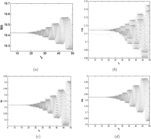This phenomenon can be described in Figure 1. Similarly, we have ${\omega }_{20}=2.6088$, ${\tau }_{20}=17.7622$ for ${\tau }_1=0,{\tau }_2>0$. The numerical simulation is as shown in Figure 2.

Figure 1. The bifurcation diagram with respect to ${\tau }_1$ when ${\tau }_2=0$.

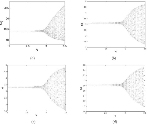
Figure 2. The bifurcation diagram with respect to ${\tau }_2$ when ${\tau }_1=0$.

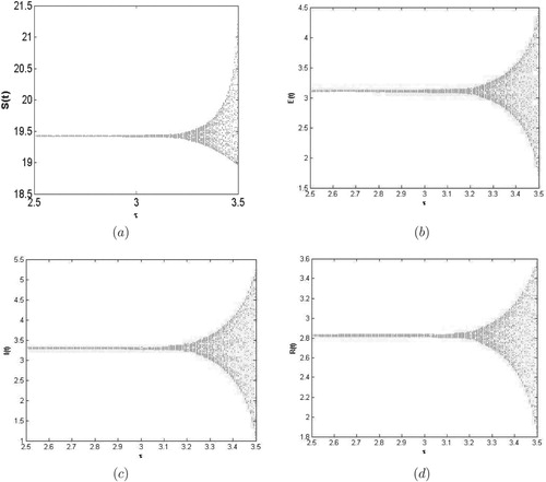
For ${\tau }_1={\tau }_2=\tau >0$, we obtain ${\omega }_0=2.9544$, ${\tau }_0=3.0884$ by some complex computations. As can be seen from the bifurcation diagram with respect to τ in Figure 3, when $\tau <{\tau }_0=3.0884$, $P_{\ast }(19.4224,3.1112,3.3150$, $2.8258)$ is asymptotically stable and a Hopf bifurcation occurs at the critical value of τ. In this case, a family of periodic solutions bifurcate from $P_{\ast }(19.4224,3.1112,3.3150$, $2.8258)$.

Figure 3. The bifurcation diagram with respect to τ when ${\tau }_1={\tau }_2=\tau$.

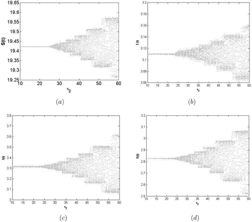
We have ${\omega }_{20}^{\ast }=0.2762$, ${\tau }_{20}^{\ast }=24.8926$ when ${\tau }_1=1.25\in (0,{\tau }_{10})$ and ${\tau }_2>0$ is considered as a bifurcation parameter. The bifurcation diagram with respect to ${\tau }_2$ and ${\tau }_1=1.25\in (0,{\tau }_{10})$ can be shown in Figure 4. In addition, we obtain ${\mu }_2=149.6526>0$, ${\beta }_2=-96.0988<0$ and $T_2=264.0964>0$. Thus, based on the results in Theorem 3.1, we can deduce that the Hopf bifurcation is supercritical, the bifurcating periodic solutions are stable and the period of the bifurcating periodic solutions increase.

Figure 4. The bifurcation diagram with respect to ${\tau }_2$ when ${\tau }_1=1.25\in (0,{\tau }_{10})$ and ${\tau }_2>0$.

5. Conclusions

This paper is concerned with a delayed SEIR epidemic model with saturated incidence and saturated treatment function. The effect of the two delays on the model is investigated and the main results are given in terms of local stability and local Hopf bifurcation. It has been shown that the model is stable when the value of the bifurcation parameter is below the critical value, which means that the disease can be controlled easily. However, when the value of the bifurcation parameter is above the critical value, a Hopf bifurcation will occur. In this condition, the disease is out of control. Accordingly, we should shorten the delays in the model as much as possible so that we can predict and control the disease propagation. For further investigation, the properties of the Hopf bifurcation are studied with the aim of the normal form method and centre manifold theorem. Finally, some numerical simulations are carried out to support our theoretical results.

Acknowledgements

The author is grateful to the editor and the anonymous referees for their valuable comments and suggestions on the paper.

Disclosure statement

The author declares that she has no competing interests.

Additional information

Funding

This work was supported by the University Top-notch Scholarship Program of Anhui Province (gxbjZD49) and Bengbu University National Research Fund Cultivation Project (2017GJPY03).

References

- L. Acedo, G. Gonzlez-Parra and A.J. Arenas, An exact global solution for the classical epidemic model, Nonlinear Anal. RWA 11 (2010), pp. 1819–1825. doi: 10.1016/j.nonrwa.2009.04.007
- C. Bianca, M. Ferrara and L. Gurrini, The Cai model with time delay: Existence of periodic solutions and asymptotic analysis, Appl. Math. Inf. Sci. 7 (2013), pp. 21–27. doi: 10.12785/amis/070103
- C. Bianca and L. Guerrini, Existence of limit cycles in the Solow model with delayed-logistic population growth, Sci. World J. 207806 (2013), pp. 8.
- V. Capasso and G.A. Serio, Generalization of the Kermack–Mckendrick deterministic epidemic model, Math. Biosci. 42 (1978), pp. 41–61. doi: 10.1016/0025-5564(78)90006-8
- F.F. Chen and L. Hong, Stability and Hopf bifurcation analysis of a delayed SIRS epidemic model with nonlinear saturation incidence, J. Dyn. Control 12 (2014), pp. 79–85 (in Chinese).
- Y. Enatsu, E. Messina, Y. Muroya, Y. Nakata, E. Russo and A. Vecchio, Stability analysis of delayed SIR epidemic models with a class of nonlinear incidence rates, Appl. Math. Comput. 218 (2012), pp. 5327–5336.
- B.D. Hassard, N.D. Kazarinoff and Y.H. Wan, Theory and Applications of Hopf Bifurcation, Cambridge University Press, Cambridge, 1981.
- Z.X. Hu, S. Liu and H. Wang, Backward bifurcation of an epidemic model with standard incidence rate and treatment rate, Nonlinear Anal. RWA 9 (2008), pp. 2302–2312. doi: 10.1016/j.nonrwa.2007.08.009
- X.L. Li and J.J. Wei, On the zeros of a fourth degree exponential polynomial with applications to a neural network model with delays, Chaos Solitons Fractals 26 (2005), pp. 519–526. doi: 10.1016/j.chaos.2005.01.019
- W. Ma, M. Song and Y. Takeuchi, Global stability of an SIR epidemic model with time delay, Appl. Math. Lett. 17 (2004), pp. 1141–1145. doi: 10.1016/j.aml.2003.11.005
- Y. Nakata and T. Kuniya, Global dynamics of a class of SEIRS epidemic models in a periodic environment, J. Math. Anal. Appl. 363 (2010), pp. 230–237. doi: 10.1016/j.jmaa.2009.08.027
- J.J. Wang, J.Z. Zhang and Z. Jin, Analysis of an SIR model with bilinear incidence rate, Nonlinear Anal. RWA 11 (2010), pp. 2390–2402. doi: 10.1016/j.nonrwa.2009.07.012
- L.S. Wen and X.F. Yang, Global stability of a delayed SIRS model with temporary immunity, Chaos Solitons Fractals 38 (2008), pp. 221–226. doi: 10.1016/j.chaos.2006.11.010
- R. Xu and Z.E. Ma, Stability of a delayed SIRS epidemic model with a nonlinear incidence rate, Chaos Solitons Fractals 41 (2009), pp. 2319–2325. doi: 10.1016/j.chaos.2008.09.007
- Y.K. Xue and T.T. Li, Stability and Hopf bifurcation for a delayed SIR epidemic model with logistic growth, Abstr. Appl. Anal. 2013 (2013), pp. 1–11.
- H. Yang and J.J. Wei, Stability of SIR epidemic model with a class of nonlinear incidence rates, Appl Math A J Chin. Univ. 29 (2014), pp. 11–16 (in Chinese).
- J.F. Zhang, Bifurcation analysis of a modified Holling–Tanner predator–prey model with time delay, Appl. Math. Model. 36 (2012), pp. 1219–1231. doi: 10.1016/j.apm.2011.07.071
- Y.Y. Zhang and J.W. Jia, Hopf bifurcation of an epidemic model with a nonlinear birth in population and vertical transmission, Appl. Math. Comput. 230 (2014), pp. 164–173. doi: 10.1016/j.camwa.2013.11.007
- J.H. Zhang, J.W Jia and X.Y. Song, Analysis of an SEIR epidemic model with saturated incidence and saturated treatment function, Sci. World J. 2014 (2014), pp. 11. Article ID 910421.
- T.L. Zhang, J.L. Liu and Z.D. Teng, Stability of Hopf bifurcation of a delayed SIRS epidemic model with stage structure, Nonlinear Anal. RWA 11 (2010), pp. 293–306. doi: 10.1016/j.nonrwa.2008.10.059
- Z.Z. Zhang and H.Z. Yang, Hopf bifurcation analysis for a delayed SIRS epidemic model with a nonlinear incidence rate, J. Donghua Univ. (Eng. Ed.) 31 (2014), pp. 201–206.