
 ?Mathematical formulae have been encoded as MathML and are displayed in this HTML version using MathJax in order to improve their display. Uncheck the box to turn MathJax off. This feature requires Javascript. Click on a formula to zoom.
ABSTRACT
This paper proposes a discrete switching predator-prey model with a mate-finding Allee effect, where also switches are guided by Allee effect. One of the strategies analysed is to use a chemical in order to prevent the pest outbreak when the pest population is free of Allee effect. In this paper, we first study analytically the dynamic behaviors of the two subsystems and the equilibria and their stability of the switched system. Then we provide numerical bifurcation analyses for the switched discrete system. These show that the switched discrete system may have very complex dynamics by 2-parameter bifurcation diagrams which divide the space into regions and study equilibria, and 1-dimensional bifurcation diagrams which reveal that the system has periodic, chaotic solutions, period doubling bifurcations and so on. Furthermore, we try to refer the key parameters and initial densities of both populations associated with pest outbreaks and study their biological implications.
1. Introduction
The Allee effect [Citation1, Citation2], which was first described by Allee in the 1930s, has been a relevant topic in ecology but has suffered from widespread confusion since no clear definition had been given before 1999. During this year Stephens et al. [Citation29] defined it as: a positive relation ship between any component of individual fitness and either numbers or density of conspecifics, and suggested that it is important to differentiate between component Allee effects and demographic Allee effects.
The formal definition of these two effects has been described by Fauvergue in 2003 [Citation14]. The former one is a decrease in any component of fitness with decreasing population size or density. Especially, a decrease in the probability of a female mating with decreasing male population is therefore a mate-finding Allee effect. The latter one is a decrease in per capita growth rate with decreasing population size, and it can be divided into a weak and strong demographic Allee effect according to the sign of population growth: the weak effect's growth remains positive even for the smallest populations while the strong effect's growth may become negative when population size decreases below the Allee threshold. Allee effect plays an important role in the conservation of endangered and exploited species, detailed investigations relating Allee effect may be found in the paper [Citation3–5, Citation8–10, Citation13, Citation14, Citation19–23, Citation29, Citation31, Citation32, Citation39].
Meanwhile, it is well known that the outbreak of pests often cause serious ecological and economical problems. In order to control pest more effectively, at the same time, environmental influences and human interventions are taken into account, the Integrated Pest Management (IPM) strategy has been proposed [Citation28, Citation30, Citation35]. One of the important concepts in IPM strategy is the Threshold Policy Control (TPC) [Citation25, Citation26, Citation33, Citation34], which maintains the pests' density below the Economic Injury Level (EIL) [Citation24] by releasing predators and spraying pesticides once the pests' density reaches the Economic Threshold (ET) [Citation6, Citation17], see Figure . The main purpose of IPM is to maintain the density of the pests below the EIL rather than seeking to eradicate them, and the suitable tactic will only be applied as the density of pests reaches the given ET, when it can minimize the damage of insecticides to non-target pests and to preserve the quality of the environment.
Figure 1. EIL: the lowest population density that will cause economic damage. ET: population density at which control measures should be invoked to prevent an increasing pest population from reaching EIL.
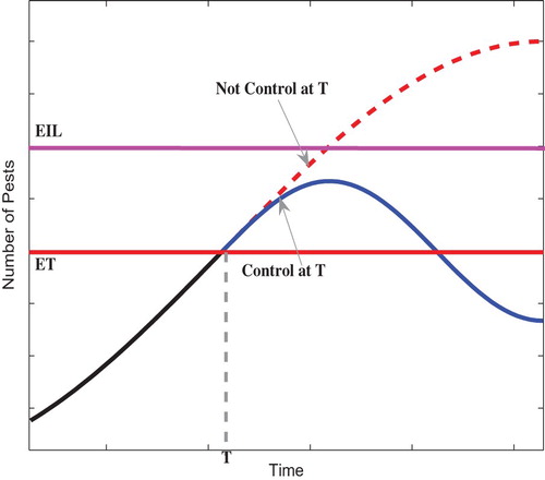
Based on the concept of Allee effect and IPM strategy, we can define the threshold policy control (TPC) related to the IPM and Allee effect in this paper as follows [Citation33, Citation34]: integrated control (spraying pesticides) is suppressed when the pest population abundance is below a previously chosen threshold density ET, i.e. the pest population is subject to a mate-finding Allee effect; above the threshold, integrated control measures are applied. In order to maintain the density of pest population below the EIL, IPM tactics must be applied once its density reaches and exceeds the ET to avoid delay in response to the control measures. Thus, the ET is chosen as the threshold value to guide the switches of the systems in present work.
By employing the above threshold policy control (TPC), a switching system (or non-smooth filippov system) has been proposed and studied in present work. Recently, a non-smooth dynamical theory has been developed to study switchings in science and engineering [Citation12, Citation15], in ecological systems [Citation27, Citation40], and in epidemiological dynamics [Citation37, Citation38, Citation41]. The main goal of this work is to give people a better understanding of a mate-finding Allee effect in a discrete switching predator-prey model. In order to achieve this goal, the effects of switching system on the successful pest control are investigated, as well as the dynamic complexity of proposed switching predator-prey model and their biological implications related to pest control are addressed. The results indicate that a highly Allee effect could decrease the range of the dynamical behaviors of the system, and play a very important role in pest control, initial densities could impact on pest outbreaks. To our knowledge, no work has done for a discrete switching predator-prey model with a mate-finding Allee effect.
The rest of the paper is organized as follows: In the next section, a discrete switching predator-prey model with a mate-finding Allee effect is proposed. The qualitative analysis of two subsystems are given in Section 3. In Section 4, bifurcation analyses including 2-parameter bifurcation and 1-dimensional bifurcation diagrams are studied. In Section 5, we study the importance and relevance of key parameters and initial values of both pest and nature enemy populations in pest outbreaks, analyse switching frequencies through numerical simulations and include some final considerations.
2. Model formulation
In 2011, Wang et al. [Citation39] proposed a discrete ecosystem with a mate-finding Allee effect as follows:
(1)
(1)
The assumptions in model (Equation1(1)
(1) ) are as follows:
and
The term
The term
The mate-finding Allee effect only takes place when the density of the pest population is below the threshold value ET which is the critical point. In case the density is above the threshold value, the mate-finding Allee effect term should be omitted. So model (Equation1(1)
(1) ) can be rewritten as
(2)
(2) Model (Equation2
(2)
(2) ) has been researched by Celik and Duman [Citation5] in 2009, he studied the stability of equilibria.
In order to prevent the outbreak of disaster pests, a chemical control strategy is applied with a proportional killing rate q for pest population only when the density of pest population exceeds the threshold level ET. This yields naturally the following control model with IPM strategy
(3)
(3) Consequently, combining model (Equation3
(3)
(3) ) with IPM when the density of pest population exceeds ET and model (Equation1
(1)
(1) ) without control measures when the density falls below ET, the following switching model included by a mate-finding Allee effect is derived
(4)
(4) Model (Equation4
(4)
(4) ) represents a dynamical system subject to a threshold policy, which is referred to as an on-off control or as a special and simple case of variable structure control in the literatures [Citation33, Citation34].
3. Qualitative analysis for two subsystems
In this section, the existence and stability of positive equilibria of the two subsystems for model (Equation4(4)
(4) ) are investigated, which will be useful for studying the dynamical behaviors of switching model (Equation4
(4)
(4) ). For convenience, we denote
with vector
and
Then model (Equation4
(4)
(4) ) can be rewritten as the following switching system (or filippov system)
(5)
(5) where
From now on, we call switching system (Equation4(4)
(4) ) defined in region
(resp.
) as system
(resp.
).
The following definitions on regular equilibria of switching system [Citation11, Citation16, Citation27, Citation37, Citation38, Citation40], the Lambert W function [Citation7, Citation36] and the switching frequencies are introduced in this section and will be used throughout this paper.
Definition 3.1
A point is called a real equilibrium of switching system (Equation5
(5)
(5) ) if
, or
.
will be denoted by
or
. Analogously, a point
is called a virtual equilibrium if
, or
.
will be denoted by
or
. Both real and virtual equilibria are called regular equilibria.
Definition 3.2
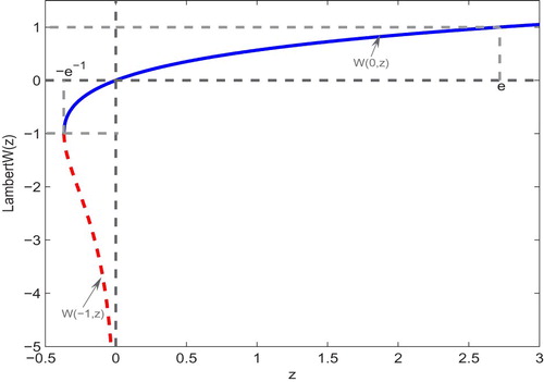
The Lambert W function is a multivalued inverse of the function satisfying
(6)
(6) It follows from (Equation6
(6)
(6) ) that
For simplicity, the inverse function of
on
and
will be denoted by
and
, respectively. Obviously,
and
are the real branches of the Lambert W function. In particular,
is a monotonically increasing function on
, while
is a monotonically decreasing function on
, see Figure for detail.
Figure 2. The two real branches and
of Lambert W function.
Definition 3.3
In switching system (Equation5(5)
(5) ), if
and
(or
and
), then system (Equation5
(5)
(5) ) experiences one time switch and t is called as switch-point. The interval generations between two switch-points is defined as switching frequency.
3.1. Stability of equilibria for system
If , then the qualitative behaviors of system (Equation5
(5)
(5) ) are determined by system
. Obviously, system
has the trivial equilibrium
and the natural-enemy free equilibrium
, which are not stable. Meanwhile, system
has the unique positive equilibrium
which will be shown in the following theorem.
Theorem 3.1
If then system
presents a unique positive equilibrium
which satisfies
Proof.
It follows from subsystem that
should satisfy
For convenience, we denote
Taking derivative of
with respect to x, one yields
Rearranging the above equation we have
(7)
(7) It is easy to see that
and according to Definition 3.2, solving Equation (Equation7
(7)
(7) ) with respect to x, one yields a unique positive root
On the one hand, by a simple calculation, it gives that (i) if
, then
; (ii) if
, then
. Those show that
is the local maximum point of
, and since
, we can apply the monotonicity property of the Lambert W function which yields
thus
.
On the other hand, according to Definition 3.2, it can be shown that , so we have
i.e. the equality
holds true. Thus we can derive that
. Since
satisfies the following properties:
,
as
, it is trivial to see that the point
is a unique extreme point of
and
.
Therefore, combining the following inequalities: with
, it is easy to show that there is always a unique positive root on the interval
provided that
. The proof is completed.
Now we are in a position to investigate the local stability of the unique positive equilibrium of system
.
Theorem 3.2
If the following inequalities
hold, the positive equilibrium point
of system
is asymptotically stable, and
The proof of Theorem 3.2 is similar to that shown in [Citation39] and we omit it.
3.2. Stability of equilibria for system
If , then the qualitative behaviors of system (Equation5
(5)
(5) ) are determined by system
. Obviously, system
has a trivial equilibrium
, which is unstable. In the case in which the following inequality holds:
system
has a unique positive equilibrium
, where
In the following theorem, the local stability of the positive equilibrium point
is proved.
Theorem 3.3
The unique positive equilibrium point of system
is asymptotically stable provided that
(8)
(8) where
(9)
(9)
Proof.
Linearizing system about
, then we can obtain the characteristic equation about the Jacobian Matrix
of system
(10)
(10) The conditions (Equation8
(8)
(8) ) ensure that all the inequalities
hold, that is, the modulus of all roots of Equation (Equation10
(10)
(10) ) are less than 1. By employing the Jury Criteria [Citation18], we can derive that the equilibrium point
of system
is local asymptotically stable. The proof is completed.
4. Complex dynamical behaviors analysis
In this section, we investigate the complex dynamical behaviors of switching system (Equation5(5)
(5) ). Differently from models (Equation1
(1)
(1) ) and (Equation3
(3)
(3) ), the switching system (Equation5
(5)
(5) ) describes the threshold control policy and the mate-finding Allee effect in a much more complex way. The system (Equation5
(5)
(5) ) is a complicated nonlinear dynamical system which is difficult to analyse theoretically so we will focus on the bifurcation phenomena through numerical simulations.
4.1. Equilibria bifurcation for the switching system (eqn5)
According to Definition3.1, the switching system has different types of equilibria [Citation11, Citation16], and these equilibria play a key role in pest control. Especially, Tang et al. [Citation27] studied pest control with economic threshold. It is difficult to find closed forms for all the interior equilibrium of subsystem because of the complexity of Allee effect (the nonlinear term), thus the existence of regular equilibria (real and virtual equilibria) and their coexistence will be given by numerical simulation.
We choose r and ET as bifurcation parameters and fix all others as given in Figure . In our simulations, ET varies from 0.01 to 0.42 and r varies from 0.2 to 0.85, the parameter space is divided into six regions as shown in Figure . In these parameter regions, the existences of regular equilibria depend on the value of r and ET. For example, when the intrinsic growth rate r is relatively small (here ), the space can be divided into two regions: I-1 (yellow) and region I-2 (green). In region I-1 only
exists, while in region I-2 only
exists. However, when the intrinsic growth rate r increases and exceeds a certain threshold value r = 0.28, that is, when
, the results show that the parameter space has been divided into four regions which are region II-1 (red), II-2 (blue), II-3 (cyan), II-4 (magenta). In region II-1,
and
coexist; In region II-2,
and
coexist; In region II-3,
and
coexist; In region II-4,
and
coexist.
Figure 3. Bifurcation diagram for the existence of regular equilibria of system (Equation5(5)
(5) ) with respect to r and ET, parameters are
.
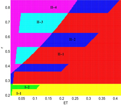
Obviously, a number of bifurcations occur in Figure as the parameters change. One of the main purposes here is to design optimal control strategies to prevent pest outbreaks or keep the density of the pest population below ET. From a mathematical viewpoint, this can be realized if system can stabilize at the desired level through the integration of different control strategies. To realize this purpose, we can choose the desirable threshold level such that all equilibria of subsystem become virtual. Thus, in order to prevent the pest outbreak, parameters r and ET should be carefully chosen to keep the interior equilibria of two subsystems in regions I-1, I-2, II-1 and II-2.
4.2. Bifurcation analysis about sensitive parameters
1-dimensional bifurcation analysis is a traditional approach to gain preliminary insight into the properties of a dynamic system, it provides information about the dependence of the dynamics on a certain parameter space. The analysis is expected to reveal the types of attractors and their changes with parameter variations.
To investigate the complex dynamics that system (Equation5(5)
(5) ) can have, we first choose the intrinsic growth rate r as the bifurcation parameter and fix all other parameters as those in Figure . It follows from Figure that system (Equation5
(5)
(5) ) has more complex and interesting dynamic behaviors. That is, when r increases from 2.18 to 2.7, we can find periodic, chaotic solutions, period doubling, multi-stability, crises and so on. As the parameter r further increases from 2.18 to 2.19, system (Equation5
(5)
(5) ) has a stable solution, see Figure [A] for detail when r = 1.9. When r further increases from 2.19 to 2.2066, system (Equation5
(5)
(5) ) has a periodic solution, see Figure [B] for details. However, a chaotic solution emerges abruptly when r becomes larger and reaches 2.4 or 2.65, see Figures [C,D] for phase plan.
Figure 4. Bifurcation diagram for system (Equation5(5)
(5) ) with respect to r. All other parameters as follows:
and
.
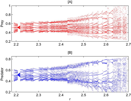
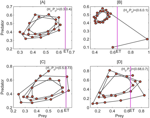
Figure 5. Phase-plan of system (Equation5(5)
(5) ) with different r. [A] r = 2.18; [B] r = 2.213; [C] r = 2.4; [D] r = 2.65. The other parameters are identical to those in Figure .
![Figure 5. Phase-plan of system (Equation5(5) Z˙(t)={FS1(Z),Z∈S1,FS2(Z),Z∈S2,(5) ) with different r. [A] r = 2.18; [B] r = 2.213; [C] r = 2.4; [D] r = 2.65. The other parameters are identical to those in Figure 4.](/cms/asset/070dbf1d-0c34-44ee-90e6-19ccad3e9887/tjbd_a_1682200_f0005_oc.jpg)
Furthermore, the complex and interesting dynamic behaviors of system (Equation5(5)
(5) ) can also be shown respectively through Figures and , where we choose the killing rate q and the Allee effect constant θ as the bifurcation parameter. Comparing Figure [A] with Figures [B] or [C], the chaos may be removed if the pests are subject to a highly effective Allee effect. Meanwhile, the local stability of the equilibrium point increases with a highly effective Allee effect, see Figures [B,C] for detail. Furthermore, Figure [A] is proof of the fact that dynamical behaviors are very complicated since there may be several hidden factors that can adversely affect our control strategy. However, if we take some control measures to reduce the growth rate of pests, the dynamics of model (Equation5
(5)
(5) ) will become more clear as shown in Figure [B], and this will help to prevent pest outbreaks. Therefore, Figures and indicate that a highly effective Allee effect could decrease the complexity of the dynamical behaviors of the system and play a very important role in pest control.
Figure 6. Bifurcation diagram for system (Equation5(5)
(5) ) with respect to q. All other parameters as follows:
, and [A]
; [B]
; [C]
.
![Figure 6. Bifurcation diagram for system (Equation5(5) Z˙(t)={FS1(Z),Z∈S1,FS2(Z),Z∈S2,(5) ) with respect to q. All other parameters as follows: a=1.68,ET=0.72,r=2.58,(H0,P0)=(0.1,0.1), and [A] θ=9.5; [B] θ=5; [C] θ=1.](/cms/asset/a7fd62d6-4ced-4e6a-a23b-2bd70bb84742/tjbd_a_1682200_f0006_oc.jpg)
Figure 7. Bifurcation diagram for system (Equation5(5)
(5) ) with respect to θ. All other parameters as follows:
, and [A] r = 2.13; [B] r = 2.
![Figure 7. Bifurcation diagram for system (Equation5(5) Z˙(t)={FS1(Z),Z∈S1,FS2(Z),Z∈S2,(5) ) with respect to θ. All other parameters as follows: a=2,q=0.8,ET=0.8,r=2.29,(H0,P0)=(0.3,0.2), and [A] r = 2.13; [B] r = 2.](/cms/asset/03d0b846-e5f8-444a-8608-b85eb57fe996/tjbd_a_1682200_f0007_oc.jpg)
5. Initial sensitivities and switching effects
It is well known that the dynamics can change given different initial densities of both pest and natural-enemy populations. This section focuses on how the initial densities of pest and natural enemy populations affect the control strategies. In addition, we will discuss the effects of key parameters on the switching frequencies of system (Equation5(5)
(5) ).
5.1. Initial sensitivities
Firstly, in order to investigate the interaction between the initial densities of populations and pest control, Figure illustrates the switch effects of initial densities on IPM strategy. In Figure [A] the initial densities are and the simulation result indicates that the pest density never reaches the given ET = 0.65, which shows the solution initiating from
is free from IPM measures. If we set the initial densities as
or
, the results indicate that the switching system (Equation5
(5)
(5) ) is free from IPM control after 1 or 2 applications of the IPM strategies, see Figures [B] and [C]. However, when the initial densities are
, in order to control the pest population below ET, it is necessary to apply IPM measures several times, see Figure [D] for detail.
Figure 8. Switching effect of system (Equation5(5)
(5) ) under different initial densities. Parameters are
.
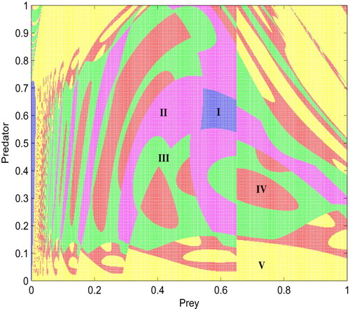
In addition, we discuss the interaction between initial densities and pest outbreak studying the phase-plane in Figure . This plot is separated in five different regions denoted by I (blue), II (magenta), III (green), IV (red), V (yellow). In region I, the pest population never outbreaks and is always stabilized in subsystem ; In regions II, III and IV, pest density is below the given threshold ET provided that IPM control measures are applied 1, 2 and 3 times, respectively; In region V, the switching system (Equation5
(5)
(5) ) could experience the pest control intervention several times. To sum up, these results indicate that different initial densities may result in different final states of the pest.
Figure 9. Pest outbreak frequency depends on initial density of system (Equation5
(5)
(5) ). The parameters are fixed as
.
Furthermore, the initial densities could also affect the multiple attractors. According to the bifurcation analyses shown in Figures , and , the multiple attractors can coexist for a wide range of parameters. To confirm this and discuss their biological implications, we fix all parameters as those in Figure and choose different initial densities. In particular, two different pest-outbreak attractors coexist at , as shown in Figure , which display different amplitudes and frequencies. If we let the initial values be
, then the solution of system (Equation5
(5)
(5) ) approaches the periodic attractor shown in Figure [A]. On the other hand, we choose the initial value
, the outbreak patterns for pest population become quite complex and a new, unexpected attractor can be seen, as shown in Figure [B].
Figure 10. The coexisting attractors of system (Equation5(5)
(5) ) with different initial values. Parameters are
, and [A]
; [B]
.
![Figure 10. The coexisting attractors of system (Equation5(5) Z˙(t)={FS1(Z),Z∈S1,FS2(Z),Z∈S2,(5) ) with different initial values. Parameters are a=2,θ=4,q=0.05,ET=0.45,r=2.3, and [A] (H0,P0)=(0.6,0.4); [B] (H0,P0)=(0.1,0.1).](/cms/asset/faff0f16-3dee-4174-bfaa-3a83b963ec38/tjbd_a_1682200_f0010_oc.jpg)
In order to better analyse the initial sensitivities in the examples of Figure , in order to illustrate the corresponding initial sensitivities more specifically, basins of attraction with respect to two different pest-outbreak are shown in Figure where the white and black points are attracted to the attractor shown in Figures [A,B]. We can also see that the line ET = 0.45 separates the attraction regions into two parts. The final stable states of pest and natural-enemy depend on their initial densities, and those results are confirmed by the basins of attraction of initial densities. From a pest control view point, the integrated control strategies may strictly depend on the initial densities of both populations since different attractors have different outbreak amplitudes and frequencies.
Figure 11. Basin of attraction of two attractors shown in Fig. with and
. The white and black points are attracted to the attractors shown in Figure from left to right.
![Figure 11. Basin of attraction of two attractors shown in Fig. 10 with H∈[0.3,0.67] and P∈[0.2,0.8]. The white and black points are attracted to the attractors shown in Figure 10 from left to right.](/cms/asset/f6e3ae38-b57b-4045-8477-90d2df92dbd0/tjbd_a_1682200_f0011_ob.jpg)
Therefore, numerical simulations indicate that the successful biological control depends on the initial densities of both pest and natural-enemy populations. This is because these initial densities can affect the outcome of pest populations and can help us design proper control strategies.
5.2. Switching frequency
In this subsection, the effects of the key parameters on the switching frequencies of system (Equation5(5)
(5) ) are investigated.
Firstly, in order to understand how the different intrinsic growth rates of pest population affect pest outbreak, the switching system (Equation5(5)
(5) ) is rewritten as
(11)
(11) where
is random perturbation of q, u is uniformly distributed variable on
and
represents the intensity of noise. What we want to address in this section is how the intensity of noise affects the pest-outbreak amplitudes and whether the stable attractors switch from one attractor to another or not.
To show this, we fix and the other parameters as in Figure . If we randomly perturb the releasing constant r every 90 generations with an intensity
, then the attractors switch-like behavior occurs. In Figure [A], within the first 90 generations, the first stable attractor has a really small amplitude and the pests' densities are below ET. Once the random perturbation occurs at the
generation, system (Equation11
(11)
(11) ) quickly switches to a stable pest-outbreak attractor with medium amplitude. At the
generation, on the other hand the third pest-outbreak attractor can switch to the chaos attractor with large amplitude and in this case it is much more difficult to control the pest population.
Figure 12. Attractors' switch-like behavior of system (Equation5(5)
(5) ) with
has random perturbation as each 90 generations. Parameters are:
and
.
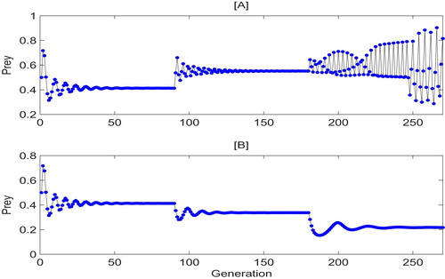
Interesting to notice is also the fact that system (Equation11(11)
(11) ) can yield completely different dynamics due to the randomness of the perturbation as it can be seen in Figure [B]. The amplitudes of of these three stable attractors decrease gradually and below ET = 0.5, i.e. the pest population is under control as desired.
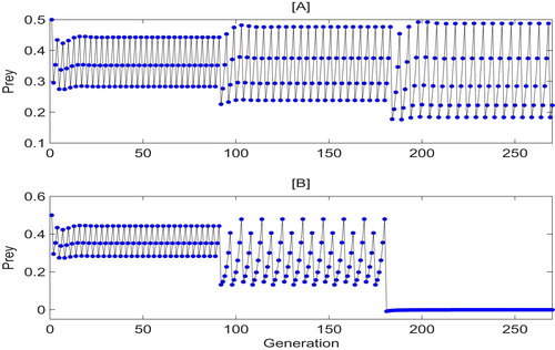
Analogously, to address the effects of different killing rates on a switch-like behavior, we rewrite switching system (Equation5(5)
(5) ) as
(12)
(12) where
is a random perturbation of q,
represents the intensity of noise. By numerical simulations, we can see from Figure that a similar switch-like behavior can occur once
is randomly perturbed at every 90 generations with relatively large intensity (i.e.
). Both Figures and indicate that one solution can switch to another attractor with small amplitude at a random time when a small changes are introduced the parameters. That is, the perturbation of parameter can affect the pest outbreak and bring some challenges for pest control, it is essential to consider this factor as we design control strategies and make management decisions.
Figure 13. Attractors' switch-like behavior of system (Equation5(5)
(5) ) with
which random perturbation every 90 generations. Parameters are:
and
.
The perturbation of the parameter can bring some challenges for pest control
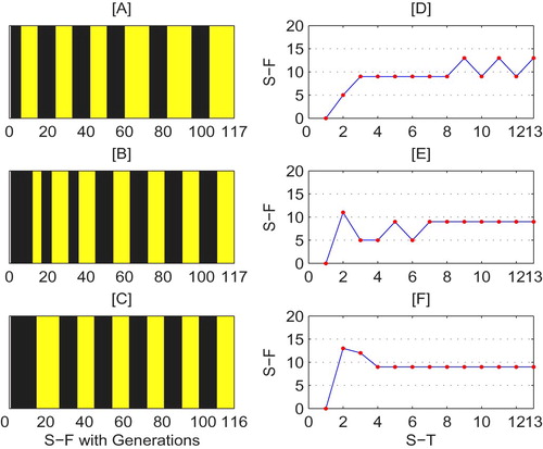
Furthermore, we investigate the effects of initial densities on switching frequencies. Figure [A–C] shows the switching frequencies of system (Equation5(5)
(5) ) with different initial densities, while Figure [D–F] show the relationship between the switching times and frequencies corresponding to Figure [A–C], respectively. In particular, the switching frequencies of Figure [E,F] are stable at 9, while the switching frequencies of Figure [D] fluctuate between 9 and 13. Moreover, it can be seen that the switching frequencies of Figure [F] converge three times quicker than Figure [E], since the system experiences 3 and 6 times switching in Figure [F] and [E], respectively. If the switchings occur frequently, then the control measures must be applied more times and this would mean that pesticide applications should be utilized frequently. Unfortunately, this is not cost effective and may lead to adverse effects such as environmental pollution problems. Therefore, the state of the switching frequencies with respect to the switching times depends on the initial values, which can helps us to design suitable control measures for pest control.
Figure 14. Switching frequency (S-F) and switching time (S-T) of system (Equation5(5)
(5) ). Parameters are
. The initial densities from top to bottom are
and
.
6. Discussion and biological conclusions
In this contribution, we have deduced a discrete switching predator-prey model with a mate-finding Allee effect where switch strategies and control measures are guided by an economic threshold. The overall objective of this paper is to investigate the long-term dynamic behavior of the discrete switching predator-prey model (Equation5(5)
(5) ). In order to work towards this goal, many dynamical system elements have been analyzed in this paper including 2-parameter bifurcation diagrams, 1-dimensional bifurcation, initial sensitivity, multiple attractors and switching frequency. Our finding demonstrates that a highly effective Allee effect could decrease the complexity of the dynamical behaviors of the system and plays a very important role in pest control. In particular, the initial densities could greatly impact on pest outbreaks and IPM measures.
For these reasons, the existence and stability of equilibria of subsystems of model (Equation5(5)
(5) ) have to be investigated. There may be some hidden factors that change dramatically the dynamical behavior of the switching system which increases in complexity making pest control decisions more challenging. To show this, we analyse the possible bifurcation behaviors that model (Equation5
(5)
(5) ) can exhibit, as can be seen in Figures , , and . In Figure , the 2-parameter bifurcation diagrams reveal that the regions contain both regular and virtual equilibria. From a pest control view point, it is necessary to design the desirable threshold level ET or appropriate control strategies such that all equilibria of subsystems
and
become virtual. That is, in order to prevent pest outbreak, parameters r and ET should be carefully chosen to keep the internal equilibria of two subsystems
and
in region II-2 in Figure .
On the other hand, the 1-dimensional bifurcation diagrams (see Figures , and for details) which derive from the switching system (Equation5(5)
(5) ) presents various dynamical behaviors such as periodic and chaotic solutions, multi-stability, periodic window, crises, period doubling and halving bifurcations etc. According to bifurcation diagrams, we can find that the routes to chaos are very complicated, which indicates that there are several hidden factors that can adversely affect our control strategy. The increasing number of potential complexities predicted by the theory is a major challenge for pest control in practice. However, the results in Figure indicate that the chaoticity may be removed if the pests are subject to a highly effective Allee effect, and the local stability of the equilibrium increases with a highly effective Allee effect since it could decrease the complexity of the dynamical behaviors of the s, and is a key factor in pest control.
Furthermore, the correlations between initial densities and pest control are investigated. It is shown in this paper that the initial densities of pest and natural-enemy populations can affect the outcome of classical biological control, and the final stable states of both populations depend on their initial densities, see Figures , , and . These results are further confirmed by the switching frequencies since the eventually state of the switching frequencies with respect to the switching times depends on the initial values shown in Figure .
In our study, we have investigated the dynamical behavior of a discrete switching predator-prey model with a mate-finding Allee effect. To link the costs of developing and implementing controls to population dynamic modeling, it is necessary to consider resource limitation factors such as limited capacity for pesticides, costs and since such nonlinear factors can affect the outcome of pest control. These topics will be considered in further work in the future.
Acknowledgments
We would like to thank Dr. Marco Tosato of York University for helping us revise English that greatly improved the presentation of this paper. In addition, the authors wish to thank the editor and the reviewers for their valuable comments and suggestions that greatly improved the presentation of this work.
Disclosure statement
No potential conflict of interest was reported by the author.
ORCID
Wenjie Qin http://orcid.org/0000-0002-5635-1534
Additional information
Funding
Related Research Data
References
- W.C. Allee, A. Aggregations: A Study in General Sociology, Chicago, 1931.
- W.C. Allee, O. Park, A.E. Emerson, Principles of Animal Ecology, WB Saundere, Philadelphia, 1949.
- L. Assas, B. Dennis, S. Elaydi, E. Kwessi and G. Livadiotis, Stochastic modified Beverton-Holt model with Allee effect II: the Cushing-Henson conjecture, J. Differ. Equ. Appl. 22 (2016), pp. 164–176. doi: 10.1080/10236198.2015.1075521
- D.S. Boukal and L. Berec, Single-species models of the Allee effect: extinction boundaries, sex ratios and mate encounters, J. Theor. Biol. 218 (2002), pp. 375–394. doi: 10.1006/jtbi.2002.3084
- C. Celik and O. Duman, Allee effect in a discrete-time predator-prey system, Chaos Solitons Fractals,40 (2009), pp. 1956–1962. doi: 10.1016/j.chaos.2007.09.077
- H.C. Chiang, General model of the economic threshold level of pest populations, Plant Protect. Bull (1979).
- R.M. Corless, G.H. Gonnet, D.E.G. Hare and D.J. Jeffrey, On the Lambert W function, Adv. Comput. Math. 5 (1996), pp. 329–359. doi: 10.1007/BF02124750
- M.I.S. Costa and L. dos Anjos, Multiple hydra effect in a predator-prey model with Allee effect and mutual interference in the predator, Ecol. Modell. 373 (2018), pp. 22–24. doi: 10.1016/j.ecolmodel.2018.02.005
- F. Courchamp, T. Clutton-Brock and B. Grenfell, Inverse density dependence and the Allee effect, Trends Ecol. Evol. 14 (1999), pp. 405–410. doi: 10.1016/S0169-5347(99)01683-3
- B. Dennis, Allee effects: population growth, critical density, and the chance of extinction, Nat. Resour. Model. 3 (1989), pp. 481–538. doi: 10.1111/j.1939-7445.1989.tb00119.x
- M. di Bernardo, C.J. Budd, A.R. Champneys, P. Kowalczyk, A.B. Nordmark, G.O. Tost and P.T. Piiroinen, Bifurcations in nonsmooth dynamical systems, SIAM Rev. 50 (2008), pp. 629–701. doi: 10.1137/050625060
- S.H. Doole and S.J. Hogan, A piecewise linear suspension bridge model: nonlinear dynamics and orbit continuation, Dynam. Stability Syst. 11 (1996), pp. 19–47. doi: 10.1080/02681119608806215
- S. Elaydi, E Kwessi and G. Livadiotis, Hierarchical competition models with the Allee effect III: multispecies, J. Biol. Dyn. 12 (2018), pp. 271–287. doi: 10.1080/17513758.2018.1439537
- X. Fauvergue, A review of mate-finding Allee effects in insects: from individual behavior to population management, Entomol. Exp. Appl. 146 (2013), pp. 79–92. doi: 10.1111/eea.12021
- M. Guardia, S.J. Hogan and T.M. Seara, An analytical approach to codimension-2 sliding bifurcations in the dry-friction oscillator, SIAM J. Appl. Dyn. Syst. 9 (2010), pp. 769–798. doi: 10.1137/090766826
- M. Guardia, T.M. Seara and M.A. Teixeira, Generic bifurcations of low codimension of planar Filippov systems, J. Differ. Equ. 250 (2011), pp. 1967–2023. doi: 10.1016/j.jde.2010.11.016
- J.C. Headley, Defining the economic threshold, in Pest Control Strategies for the Future, National Academy of Sciences, Washington, 1972, pp. 100–108.
- E.I. Jury, Inners and Stability of Dynamic Systems, Wiley, 1974.
- R.R.B. Kaul, A.M. Kramer, F.C. Dobbs and J.M. Drake, Experimental demonstration of an Allee effect in microbial populations, Biol. Lett. 12 (2016), pp. 20160070. doi: 10.1098/rsbl.2016.0070
- H. Kokko and W.J. Sutherland, Ecological traps in changing environments: ecological and evolutionary consequences of a behaviourally mediated Allee effect, Evol. Ecol. Res. 3 (2001), pp. 603–610.
- M. Kuussaari, I. Saccheri, M. Camara and I. Hanski, Allee effect and population dynamics in the Glanville fritillary butterfly, Oikos 82 (1998), pp. 384–392. doi: 10.2307/3546980
- M.A. McCarthy, The Allee effect, finding mates and theoretical models, Ecol. Modell. 103 (1997), pp. 99–102. doi: 10.1016/S0304-3800(97)00104-X
- N. Min and M.X. Wang, Dynamics of a diffusive prey-predator system with strong Allee effect growth rate and a protection zone for the prey, Discrete Contin. Dyn. Syst. Ser. B 23 (2018), pp. 995–1004.
- L.P. Pedigo, S.H. Hutchins and L.G. Higley, Economic injury levels in theory and practice, Annu. Rev. Entomol. 31 (1986), pp. 341–368. doi: 10.1146/annurev.en.31.010186.002013
- W.J. Qin, X.W. Tan, M. Tosato and X.Z. Liu, Threshold control strategy for a non-smooth Filippov ecosystem with group defense, Appl. Math. Comput 362 (2019), pp. 124532. doi:10.1016/j.amc.2019.06.046
- W.J. Qin, X.W. Tan, X.T. Shi, J.H. Chen and X.Z. Liu Qin, Dynamics and bifurcation analysis of a Filippov predator-prey ecosystem in a seasonally fluctuating environment, Internat. J. Bifur. Chaos Appl. Sci. Engrg 29(2) (2019), pp. 1950020. doi:10.1142/S0218127419500202
- S.Y. Tang, J.H. Liang, Y.N. Xiao and R.A. Cheke, Sliding bifurcation of fillippov two stage pest control bodels with economic thresholds, SIAM J. Appl. Math. 72 (2012), pp. 1061–1080. doi: 10.1137/110847020
- J.A. Stenberg, A conceptual framework for integrated pest management, Trends Plant Sci. 22 (2017), pp. 759–769. doi: 10.1016/j.tplants.2017.06.010
- P.A. Stephens, W.J. Sutherland and R.P. Freckleton, What is the Allee effect? Oikos 87 (1999), pp. 185–190. doi: 10.2307/3547011
- V. Stern, R. Smith, R. Van den Bosch and K. Hagen, The integrated control concept, Hilgardia, 29 (1959), pp. 81–101. doi: 10.3733/hilg.v29n02p081
- A.W. Stoner and M. Ray-Culp, Evidence for Allee effects in an over-harvested marine gastropod: density-dependent mating and egg production, Mar. Ecol. Prog. Ser. 202 (2000), pp. 297–302. doi: 10.3354/meps202297
- G.Q. Sun, Mathematical modeling of population dynamics with Allee effect, Nonlinear Dyn. 85 (2016), pp. 1–12. doi: 10.1007/s11071-016-2671-y
- V.I. Utkin, Sliding Modes and Their Applications in Variable Structure Systems, Mir Publishers, 1978.
- V.I. Utkin, Sliding Modes in Control and Optimization, Springer-Verlag, 1992.
- R. Van den Bosch, The Pesticide Conspiracy, University of California Press, 1989.
- J. Waldvogel, The period in the Volterra-Lotka predator-prey modle, SIAM J. Numer. Anal. 20 (1983), pp. 1264–1272. doi: 10.1137/0720098
- A.L. Wang, Y.N. Xiao and R.A Cheke, Global dynamics of a piece-wise epidemic model with switching vaccination strategy, Discrete Contin. Dyn. Syst. Ser. B 19 (2014), pp. 2915–2940. doi: 10.3934/dcdsb.2014.19.2915
- A.L. Wang, Y.N. Xiao and H.P. Zhu, Dynamics of a Filippov epidemic model with limited hospital beds, Math. Biosci. Eng. 15 (2018), pp. 739–764. doi: 10.3934/mbe.2018033
- W.X. Wang, Y.B. Zhang and C.Z. Liu, Analysis of a discrete-time predator-prey system with Allee effect, Ecol. Complex. 8 (2011), pp. 81–85. doi: 10.1016/j.ecocom.2010.04.005
- C.C. Xiang, Z.Y. Xiang, S.Y. Tang and J.H. Wu, Discrete switching host-parasitoid models with integrated pest control, Internat. J. Bifur. Chaos Appl. Sci. Eng. 24 (2014), pp. 1450114.
- Y.N. Xiao, X.X. Xu and S.Y. Tang, Sliding mode control of outbreaks of emerging infectious diseases, Bull. Math. Biol. 74 (2012), pp. 2403–2422. doi: 10.1007/s11538-012-9758-5