Stochastic optimal switching model for migrating population dynamics

Abstract

An optimal switching control formalism combined with the stochastic dynamic programming is, for the first time, applied to modelling life cycle of migrating population dynamics with non-overlapping generations. The migration behaviour between habitats is efficiently described as impulsive switching based on stochastic differential equations, which is a new standpoint for modelling the biological phenomenon. The population dynamics is assumed to occur so that the reproductive success is maximized under an expectation. Finding the optimal migration strategy ultimately reduces to solving an optimality equation of the quasi-variational type. We show an effective linkage between our optimality equation and the basic reproduction number. Our model is applied to numerical computation of optimal migration strategy and basic reproduction number of an amphidromous fish Plecoglossus altivelis altivelis in Japan as a target species.

KEYWORDS:

• Stochastic dynamic programming
• fish migration
• Hamilton-Jacobi-Bellman equation
• basic reproduction number
• Plecoglossus altivelis altivelis

Mathematics Subject Classifications:

• 60j60
• 90c39
• 92b05
• 93c30

1. Introduction

Migration of biological organisms is a main driving factor of ecosystems [1,2] as well as a core of many human activities like fisheries [3,4] and agriculture [5,6]. Understanding of interactions between migrating biological organisms and environmental development by human, such as existence of dams and weirs in rivers as migration routes of fish species [7,8], has long been an important topic. Population dynamics of biological organisms can be described with individual-based models based on agents [9,10], spatially heterogeneous models based on partial differential equations (PDEs) [11,12], or simpler spatially-lumped models based on differential or difference equations [13,14].

Optimization models are one of the most standard mathematical models for analysing not only specific parts of life histories such as swimming between habitats [15,16] and foraging in territories [17,18] but also entire life histories and life cycles [19,20]. Stochastic dynamic programming (SDP), also called stochastic optimal control or stochastic optimization, has been an effective tool for modelling population dynamics in natural environment [21,22]. In general, an SDP problem is a maximization, minimization, or a saddle-point problem of an objective function subject to system dynamics to be optimized. In an engineering SDP problem, the decision-maker is human as an inspector of a system as widely seen in problems of manufacturing [23,24], economics [25,26], insurance [27,28], resource management [29,30], ecological management [31,32], and environmental management [33,34]. On the other hand, the decision-maker in a problem of population dynamics is the population themselves [21,22]. This is a significant theoretical difference between problems of engineering and those of population dynamics. Nevertheless, we can apply mathematical tools and techniques established in the engineering research areas to analysis of population dynamics.

Application examples of the SDP to population dynamics are diverse [35]. McHuron et al. [36] applied an SDP model to life cycles of mammals and discussed impacts of stochastic disturbance on the fecundity. Brodin et al. [37] analysed temperature-adaptive behaviour of small birds during winter using an SDP model. An SDP model was employed in analysis of adaptive life-history evolution of butterfly in seasonal environment [38]. Frame and Mills [39] discussed condition-dependent mate choice with an SDP model under the assumption that a female choose mates so that a fitness is maximized. Griffen [40] explained the reason of a reproductive skipping behaviour of an elephant seal using an SDP model and demonstrated importance of foraging behaviour in assessing the phenomenon. Route choice problems of avian migrants have been described with SDP models [41]. Evolution of optimal gut size of birds has been analysed in Ez-zizi et al. [42] based on a time-periodic SDP model. A unified SDP-based numerical tool for modelling animal life histories under temporally cyclic environment has been developed in Schaefer et al. [43]. Satterthwaite et al. [44] developed an SDP model for understanding linkages between migration timing of anadromous salmonids and multiple environmental factors.

From a modern mathematical viewpoint, especially models for continuous-time biological and ecological dynamics, solving an SDP problem ultimately reduces to finding a solution to the corresponding optimality equation often called a Hamilton-Jacobi-Bellman (HJB) equation. HJB equations are often formulated as degenerate elliptic or parabolic partial differential equations [45,46]. In the simplest case where the dynamics is linearized and/or the objective function has a specific form, the corresponding HJB equation is solved analytically [31,47,48]. If the HJB equation to be considered is not analytically solvable, then a numerical approximation method can be applied to dealing with the equation. Versatile numerical methods, such as finite difference methods [49,50], finite element methods [51,52], and Fourier discretization methods [53,54] have been applied to HJB and related equations.

Conventional models of the SDP type sometimes have many variables in return for versatility and are not always easy to analyse in detail. On the other hand, models based on HJB and related equations are more efficient and have been effectively applied to migrating population dynamics especially those occurring in water bodies, like diel fish migration [55], diel migration driven by predator-prey interactions [56], and seasonal fish migration [57,58]. Models based on HJB equations can potentially serve as efficient mathematical tools for analysing life cycle of species to which conventional optimization models have been applied [59,60]. In addition, considering the population dynamics from the viewpoint of HJB formalism would provide a new theoretical linkage between them; an example is presented in this paper. However, such an approach has not been addressed so far to the best of the authors’ knowledge, motivating an application of an HJB formalism to migrating population dynamics.

The objectives and contributions of this paper are to formulate and analyse an SDP model for describing an annual life cycle of migrating single fish species with no overlapping generations, with a particular emphasis on migrating fish having one-year life cycles. From the conventional population dynamics modelling viewpoint, migration dynamics of population among habitats is described with state switching where the migration occurs following certain a probabilistic rule in an open-loop manner [61–63]. On the other hand, in this paper, the dynamics is efficiently described in the framework of a stochastic optimal switching where the decision-maker is the population who decides the timing of migration. The optimal switching (Chapter 5 of Pham [46]) is a concept of stochastic control where the decision-maker controls discrete state variables in a closed-loop and thus state-dependent manner. Szabó et al. [64] utilized a stochastic optimal switching model for describing trading problems in finance. Some models are exactly-solvable and their solution structures have been analysed in detail [65,66]. El Asri and Mazid [67] analysed well-posedness of stochastic differential games between two players both having switching controls. The optimal switching is a potential candidate of migration dynamics between habitats in a feed-back, state-dependent manner that is usual in animal behaviour [35]. However, application of the optimal switching formalism to life cycle modelling of migrating population dynamics has not been addressed so far despite its potential applicability.

In our model, the population dynamics are described with stochastic differential equations (SDEs) [45]. We show that a life cycle of single species, which involves growth, reproduction, and migration of population, can be reasonably described with the stochastic optimal switching, unifying the previous models for a migration event as only a part of life history [57,58]. We demonstrate that finding the optimal migration strategy with the present model reduces to solving an HJB equation, the optimality equation, of the quasi-variational form. The equation can be simplified based on certain assumptions of the coefficients. We show a linkage between the optimality equation and the basic reproduction number [68], which is a central concept to quantify reproduction success.

The model is finally applied to numerical computation of the optimal migration strategy and the basic reproduction number of an amphidromous fish Plecoglossus altivelis altivelis (hereafter referred to as P. altivelis) in Japan. This fish is one of the most commercially and ecologically important fishery resources in the freshwater environment in the country [69,70]. In general, the fish has a unique one-year life history seasonally migrating between the sea and a river. Adult fishes grow up in mid-stream of a river during spring to coming summer by feeding rock-attached algae like diatoms, and migrating together toward the downstream river reach in the coming autumn to spawn. After that the adult fishes die, hatched larvae drift toward the sea. The larvae grow up by feeding mainly on plankton in the sea until coming spring, at which mass migrations of the fish population from the sea to rivers occur. There exist several experimental and field findings on the ecology of the fish [69,71–73]; however, much less attention has been made on modelling the entire life history of the fish. We hope that our methodology in the flavour of operations research, which is hence slightly different from the conventional ones, may open the door toward new mathematical modelling of animal population dynamics.

The rest of this paper is organized as follows. Section 2 presents our mathematical model. Mathematical analysis results on the model are also presented in Section 2. Section 3 applies the model to P. altivelis with a numerical method. Section 4 presents summary and future perspectives of our research. Technical proofs of propositions in the main text are placed in Appendix A.

2. Mathematical modelling

The population dynamics model and objective function to be optimized are formulated, and the optimality equation that governs the optimal migration strategy is derived. The basic reproduction number associated with the present model is then formulated based on the value function.

2.1. Basic problem setting

The present model describes a life cycle (growth, migration, and reproduction) of a population with non-overlapping generations. Amphidromous fishes like P. altivelis in Japan having a one-year life history [69,70] are examples to which the model potentially applies. Our model puts an emphasis on theoretical simplicity, so that it is a candidate of minimal models for describing the population dynamics. We assume that the population seasonally migrates between the two habitats $H_0$ and $H_1$. Figure 1 is a conceptual diagram of the population dynamics considered in this paper. Each migration event is assumed to occur within a much shorter time-scale than that of the whole life history [57,58] and is therefore considered to be impulsive. Partial migration that only a part of population migrates [74] is not considered in this paper. We assume that the population reproduces the next generation during the migration from the habitat $H_1$ toward $H_0$. This kind of spawning behaviour is seen in migratory fish species having one-year life histories like P. altivelis [69], Salangichthys microdon [75], and Hypomesus nipponensis [76]. In the present mathematical framework, the spawning field, which is assumed to be placed between the habitats $H_1$ and $H_0$, is not explicitly considered but is effectively lumped into the corresponding migration event description. The generation change is described as an impulsive total population change. This formulation harmonizes with the present SDP modelling based on the optimal switching.

Figure 1. Conceptual diagram of the population dynamics. The time is represented in the sense of mod $T$.

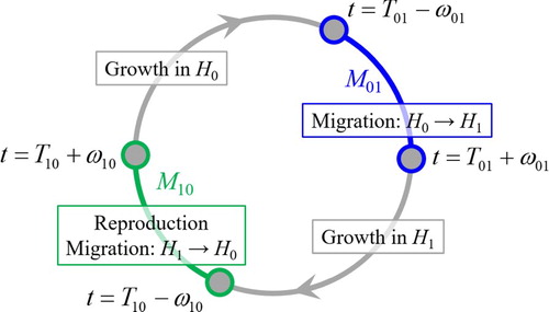
The time is denoted as $t$. The initial time is set as $t=0$. The length of the nominal life cycle is denoted as $T>0$. The kth period, which would be some year in application, is denoted as $L^{\left(k\right)}:\left[\left(k-1\right)T,kT\right)$ $\left(k\in \mathbb{N}\right)$. Assume that the population migrates between the two habitats $H_0$ and $H_1$ in each $L^{\left(k\right)}$ with a manner such that the migration event from $H_0$ to $H_1$ and that from $H_1$ to $H_0$ occur one by one times in this order. Without loss of generality, we set that the population is in $H_0$ at $t=0$. The migration period from $H_0$ to $H_1$ and that from $H_1$ to $H_0$ during $L^{\left(k\right)}$ are expressed with the super-script $\left(k\right)$ as $M_{01}^{\left(k\right)}$ and $M_{10}^{\left(k\right)}$, respectively. They are set as $M_{01}^{\left(k\right)}:\left[T_{01}-{\omega }_{01},T_{01}+{\omega }_{01}\right]$ $\left(modT\right)$ and $M_{10}^{\left(k\right)}:\left[T_{10}-{\omega }_{10},T_{10}+{\omega }_{10}\right]$ $\left(modT\right)$, respectively, where $0<T_{01},T_{10},{\omega }_{01},{\omega }_{10}<T$ are constants. Assuming that these periods do not overlap and that $M_{10}^{\left(k\right)},M_{10}^{\left(k\right)}\subset L^{\left(k\right)}$, we obtain the constraints on the parameters as $0<T_{01}-{\omega }_{01}$, $T_{10}+{\omega }_{10}<T$, and $T_{01}+{\omega }_{01}+{\omega }_{10}<T_{10}$. They hold if ${\omega }_{01}$ and ${\omega }_{10}$ are small and $T_{01}<T_{10}$. Set $T_{01}^{\left(k\right),\pm }=kT+T_{01}\pm {\omega }_{01}$ and $T_{10}^{\left(k\right),\pm }=kT+T_{10}\pm {\omega }_{10}$, meaning that $M_{01}^{\left(k\right)}:\left[T_{01}^{\left(k\right),-},T_{01}^{\left(k\right),+}\right]$ and $M_{10}^{\left(k\right)}:\left[T_{10}^{\left(k\right),-},T_{10}^{\left(k\right),+}\right]$.

The population can migrate from $H_0$ to $H_1$ only in $M_{01}^{\left(k\right)}$, and from $H_1$ to $H_0$ only in $M_{10}^{\left(k\right)}$. We assume that the population does not migrate between the habitats in the other periods, as assumed in life cycle models of migratory population dynamics [77,78]. This assumption means that the environmental cues for migration are not available or are very weak expect during $M_{01}^{\left(k\right)}$ and $M_{10}^{\left(k\right)}$. In general, the migration periods are species-dependent as well as environment-dependent. This part can be more reasonably described if we incorporate dynamic equations describing seasonal environmental variability, which is not explicitly addressed here for the sake of model simplicity.

The times of migration during $M_{01}^{\left(k\right)}$ and $M_{10}^{\left(k\right)}$ are denoted as ${\tau }_{01}^{\left(k\right)}$ and ${\tau }_{10}^{\left(k\right)}$, respectively, and are hereafter referred to as the migration times. They are the decision variables to be optimized by the population so that an objective function is maximized. Based on the assumption, the population lives in the habitat in $H_0$ during $\left({\tau }_{10}^{\left(k-1\right)},{\tau }_{01}^{\left(k\right)}\right)$ and $H_1$ during $\left({\tau }_{01}^{\left(k\right)},{\tau }_{10}^{\left(k\right)}\right)$, where ${\tau }_{10}^{\left(0\right)}=0$ for the sake of brevity of description.

2.2 Population dynamics

The population dynamics is described with the total population $N_t\ge 0$ and the representative body weight $0\le X_t\le K$ following the previous research [57,58], where $K>0$ is the maximum body weight. This description of the population change is biologically justified if $N_t>>1$, which is the hereafter assumed. Density-dependence of the population is not considered in this paper so that the model is formulated simple as possible, but can be considered through introducing nonlinear mortality and growth coefficients [79]. This assumption is justified when the population is not shaped by internal competitions but by external factors such as predation and harvesting.

Except for at the migration times ${\tau }_{01}^{\left(k\right)}$ and ${\tau }_{10}^{\left(k\right)}$, the population dynamics in the habitat $H_l$ $\left(l=0,1\right)$ is assumed to be governed by the system of Itô’s SDEs (1) $\text{d}{N}_t=-R_l{N}_t\text{d}t$(1) and (2) $\text{d}{X}_t=X_t\left(1-\frac{X_t}{K}\right)\left(r_l\text{d}t+{\sigma }_l\text{d}{B}_t\right).$(2) Here, $B_t$ is the 1-D standard Brownian motion on the complete probability space [45], $R_l>0$ is the mortality in the habitat $H_l$, $r_l>0$ and ${\sigma }_l\ge 0$ are deterministic and stochastic growth rates of the body growth in $H_l$. The Equation (1) of the total population change means that the population decreases as the time elapses, which is in accordance with the assumption that the generation change, namely reproduction occurs only at ${\tau }_{10}^{\left(k\right)}$. Considering the constant mortality except at the migrations is for modelling simplicity, and one can use weight-dependent coefficients if necessary. The Equation (2) of the body growth is the simplest one to simulate bounded growing dynamics subject to stochastic fluctuations [80]. The SDE of the logistic type was used in modelling the biological growth of P. altivelis in a river environment by the authors, and it has been demonstrated that the model can reasonably reproduce the observed growth of the fish from a probabilistic standpoint [73]. Unless otherwise specified, we set $2r_l>{\sigma }_l^2$ $\left(l=0,1\right)$ so that the SDE (2) effectively represents a growth curve such that $X_t$ approaches toward $K$ as the time elapses (Theorem 2.2 of Lungu and Øksendal [80]). The SDEs (1) and (2) are uniquely solvable in the path-wise sense given an initial condition. The unique solvability of the former is trivial because of its linearity. The statement for the latter is les trivial, but can be proven with the help of a contradiction argument [80], which leads to a byproduct that the solution to the SDE (2) subject to an initial condition in $\left[0,K\right]$ almost surely stays in $\left[0,K\right]$.

An integer-valued auxiliary variable that represents the state of the population, namely the habitat at which the population is living, is introduced. The variable $I_t$ defined for $t\ge 0$ is referred to as the state whose value equals 0 when the population is in $H_0$ and equals 1 otherwise. The population dynamics at the migration times ${\tau }_{01}^{\left(k\right)}$ and ${\tau }_{10}^{\left(k\right)}$ are complemented with the SDEs (1)–(2) to complete the model description. We assume that a part of the population dies during the migrations. The survival rate of the population during the migration from $H_0$ to $H_1$ is specified as $S_{01}\exp \left(\alpha \left(1-{\left(K/X_{{\tau }_{01}^{\left(k\right)}}\right)}^{\text{β}}\right)\right)$ with $0<S_{01}<1$ and $\alpha ,\text{β}>0$; the exponential factor becomes $S_{01}$ for $X_{{\tau }_{01}^{\left(k\right)}}^{}=K$. The exponential factor means that larger individuals have higher survival ability during the migration. The exponential functional form represents the increasing nature of the survival ability with respect to the body weight that can be related to higher swimming performance of larger fish [81–83]. The following theoretical consideration leads to $\text{β}=1/3$. The distance of migration between the habitats $H_0$ and $H_1$ is denoted as $d_{01}$, and the mortality per unit time of the individuals during the migration is denoted as ${\lambda }_{01}$. The mean ground speed of the individuals is denoted as $U_{01}$. Then, the mortality per one migration event is estimated to be scaled as $O\left(\exp \left(-{\lambda }_{01}{d}_{01}/U_{01}\right)\right)$. For fish in particular, the cruising speed, which can be identified with $U_{01}$, is scaled with the body size $X$ as $O\left(X^{1/3}\right)$ [84,85].

The survival rate during the migration from $H_1$ to $H_0$ is denoted as $0<S_{10}<1$. We assume that there is no change of body weight at ${\tau }_{10}^{\left(k\right)}$. Recall that the generation change occurs at ${\tau }_{10}^{\left(k\right)}$. The body weight of the hatched individuals is denoted as $\underset{\_}{x}>0$. The total number of eggs per individual (fecundity) is related to the body weight and is here formulated based on the allometric scaling $a{X}_{{\tau }_{10}^{\left(k\right)}}^b$ [86,87] with constants $a,b>0$. Then, the total number of individuals born at ${\tau }_{10}^{\left(k\right)}$ is evaluated as $a{S}_{10}{X}_{{\tau }_{10}^{\left(k\right)}}^b$ per individual. Based on the report that the fecundity is a power function of the body weight with $b>1$ [86,88] and $b=1$ [72], we assume $b\ge 1$.

In summary, the population dynamics at the migration times are as follows: the migration without reproduction (3) $N_{{\tau }_{01}^{\left(k\right)}+0}=S_{01}\exp \left(\alpha \left(1-{\left(K/X_{{\tau }_{01}^{\left(k\right)}}\right)}^{\text{β}}\right)\right)N_{{\tau }_{01}^{\left(k\right)}},X_{{\tau }_{01}^{\left(k\right)}+0}=X_{{\tau }_{01}^{\left(k\right)}}$(3) and the migration with reproduction (4) $N_{{\tau }_{10}^{\left(k\right)}+0}=a{S}_{10}{X}_{{\tau }_{10}^{\left(k\right)}}^b{N}_{{\tau }_{10}^{\left(k\right)}},X_{{\tau }_{10}^{\left(k\right)}+0}=\underset{\_}{x}$(4) Here, $X_{t+0}=\underset{s\to +0}{lim}{X}_{t+s}\text{for}t\ge 0.$

Remark 2.1

The present model can be seen as a stochastic counterpart of the deterministic models [77, 78]. Our model has an advantage that the switching points of the life history, like migration and reproduction, are decided dynamically and naturally in a state-dependent manner.

2.3 Objective function

The objective function is a fitness maximized by the population through their life cycle subject to the population dynamics formulated in the previous sub-section. The admissible set of the control variables ${\tau }_{01}^{\left(k\right)}$ and ${\tau }_{10}^{\left(k\right)}$ $\left(k\in \mathbb{N}\right)$ has to be defined for formulating the objective function. A natural filtration generated by the Brownian motion $(B_t{)}_{t\ge 0}$ is denoted as $\mathcal{F}=({\mathcal{F}}_t{)}_{t\ge 0}$. As in the standard setting (Chapter 5 of Pham [46]), we assume that ${\tau }_{01}^{\left(k\right)}$ and ${\tau }_{10}^{\left(k\right)}$ are adapted to $\mathcal{F}$, meaning that the decision-making at the current time is based on latest available information. The admissible set of ${\tau }_{01}^{\left(k\right)}$ and ${\tau }_{10}^{\left(k\right)}$ is denoted as $\mathcal{T}$, and is defined as (5) $\mathcal{T}=\left\{\tau ={\left({\tau }_{01}^{\left(k\right)},{\tau }_{10}^{\left(k\right)}\right)}_{k\in \mathsf{N}}\left|\begin{array}{l}\tau \text{ is adapted to }\mathcal{F},\\ {\tau }_{01}^{\left(k\right)}\in M_{01}^{\left(k\right)}\text{ and }{\tau }_{10}^{\left(k\right)}\in M_{10}^{\left(k\right)}\text{ for }k\in \mathbb{N}\end{array}\right.\right\}$(5) We call $\tau \in \mathcal{T}$ an admissible strategy.

Now, the objective function to be optimized by the population is presented. Set $N_t=n\ge 0$, $X_t=x\in \left[0,K\right]$, and $I_t=l\in \left\{0,1\right\}$ at time $t$ and $\tau =({\tau }_{01}^{\left(k\right)},{\tau }_{10}^{\left(k\right)}{)}_{k\in \mathbb{N}}$. The conditional expectation with respect to $\left(N_t,X_t,I_t\right)=\left(n,x,l\right)$ is denoted as ${\mathbb{E}}_{n,x,l}$. The terminal time of the population dynamics, which is an auxiliary variable for mathematical formulation, is denoted as $T_0>0$ and is chosen to be sufficiently large. Mathematically, specifying some terminal time is necessary for derivation of the optimality equation in time-dependent problems. The main interest of the present model focusing on the life cycle is long-term dynamics, which corresponds to the case with $T_0\to +\mathrm{\infty }$. We approach this limit numerically.

The objective function is the total reproduction success from the current time: (6) $\phi \left(t,n,x,l;\tau \right)={\mathbb{E}}_{n,x,l}\left[w\sum _{k=k_{min}}^{k_{max}}a{S}_{10}{X}_{{\tau }_{10}^{\left(k\right)}}^b{N}_{{\tau }_{10}^{\left(k\right)}}\right]$(6) with a weighting constant $w>0$ to non-dimensionalize $\phi$, and $k_{min}=k_{min}\left(t\right)$ and $k_{max}=k_{max}\left(T_0\right)$ are the largest and smallest $k\in \mathsf{N}$ such that $t\in M_{10}^{\left(k\right)}$ and $T_0\in M_{10}^{\left(k\right)}$, respectively. A similar objective function has been used for population dynamics of fish migration in Omori et al. [89]. The objective function (6) is mathematically simpler than those of the previous models [57,58] in the sense that the cumulated profits gained in the population are not involved. There are at least three reasons of omitting these terms. The first is for mathematical simplicity such that the degenerate parabolic part of the resulting optimality equation has a simpler and more tractable form. The second is that it is reasonable to evaluate prosperity of the population through reproduction success. The third, which is related to the second one, is that the present mathematical framework with this objective function allows us to give a new formulation of the basic reproduction number as an effective measure of the prosperity as demonstrated later.

The objective function (6) is a sum of the reproduction successes in a long period. It therefore inherits the concept of evolutionary biology that the population dynamics is optimized in a long period and potentially settles down in an evolutionary stable one. In addition, fecundity can be a metric of fitness as employed in Johansson et al. [60] and Mangel [22], indicating a linkage between the presented and existing models. The linearity of the objective function with respect to the population harmonizes with the linearity of the population dynamics (1) and is considered to be valid when there is no density-dependence. This formulation is justified especially if the population is homogeneous and differences among individuals are sufficiently small. Notice that a theoretical difference between the fitness models and our model is that our model may have only one optimal strategy as the computational results in Section 3 suggest, while there may be more than one optimal strategies in the fitness models [90].

The maximized objective function $\phi$ with respect to the migration strategy $\tau \in \mathcal{T}$ is called value function $\mathrm{\Phi }=\mathrm{\Phi }\left(t,n,x\right)$: (7) $\mathrm{\Phi }\left(t,n,x,l\right)=\underset{\tau \in \mathcal{T}}{sup}\phi \left(t,n,x,l;\tau \right)\text{for}t\le T_0,0\le x\le K,n\ge 0,l=0,1.$(7) By (6), we naturally get the terminal condition (8) $\mathrm{\Phi }\left(T_0,n,x,l\right)=0\text{for}0\le x\le K,n\ge 0,l=0,1$(8)

The admissible strategy to achieve the maximum of (7) is called the optimal strategy and is denoted as ${\tau }^{\ast }=({\tau }_{01}^{\left(k\right),\ast },{\tau }_{10}^{\left(k\right),\ast }{)}_{k\in \mathbb{N}}$. The dynamic programming principle [46] then leads to (9) $\mathrm{\Phi }\left(t,n,x,l\right)=\underset{\tau \in \mathcal{T}}{sup}{\mathbb{E}}_{n,x,l}\left[w\sum _{k=k_{min}\left(t\right)}^{k_{max}\left(\nu \right)}a{S}_{10}{X}_{{\tau }_{10}^{\left(k\right)}}^b{N}_{{\tau }_{10}^{\left(k\right)}}+\mathrm{\Phi }\left(\nu ,N_{\nu },X_{\nu },I_{\nu }\right)\right]$(9) for any stopping time $\nu \in \left[t,T\right]$ adapted to $\mathcal{F}$.

Remark 2.2

The objective function (6) does not have the discount factor commonly used in SDP models [46]. Through derivation of the optimality and reduced optimality equations, we show that the decreasing nature of the Equation (1) implicitly specifies the mortality rate $R_l$ as a discount rate.

2.4 Optimality equation

The optimality equation is the governing equation of $\mathrm{\Phi }$, from which the optimal strategy ${\tau }^{\ast }$ is constructed. For generic sufficiently regular $g:\left(-\mathrm{\infty },T_0\right]\times \left[0,+\mathrm{\infty }\right)\times \left[0,K\right]\times \left\{0,1\right\}\to \mathbb{R}$, set the operators ${\mathcal{L}}_l$, ${\mathcal{M}}_{01}$, and ${\mathcal{M}}_{10}$ as (10) ${\mathcal{L}}_{l}g=-\frac{\mathrm{\partial }g}{\mathrm{\partial }t}+R_{l}n\frac{\mathrm{\partial }g}{\mathrm{\partial }n}-r_{l}x\left(1-\frac{x}{K}\right)\frac{\mathrm{\partial }g}{\mathrm{\partial }x}-\frac{{\sigma }_l^2}{2}{x}^2{\left(1-\frac{x}{K}\right)}^2\frac{{\mathrm{\partial }}^{2}g}{\mathrm{\partial }{x}^2}.\left(l=0,1\right),$(10) (11) ${\mathcal{M}}_{01}g=g\left(t,n,x,0\right)-g\left(t,S_{01}\exp \left(\alpha \left(1-{\left(K/x\right)}^{\text{β}}\right)\right)n,x,1\right),$(11) (12) ${\mathcal{M}}_{10}g=g\left(t,n,x,1\right)-g\left(t,S_{10}a{x}^{b}n,\underset{\_}{x},0\right)-w{S}_{10}a{x}^{b}n.$(12) Assume $l=0$ and $k_{min}\le k\le k_{max}$.

From the dynamic programming principle (9), we derive the optimality equation for $t<T_0$ as follows [46]: if $t=T_{01}^{\left(k\right),+}$, (13) ${\mathcal{M}}_{01}\mathrm{\Phi }=0$(13) If $t\in \left[T_{01}^{\left(k\right),-},T_{01}^{\left(k\right),+}\right)$, (14) $\text{min}\left\{{\mathcal{L}}_0\mathrm{\Phi },{\mathcal{M}}_{01}\mathrm{\Phi }\right\}=0$(14) Otherwise, (15) ${\mathcal{L}}_0\mathrm{\Phi }=0$(15) Similarly, for $l=1$ and $t<T_0$, we have the following result: if $t=T_{10}^{\left(k\right),+}$, (16) ${\mathcal{M}}_{10}\mathrm{\Phi }=0$(16) If $t\in \left[T_{10}^{\left(k\right),-},T_{10}^{\left(k\right),+}\right)$, (17) $\text{min}\left\{{\mathcal{L}}_1\mathrm{\Phi },{\mathcal{M}}_{10}\mathrm{\Phi }\right\}=0$(17) Otherwise, (18) ${\mathcal{L}}_1\mathrm{\Phi }=0$(18)

The Equations (14) and (17) mean that the population can migrate between the habitats at arbitrary times in $M_{01}^{\left(k\right)}$ and $M_{10}^{\left(k\right)}$. The Equations (13) and (16) mean that the population has to migrate between the habitats by the ends of $M_{01}^{\left(k\right)}$ and $M_{10}^{\left(k\right)}$. The Equations (15) and (18) means that the population cannot migrate except during the migration periods.

The above-derived optimality equation can be more compactly described through introducing auxiliary piecewise continuous variables $A_{t,l}$ $\left(l=0,1\right)$: (19) $A_{t,0}=\left\{\begin{array}{ll}\begin{array}{c}0\\ \left(0,1\right)\\ 1\end{array}& \begin{array}{c}\left(t=T_{01}^{\left(k\right),+}\right)\\ \left(t\in \left[T_{01}^{\left(k\right),-},T_{01}^{\left(k\right),+}\right)\right)\\ \left(\text{Otherwise}\right)\end{array},\end{array}\right.A_{t,1}=\left\{\begin{array}{ll}\begin{array}{c}0\\ \left(0,1\right)\\ 1\end{array}& \begin{array}{c}\left(t=T_{10}^{\left(k\right),+}\right)\\ \left(t\in \left[T_{10}^{\left(k\right),-},T_{10}^{\left(k\right),+}\right)\right)\\ \left(\text{Otherwise}\right)\end{array}\end{array}\right.$(19) The variables $A_{t,0}$ and $A_{t,1}$ are chosen so that they are Lipschitz continuous inside of each $M_{01}^{\left(k\right)}$ and $M_{10}^{\left(k\right)}$, respectively. Then, we can rewrite the optimality equation as (20) $\text{min}\left\{A_{t,l}{\mathcal{L}}_l\mathrm{\Phi },\left(1-A_{t,l}\right){\mathcal{M}}_{l,1-l}\mathrm{\Phi }\right\}=0,$(20) where we set ${\mathcal{M}}_{l,1-l}={\mathcal{M}}_{01}$ if $l=0$ and ${\mathcal{M}}_{l,1-l}={\mathcal{M}}_{10}$ otherwise.

Remark 2.3

Our HJB Equation (20), the optimality equation has non-local operators (11)–(12) that do not appear in the standard problem [46]. In addition, the Hamiltonian associated with the equation is discontinuous with respect to $t$ as shown from (19) to (20), posing an advanced mathematical problem. These issues are not directly analysed but handled numerically in Section 3.

2.5 Reduced optimality equation

The optimality Equation (20) can be simplified by the linear dependence of the objective function $\phi$ on $N$. Based on the linearity of the process $N_t$ and the functional form of the objective function (6), we get the decomposition $\mathrm{\Phi }\left(t,n,x,l\right)=n\mathrm{\Psi }\left(t,x,l\right)$ with some $\mathrm{\Psi }:\left(-\mathrm{\infty },T_0\right]\times \left[0,K\right]\times \left\{0,1\right\}\to \mathbb{R}$. Substituting this into (20) leads to the reduced optimality equation (21) $\text{min}\left\{A_{t,l}{\hat{\mathcal{L}}}_l\mathrm{\Psi },\left(1-A_{t,l}\right){\hat{\mathcal{M}}}_{l,1-l}\mathrm{\Psi }\right\}=0$(21) for $t<T$, $0\le x\le K$, $l=0,1$ with the operators defined for generic sufficiently regular $g:\left(-\mathrm{\infty },T_0\right]\times \left[0,K\right]\times \left\{0,1\right\}\to \mathbb{R}$ as (22) $\begin{array}{rl}{\hat{\mathcal{L}}}_{l}g& =-\frac{\mathrm{\partial }g}{\mathrm{\partial }t}+R_{l}g-r_{l}x\left(1-\frac{x}{K}\right)\frac{\mathrm{\partial }g}{\mathrm{\partial }x}-\frac{{\sigma }_l^2}{2}{x}^2{\left(1-\frac{x}{K}\right)}^2\frac{{\mathrm{\partial }}^{2}g}{\mathrm{\partial }{x}^2}\left(l=0,1\right),\end{array}$(22) (23) $\begin{array}{rl}{\hat{\mathcal{M}}}_{01}g& =g\left(t,x,0\right)-S_{01}\exp \left(\alpha \left(1-{\left(K/x\right)}^{\text{β}}\right)\right)g\left(t,x,1\right),\end{array}$(23) (24) $\begin{array}{rl}{\hat{\mathcal{M}}}_{10}g& =g\left(t,x,1\right)-S_{10}a{x}^{b}g\left(t,\underset{\_}{x},0\right)-w{S}_{10}a{x}^b.\end{array}$(24)

The reduced optimality Equation (21) has the same discontinuity with the optimality equation. It inherits the non-local operations as well. Notice that the reduced optimality Equation (21) has the same mathematical information with the original one (20) because what we have used to derive the former is the linearity inherent in the performance possesses.

2.6 Optimal migration strategy

As inferred from Pham [46], solving the reduced optimality Equation (21) can lead to the optimal migration strategy ${\tau }^{\ast }$. Set $D_{01}^{\left(k\right)}$ and $D_{10}^{\left(k\right)}$, which are referred to as the migration sub-domains, as (25) $D_{01}^{\left(k\right)}=\left\{\left(t,x\right)|t\in M_{01}^{\left(k\right)},0<x\le K,{\hat{\mathcal{M}}}_{01}\mathrm{\Psi }\left(t,x,0\right)=0\right\}$(25) and (26) $D_{10}^{\left(k\right)}=\left\{\left(t,x\right)|t\in M_{10}^{\left(k\right)},0<x\le K,{\hat{\mathcal{M}}}_{10}\mathrm{\Psi }\left(t,x,0\right)=0\right\}.$(26) Then, the optimal migration strategy ${\tau }^{\ast }$ can be constructed as follows.

• If $\left(t,X_t\right)\in D_{01}^{\left(k\right)}$ and $I_t=0$, then migrate from $H_0$ to $H_1$.

• If $\left(t,X_t\right)\in D_{10}^{\left(k\right)}$ and $I_t=1$, then migrate from $H_1$ to $H_0$.

• Otherwise, do not migrate.

Finding the optimal migration strategy is thus achieved by solving the reduced optimality Equation (21). The theoretical result on the optimal migration strategy ${\tau }^{\ast }$ shows that the migration times explicitly depend on the body weight $X$. For fish migration, this is consistent with the field observation results that the size is a critical factor affecting migration timing [44,91,92]. Therefore, the size-dependence of migration strategies is naturally built-in the SDP-based present model demonstrating its advantageous point.

2.7 Basic reproduction number

The present mathematical formulation allows us to give a new formulation of the basic reproduction number $\mathcal{R}$ through the value function $\mathrm{\Phi }$. Our formulation is based on an asymptotic counterpart of the value function with a large terminal time $T_0$. Dependence of $\mathrm{\Phi }$ on $k_{max}$ is denoted as ${\mathrm{\Phi }}_{k_{max}}$. The same notation applies to $\mathrm{\Psi }$. For sufficiently large $T_0$, we suggest the ansatz for not large $k$: (27) $N_{{\tau }_{10}^{\left(k+1\right)}+0}=\mathcal{R}{N}_{{\tau }_{10}^{\left(k\right)}+0},$(27) based on the basic reproduction number $\mathcal{R}$ for time-discrete systems [68], because of the linearity of (1), (3), and (4) with respect to the variable $N$. With the help of the ansatz and the linear dependence of the value function $\mathrm{\Phi }$ on $n$, we infer (28) $\frac{{\mathrm{\Phi }}_{k_{max}+1}-{\mathrm{\Phi }}_{k_{max}}}{{\mathrm{\Phi }}_{k_{max}}}=\frac{{\mathrm{\Psi }}_{k_{max}+1}-{\mathrm{\Psi }}_{k_{max}}}{{\mathrm{\Psi }}_{k_{max}}}\to \mathcal{R}\text{as}{k}_{max}\to +\mathrm{\infty },\text{for}t=0$(28)

Therefore, the population is judged to be increasing if $\mathcal{R}>1$. If $\mathcal{R}\le 1$, then the population is judged to be non-increasing. Notice that the asymptotic result (28) is derived under an assumption of the density-independence of the population that can be justified if the population is not dense in the habitats. Numerically, the basic reproduction number $\mathcal{R}$ can be effectively computed if the reduced optimality equation is approximated for sufficiently large $k_{max}\in \mathbb{N}$.

To see that the formula (28) is reasonable, consider the following simplified deterministic system $\left(\sigma =0\right)$ where the migration times are a priori set as ${\tau }_{01}^{\left(k\right)}=\left(k-1\right)T+{\tau }_{01}$ and ${\tau }_{10}^{\left(k\right)}=\left(k-1\right)T+{\tau }_{10}$ for $k\in \mathbb{N}$ and constants $0<{\tau }_{01}<{\tau }_{10}<T$. We get (29) $\begin{array}{rl}{N}_{{\tau }_{10}^{\left(k+1\right)}+0}& =S_{10}a{\overline{X}}^b{N}_{{\tau }_{10}^{\left(k\right)}}\\ & =S_{10}{S}_{01}a{\overline{X}}^b\exp (-R_0(T+{\tau }_{01}-{\tau }_{10})-R_1({\tau }_{10}-{\tau }_{01})\\ & +\left(\alpha \left(1-{\left(K/\underset{\_}{X}\right)}^{\text{β}}\right)\right))N_{{\tau }_{10}^{\left(k\right)}+0}\end{array}$(29) with (30) $\overline{X}=\frac{K}{1-\left(1-\frac{K}{\underset{\_}{X}}\right)\exp \left(-r_1\left({\tau }_{10}-{\tau }_{01}\right)\right)},\underset{\_}{X}=\frac{K}{1-\left(1-\frac{K}{\underset{\_}{x}}\right)\exp \left(-r_0\left(T+{\tau }_{01}-{\tau }_{10}\right)\right)}$(30) Then, (29) leads to (31) $\begin{array}{rl}\mathcal{R}& =N_{{\tau }_{10}^{\left(k+1\right)}+0}(N_{{\tau }_{10}^{\left(k\right)}+0}{)}^{-1}\\ & =S_{10}{S}_{01}a{\overline{X}}^b\exp \left(-R_0\left(T+{\tau }_{01}-{\tau }_{10}\right)-R_1\left({\tau }_{10}-{\tau }_{01}\right)+\left(\alpha \left(1-{\left(K/\underset{\_}{X}\right)}^{\text{β}}\right)\right)\right).\end{array}$(31) On the other hand, we have (32) ${\mathrm{\Phi }}_{k_{max}}=w\sum _{k=k_{min}}^{k_{max}}a{S}_{10}{X}_{{\tau }_{10}^{\left(k\right)}}^b{N}_{{\tau }_{10}^{\left(k\right)}}=wa{S}_{10}{\overline{X}}^b{N}_{{\tau }_{10}^{\left(1\right)}}\sum _{k=k_{min}}^{k_{max}}{\mathcal{R}}^{k-1}$(32) and thus (33) $\frac{{\mathrm{\Phi }}_{k_{max}+1}-{\mathrm{\Phi }}_{k_{max}}}{{\mathrm{\Phi }}_{k_{max}}}=R^{k_{max}}{\left(\sum _{k=k_{min}}^{k_{max}}{\mathcal{R}}^{k-1}\right)}^{-1}$(33)

Consequently, we derive (34) $\frac{1}{\mathcal{R}}\frac{{\mathrm{\Phi }}_{k_{max}+1}-{\mathrm{\Phi }}_{k_{max}}}{{\mathrm{\Phi }}_{k_{max}}}=\left\{\begin{array}{ll}0& \left(0<\mathcal{R}\le 1\right)\\ 1& \left(\mathcal{R}>1\right)\end{array}\right.\text{as}{k}_{max}\to +\mathrm{\infty },$(34) supporting (28). The result (34) implies that (28) may not work effectively if we want to distinguish the cases $0<\mathcal{R}<1$ and $\mathcal{R}=1$, but has no problem if we focus on whether $R>1$ or not, which is the case often encountered in biological modelling. The formula also implies ${\mathrm{\Phi }}_{k_{max}+1}-{\mathrm{\Phi }}_{k_{max}}=0$ for $0<\mathcal{R}\le 1$ as $k_{max}\to +\mathrm{\infty }$, provided ${\mathrm{\Phi }}_{k_{max}}$ is positive under this limit.

For a model with density-dependent population dynamics and/or an objective function depending nonlinearly on the total population $N$, the formula (28) would not apply in general. In such a case, $\mathcal{R}$ can be computed as follows: solve the corresponding HJB equation and find the optimal migration strategy. Then, simulate the population dynamics with numerical method like a Monte-Carlo method based on the optimal migration strategy. This is a straightforward numerical algorithm, but may be time-consuming.

Remark 2.4

In our problem, we conjecture that $0<\mathcal{R}<1$ does not occur due to existence of the source, which is the last term $w{S}_{10}a{x}^{b}n$ of (12) (equivalently, the term $w{S}_{10}a{x}^b$ of (24)), with which the population never go extinct $\left(N=0\right)$ unless $n=0$. This conjecture is verified in our numerical computation.

Remark 2.5

The linearity assumption (SDE (1)) is a key to derive the basic reproduction number $\mathcal{R}$ as its derivation procedure suggests. The discussion on $\mathcal{R}$ is valid only if density-dependence is absent, such that the population dynamics except at the migrations follows the exponential decay. Under density-dependence, the derivation procedure of $\mathcal{R}$ will not be applicable and the analysis carried out in Section 3.3.2 will become meaningless. Evaluating $\mathcal{R}$ under density-dependence will require a more sophisticated mathematical approach so that the nonlinear population decrease can be handled in the current mathematical framework.

2.8 Several mathematical results

We briefly summarize mathematical analysis results on the optimality equation. Firstly, we can theoretically bound the value function $\mathrm{\Phi }$ both from above and below, implying existence of the optimal migration strategy ${\tau }^{\ast }$.

Proposition 2.1

There is exists a constant $C>0$ such that $0\le \mathrm{\Phi }\left(t,n,x,l\right)\le Cn$ for $t\le T_0$, $n\ge 0$, $0\le x\le K$, $l=0,1$.

The proposition below implies a possible discontinuity of the value function $\mathrm{\Phi }$.

Proposition 2.2

$\mathrm{\Phi }\left(t,n,x,l\right)$ is Lipschitz continuous with respect to $\left(n,x\right)$ for $t\le T_0$, $n\ge 0$, $0\le x\le K$, $l=0,1$. In addition, $\mathrm{\Phi }\left(t,n,x,0\right)$ (resp., $\mathrm{\Phi }\left(t,n,x,1\right)$) is continuous except at each $t=T_{01}^{\left(k\right),\pm }$ (resp., except at each $t=T_{10}^{\left(k\right),\pm }$) if $0<x\le K$.

Remark 2.6

The statements similar to Propositions 2.1 and 2.2 hold true for $\mathrm{\Psi }\left(t,x,l\right)$.

The value function $\mathrm{\Phi }\left(t,n,x,0\right)$ (resp., $\mathrm{\Phi }\left(t,n,x,1\right)$) is in general not continuous at each $t=T_{01}^{\left(k\right),\pm }$ and (resp., at each $t=T_{10}^{\left(k\right),\pm }$). As an example, set $t=T_{01}^{\left(k\right),+}$. If the population is still living in $H_0$ at the time just before this $t$, then the population has to immediately migrate toward the habitat $H_1$. We have (35) $\begin{array}{rl}\mathrm{\Phi }\left(t,N_t,X_t,0\right)& =\mathrm{\Phi }\left(t+0,N_{t+0},X_{t+0},1\right)\\ & =\mathrm{\Phi }\left(t+0,S_{01}\exp \left(\alpha \left(1-{\left(K/X_t\right)}^{\text{β}}\right)\right)N_t,X_t,1\right)\end{array}$(35) because $X_t=X_{t+0}$. The Equation (35) does not necessarily lead to continuity of $\mathrm{\Phi }$. The same applies to $\mathrm{\Psi }$. Our numerical computation example supports the above-mentioned discontinuity of $\mathrm{\Phi }$. From the modelling viewpoint, it is reasonable to suppose discontinuity along $t=T_{01}^{\left(k\right),\pm }$ and $t=T_{10}^{\left(k\right),\pm }$ because they are the boundaries of the periods $M_{01}^{\left(k\right)}$ and $M_{10}^{\left(k\right)}$, respectively.

In practical analysis, the potential discontinuity of $\mathrm{\Phi }$ can be handled as follows. At $t=T_{01}^{\left(k\right),+}$, we can formally find $\mathrm{\Phi }\left(t,n,x,0\right)$ through (36) $\mathrm{\Phi }\left(t,n,x,0\right)=\mathrm{\Phi }\left(t,S_{01}\exp \left(\alpha \left(1-{\left(K/x\right)}^{\text{β}}\right)\right)n,x,1\right)$(36) Coupling (36) with (14) leads to $\mathrm{\Phi }\left(t,n,x,1\right)$, with which the right-hand side of (36) is determined. Then, we obtain $\mathrm{\Phi }\left(t,n,x,0\right)$ from (36). A similar procedure applies to $\mathrm{\Phi }\left(t,n,x,1\right)$ at $t=T_{10}^{\left(k\right),+}$. Essentially the same applies to $\mathrm{\Psi }\left(t,x,l\right)$ as well.

Remark 2.7:

Solutions to HJB equations, like our optimality and reduced optimality equations, are usually handled with the concept of viscosity solutions [93], which are appropriate weak solutions to these equations. By Proposition 2.2, it is straightforward to see that the value function satisfies the optimality equation in a viscosity sense except at $t\ne T_{01}^{\left(k\right),\pm },T_{10}^{\left(k\right),\pm }$, by following an argument of Theorem 3.5 of Lv et al. [94] without jumps. However, the possible discontinuity at $t\ne T_{01}^{\left(k\right),\pm },T_{10}^{\left(k\right),\pm }$ is a difficulty to show the viscosity property globally. We expect that this difficulty may be overcome via the concept of discontinuous viscosity solutions [95], which is beyond the scope of this paper and will be addressed in our future research.

3. Application

The present mathematical model is applied to computing the value function, optimal migration strategy, and basic reproduction number with the help of a numerical technique. The objective of this section is not predicting fish migration in a practical problem, but rather comprehending behaviour of the solution to the optimality equation. An emphasis is put on the juvenile period in the life history, which possibly critically affects the reproduction success.

3.1 Target species

The target species is the fish P. altivelis in Japan. Along with the present mathematical setting, the general life history of the fish in natural environment is briefly explained as follows (for more detail, see Iguchi [71] and Yoshioka and Yaegashi [70]). In autumn $\left(t={\tau }_{10}^{\left(k\right)}\in M_{10}^{\left(k\right)}\right)$, the larvae hatch out in downstream of a river immediately drift to coastal areas $\left(H_0\right)$ where they spend the winter months. In spring $\left(t={\tau }_{01}^{\left(k\right)}\in M_{01}^{\left(k\right)}\right)$, juveniles start an upstream migration, then feed and grow within the river $\left(H_1\right)$ during summer. Subsequently, the mature adults spawn and die in late autumn.

The model parameters are identified as follows with the above-presented empirical life history as a reference. The period $T$ is 365 (day) and set the one-year period $\left[\left(k-1\right)T,kT\right)$ $\left(k\in \mathbb{N}\right)$ as a year from the beginning of January 1 to the end of the coming December 31. For each $k\in \mathbb{N}$, set $M_{01}^{\left(k\right)}$ as the two-month period starting from the beginning of April ($T_{01}=120$ (day), ${\omega }_{01}=30$ (day)). Similarly, for each $k\in \mathbb{N}$, set $M_{10}^{\left(k\right)}$ as the two-month period starting from the middle of October ($T_{10}=325$ (day), ${\omega }_{10}=30$ (day)).

The model parameters for the population dynamics are identified based on the literature on the empirical observation results of the population dynamics of the fish as follows: $S_{01}=0.5$ based on an assumption that $S_{01}=O\left({10}^{-1}\right)$; $S_{10}=1.0$ assuming that almost all of the adults can successfully reproduce; $K=120$ (g), ${\mu }_1=0.08$ (1/day), and ${\sigma }_1=0.15$ (1/day^1/2) based on Yoshioka et al. [57]; $R_1=0.01$ (1/day) based on Yoshioka and Yaegashi [70]; ${\mu }_0=0.06$ (1/day), ${\sigma }_0=0.30$ (1/day^1/2), and $R_0=0.02$ (1/day) assuming that in the Habitat $H_0$ the juveniles are subject to a more harsh environment than the Habitat $H_1$; $a=70,000$ and $b=1$ based on the empirical observation that the reproduction per unit weight (g) of the fish is $O\left({10}^2\right)$ [72]; $\underset{\_}{x}=K/100$ and $\alpha =2$ (1/day) for the sake of simplicity due to the lack of data for their specification, but we have found that changing their magnitudes several times do not seem to critically affect quality of numerical solutions presented below. Finally, we set $w=1$ without loss of generality. The above-presented parameter values are used unless otherwise specified.

3.2 Numerical method

The reduced optimality equation is discretized based on an established finite difference scheme [34]. The scheme applies an exponentially-fitted spatial discretization and the fully-implicit temporal discretization to the degenerate partial differential operators ${\hat{\mathcal{L}}}_l$ and the linear search technique [96] to the non-local operators ${\hat{\mathcal{M}}}_{l,1-l}$, so that the discretized equation satisfies the positive coefficient condition [97]. Being different from Yoshioka et al. [34], the operators ${\mathcal{M}}_{l,1-l}$ are handled in a fully-implicit manner in time for guaranteeing computational stability while maintaining mathematical consistency. The positive coefficient condition guarantees monotonicity and stability of a numerical scheme for HJB equations, with which numerical solutions of the scheme are uniformly bounded and satisfy a discrete counterpart of maximum principles. Consistency of the present scheme, at least except at $t=T_{01}^{\left(k\right),\pm },T_{10}^{\left(k\right),\pm }$, is straightforward issue of using the exponential discretization and the linear search technique. Consequently, the present scheme is stable, monotone, and consistent for most of the computational domain. Therefore, under the strong comparison assumption commonly employed in HJB and related equations [97], by a straightforward application of Theorem 2.1 of Barles and Souganidis [98], the scheme can generate converging numerical solutions toward the (possible discontinuous) viscosity solution locally uniformly. Performance of similar numerical schemes have already been verified against a variety of HJB equations arising in environmental and ecological problems [34,57,73], demonstrating their satisfactory ability to handle degenerate parabolic problems.

We set the computational time as $T_0=30T$, which has been found to be a sufficiently long period for analysing the well-established annual optimal migration strategy, which is identified with the numerical solutions in $\left(0,T\right)\times \left(0,K\right)$. The computational domain $\left(0,T_0\right)\times \left(0,K\right)$ is uniformly divided into $30\times 365\times 100$ and $1000$ intervals in the $t$ and $x$ directions, respectively. This computational resolution has been found to be sufficiently fine to carry out the numerical analysis below.

3.3 Computational results

3.3.1 Value function and optimal migration strategy

Figures 2 and 3 show the computed (reduced) value function ${\mathrm{\Psi }}_l=\mathrm{\Psi }\left(t,x,l\right)$ that is denoted as with an abuse of notations for $l=0,1$, respectively. Figure 4 shows the migration sub-domains $D_{01}$ and $D_{10}$, where their subscript $\left(k\right)$ has been omitted for the sake of simplicity of description. The same applies to the other variables, parameters, and sub-domains. The computational results clearly demonstrate that the value function is discontinuous along some boundaries of $M_{01}^{}$ and $M_{10}^{}$, which are $T_{01}^{+}$ and $T_{10}^{+}$, respectively. It is interesting to see that, at least from a numerical standpoint, the value function is continuous along the other boundaries $T_{01}^{-}$ and $T_{10}^{-}$ of $M_{01}^{}$ and $M_{10}^{}$. This continuity and discontinuity phenomena may be due to the continuity property of the variables $A_{0,t}$ and $A_{1,t}$ along $T_{01}^{+}$ and $T_{10}^{+}$. According to Figure 4, the migration sub-domains $D_{01}$ and $D_{10}$ certainly exist in $M_{01}^{}$ and $M_{10}^{}$, respectively, validating our consideration on the optimal migration strategy in Section 2.6.

Figure 2. Computed reduced value function ${\mathrm{\Psi }}_0$. The contour lines represent 0.1, 0.2, 0.3, … 0.9 times of the maximum value of ${\mathrm{\Psi }}_0$ in the plotted area.

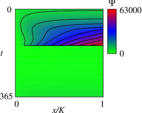
Figure 3. Computed reduced value function ${\mathrm{\Psi }}_1$. The contour lines represent 0.1, 0.2, 0.3, … 0.9 times of the maximum value of ${\mathrm{\Psi }}_1$ in the plotted area.

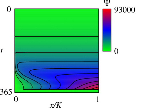
Figure 4. Computed sub-domains $D_{01}$ (Red) and $D_{10}$ (Blue).

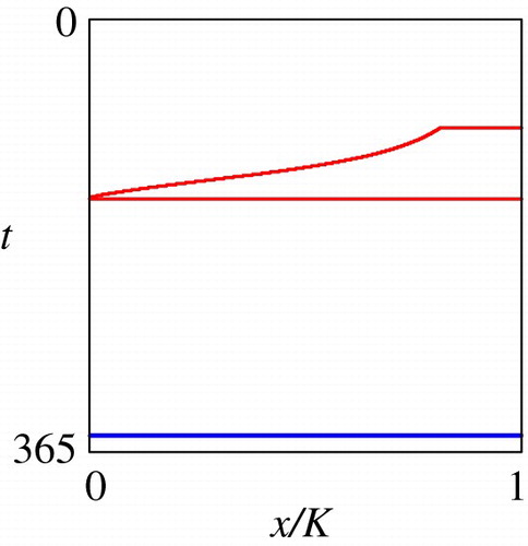
Figure 5. Dependence of the sub-domain $D_{01}$ on $R_0$.

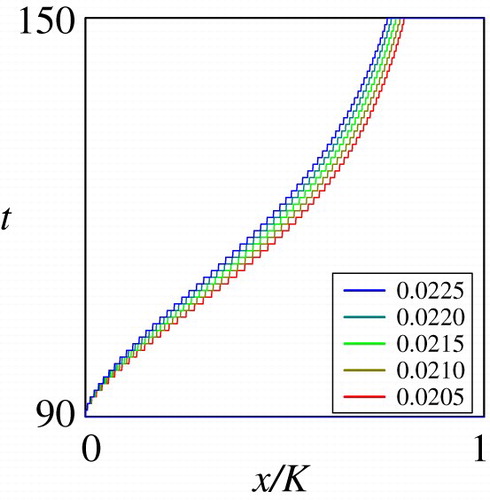
Figure 6. Dependence of the sub-domain $D_{01}$ on $r_0$.

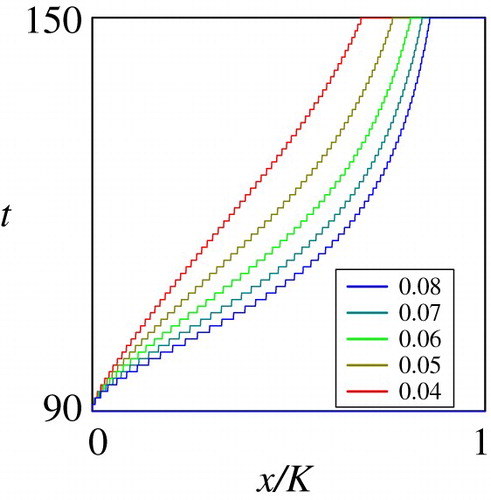
Figure 7. Dependence of the sub-domain $D_{01}$ on ${\sigma }_0$.

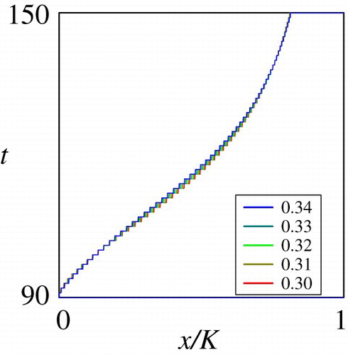
Figure 5 through Figure 7 show the dependence of the sub-domain $D_{01}$ on the mortality rate $R_0$, deterministic growth rate $r_0$, and the stochastic growth rate ${\sigma }_0$. These are key parameters shaping the juvenile life history of the fish in the habitat $H_0$. Figure 5 and Figure 6 show that the dependence of the optimal migration strategy from $H_0$ to $H_1$ is monotone on the parameters $R_0$ and $r_0$. The computational results on $R_0$ show that the migration occurs at an earlier growth stage if the mortality rate is higher in the habitat $H_0$, implying that a higher predation pressure may trigger an earlier migration. On the other hand, the computational results on $r_0$ indicate that a higher deterministic growth rate implies the migration at a later growth stage. Figure 7 shows that the dependence of the optimal migration strategy from $H_0$ to $H_1$would not be critically affected by the stochastic growth rate ${\sigma }_0$. However, the computational results on the basic reproduction number carried out in the next sub-section demonstrate that this parameter critically affects the reproduction success of the population eventually.

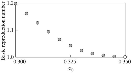
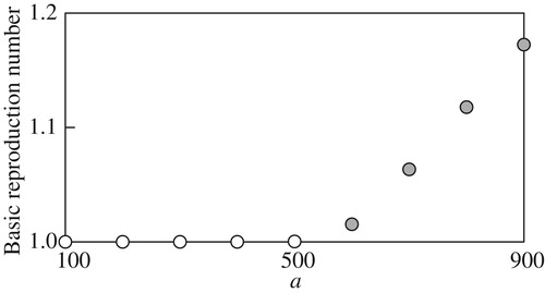
3.3.2 Basic reproduction number

The basic reproduction number $\mathcal{R}$ emerges when computing the value function and optimal migration strategy is computed for different parameter values. The computation here focus on the dependence of $\mathcal{R}$ on the life history during the juvenile period of the fish, which can be identified as the period that the population is living in the habitat $H_0$. Figure 8 through Figure 11 plot the basic reproduction number $\mathcal{R}$ against different values of the model parameters: the deterministic growth rate $r_0$ (1/day), the stochastic growth rate${\sigma }_0$ (1/day^1/2), the mortality rate $R_0$ (1/day), and the coefficient $a$ of fecundity, respectively. In these figures, the grey circles represent $\mathcal{R}>1$, while white circles represent $R=1$. Numerically, we found that $\mathcal{R}\ge 1$, suggesting that the case $0<\mathcal{R}<1$ can be excluded in practice, as implied in Remark 2.4.

Figure 8. The basic reproduction number $\mathcal{R}$ against different values of $r_0$ (1/day). The grey circles represent $\mathcal{R}>1$, while white circles represent $\mathcal{R}=1$.

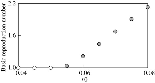
The computational results in Figure 8 through Figure 11 imply continuous and monotone dependence of $\mathcal{R}$ on the examined model parameters, and suggest that more reproduction success can be with higher deterministic growth, smaller growth fluctuations, smaller mortality, or higher fecundity. In addition, for each parameter, there seems to exist a threshold value above or below which the basic reproduction number $\mathcal{R}$ numerically equals 1. Therefore, from the standpoint of the present mathematical model, sustainability of the population dynamics would be suddenly abandoned if some parameter value crosses the threshold from the $\mathcal{R}>1$ side to the other side where $\mathcal{R}=1$. The computational result in Figure 9 is informative because it suggests $\mathcal{R}=1$ if $2{\mu }_0\le {\sigma }_0^2$ namely if ${\sigma }_0\ge 0.346$. Since $2{\mu }_0>{\sigma }_0^2$ is the condition that the body weight of the individuals increases as the time elapses (Theorem 2.2 of Lungu and Øksendal [80]), Figure 9 implies that the condition $2{\mu }_0>{\sigma }_0^2$ is required for sustainable population growth where $\mathcal{R}>1$. At the same time, the figure also implies that the sustainable population growth can be possibly achieved when under the stochastic environment if $2{\mu }_0>{\sigma }_0^2$.

Figure 9. The basic reproduction number $\mathcal{R}$ against different values of ${\sigma }_0$ (1/day^1/2). The grey circles represent $\mathcal{R}>1$, while white circles represent $\mathcal{R}=1$.

Overall, the computational results indicate critical importance of the environmental conditions during the juvenile period in the life history of the fish P. altivelis from the viewpoint of an SDP model: a new theoretical viewpoint. As demonstrated in this section, the present model can simulate the value function, the associated optimal migration strategy, and further sustainability of the population dynamics through the basic reproduction number $\mathcal{R}$ in a consistent way (Figure 10).

Figure 10. The basic reproduction number $\mathcal{R}$ against different values of ${\mathcal{R}}_0$ (1/day). The grey circles represent $\mathcal{R}>1$, while white circles represent $\mathcal{R}=1$.

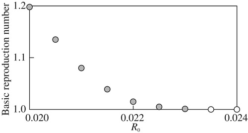
Figure 11. The basic reproduction number $\mathcal{R}$ against different values of $a$. The grey circles represent $\mathcal{R}>1$, while white circles represent $\mathcal{R}=1$.

4. Conclusions

An SDP formulation of migrating population dynamics between two habitats was proposed and was numerically computed based on the concept of stochastic optimal switching. The impulsive migration assumption combined with the population dynamics model effectively reduced finding the optimal migration strategy to solving the (reduced) optimality equation as a system of quasi-variational inequalities. The model is theoretically advantageous because solving the optimality equation directly gives the optimized objective function, the associated optimal migration strategy, and the basic reproduction number at once. A finite difference scheme was implemented in numerical computation of the model focusing on an application to P. altivelis. The computational results implied dependence of the reproduction success on the model parameters. We demonstrated that the optimal switching formalism serves as a new mathematical tool that enables us to describe the state-dependent, and thus adaptive migration dynamics of population based on biological and environmental conditions. We used a logistic model for describing the biological growth, but the other models like the classical von Bertalanffy model [99] can be used alternatively within our mathematical framework. The resulting optimality equation will be different from ours in such a case, but the numerical technique will be applicable because the equation will still be a system of degenerate parabolic variational inequalities.

There are diverse extensions of the current mathematical model. The density-dependence ignored in this paper can be considered at the cost of increase of the complexity. Approaching the optimization part from a fitness viewpoint may open the door toward a new mathematical modelling to consider evolutionary stable migration strategies. The current model can be extended so that population dynamics having an age structure [100,101] is handled if the variables depending on the age-class are specified. Problems where the population migrates among more than two habitats [62] can also be handled through an increase of the total number of states using a Markov chain technique [61]. Considering the other biological scaling relationships for reproduction and mortality would enable the current model to handle migrating population dynamics of different species. Application of the current the model to predator-prey population dynamics will be feasible through considering a seasonal prey availability [77]. The current model can also be applied to population dynamics facing with environmental uncertainty [57], which can be theoretically achieved through considering the zero-sum differential game formulation [102] between the population and nature. Another advanced problem will be how to formulate migrating population dynamics where qualitatively different (for example, impulsive or gradual) migration strategies may arise depending on the environmental conditions [90]. Mathematical analysis of the model from the viewpoint of viscosity solutions to degenerate parabolic equations having a discontinuous Hamiltonian [103] is an important research topic from a mathematical viewpoint. Resolving this issue will deepen understanding of the model. From a management side, it is important to establish a harvesting policy and a habitat management policy considering sustainability of the fish population, so that the basic reproduction number is always greater than one. Currently, we are considering an application of the present model to modelling a life cycle of land-locked P. altivelis in Japan migrating between a reservoir and its upstream river.

Acknowledgement

The authors thank Dr. Marc Mangel for his valuable comments and suggestions based on evolutionary biology and fish migration, which significantly improved our research.

Disclosure statement

No potential conflict of interest was reported by the authors.

ORCID

Hidekazu Yoshioka http://orcid.org/0000-0002-5293-3246

Additional information

Funding

JSPS Research Grant 19H03073 and a grant for ecological survey of a life history of the landlocked Ayu Plecoglossus altivelis altivelis from MLIT of Japan support this research.

Appendix A

Proofs of Propositions 2.1 and 2.2 are presented in this appendix.

Proof

Proof of Proposition 2.1

The non-negativity of $\mathrm{\Phi }$ is trivial by the definition. On the other hand, we have (37) $\begin{array}{rl}\mathrm{\Phi }\left(t,n,x,l\right)& =\underset{\tau \in \mathcal{T}}{sup}{\mathbb{E}}_{n,x,l}\left[w\sum _{k=k_{min}}^{k_{max}}a{S}_{10}{X}_{{\tau }_{10}^{\left(k\right)}}^b{N}_{{\tau }_{10}^{\left(k\right)}}\right]\\ & \le wa{S}_{10}{K}^b\underset{\tau \in \mathcal{T}}{sup}{\mathbb{E}}_{n,x,l}\left[\sum _{k=k_{min}}^{k_{max}}{N}_{{\tau }_{10}^{\left(k\right)}}\right]\\ & \le wa{S}_{10}{K}^b\underset{\tau \in \mathcal{T}}{sup}{\mathbb{E}}_{n,x,l}\left[\sum _{k=k_{min}}^{k_{max}}n{\left(S_{10}a{K}^b\right)}^{k-1}\right]\\ & =Cn\end{array}$(37) with $0<C=w\sum _{k=k_{min}}^{k_{max}}n{\left(S_{10}a{K}^b\right)}^{k-1}<+\mathrm{\infty }$.

Proof

Proof of Proposition 2.2

Firstly, the Lipschitz continuity with respect to $n\ge 0$ is trivial because of the relationship $\mathrm{\Phi }\left(t,n,x,l\right)=n\mathrm{\Psi }\left(t,x,l\right)$ and $\mathrm{\Psi }\left(t,x,l\right)$ is bounded by Proposition 2.1.

Secondly, the Lipschitz continuity with respect to $0\le x\le K$ is proven as follows. The process $X_s$ ($s\ge t$) subject to $X_{t-0}=x\in \left[0,K\right]$ is denoted as $X_s^{\left(t,x\right)}$. Then, for $0\le x,y\le K$ and $\tau \in \mathcal{T}$, there exists a constant $C>0$ such that (38) $\begin{array}{rl}|\phi \left(t,n,x,l;\tau \right)-\phi \left(t,n,y,l;\tau \right)|& \le C\mathbb{E}\left[\sum _{k=k_{min}}^{k_{max}}|{\left(X_{{\tau }_{10}^{\left(k\right)}}^{\left(t,x\right)}\right)}^b-{\left(X_{{\tau }_{10}^{\left(k\right)}}^{\left(t,y\right)}\right)}^b|\right]\\ & \le bC{K}^{b-1}\sum _{k=k_{min}}^{k_{max}}\mathbb{E}\left[|X_{{\tau }_{10}^{\left(k\right)}}^{\left(t,x\right)}-X_{{\tau }_{10}^{\left(k\right)}}^{\left(t,y\right)}|\right]\end{array}$(38) by $b\ge 1$. Then, by the strong solution property of $X_s^{\left(t,x\right)}$, following, for some constant $C^{\mathrm{\prime }}>0$, we have (39) $|\phi \left(t,n,x,l;\tau \right)-\phi \left(t,n,y,l;\tau \right)|\le bC{K}^{b-1}\exp \left(C^{\mathrm{\prime }}T\right)|x-y|$(39) The Lipschitz continuity of $\mathrm{\Phi }$ immediately follows from (39) because $0\le x,y\le K$ and $\tau \in \mathcal{T}$ are chosen arbitrary.

Finally, the continuity with respect to $t$ is proven as follows. Set $l=1$. The proof for $l=0$ is proven in a similar way. Firstly, assume that $t$ is inside of $M_{10}^{\left(k\right)}$. Then, the continuity of $\mathrm{\Phi }\left(t,n,x,1\right)$ is proven following Theorem 3.1 of Tang and Yong [104]. The proof for $\mathrm{\Phi }\left(t,n,x,0\right)$ is a straightforward consequence of the fact that the state switching from $I_t=0$ to $I_t=1$ not allowed if $t$ is inside of $M_{10}^{\left(k\right)}$. Essentially the same argument applies to $t$is inside of $M_{01}^{\left(k\right)}$. The proof for $t$ outside of both $M_{01}^{\left(k\right)}$ and $M_{10}^{\left(k\right)}$ is straightforward as well since no state switching is allowed in such a case.

References

- J.J. Horns, and ÇH Şekercioğlu, Conservation of migratory species. Current Biol. 28 (2018), pp. R980–R983. doi:10.1016/j.cub.2018.06.032.
- C. S. Teitelbaum, and T. Mueller, Beyond migration: causes and consequences of nomadic animal movements. Trends Ecol. Evol. (2019).
- M. Goulding, Venticinque Eduardo, Ribeiro Mauro L. de B., Barthem Ronaldo B., Leite Rosseval G., Forsberg Bruce, Petry Paulo, Lopes da Silva-Júnior Urbano, Ferraz Polliana Santos, Cañas Carlos Ecosystem-based management of Amazon fisheries and wetlands. Fish Fisher. 20 (2019), pp. 138–158. doi:10.1111/faf.12328.
- Z. Tonkin, Lyon Jarod P., Moloney Paul, Balcombe Stephen R., Hackett Graeme, Spawning-stock characteristics and migration of a lake-bound population of the endangered Macquarie perch Macquaria australasica. J. Fish Biol. 93 (2018), pp. 630–640. doi:10.1111/jfb.13731.
- S. Bauer, Shamoun-Baranes Judy, Nilsson Cecilia, Farnsworth Andrew, Kelly Jeffrey F., Reynolds Don R., Dokter Adriaan M., Krauel Jennifer F., Petterson Lars B., Horton Kyle G., Chapman Jason W, The grand challenges of migration ecology that radar aeroecology can help answer. Ecography 42 (2019), pp. 861–875. doi:10.1111/ecog.04083.
- M. Minter, Pearson Aislinn, Lim Ka S., Wilson Kenneth, Chapman Jason W., Jones Christopher M., The tethered flight technique as a tool for studying life-history strategies associated with migration in insects. Ecol. Entomol. 43 (2018), pp. 397–411. doi:10.1111/een.12521.
- C. Ioannidou, and J.R. O’Hanley, The importance of spatiotemporal fish population dynamics in barrier mitigation planning. Biol. Conserv. 231 (2019), pp. 67–76. doi:10.1016/j.biocon.2019.01.001.
- R.A. McManamay, J.S. Perkin, and H.I. Jager, Commonalities in stream connectivity restoration alternatives: an attempt to simplify barrier removal optimization. Ecosp here. 10 (2019), pp. e02596. doi:10.1002/ecs2.2596.
- S. Bernardi, A. Colombi, and M. Scianna, A particle model analysing the behavioural rules underlying the collective flight of a bee swarm towards the new nest. J. Biol. Dynam. 12 (2018), pp. 632–662. doi:10.1080/17513758.2018.1501105.
- S. Steingass, and M. Horning, Individual-based energetic model suggests bottom up mechanisms for the impact of coastal hypoxia on Pacific harbor seal (Phoca vitulina richardii) foraging behavior. J. Theor. Biol. 416 (2017), pp. 190–198. doi:10.1016/j.jtbi.2017.01.006.
- I.T. Heilmann, U.H. Thygesen, and M.P. Sørensen, Spatio-temporal pattern formation in predator-prey systems with fitness taxis. Ecol. Complex 34 (2018), pp. 44–57. doi:10.1016/j.ecocom.2018.04.003.
- N.G. Marculis, and R. Lui, Modelling the biological invasion of Carcinus maenas (the European green crab). J. Biol. Dynam. 10 (2016), pp. 140–163. doi:10.1080/17513758.2015.1115563.
- R. Lande, S. Engen, and B.E. Saether, Stochastic Population Dynamics in Ecology and Conservation, Oxford University Press on Demand, Oxford, 2003.
- H.R. Thieme, Mathematics in Population Biology, Princeton University Press, Princeton, 2018.
- H. Yoshioka, Mathematical analysis and validation of an exactly solvable model for upstream migration of fish schools in one-dimensional rivers. Math. Biosci. 281 (2016), pp. 139–148. doi:10.1016/j.mbs.2016.09.014.
- H. Yoshioka, A simple game-theoretic model for upstream fish migration. Theor. Biosci. 136 (2017), pp. 99–111. doi:10.1007/s12064-017-0244-3.
- H. Ito, Risk sensitivity of a forager with limited energy reserves in stochastic environments. Ecol. Res. 34 (2019), pp. 9–17. doi:10.1111/1440-1703.1058.
- Y. Sato, K. Ito, and H. Kudoh, Optimal foraging by herbivores maintains polymorphism in defence in a natural plant population. Funct. Ecol. 31 (2017), pp. 2233–2243. doi:10.1111/1365-2435.12937.
- E.Y. Frisman, G.P. Neverova, and M.P. Kulakov, Change of dynamic regimes in the population of species with short life cycles: results of an analytical and numerical study. Ecol. Complex 27 (2016), pp. 2–11. doi:10.1016/j.ecocom.2016.02.001.
- A.M. Yousef, Stability and further analytical bifurcation behaviors of Moran-Ricker model with delayed density dependent birth rate regulation. J. Comput. Appl. Math. 355 (2019), pp. 143–161. doi:10.1016/j.cam.2019.01.012.
- A.I. Houston, and J.M. McNamara, Models of Adaptive Behaviour: An Approach Based on State, Cambridge Univ. Press, Cambridge.
- M. Mangel, Stochastic dynamic programming illuminates the link between environment, physiology, and evolution. Bull. Math. Biol. 77 (2015), pp. 857–877. doi:10.1007/s11538-014-9973-3.
- M. Assid, A. Gharbi, and A. Hajji, Production and setup control policy for unreliable hybrid manufacturing-remanufacturing systems. J. Manufactur. Syst. 50 (2019), pp. 103–118. doi:10.1016/j.jmsy.2018.12.004.
- H. Rivera-Gómez, Gharbi Ali, Kenné Jean-Pierre, Montaño-Arango Oscar, Hernández-Gress Eva Selene, Subcontracting strategies with production and maintenance policies for a manufacturing system subject to progressive deterioration. Int. J. Prod. Econ. 200 (2018), pp. 103–118. doi:10.1016/j.ijpe.2018.03.004.
- L. Bo, A. Capponi, and P.C. Chen, Credit portfolio selection with decaying contagion intensities. Math. Financ. 29 (2019), pp. 137–173. doi:10.1111/mafi.12177.
- J. Wang, P. Zhao, and Q. Gao, Portfolio selection problem with nonlinear wealth equations under non-extensive statistical mechanics for time-varying SDE. Comput. Math. Appl. 77 (2019), pp. 555–564. doi:10.1016/j.camwa.2018.09.057.
- Y. Dong, and H. Zheng, Optimal investment of DC pension plan under short-selling constraints and portfolio insurance. Insur. Math. Econ. 85 (2019), pp. 47–59. doi:10.1016/j.insmatheco.2018.12.005.
- X. Xue, P. Wei, and C. Weng, Derivatives trading for insurers. Insur. Math. Econ. 84 (2019), pp. 40–53. doi:10.1016/j.insmatheco.2018.11.001.
- M.C. Insley, Resource extraction with a carbon tax and regime switching prices. Ener. Econ. 67 (2017), pp. 1–16. doi:10.1016/j.eneco.2017.07.013.
- F. van der Ploeg, and A. de Zeeuw, Pricing carbon and adjusting capital to fend off climate catastrophes. Environ. Resour. Econ. 72 (2019), pp. 29–50. doi:10.1007/s10640-018-0231-2.
- Y. Yaegashi, H. Yoshioka, K. Unami, and M. Fujihara, A singular stochastic control model for sustainable population management of the fish-eating waterfowl Phalacrocorax carbo. J. Environ. Manage. 219 (2018), pp. 18–27. doi:10.1016/j.jenvman.2018.04.099.
- H. Yoshioka, A simplified stochastic optimization model for logistic dynamics with control-dependent carrying capacity. J. Biol. Dynam. 13 (2019a), pp. 148–176. doi:10.1080/17513758.2019.1576927.
- B. Vardar, and G. Zaccour, The strategic impact of adaptation in a transboundary pollution dynamic game. Environ. Model. Assess. 23 (2018), pp. 653–669. doi:10.1007/s10666-018-9616-4.
- H. Yoshioka, Y. Yaegashi, Y. Yoshioka, and K. Hamagami, Hamilton–jacobi–bellman quasi-variational inequality arising in an environmental problem and its numerical discretization. Comput. Math. Appl. 77 (2019a), pp. 2182–2206. doi:10.1016/j.camwa.2018.12.004.
- M. Mangel, and C.W. Clark, Dynamic Modeling in Behavioral Ecology, Princeton University Press, Princeton.
- E.A. McHuron, L.K. Schwarz, D.P. Costa, and M. Mangel, A state-dependent model for assessing the population consequences of disturbance on income-breeding mammals. Ecol. Model. 385 (2018), pp. 133–144. doi:10.1016/j.ecolmodel.2018.07.016.
- A. Brodin, JÅ Nilsson, and A. Nord, Adaptive temperature regulation in the little bird in winter: predictions from a stochastic dynamic programming model. Oecologia 185 (2017), pp. 43–54. doi:10.1007/s00442-017-3923-3.
- J. van den Heuvel, Saastamoinen Marjo, Brakefield Paul M., Kirkwood Thomas B. L., Zwaan Bas J., Shanley Daryl P., The predictive adaptive response: modeling the life-history evolution of the butterfly Bicyclus anynana in seasonal environments. Am. Nat. 181 (2013), pp. E28–E42. doi:10.1086/668818.
- A.M. Frame, and A.F. Mills, Condition-dependent mate choice: a stochastic dynamic programming approach. Theor. Popul. Biol. 96 (2014), pp. 1–7. doi:10.1016/j.tpb.2014.06.001.
- B.D. Griffen, Reproductive skipping as an optimal life history strategy in the southern elephant seal, Mirounga leonina. Ecol. Evol. 8 (2018), pp. 9158–9170. doi:10.1002/ece3.4408.
- J. Purcell, and A. Brodin, Factors influencing route choice by avian migrants: a dynamic programming model of Pacific brant migration. J. Theor. Biol. 249 (2007), pp. 804–816. doi:10.1016/j.jtbi.2007.08.028.
- A. Ez-zizi, J.M. McNamara, G. Malhotra, and A.I. Houston, Optimal gut size of small birds and its dependence on environmental and physiological parameters. J. Theor. Biol. 454 (2018), pp. 357–366. doi:10.1016/j.jtbi.2018.05.010.
- M. Schaefer, S. Menz, F. Jeltsch, and D. Zurell, sOAR: a tool for modelling optimal animal life-history strategies in cyclic environments. Ecography 41 (2018), pp. 551–557. doi:10.1111/ecog.03328.
- W.H. Satterthwaite, Hayes Sean A., Merz Joseph E., Sogard Susan M., Frechette Danielle M., Mangel Marc, State-dependent migration timing and use of multiple habitat types in anadromous salmonids. Trans. Am. Fisher. Soc. 141 (2012), pp. 781–794. doi:10.1080/00028487.2012.675912.
- B.K. Øksendal, and A. Sulem, Applied Stochastic Control of Jump Diffusions, Springer, Berlin, 2007.
- H. Pham, Continuous-Time Stochastic Control and Optimization with Financial Applications, Springer Science & Business Media, Dordrecht, 2009.
- H. Yoshioka, and Y. Yaegashi, Singular stochastic control model for algae growth management in dam downstream. J. Biol. Dynam. 12 (2018a), pp. 242–270. doi:10.1080/17513758.2018.1436197.
- S.P. Zhu, and G. Ma, An analytical solution for the HJB equation arising from the Merton problem. Int. J. Financ. Eng. 5 (2018), pp. 1850008. doi:10.1142/S2424786318500081.
- J. Lai, J.W. Wan, and S. Zhang, Numerical methods for two person games arising from transboundary pollution with emission permit trading. Appl. Math. Comput. 350 (2019), pp. 11–31.
- C. Parzani, and S. Puechmorel, On a Hamilton-jacobi-bellman approach for coordinated optimal aircraft trajectories planning. Optim. Contr. Appl. Method 39 (2018), pp. 933–948. doi:10.1002/oca.2389.
- A. Barth, S. Moreno–Bromberg, and O. Reichmann, A non-stationary model of dividend distribution in a stochastic interest-rate setting. Comput. Econ. 47 (2016), pp. 447–472. doi:10.1007/s10614-015-9502-y.
- C. Wang, and J. Wang, A primal-dual weak Galerkin finite element method for second order elliptic equations in non-divergence form. Math. Comput. 87 (2018), pp. 515–545. doi:10.1090/mcom/3220.
- J. Alonso-García, O. Wood, and J. Ziveyi, Pricing and hedging guaranteed minimum withdrawal benefits under a general Lévy framework using the COS method. Quant. Financ. 18 (2018), pp. 1049–1075. doi:10.1080/14697688.2017.1357832.
- P. Forsyth, and G. Labahn, ε-monotone Fourier methods for optimal stochastic control in finance. J. Comput. Financ. 22:4. https://ssrn.com/abstract=3341491. doi: 10.21314/JCF.2018.361
- U.H. Thygesen, L. Sommer, K. Evans, and T.A. Patterson, Dynamic optimal foraging theory explains vertical migrations of bigeye tuna. Ecology 97 (2016), pp. 1852–1861. doi:10.1890/15-1130.1.
- U.H. Thygesen, and T.A. Patterson, Oceanic diel vertical migrations arising from a predator-prey game. Theor. Ecol. 12 (2019), pp. 17–29. doi:10.1007/s12080-018-0385-0.
- H. Yoshioka, A stochastic differential game approach toward animal migration. Theor. Biosci. 2019b.
- H. Yoshioka, and Y. Yaegashi, An optimal stopping approach for onset of fish migration. Theor. Biosci 137 (2018b), pp. 99–116. doi:10.1007/s12064-018-0263-8.
- M.J. Ejsmond, J.M. McNamara, J. Søreide, and Ø Varpe, Gradients of season length and mortality risk cause shifts in body size, reserves and reproductive strategies of determinate growers. Funct. Ecol. 32 (2018), pp. 2395–2406. doi:10.1111/1365-2435.13191.
- J. Johansson, Å Brännström, J.A. Metz, and U. Dieckmann, Twelve fundamental life histories evolving through allocation-dependent fecundity and survival. Ecol. Evol. 8 (2018), pp. 3172–3186. doi:10.1002/ece3.3730.
- A. Kölzsch, E. Kleyheeg, H. Kruckenberg, M. Kaatz, and B. Blasius, A periodic Markov model to formalize animal migration on a network. Royal Soc. Open Sci. 5 (2018), pp. 180438. doi:10.1098/rsos.180438.
- P. Mariani, V. Křivan, B.R. MacKenzie, and C. Mullon, The migration game in habitat network: the case of tuna. Theor. Ecol. 9 (2016), pp. 219–232. doi:10.1007/s12080-015-0290-8.
- C.M. Taylor, A.J. Laughlin, and R.J. Hall, The response of migratory populations to phenological change: a migratory flow network modelling approach. J. Animal Ecol 85 (2016), pp. 648–659. doi:10.1111/1365-2656.12494.
- D. Z. Szabó, P. Duck, P. Johnson, Optimal trading of imbalance options for power systems using an energy storage device, in press. Euro. J. Oper. Res.
- G. Shim, J.L. Koo, and Y.H. Shin, Reversible job-switching opportunities and portfolio selection. Appl. Math. Optim. 77 (2018), pp. 197–228. doi:10.1007/s00245-016-9371-3.
- K. Suzuki, Optimal switching strategy of a mean-reverting asset over multiple regimes. Automatica. (Oxf) 67 (2016), pp. 33–45. doi:10.1016/j.automatica.2015.12.023.
- B. El Asri, and S. Mazid, Stochastic differential switching game in infinite horizon. J. Math. Anal. Appl 474 (2019), pp. 793–813. doi:10.1016/j.jmaa.2019.01.040.
- J.M. Cushing, and O. Diekmann, The many guises of R0 (a didactic note). J Theor. Biol. 404 (2016), pp. 295–302. doi:10.1016/j.jtbi.2016.06.017.
- D. Miyadi, The Ayu, Iwanami Shoten, Tokyo, 1960. (in Japanese).
- H. Yoshioka, and Y. Yaegashi, Stochastic differential game for management of non-renewable fishery resource under model ambiguity. J. Biol. Dynam. 12 (2018c), pp. 817–845. doi:10.1080/17513758.2018.1528394.
- K.I. Iguchi, Egg size plasticity corresponding to maternal food conditions in an annual fish, Ayu Plecoglossus altivelis. Ichthyol. Res. 59 (2012), pp. 14–19. doi:10.1007/s10228-011-0246-y.
- Japan Fisheries Resource Conservation Association (1998) Plecoglossus altivelis altivelis (Ayu), published by Japan Fisheries Resource Conservation Association, Tokyo. (in Japanese).
- H. Yoshioka, Y. Yaegashi, Y. Yoshioka, and K. Tsugihashi, Optimal harvesting policy of an inland fishery resource under incomplete information. Appl. Stoch. Model. Bus 35 (2019), pp. 939–962. 10.1002/asmb.2428. doi: 10.1002/asmb.2428
- B.M. Gillanders, C. Izzo, Z.A. Doubleday, and Q. Ye, Partial migration: growth varies between resident and migratory fish. Biol. Lett. 11 (2015), pp. 20140850. doi:10.1098/rsbl.2014.0850.
- T. Arai, H. Hayano, H. Asami, and N. Miyazaki, Coexistence of anadromous and lacustrine life histories of the shirauo. Fisher. Oceanogra. 12 (2003), pp. 134–139. doi:10.1046/j.1365-2419.2003.00226.x.
- T. Arai, J. Yang, and N. Miyazaki, Migration flexibility between freshwater and marine habitats of the pond smelt Hypomesus nipponensis. J. Fish Biol 68 (2006), pp. 1388–1398. doi:10.1111/j.0022-1112.2006.01002.x.
- J.G. Donohue, and P.T. Piiroinen, Mathematical modelling of seasonal migration with applications to climate change. Ecol. Model 299 (2015), pp. 79–94. doi:10.1016/j.ecolmodel.2014.12.003.
- J.G. Donohue, and P.T. Piiroinen, The effects of predation on seasonally migrating populations. Theor. Ecol. 9 (2016), pp. 487–499. doi:10.1007/s12080-016-0304-1.
- M.A. Gil, Hein Andrew M., Spiegel Orr, Baskett Marissa L., Sih Andrew, Social information links individual behavior to population and community dynamics. Trends Ecol. Evol. 33 (2018), pp. 535–548. doi:10.1016/j.tree.2018.04.010.
- E.M. Lungu, and B. Øksendal, Optimal harvesting from a population in a stochastic crowded environment. Math. Biosci. 145 (1997), pp. 47–75. doi:10.1016/S0025-5564(97)00029-1.
- T. Azuma, Noda Shuhei, Yada Takashi, Ototake Mitsuru, Nagoya Hiroiyuki, Moriyama Shunsuke, Yamada Hideaki, Nakanishi Teruyuki, Iwata Munehico, Profiles in growth, smoltification, immune function and swimming performance of 1-year-old masu salmon Oncorhynchus masou masou reared in water flow. Fisher. Sci. 68 (2012), pp. 1282–1294. doi:10.1046/j.1444-2906.2002.00566.x.
- K.L. Bellinger, G.H. Thorgaard, and P.A. Carter, Complex relationships among rearing temperature, growth, and sprint speed in clonal lines of rainbow trout. Can. J. Fisher. Aquat. Sci. 75 (2018), pp. 1868–1877. doi:10.1139/cjfas-2017-0218.
- P.E. Hirsch, M. Thorlacius, T. Brodin, and P. Burkhardt-Holm, An approach to incorporate individual personality in modeling fish dispersal across in-stream barriers. Ecol. Evol. 7 (2017), pp. 720–732. doi:10.1002/ece3.2629.
- C.M. Alexandre, and A.P. Palstra, Effect of short-term regulated temperature variations on the swimming economy of Atlantic salmon smolts. Conserv. Physiol. 5 (2017), pp. cox025. doi:10.1093/conphys/cox025.
- S. Nakamura, Gyodou no Hanashi (Story of Fishway), Sankai-do, Tokyo, 1995. (in Japanese).
- D.R. Barneche, D.R. Robertson, C.R. White, and D.J. Marshall, Fish reproductive-energy output increases disproportionately with body size. Science 360 (2018), pp. 642–645. https://10.1126/science.aao6868.
- A.J. Hendriks, and C. Mulder, Scaling of offspring number and mass to plant and animal size: model and meta-analysis. Oecologia 155 (2008), pp. 705–716. doi:10.1007/s00442-007-0952-3.
- D.J. Marshall, and C.R. White, Have we outgrown the existing models of growth? Trends Ecol. Evol. 34 (2018), pp. 102–111. doi:10.1016/j.tree.2018.10.005.
- K. Omori, Ohnishi Hidejiro, Hamaoka Hideki, Kunihiro Tadao, Ito Sayaka, Kuwae Michinobu, Hata Hiroki, Miller Todd W., Iguchi Keiichiro, Speciation of fluvial forms from amphidromous forms of migratory populations. Ecol. Model 243 (2012), pp. 89–94. doi:10.1016/j.ecolmodel.2012.06.006.
- J. Horita, Y. Iwasa, and Y. Tachiki, Evolutionary bistability of life history decision in male masu salmon. J. Theor. Biol. 448 (2018), pp. 104–111. doi:10.1016/j.jtbi.2018.04.008.
- B. Jonsson, M. Jonsson, and N. Jonsson, Optimal size at seaward migration in an anadromous salmonid. Mar. Ecol. Prog. Ser. 559 (2016), pp. 193–200. doi:10.3354/meps11891.
- B. Jonsson, M. Jonsson, and N. Jonsson, Influences of migration phenology on survival are size-dependent in juvenile Atlantic salmon (Salmo salar). Can. J. Zool. 95 (2017), pp. 581–587. doi:10.1139/cjz-2016-0136.
- M.G. Crandall, H. Ishii, and P.L. Lions, User’s guide to viscosity solutions of second order partial differential equations. Bull. Am. Math. Soc. 27 (1992), pp. 1–67. doi:10.1090/S0273-0979-1992-00266-5.
- S. Lv, Z. Wu, and Q. Zhang, Optimal switching under a hybrid diffusion model and applications to stock trading. Automatica. (Oxf) 94 (2018), pp. 361–372. doi:10.1016/j.automatica.2018.04.048.
- G. Barles, and E. Chasseigne, An illustrated guide of the modern approches of Hamilton-Jacobi equations and control problems with discontinuities. arXiv Preprint arXiv (2018), pp. 1812.09197.
- P. Azimzadeh, E. Bayraktar, and G. Labahn, Convergence of implicit schemes for Hamilton-Jacobi-Bellman quasi-variational inequalities. SIAM J. Control. Optim. 56 (2018), pp. 3994–4016. doi:10.1137/18M1171965.
- P.A. Forsyth, K.R. Vetzal, Numerical methods for nonlinear PDEs in finance, in Handbook of Computational Finance, Duan J. C., Hardle W., Gentle J., eds., Springer, Berlin, 2012. pp. 503–528.
- G. Barles P, and E. Souganidis, Convergence of approximation schemes for fully nonlinear second order equations. Asympt. Anal 4 (1991), pp. 271–283.
- C. Vincenzi, A.J. Crivelli, S. Munch, H.J. Skaug, and M. Mangel, Trade-offs between accuracy and interpretability in von Bertalanffy random-effects models of growth. Ecol. Appl. 26 (2016), pp. 1535–1552. doi:10.1890/15-1177.
- L.G. Crozier, R.W. Zabel, and A.F. Hamlet, Predicting differential effects of climate change at the population level with life-cycle models of spring Chinook salmon. Global Change Biol. 14 (2008), pp. 236–249. doi:10.1111/j.1365-2486.2007.01497.x.
- R. Kentie, Coulson Tim, Hooijmeijer Jos C. E. W., Howison Ruth A., Loonstra A. H. Jelle, Verhoeven Mo A., Both Christiaan, Piersma Theunis, Warming springs and habitat alteration interact to impact timing of breeding and population dynamics in a migratory bird. Global Change Biol. 24 (2017), pp. 5292–5303. doi:10.1111/gcb.14406.
- L. Hansen, and T.J. Sargent, Robust control and model uncertainty. Am. Econ. Rev 91 (2001), pp. 60–66. doi:10.1257/aer.91.2.60.
- G.M. Coclite, and N.H. Risebro, Viscosity solutions of Hamilton–jacobi equations with discontinuous coefficients. Jo Hyperbolic Differ. Equat 4 (2017), pp. 771–795. doi:10.1142/S0219891607001355.
- S. Tang, and J. Yong, Finite horizon stochastic optimal switching and impulse controls with a viscosity solution approach. Stochastics 45 (1993), pp. 145–176.