Stability of a certain class of a host–parasitoid models with a spatial refuge effect

Abstract

A certain class of a host–parasitoid models, where some host are completely free from parasitism within a spatial refuge is studied. In this paper, we assume that a constant portion of host population may find a refuge and be safe from attack by parasitoids. We investigate the effect of the presence of refuge on the local stability and bifurcation of models. We give the reduction to the normal form and computation of the coefficients of the Neimark–Sacker bifurcation and the asymptotic approximation of the invariant curve. Then we apply theory to the three well-known host–parasitoid models, but now with refuge effect. In one of these models Chenciner bifurcation occurs. By using package Mathematica, we plot bifurcation diagrams, trajectories and the regions of stability and instability for each of these models.

Keywords:

• Chenciner bifurcation
• host–parasitoid
• invariant curve
• Neimark–Sacker bifurcation
• refuge effect

2010 Mathematics Subject Classifications:

• 39A10
• 39A30
• 39A28
• 92D25

1. Introduction

A model which has received considerable attention from experimental and theoretical biologists is the host–parasitoid system, see [3]. In mathematical biology, the host–parasitoid interactions are very popular subjects since they are important to address the natural enemy of an insect pest.

Parasitoids are insect species of which larvae develop as parasites on other insect species. Parasitoid larvae usually kill their host (sometimes the host is paralyzed by the ovipositing parasitoid female) whereas adult parasitoids are free-living insects. Parasitoids and their hosts often have synchronized life-cycles, e.g. both have one generation per year (monovoltinous). Thus, host–parasitoid model usually use discrete time steps that correspond generations. Most parasitoid species are either wasps or flies.

Many authors have investigated different types of discrete host–parasitoid models under different ecological factors and different assumptions, see for example [1,7,12–14,18–21,23,24,28].

For the host–parasitoid model of Nicholson–Bailey, the basic variables and parameters are defined as follows: $N_n$ is density of host species in generation n, $P_n$ is density of parasitoid species in generation n, $F(N_n,P_n)$ is fraction of hosts not parasitized, r is number of eggs laid by a host that survive through the larvae, pupae, and adult stages, e is number of eggs laid by a parasitoid on a single host that survive through larvae, pupae, and adult stages. See [14]. The parameter r and e are positive. Applying these definitions, the general host–parasitoid model has the following form: $\begin{array}{rl}{H}_{n+1}& =r{H}_{n}F(H_n,P_n)\\ P_{n+1}& =e{H}_n(1-F(H_n,P_n\left)\right).\end{array}$ The first host–parasitoid model was proposed by Thompson in 1924, see [29]. The model of Thompson assumes that female parasitoids lay their legs randomly on host individual and are unable to distinguish unparasitized individuals of the host species and individuals already parasitized. In the model of Thompson it is assumed that parasitoids always lay all their legs, that is realized fecundity equals potential fecundity. This implies that there are unlimited search abilities of parasitoids. However, in nature usually parasitoids do not realize their potential fecundity because they can not find enough hosts. Thus, the model of Thompson may overestimate parasitism rates especially if host density is low. The dynamics of the generalization of Thompson's model is investigated in [27]. This generalization includes host density dependence and aggregation of parasitoid attacks. This model assumes that parasitoids are egg-limited but not search limited.

In 1935, Nicholson and Bailey proposed more realistic model, in the sequel $\left(NB\right)$ model, than Thompson's model, see [2]: $\begin{array}{rl}{H}_{n+1}& =r{H}_n{\mathrm{e}}^{-d{P}_n}\\ P_{n+1}& =e{H}_n(1-{\mathrm{e}}^{-d{P}_n}),\end{array}$ where d representing the ‘area of discovery’ or the proportion of the host environment that can be covered by an individual parasitoid in its lifetime. This is a discrete time model of a biological system involved two insects, a parasitoid and its host. This model assumes that parasitoid female is able to examine area during its life time. When a host is found, parasitoid lays only one egg in it. However, the same host can be found again later and then the parasitoid will lay another egg in it because it is assumed that parasitoid does not distinguish unparasitized and parasitized individuals of the host species. In the Nicholson–Bailey model, the potential fecundity of parasitoids is not limited. Parasitoides lay an egg at every encounter with the host even if the number of encounters is very large, that is if host density is high. This model is one of the well-known models for many experimental and theoretical investigations in ecology.

In 1972, Rogers proposed the model which applies the model of Holling, that was originally developed for predator–pray systems, to host–parasitoid model, see [10,25]. This model assumes two kind of limitations in host–parasitoid interactions. These limitations are: limited parasitoid fecundity (as in Thompson's model [29]) and limited search rate (as in the model of Bailey and Nicholson [2]).

The following model was investigated by Lauwerier and Metz [17]: $\begin{array}{rl}{H}_{n+1}& =r{H}_{n}f\left(P_n\right)\\ P_{n+1}& =r{H}_n(1-f(P_n\left)\right),\end{array}$ where $f\left(y\right)$ is assumed to be differentiable with $f^{\prime }\left(y\right)<0$, $f\left(0\right)=r$, and $f\left(\mathrm{\infty }\right)<1$. Lauwerier and Metz applied the theory to the following four cases.

1. $\left(S\right)$-simple model: $f\left(y\right)=\frac{1}{1+y^m}$, m>0

2. $\left(HV\right)$ model: $f\left(y\right)={\mathrm{e}}^{-y^m}$, $0<m\le 1$ (Hassell and Varley, 1969 [9]),

3. $\left(PP\right)$ model: $f\left(y\right)={\mathrm{e}}^{-\frac{\sqrt{1+y}-1}{m}}$, m>0 (Metz, Vaz Nunez 1977 [30]),

4. $\left(H\right)$ model: $f\left(y\right)=[m{\mathrm{e}}^{-d{b}_{1}y}+(1-m\left){\mathrm{e}}^{-d{b}_{2}y}\right]$, $b_1+b_2=1$, 0<m<1, $b_1,b_2,d>0$ (Hassell, 1984 [8]).

The main results that showed in [17] are as follows.

1. $\left(S\right)$-model: Stable for m<1; unstable for m>1; Hamiltonian for m = 1 on a logarithmic scale; no Hopf bifurcation;

2. $\left(HV\right)$ model: Supercritical Neimark–Sacker bifurcation for all m.

3. $\left(PP\right)$ model: Supercritical Neimark–Sacker bifurcation for r>3.85 and subcritical Hopf bifurcation for r<3.85.

4. $\left(H\right)$ model: That both subcritical and supercritical Neimark–Sacker bifurcation can occur.

Notice, that in each of the models $\left(S\right)$, $\left(HV\right)$, and $\left(PP\right)$ instead of variable y we can take a product of variable y and any positive constant, since by changing of variable we can reduce such a model to the previous form. In the sequel, we provide a brief biological motivation for each of the models $\left(S\right)$, $\left(HV\right)$, $\left(PP\right)$, and $\left(H\right)$, respectively.

If the prey are patchily distributed, and if the predators tend to aggregate in regions of relatively high prey density, then the regions of low prey density constitute a kind of implicit refuge, whereby the prey population is maintained; conversely, the predator population flourishes in the regions of relatively high prey density. All the spatial and behavioural complications that lead to patterns of parasitoid aggregation are subsumed in the single phenomenological assumption that the net distribution of parasitoid attacks upon hosts is of negative binomial form. That is, all these complications are summarized in the single parameter k,where k determines the degree of aggregation of the risk of parasitism over hosts (smaller k representing greater aggregation), that is, the clumping parameter of the negative binomial probability distribution, see [5]. The probability of escaping parasitism is now the zero term in this negative binomial, namely $f\left(y\right)=(1+y/k{)}^{-k}$, see [21]. For k = 1 we obtain May's host–parasitoid model, which was considered in detail in [16]. More about global behaviour of May's host–parasitoid model can be found in [11]. Model $\left(S\right)$ is the generalization of the May's host–parasitoid model, to which it reduces for m = 1. The parameter m can be interpreted as the mutual interference factor between parasitoids if m<1, and degree of cooperative hunting if m>1. There is no cooperation among (parasitoids) predators if m = 1 and the cooperation is stronger if m is larger.

Hassell and Varley [9] developed model $\left(HV\right)$ for parasitoid interference where searching efficiency declines exponentially with increases in parasite density and m is mutual parasitoid interference constant. $\left(HV\right)$ model is an inductive one based on a description of the results of several sets of experiments obtained from the literature. In the classic $\left(NB\right)$ model, the parasitoids search independently randomly in a homogeneous environment, with the consequence that both host and parasitoid populations exhibit diverging oscillations. In $\left(HV\right)$ model there is a broad region in which the interaction is stable.

The $\left(PP\right)$ model [17,26,30] was specifically constructed to correct the unbiological property of the $\left(HV\right)$ model, that at low parasitoid densities the pro capita search rate grows beyond bounds. The search rate of the $\left(PP\right)$ model is finite at low parasitoid densities while at high parasitoid densities it behaves as the $\left(HV\right)$ search rate with exponent 1/2. The interesting point is that this added realism in the search-rate function leads to a behaviour which is, in certain respects, qualitatively different. The $\left(PP\right)$ model assumes that the parasitoids can be divided into two groups. The first group consists of single individuals looking for a host. The second group consists of pairs of parasitoids more interested in fighting each other.

In his paper [8] on parasitism in patchy environments Hassell considers the model, where the environment is divided into n patches and the fraction of hosts in the i-th area being ${\alpha }_i$ and the fraction of parasites $b_i$, such that $\sum _{i=1}^n{\alpha }_i=\sum _{i=1}^n{b}_i=1$, d is area of discovery of the parasitoids, and $f\left(y\right)=\sum _{i=1}^n{\alpha }_i{\mathrm{e}}^{-d{b}_{i}y}$. For n = 2 we obtain model $\left(H\right)$.

In [6], the authors modified the model of Hassell [7], by incorporating density-dependence into the host population and they assumed that in each generation a constant proportion of the host is free from parasitism and that the growth of the host population in the absence of the parasitoids follows the Beverton-Holt equation, i.e. they considered the following model $\begin{array}{rl}{H}_{n+1}& =\frac{r(1-\text{β})H_n}{1+k{H}_n}+\frac{r\text{β}{H}_n}{1+k{H}_n}{\mathrm{e}}^{-d{P}_n}\\ P_{n+1}& =e\text{β}{H}_n(1-{\mathrm{e}}^{-d{P}_n}),\end{array}$ where $\text{β},k,d,r$ are positive constants and $0<\text{β}<1$ is the constant fraction of the hosts that are available to the parasitoids in each generation. The parameter r>0 is the intrinsic growth rate of the hosts, and d>0 denotes searching efficiency of the parasitoids. The parameter e is the number of parasitoids produced by each parasitized host, and k is related to the carrying capacity of the hosts.

In [32], Wu and Zhao assumed that in each generation a constant proportion of the host is free from parasitism and that the growth of the host population in the absence of the parasitoids follows the Ricker equation, i.e. they considered the following model $\begin{array}{rl}{H}_{n+1}& =(1-\gamma )H_n{\mathrm{e}}^{r(1-\frac{H_n}{K})}+\gamma H_n{\mathrm{e}}^{r(1-\frac{H_n}{K})-a{P}_n}\\ P_{n+1}& =\gamma \text{β}{H}_n(1-{\mathrm{e}}^{-a{P}_n}),\end{array}$ where $\gamma ,\text{β},r$ are positive constants and $0<\gamma <1$. The parameter γ is the number of parasitoids produced by each parasitized host; K is the carrying capacity and represents the maximum population size that can be supported by the available and potential limited resources; r is the intrinsic growth rate of host; β is the number of parasitoids produced by each parasitized host. Wu and Zhao added an Allee term and investigated the existence and stability of the equilibrium points and the persistence of the model when the host population is subject to refuge and Allee effects. They obtained that the addition of the refuge may make the parasitoids go extinct while the hosts survive or may stabilize the host–parasitoid interaction. The addition of both refuge and strong Allee effects has either a negative or positive impact on the coexistence of both population.

The following host–parasitoid (predator–prey) model was considered in [15]: $\begin{array}{rl}{H}_{n+1}& =r(1-\text{β})H_n+r{H}_n\text{β}{\mathrm{e}}^{-d{P}_n}\\ P_{n+1}& =\text{β}{H}_n(1-{\mathrm{e}}^{-d{P}_n}),\end{array}$ where $\text{β},r$ and d are positive constants and $0<\text{β}<1$. The parameters $\text{β},r$ and d have the same biological interpretations as those in previous model. The authors study the effect of the presence of refuge on the stability and bifurcation of a predator–pray model, which is a modification of the classical Nicholson–Bailey host–parasitoid model.

Suppose the environment is not homogeneous. Suppose the environment is patchy, so that a proportion of the host population may find a refuge and be safe from attack by parasitoids. Let β be the proportion of hosts that are not safe from attack by parasitoids and $1-\text{β}$ be the proportion of hosts that are safe within a refuge. Let the parameters r and d have the same biological interpretations as those in previous model. Motivated by results that have been obtained in [7,15,17], in this paper we consider the class of host–parasitoid models, where in each generation a constant proportion of the hosts is free from parasitism, and the host population in the absence of the parasitoids follows exponential growth, i.e. we consider the model: $\begin{array}{rl}{H}_{n+1}& =r(1-\text{β})H_n+r{H}_n\text{β}f\left(P_n\right)\\ P_{n+1}& =e\text{β}{H}_n(1-f(P_n\left)\right),\end{array}$ where $f\left(P_n\right)$ fraction of hosts not parasitized and $0<\text{β}<1$. The function $f\left(y\right)$ is assumed to be: $\left(H_1\right)f\in C[0,\mathrm{\infty })\cap C^3(0,\mathrm{\infty }),f\left(y\right)>0,f^{\prime }\left(y\right)<0\mathrm{f}\mathrm{o}\mathrm{r}y>0,f\left(0\right)=1,f\left(\mathrm{\infty }\right)=0.$ In the present investigation we study the following model (1) $\begin{array}{rl}{H}_{n+1}& =a{H}_n+b{H}_{n}f\left(P_n\right)\\ P_{n+1}& =c{H}_n(1-f(P_n\left)\right),\end{array}$(1) where $a:=r(1-\text{β})$, $b:=r\text{β}$, and $c:=e\text{β}$. In particular, a + b = r is intrinsic growth rate of the host population and, a can be viewed as the intrinsic growth rate of the host population that are safe within a refuge, b can be interpreted as the intrinsic growth rate of the host population that are not safe from attack by parasitoids.

Since $0<f\left(P_n\right)\le 1$ for all $n\ge 0$, $H_0\ge 0$ and $P_0\ge 0$, solutions of System (1(1) $\begin{array}{rl}{H}_{n+1}& =a{H}_n+b{H}_{n}f\left(P_n\right)\\ P_{n+1}& =c{H}_n(1-f(P_n\left)\right),\end{array}$(1) ) are non-negative for all $n\ge 0$. Note that solutions of System (1(1) $\begin{array}{rl}{H}_{n+1}& =a{H}_n+b{H}_{n}f\left(P_n\right)\\ P_{n+1}& =c{H}_n(1-f(P_n\left)\right),\end{array}$(1) ) are bounded if a + b<1, since $H_{n+1}\le (a+b)H_n$ for all $n\ge 0$.

We will apply our results to the $\left(S\right)$, $\left(HV\right)$, and $\left(PP\right)$ models that have been considered in [17].

Remark 1.1

Notice that System (1(1) $\begin{array}{rl}{H}_{n+1}& =a{H}_n+b{H}_{n}f\left(P_n\right)\\ P_{n+1}& =c{H}_n(1-f(P_n\left)\right),\end{array}$(1) ) is invertible, that is $\begin{array}{rl}{H}_n& =\frac{b{P}_{n+1}+c{H}_{n+1}}{c(a+b)}\\ P_n& =f^{(-1)}\left(\frac{c{H}_{n+1}-a{P}_{n+1}}{b{P}_{n+1}+c{H}_{n+1}}\right).\end{array}$ Also, it is easy to see that System (1(1) $\begin{array}{rl}{H}_{n+1}& =a{H}_n+b{H}_{n}f\left(P_n\right)\\ P_{n+1}& =c{H}_n(1-f(P_n\left)\right),\end{array}$(1) ) can be reduced to the following difference equation of second order $P_{n+2}=\frac{\left(1-f\left(P_{n+1}\right)\right)\left(a{P}_{n+1}+b{P}_{n+1}f\left(P_n\right)\right)}{1-f\left(P_n\right)}.$

The rest of the paper is organized as follows. In Section 2 we analyse the equilibrium points of the System (1(1) $\begin{array}{rl}{H}_{n+1}& =a{H}_n+b{H}_{n}f\left(P_n\right)\\ P_{n+1}& =c{H}_n(1-f(P_n\left)\right),\end{array}$(1) ). Section 3 gives linearized stability results for all types of equilibrium points of the System (1(1) $\begin{array}{rl}{H}_{n+1}& =a{H}_n+b{H}_{n}f\left(P_n\right)\\ P_{n+1}& =c{H}_n(1-f(P_n\left)\right),\end{array}$(1) ). Section 4 gives the reduction to the normal form and computation of the coefficients of the Neimark–Sacker bifurcation and the asymptotic approximation of the invariant curve. In Section 5 we investigate the refuge effect to the well-known host–parasitoid models: $\left(S\right)$, $\left(HV\right)$ and $\left(PP\right)$. We see that the presence of refuge can have a stabilizing role in all of these models. In the case of $\left(PP\right)$ there is the violation of the non-degeneracy condition for Neimark–Sacker bifurcation. In this case the two-parameter bifurcation occurs in parameter space with bifurcating parameters b, m and $\alpha (b_0,m_0)=0$, that is Chenciner bifurcation occurs, see [4]. By using package Mathematica we plot bifurcation diagrams for each of the models. Also, for $\left(HV\right)$ and $\left(PP\right)$ models we plot Hopf surface in parametric space a−m−b and the regions of stability and instability. By series of numerical computations, we confirm theoretical results.

2. Equilibrium point

In this section, we analyse the equilibrium points of System (1(1) $\begin{array}{rl}{H}_{n+1}& =a{H}_n+b{H}_{n}f\left(P_n\right)\\ P_{n+1}& =c{H}_n(1-f(P_n\left)\right),\end{array}$(1) ). The equilibrium points satisfy the following system of equations (2) $\begin{array}{rl}{H}^{\ast }& =a{H}^{\ast }+b{H}^{\ast }f\left(P^{\ast }\right)\\ P^{\ast }& =c{H}^{\ast }(1-f(P^{\ast }\left)\right).\end{array}$(2) In System (2(2) $\begin{array}{rl}{H}^{\ast }& =a{H}^{\ast }+b{H}^{\ast }f\left(P^{\ast }\right)\\ P^{\ast }& =c{H}^{\ast }(1-f(P^{\ast }\left)\right).\end{array}$(2) ), if $H^{\ast }=0$ we have the extinction equilibrium point $(H_0^{\ast },P_0^{\ast })=(0,0)$. If $H^{\ast }\ne 0$, then System (2(2) $\begin{array}{rl}{H}^{\ast }& =a{H}^{\ast }+b{H}^{\ast }f\left(P^{\ast }\right)\\ P^{\ast }& =c{H}^{\ast }(1-f(P^{\ast }\left)\right).\end{array}$(2) ) has the following solution $(H^{\ast },P^{\ast })=\left(\frac{b{P}^{\ast }}{c(a+b-1)},P^{\ast }\right),\mathrm{w}\mathrm{h}\mathrm{e}\mathrm{r}\mathrm{e}f\left(P^{\ast }\right)=\frac{1-a}{b}.$ Since $H^{\ast }>0$ and $0<f\left(P^{\ast }\right)<1$ for $P^{\ast }>0$, this solution is unique if and only if 0<a<1 and a + b−1>0. If a + b = 1, then $(H^{\ast },0)$ is an exclusion equilibrium point for any $H^{\ast }>0$. Hence, there exist infinitely many exclusion equilibrium points. If a + b<1, then $H^{\ast }<0$. Hence, there are no exclusion and coexistence equilibrium points.

We have the following conclusion.

Lemma 2.1

For System (1(1) $\begin{array}{rl}{H}_{n+1}& =a{H}_n+b{H}_{n}f\left(P_n\right)\\ P_{n+1}& =c{H}_n(1-f(P_n\left)\right),\end{array}$(1) ) the following results hold.

1. If 0<a + b<1 or $a>1,$ then there exists only the extinction equilibrium point $(0,0)$.

2. If $a+b=1,$ then there exist infinitely many exclusion equilibrium points of the form $(H^{\ast },0),$ where $H^{\ast }>0,$ and there exists the extinction equilibrium point $(0,0)$.

3. If a + b>1 and $a<1,$ then there exist two equilibrium points: the extinction equilibrium point $(0,0)$ and positive equilibrium point $(H^{\ast },P^{\ast })=\left(\frac{b{P}^{\ast }}{c(a+b-1)},P^{\ast }\right),wheref\left(P^{\ast }\right)=\frac{1-a}{b}.$

Proof.

The existence of exactly one positive equilibrium follows from the fact that f satisfies $\left(H_1\right)$, and $0<f\left(P^{\ast }\right)={\displaystyle \frac{1-a}{b}}<1$.

3. Linearized stability

Jacobian matrix of System (1(1) $\begin{array}{rl}{H}_{n+1}& =a{H}_n+b{H}_{n}f\left(P_n\right)\\ P_{n+1}& =c{H}_n(1-f(P_n\left)\right),\end{array}$(1) ) is given by $J(H,P)=\left(\begin{array}{cc}a+bf\left(P\right)& bH{f}^{\prime }\left(P\right)\\ c(1-f(P\left)\right)& -cH{f}^{\prime }\left(P\right)\end{array}\right).$

3.1. Stability of the extinction equilibrium point

Assume that $f^{\prime }\left(0\right)$ exists. For the extinction equilibrium point $(0,0)$, the Jacobian matrix J is given by $J(0,0)=\left(\begin{array}{cc}a+b& 0\\ 0& 0\end{array}\right).$ The eigenvalues of the matrix $J(0,0)$ are ${\lambda }_1=a+b$ and ${\lambda }_2=0$. If 0<a + b<1, then $(0,0)$ is locally asymptotically stable. In fact, we can show that $(0,0)$ is globally asymptotically stable. Note that $0\le H_{n+1}=a{H}_n+b{H}_{n}f\left(P_n\right)\le (a+b)H_n$. Since $f\left(y\right)\le 1$ for $y\ge 0$, and 0<a + b<1, it follows that $\underset{n\to \mathrm{\infty }}{lim}{H}_n=0$. This implies that $\underset{n\to \mathrm{\infty }}{lim}{P}_n=0$.

The following Lemma holds true.

Lemma 3.1

Assume that $f^{\prime }\left(0\right)$ exists. The equilibrium point $(0,0)$ is

1. locally asymptotically stable if $0<a+b<1;$

2. non-hyperbolic if $a+b=1;$

3. a saddle point if a + b>1.

Proof.

Let us consider the case $\left(b\right)$. First, notice that the positive P-axis is invariant under the map T associated to System (1(1) $\begin{array}{rl}{H}_{n+1}& =a{H}_n+b{H}_{n}f\left(P_n\right)\\ P_{n+1}& =c{H}_n(1-f(P_n\left)\right),\end{array}$(1) ), and $T(0,P_0)=(0,0)$ for all $P_0>0$. Further, $T(H_0,0)=(H_0,0)$ for $H_0\ge 0$. Hence, the central manifold at the point $(0,0)$ is ${\mathcal{W}}^c=\left\{\right(H,0):H>0\}$, and the stable manifold at the point $(0,0)$ is ${\mathcal{W}}^s=\left\{\right(0,P):P>0\}$. Thus, on the centre manifold P = 0 we have one-dimensional map $Q\left(H\right)=aH+bHf\left(0\right)=H$. Therefore, the extinction fixed point on the centre manifold P = 0 is stable.

3.2. Stability of the exclusion equilibrium points

Assume that $f^{\prime }\left(0\right)$ exists. If a + b = 1, there exist infinitely many exclusion equilibrium points of the form $(H^{\ast },0)$ where $H^{\ast }>0$.

Since $H_n-H_{n+1}=\frac{b}{c}{P}_{n+1}>0$, it follows that $\underset{n\to \mathrm{\infty }}{lim}{P}_{n+1}=\underset{n\to \mathrm{\infty }}{lim}(H_n-H_{n+1})=0$. Moreover, $H_n>H_{n+1}$. Hence, $H_n$ is monotonically decreasing and bounded below by zero. Thus, $\underset{n\to \mathrm{\infty }}{lim}(H_n,P_n)=(H^{\ast },0)$ for some $H^{\ast }>0$.

For the exclusion equilibrium point $(H^{\ast },0)$ where $H^{\ast }>0$, the Jacobian matrix J is given by $J(H^{\ast },0)=\left(\begin{array}{cc}1& b{H}^{\ast }{f}^{\prime }\left(0\right)\\ 0& -c{H}^{\ast }{f}^{\prime }\left(0\right)\end{array}\right).$ The eigenvalues of the matrix are ${\lambda }_1=1$ and ${\lambda }_2=-c{H}^{\ast }{f}^{\prime }\left(0\right)$. Hence, the equilibrium points $(H^{\ast },0)$ are all non-hyperbolic. When $f^{\prime }\left(0\right)>-\frac{1}{c{H}^{\ast }}$, there is a stable manifold at $(H^{\ast },0)$. For $f^{\prime }\left(0\right)<-\frac{1}{c{H}^{\ast }}$ there is an unstable manifold at $(H^{\ast },0)$. For any point $(H^{\ast },0)$ for any $H^{\ast }>0$, the eigenvector corresponding to the ${\lambda }_2$ is $v_2=\left(-\frac{b{H}^{\ast }{f}^{\prime }\left(0\right)}{c{H}^{\ast }{f}^{\prime }\left(0\right)+1},1\right).$ The slope of this eigenvector is $m\left(H^{\ast }\right)=-\frac{1}{b{H}^{\ast }{f}^{\prime }\left(0\right)}-\frac{c}{b}$. It is easy to see that $m\left(H^{\ast }\right)=0$ if and only if $f^{\prime }\left(0\right)=-\frac{1}{c{H}^{\ast }}$.

Notice that the both hosts and parasitoids can coexist if this intrinsic growth rate of the host a + b is grater than one. However, the parasitoid population will drive the host population to extinction if this intrinsic growth rate of the host is smaller than one. The parasitoid population becomes extinct if this growth rate is equal one, as we have seen.

3.3. Stability of the coexistence equilibrium point

If a + b>1 and 0<a<1, then there exists the coexistence equilibrium point $(H^{\ast },P^{\ast })$. The Jacobian matrix J at $(H^{\ast },P^{\ast })$ is given by $J=J(H^{\ast },P^{\ast })=\left(\begin{array}{cc}1& \frac{b^2{P}^{\ast }{f}^{\prime }\left(P^{\ast }\right)}{(a+b-1)c}\\ \frac{(a+b-1)c}{b}& -\frac{b{P}^{\ast }{f}^{\prime }\left(P^{\ast }\right)}{a+b-1}\end{array}\right).$ On can see that $\begin{array}{rl}& det\left(J\right)-\mathrm{t}\mathrm{r}\left(J\right)+1=-b{P}^{\ast }{f}^{\prime }\left(P^{\ast }\right)>0\\ & det\left(J\right)+\mathrm{t}\mathrm{r}\left(J\right)+1=2-\frac{b{P}^{\ast }(a+b+1)f^{\prime }\left(P^{\ast }\right)}{a+b-1}>0\\ & det\left(J\right)-1=\frac{-ab{P}^{\ast }{f}^{\prime }\left(P^{\ast }\right)-a-b^2{P}^{\ast }{f}^{\prime }\left(P^{\ast }\right)-b+1}{a+b-1}.\end{array}$

Lemma 3.2

Assume a + b>1 and 0<a<1. Then, the equilibrium point $(H^{\ast },P^{\ast })$ is

1. locally asymptotically stable if $P^{\ast }{f}^{\prime }\left(P^{\ast }\right)>\frac{1-a-b}{b(a+b)}$.

2. a repeller if and only if $P^{\ast }{f}^{\prime }\left(P^{\ast }\right)<\frac{1-a-b}{b(a+b)}$.

3. a non-hyperbolic equilibrium if and only if $P^{\ast }{f}^{\prime }\left(P^{\ast }\right)=\frac{1-a-b}{b(a+b)}$.

In the following, we prove that the system can undergo a Neimark–Sacker bifurcation when the unique interior steady state $E^{\ast }=(H^{\ast },P^{\ast })$ loses its stability. Our goal is to understand whether the host and parasitoid population exhibits oscillatory dynamics over time.

4. Neimark–Sacker bifurcation

In this section, we discuss the existence of Neimark–Sacker bifurcation for the unique positive equilibrium and compute asymptotic approximation of the invariant curve near the positive equilibrium point of System (1(1) $\begin{array}{rl}{H}_{n+1}& =a{H}_n+b{H}_{n}f\left(P_n\right)\\ P_{n+1}& =c{H}_n(1-f(P_n\left)\right),\end{array}$(1) ), according to the procedure given in [22].

In order to apply the theorem, first we shift the positive equilibrium point to the origin. By change of variable $u_n=H_n-H^{\ast }$ and $v_n=P_n-P^{\ast }$, the transformed system is given by (3) $\left\{\begin{array}{rl}{u}_{n+1}& =bf\left(v_n+P^{\ast }\right)\left(\frac{b{P}^{\ast }}{c(a+b-1)}+u_n\right)+a\left(\frac{b{P}^{\ast }}{c(a+b-1)}+u_n\right)-\frac{b{P}^{\ast }}{c(a+b-1)}\\ v_{n+1}& =c\left(1-f\left(v_n+P^{\ast }\right)\right)\left(\frac{b{P}^{\ast }}{c(a+b-1)}+u_n\right)-P^{\ast }\end{array}\right.$(3) Let $\mathbf{F}$ be the corresponding map defined by: (4) $\mathbf{F}\left(\begin{array}{c}u\\ v\end{array}\right)=\left(\begin{array}{c}bf\left(P^{\ast }+v\right)\left(\frac{b{P}^{\ast }}{c(a+b-1)}+u\right)+a\left(\frac{b{P}^{\ast }}{c(a+b-1)}+u\right)-\frac{b{P}^{\ast }}{c(a+b-1)}\\ c\left(1-f\left(P^{\ast }+v\right)\right)\left(\frac{b{P}^{\ast }}{c(a+b-1)}+u\right)-P^{\ast }\end{array}\right).$(4) The Jacobian matrix of $\mathbf{F}$ is given by $Ja{c}_{\mathbf{F}}(u,v)=\left(\begin{array}{cc}a+bf\left(v+P^{\ast }\right)& b\left(u+\frac{b{P}^{\ast }}{(a+b-1)c}\right)f^{\prime }\left(v+P^{\ast }\right)\\ c\left(1-f\left(v+P^{\ast }\right)\right)& -c\left(u+\frac{b{P}^{\ast }}{(a+b-1)c}\right)f^{\prime }\left(v+P^{\ast }\right)\end{array}\right).$ Then $\mathbf{F}$ has a fixed point at $(0,0)$ and $Ja{c}_{\mathbf{F}}(0,0)$ has the form $A=Ja{c}_{\mathbf{F}}(0,0)=\left(\begin{array}{cc}1& \frac{b^2{P}^{\ast }{f}^{\prime }\left(P^{\ast }\right)}{(a+b-1)c}\\ \frac{(a+b-1)c}{b}& -\frac{b{P}^{\ast }{f}^{\prime }\left(P^{\ast }\right)}{a+b-1}\end{array}\right).$ To study Naimark–Sacker bifurcation, we need the following lemma.

Lemma 4.1

Assume that $0\le a<1,$ $a+b_0>1,$ c>0 and $b_0>0$ such that $P^{\ast }{f}^{\prime }\left(P^{\ast }\right)=\frac{1-a-b_0}{b_0(a+b_0)}.$ Then F has equilibrium point at $(0,0)$ and eigenvalues of Jacobian matrix of $\mathbf{F}$ at $(0,0)$ are μ and $\overline{\mu }$ where $\mu \left(b_0\right)=\frac{a+b_0+1+i\mathrm{\Delta }}{2(a+b_0)},$ where $\mathrm{\Delta }=\sqrt{\left(a+b_0-1\right)\left(3a+3b_0+1\right)}.$ Moreover, μ satisfies the following

1. $\mu (b_0{)}^k\ne 1$ for k = 1, 2, 3, 4.

2. $d\left(b_0\right)={\left.\frac{d}{db}|\mu \left(b\right)|\right|}_{b=b_0}=\frac{(a-1)\left(P^{\ast }{)}^2\right(a+b_0\left){}^2{f}^{″}\right(P^{\ast })}{2(a+b_0-1){}^2}+\frac{2b_0-a(a+b_0-1)}{2b_0(a+b_0)}$.

3. Eigenvectors associated to the μ are $\mathbf{q}\left(b_0\right)=\left(\frac{b_0\left(a+b_0-1+i\mathrm{\Delta }\right)}{2c\left(a+b_0-1\right)\left(a+b_0\right)},1\right)$ and $\mathbf{p}\left(b_0\right)=\left(-\frac{c(a+b_0)(a+b_0+i\mathrm{\Delta }-1)}{b_0(3a+3b_0-i\mathrm{\Delta }+1)},\frac{2(a+b_0)}{3a+3b_0-i\mathrm{\Delta }+1}\right).$ such that $\mathbf{A}\mathbf{q}\left(b_0\right)=\mu \mathbf{q}\left(b_0\right),$ $\mathbf{p}\left(b_0\right)\mathbf{A}=\mu \mathbf{p}\left(b_0\right)$ and $\mathbf{p}\left(b_0\right)\mathbf{q}\left(b_0\right)=1$.

Proof.

For a, c>, 0 let $b_0=b_0(a,c)$ satisfies $P^{\ast }{f}^{\prime }\left(P^{\ast }\right)=\frac{1-a-b_0}{b_0(a+b_0)}$. Then, we obtain $\mathbf{A}=Ja{c}_{\mathbf{F}}(0,0)=\left(\begin{array}{cc}1& -\frac{b_0}{(a+b_0)c}\\ \frac{(a+b_0-1)c}{b}& \frac{1}{a+b_0}\end{array}\right).$ The eigenvalues of $\mathbf{A}$ are $\mu \left(b_0\right)$ and $\overline{\mu \left(b_0\right)}$, where $\mu \left(b_0\right)=\frac{i\sqrt{(a+b_0-1)(3a+3b_0+1)}+a+b_0+1}{2(a+b_0)}.$ The eigenvectors corresponding to $\mu \left(p_0\right)$ and $\overline{\mu \left(p_0\right)}$ are $\mathbf{q}\left(p_0\right)$ and $\overline{\mathbf{q}\left(p_0\right)}$, where $\mathbf{q}\left(b_0\right)=\left(\frac{b_0\left(a+b_0-1+i\sqrt{\left(a+b_0-1\right)\left(3a+3b_0+1\right)}\right)}{2c\left(a+b_0-1\right)\left(a+b_0\right)},1\right).$ Since $\begin{array}{rl}{\mu }^2\left(b_0\right)& =\frac{1}{2}\left(\frac{-a^2-2a{b}_0+2a-b_0^2+2b_0+1}{\left(a+b_0\right){}^2}-\frac{i\left(a+b_0+1\right)\mathrm{\Delta }}{\left(a+b_0\right){}^2}\right)\\ {\mu }^3\left(b_0\right)& =\frac{-2a^3-6a^2{b}_0-6a{b}_0^2+3a-2b_0^3+3b_0+1}{2\left(a+b_0\right){}^3}-\frac{i\left(2a+2b_0+1\right)\mathrm{\Delta }}{2\left(a+b_0\right){}^3}\\ {\mu }^4\left(b_0\right)& =\frac{\begin{array}{c}-a^4-4a^3{b}_0-4a^3-6a^2{b}_0^2-12a^2{b}_0+2a^2-4a{b}_0^3-12a{b}_0^2\\ +4a{b}_0+4a-b_0^4-4b_0^3\end{array}}{2\left(a+b_0\right){}^4}\\ & +\frac{2b_0^2+4b_0+1}{2\left(a+b_0\right){}^4}+\frac{i\mathrm{\Delta }\left(a+b_0+1\right)\left(a+b_0-\sqrt{2}-1\right)\left(a+b_0+\sqrt{2}-1\right)}{2\left(a+b_0\right){}^4},\end{array}$ one can see that $|\mu \left(b_0\right)|=1$ and ${\mu }^k\left(b_0\right)\ne 1$ for k = 1, 2, 3, 4. The eigenvalues of (4(4) $\mathbf{F}\left(\begin{array}{c}u\\ v\end{array}\right)=\left(\begin{array}{c}bf\left(P^{\ast }+v\right)\left(\frac{b{P}^{\ast }}{c(a+b-1)}+u\right)+a\left(\frac{b{P}^{\ast }}{c(a+b-1)}+u\right)-\frac{b{P}^{\ast }}{c(a+b-1)}\\ c\left(1-f\left(P^{\ast }+v\right)\right)\left(\frac{b{P}^{\ast }}{c(a+b-1)}+u\right)-P^{\ast }\end{array}\right).$(4) ) are ${\mu }_{\pm }\left(b\right)$ ${\mu }_{\pm }\left(b\right)=\frac{a-b{P}^{\ast }{f}^{\prime }\left(P^{\ast }\right)+b-1\pm i\sqrt{{\mathrm{\Delta }}_1}}{2(a+b-1)}.$ where ${\mathrm{\Delta }}_1=-b{P}^{\ast }{f}^{\prime }\left(P^{\ast }\right)\left(2(a+b-1)(2a+2b-1)+b{P}^{\ast }{f}^{\prime }\left(P^{\ast }\right)\right)-(a+b-1{)}^2.$ One can see that $|\mu \left(b\right){|}^2=\mu \left(b\right)\overline{\mu \left(b\right)}=-\frac{b{P}^{\ast }(a+b)f^{\prime }\left(P^{\ast }\right)}{a+b-1}=-\frac{b(a+b)f^{(-1)}\left(\frac{1-a}{b}\right)f^{\prime }\left(f^{(-1)}\left(\frac{1-a}{b}\right)\right)}{a+b-1},$ from which we get $\begin{array}{rl}\frac{d}{db}|\mu \left(b\right)|& =-\frac{\begin{array}{c}{P}^{\ast }\left(b\left(2(a-1)b+(a-1)a+b^2\right)f^{\prime }{\left(P^{\ast }\right)}^2+(a-1)\right.\\ \left.(a+b-1)(a+b)f^{″}\left(P^{\ast }\right)\right)\end{array}}{2b(a+b-1{)}^2{f}^{\prime }\left(P^{\ast }\right)\sqrt{-{\displaystyle \frac{b{P}^{\ast }(a+b)f^{\prime }\left(P^{\ast }\right)}{a+b-1}}}}\\ & +\frac{(1-a)(a+b-1)(a+b)f^{\prime }\left(P^{\ast }\right)}{2b(a+b-1{)}^2{f}^{\prime }\left(P^{\ast }\right)\sqrt{-{\displaystyle \frac{b{P}^{\ast }(a+b)f^{\prime }\left(P^{\ast }\right)}{a+b-1}}}},\end{array}$ which by substituting $P^{\ast }{f}^{\prime }\left(P^{\ast }\right)=\frac{1-a-b_0}{b_0(a+b_0)}$ simplifies to $d\left(b_0\right)={\left.\frac{d|\mu \left(b\right)|}{db}\right|}_{b=b_0}=\frac{(a-1){\left(P^{\ast }\right)}^2\left(a+b_0\right){}^2{f}^{″}\left(P^{\ast }\right)}{2\left(a+b_0-1\right){}^2}+\frac{2b_0-a\left(a+b_0-1\right)}{2b_0\left(a+b_0\right)}.$ It is easy to see that $\mathbf{p}\left(b_0\right)\mathbf{A}=\mu \mathbf{p}\left(b_0\right)$ and $\mathbf{p}\left(b_0\right)\mathbf{q}\left(b_0\right)=1$.

Let $b=b_0+\delta$, where δ is sufficient small parameter. From Lemma 4.1, we can transform System (3(3) $\left\{\begin{array}{rl}{u}_{n+1}& =bf\left(v_n+P^{\ast }\right)\left(\frac{b{P}^{\ast }}{c(a+b-1)}+u_n\right)+a\left(\frac{b{P}^{\ast }}{c(a+b-1)}+u_n\right)-\frac{b{P}^{\ast }}{c(a+b-1)}\\ v_{n+1}& =c\left(1-f\left(v_n+P^{\ast }\right)\right)\left(\frac{b{P}^{\ast }}{c(a+b-1)}+u_n\right)-P^{\ast }\end{array}\right.$(3) ) into the normal form $z_{n+1}=\mu \left(\delta \right)z_n+\gamma \left(\delta \right)z_n^2{\overline{z}}_n+O\left(|z_n{|}^4\right),$ In the polar coordinates it can be written as (5) $\left(\begin{array}{c}{r}_{n+1}\\ {\theta }_{n+1}\end{array}\right)=\left(\begin{array}{c}|\mu \left(\delta \right)|r_n+\alpha \left(\delta \right)r_n^3+O\left(r_n^4\right)\\ {\theta }_n+\mathrm{a}\mathrm{r}\mathrm{g}\mu \left(\delta \right)+b\left(\delta \right)r_n^2+O\left(r_n^3\right)\end{array}\right),$(5) where $\alpha \left(\delta \right)=Re\left(\gamma \right(\delta \left)/\mu \right(\delta \left)\right)$ and $\text{β}\left(\delta \right)=Im\left(\gamma \right(\delta \left)/\mu \right(\delta \left)\right)$. Taylor expanding the coefficients of the first equation of (5(5) $\left(\begin{array}{c}{r}_{n+1}\\ {\theta }_{n+1}\end{array}\right)=\left(\begin{array}{c}|\mu \left(\delta \right)|r_n+\alpha \left(\delta \right)r_n^3+O\left(r_n^4\right)\\ {\theta }_n+\mathrm{a}\mathrm{r}\mathrm{g}\mu \left(\delta \right)+b\left(\delta \right)r_n^2+O\left(r_n^3\right)\end{array}\right),$(5) ) about $\delta =0$ we have $r_{n+1}=(1+d(b_0\left)\delta \right)r_n+\alpha \left(0\right)r_n^3+O\left(r_n^4\right).$ Now, we compute $\alpha \left(0\right)$ following procedure in [22]. In the sequel, $\alpha \left(0\right)$ will denote by $\alpha \left(b_0\right)$, because $\delta =0$ if and only if $b=b_0$. First, we compute ${\mathbf{K}}_{20},{\mathbf{K}}_{11}$ and ${\mathbf{K}}_{0,2}$ defined in [22]. For $b=b_0$ we have (6) ${\mathbf{F}}_0\left(\begin{array}{c}u\\ v\end{array}\right)=\mathbf{A}\left(\begin{array}{c}u\\ v\end{array}\right)+{\mathbf{G}}_0\left(\begin{array}{c}u\\ v\end{array}\right),$(6) where $\begin{array}{rl}& {\mathbf{G}}_0\left(\begin{array}{c}u\\ v\end{array}\right)\\ & =\left(\begin{array}{c}\frac{b_0{P}^{\ast }\left(a+b_{0}f\left(P^{\ast }+v\right)-1\right)}{c\left(a+b_0-1\right)}+\frac{b_{0}v}{c\left(a+b_0\right)}+(a-1)u+b_{0}uf\left(P^{\ast }+v\right)\\ c\left(1-f\left(P^{\ast }+v\right)\right)\left(\frac{b_0{P}^{\ast }}{c\left(a+b_0-1\right)}+u\right)-\frac{cu\left(a+b_0-1\right)}{b_0}-\frac{v}{a+b_0}-P^{\ast }\end{array}\right).\end{array}$ Define the basis of ${\mathbb{R}}^2$ by $\mathbf{\Phi }=(\mathbf{q},\overline{\mathbf{q}})$, where $\mathbf{q}=\mathbf{q}\left(b_0\right)$, then we can represent $(u,v)$ as $\begin{array}{rl}& \left(\begin{array}{c}u\\ v\end{array}\right)=\mathbf{\Phi }\left(\begin{array}{c}z\\ \overline{z}\end{array}\right)=(\mathbf{q}z+\overline{\mathbf{q}}\overline{z}).\end{array}$ Let (7) ${\mathbf{G}}_0\left(\mathbf{\Phi }\left(\begin{array}{c}z\\ \overline{z}\end{array}\right)\right)=\frac{1}{2}({\mathbf{g}}_{20}{z}^2+2{\mathbf{g}}_{11}z\overline{z}+{\mathbf{g}}_{02}{\overline{z}}^2)+O\left(|z{|}^3\right).$(7) A tedious symbolic computation done with package Mathematica yields (8) $\begin{array}{rl}{\mathbf{g}}_{20}& ={\left.\frac{{\mathrm{\partial }}^2}{\mathrm{\partial }{z}^2}{\mathbf{G}}_0\left(\mathbf{\Phi }\left(\begin{array}{c}z\\ \overline{z}\end{array}\right)\right)\right|}_{z=0}=\left(\begin{array}{c}{b}_0\left(\frac{b_0{P}^{\ast }{f}^{″}\left(P^{\ast }\right)}{c\left(a+b_0-1\right)}-\frac{a+b_0+i\mathrm{\Delta }-1}{c{P}^{\ast }\left(a+b_0\right){}^2}\right)\\ -\frac{b_0{P}^{\ast }{f}^{″}\left(P^{\ast }\right)}{a+b_0-1}+\frac{a+b_0+i\mathrm{\Delta }-1}{P^{\ast }\left(a+b_0\right){}^2}\end{array}\right)\\ {\mathbf{g}}_{11}& ={\left.\frac{{\mathrm{\partial }}^2}{\mathrm{\partial }z\mathrm{\partial }\overline{z}}{\mathbf{G}}_0\left(\mathbf{\Phi }\left(\begin{array}{c}z\\ \overline{z}\end{array}\right)\right)\right|}_{z=0}=\left(\begin{array}{c}\frac{b_0\left(b_0{\left(P^{\ast }\right)}^2\left(a+b_0\right){}^2{f}^{″}\left(P^{\ast }\right)-\left(a+b_0-1\right){}^2\right)}{c{P}^{\ast }\left(a+b_0-1\right)\left(a+b_0\right){}^2}\\ \frac{a+b_0-1}{P^{\ast }\left(a+b_0\right){}^2}-\frac{b_0{P}^{\ast }{f}^{″}\left(P^{\ast }\right)}{a+b_0-1}\end{array}\right)\\ {\mathbf{g}}_{02}& ={\left.\frac{{\mathrm{\partial }}^2}{\mathrm{\partial }{\overline{z}}^2}{\mathbf{G}}_0\left(\mathbf{\Phi }\left(\begin{array}{c}z\\ \overline{z}\end{array}\right)\right)\right|}_{z=0}={\overline{\mathbf{g}}}_{20}.\end{array}$(8) Set ${\mathrm{\Delta }}_1=b_0{\left(P^{\ast }\right)}^2\left(a+b_0\right){}^2{f}^{″}\left(P^{\ast }\right)+\left(a+b_0-1\right)\left(1-a-b_0-i\mathrm{\Delta }\right)$ and ${\mathrm{\Delta }}_2=P^{\ast }\left(a+b_0-1\right){}^2\left(2a+2b_0+1\right).$ (9) $\begin{array}{rl}{\mathbf{K}}_{20}& =({\mu }^{2}I-A{)}^{-1}{\mathbf{g}}_{20}\\ & =\left(\begin{array}{c}\frac{b_0\left(-b_0{\left(P^{\ast }\right)}^2\left(a+b_0\right){}^2{f}^{″}\left(P^{\ast }\right)+\left(a+b_0-1\right)\left(a+b_0+i\mathrm{\Delta }-1\right)\right)}{{\mathrm{\Delta }}_2}\\ \frac{c{\mathrm{\Delta }}_1\left(a+b_0+1\right)\left(2a^2+a\left(4b_0-1\right)+b_0\left(2b_0-1\right)-i\mathrm{\Delta }-1\right)}{{\mathrm{\Delta }}_2\left(a^2+a\left(2b_0-i\mathrm{\Delta }-2\right)+b_0\left(b_0-i\mathrm{\Delta }-2\right)-i\mathrm{\Delta }-1\right)}\end{array}\right)\\ {\mathbf{K}}_{11}& =(I-A{)}^{-1}{\mathbf{g}}_{11}=\left(\begin{array}{c}\frac{b_0\left(b_0{\left(P^{\ast }\right)}^2\left(a+b_0\right){}^2{f}^{″}\left(P^{\ast }\right)-\left(a+b_0-1\right){}^2\right)}{c{P}^{\ast }\left(a+b_0-1\right){}^2\left(a+b_0\right)}\\ \frac{b_0{P}^{\ast }\left(a+b_0\right)f^{″}\left(P^{\ast }\right)}{a+b_0-1}-\frac{a+b_0-1}{P^{\ast }\left(a+b_0\right)}\end{array}\right)\\ {\mathbf{K}}_{02}& =({\overline{\mu }}^{2}I-A{)}^{-1}{\mathbf{g}}_{02}=\overline{{\mathbf{K}}_{20}}.\end{array}$(9) By using ${\mathbf{K}}_{20},{\mathbf{K}}_{11}$ and ${\mathbf{K}}_{02}$, we have (10) ${\mathbf{g}}_{21}={\left.\frac{{\mathrm{\partial }}^3}{\mathrm{\partial }{z}^2\mathrm{\partial }\overline{z}}{\mathbf{G}}_0\left(\mathbf{\Phi }\left(\begin{array}{c}z\\ \overline{z}\end{array}\right)+\frac{1}{2}{\mathbf{K}}_{20}{z}^2+{\mathbf{K}}_{11}z\overline{z}+\frac{1}{2}{\mathbf{K}}_{02}{\overline{z}}^2\right)\right|}_{z=0}.$(10) A tedious symbolic computation done with package Mathematica yields (11) $\alpha \left(b_0\right)=\frac{1}{2}Re\left(\mathbf{p}{\mathbf{g}}_{21}\overline{\mu }\right)=-\frac{b_0{\left(P^{\ast }\right)}^2(a+b_0)\mathrm{\Gamma }+2(a+b_0-1{)}^3}{4{\left(P^{\ast }\right)}^2(a+b_0-1{)}^2(a+b_0)},$(11) where $\begin{array}{rl}\mathrm{\Gamma }& =P^{\ast }\left(a+b_0-1\right)\left(a+b_0\right)f^{\left(3\right)}\left(P^{\ast }\right)+2b_0{\left(P^{\ast }\right)}^2\left(a+b_0\right){}^2{f}^{″}{\left(P^{\ast }\right)}^2\\ & -\left(a+b_0-1\right)\left(2a+2b_0-1\right)f^{″}\left(P^{\ast }\right).\end{array}$ We prove the following theorem, see [31].

Theorem 4.2

Consider the system $\begin{array}{rl}{H}_{n+1}& =a{H}_n+b{H}_{n}f\left(P_n\right)\\ P_{n+1}& =c{H}_n(1-f(P_n\left)\right)\end{array}$ Assume that $0\le a<1,$ $a+b_0>1,$ $c>0$ and $b_0>0$ such that $P^{\ast }{f}^{\prime }\left(P^{\ast }\right)=\frac{1-a-b_0}{b_0(a+b_0)}.$ Let $d\left(b_0\right)=\frac{(a-1){\left(P^{\ast }\right)}^2\left(a+b_0\right){}^2{f}^{″}\left(P^{\ast }\right)}{2\left(a+b_0-1\right){}^2}+\frac{2b_0-a\left(a+b_0-1\right)}{2b_0\left(a+b_0\right)}.$ Then the following holds:

1. If $\alpha \left(b_0\right)<0$ and $d\left(b_0\right)>0$ $\left(d\right(b_0)<0),$ then there is a neighbourhood $\mathcal{U}$ of the $(H^{\ast },P^{\ast })$ and a $\delta >0$ such that for $|b-b_0|<\delta$ and $(H_0,P_0)\in \mathcal{U},$ then ω-limit set of $(H_0,P_0)$ is $(H^{\ast },P^{\ast })$ if $b<b_0$ $(b>b_0)$ and belongs to a closed invariant $C^1$ curve $\mathrm{\Gamma }\left(b\right)$ encircling the $(H^{\ast },P^{\ast })$ if $b>b_0(b<b_0)$. Furthermore, $\mathrm{\Gamma }\left(b_0\right)=\left\{\right(H^{\ast },P^{\ast }\left)\right\}$.

2. If $\alpha \left(b_0\right)>0$ and $d\left(b_0\right)>0$ $\left(d\right(b_0)<0),$ then there is a neighbourhood $\mathcal{U}$ of the $(H^{\ast },P^{\ast })$ and a $\delta >0$ such that for $|b-b_0|<\delta$ and $(H_0,P_0)\in \mathcal{U},$ then α-limit set of $(H_0,P_0)$ is the $(H^{\ast },P^{\ast })$ if $b>b_0$ $(b<b_0)$ and belongs to a closed invariant $C^1$ curve $\mathrm{\Gamma }\left(b\right)$ encircling the $(H^{\ast },P^{\ast })$ if $b<b_0$ $(b>b_0)$. Furthermore, $\mathrm{\Gamma }\left(b_0\right)=\left\{\right(H^{\ast },P^{\ast }\left)\right\}$.

Assume $\alpha \left(b_0\right)\ne 0$ and $b=b_0+\delta ,$ where δ is a sufficient small parameter. If $(H^{\ast },P^{\ast })$ is fixed point of F, then invariant curve $\mathrm{\Gamma }\left(b\right)$ can be approximated by $\left(\begin{array}{c}u\\ v\end{array}\right)\approx (H^{\ast },P^{\ast })+2{\rho }_{0}Re\left(\mathbf{q}{\mathrm{e}}^{i\theta }\right)+{\rho }_0^2\left(Re\left({\mathbf{K}}_{20}{\mathrm{e}}^{2i\theta }\right)+{\mathbf{K}}_{11}\right),\theta \in \mathbb{R},$ where ${\rho }_0=\sqrt{-\frac{d\left(b_0\right)}{\alpha \left(b_0\right)}\delta }.$

Note that close to the Neimark–Sacker border surface, we have $\mu \left(b\right)=(1+\delta ){\mathrm{e}}^{\theta \left(b\right)}$, where δ is the bifurcation parameter of a small quantity. This gives $\cos \theta \left(b_0\right)=\frac{a+b_0+1}{2(a+b_0)}$. Since $a+b_0>1$, the value of $\theta \left(b_0\right)$ is restricted to the interval $(0,\pi /3)$. Thus, a periodic solution of (1(1) $\begin{array}{rl}{H}_{n+1}& =a{H}_n+b{H}_{n}f\left(P_n\right)\\ P_{n+1}& =c{H}_n(1-f(P_n\left)\right),\end{array}$(1) ) would imply a period larger than 6. Of course this is only applies close the Neimark–Sacker border surface. Numerically, it turns out that further away from the Neimark–Sacker border surface the period only increases. Since Neimark–Sacker circle enlarges, it comes nearer to the saddle point at the origin, and in this region the system takes only small steps.

5. Applications

In this section, we apply the above theory to the $\left(S\right)$, $\left(HV\right)$, and $\left(PP\right)$ models. We investigate the effect of the presence of the spatial refuge on the stability and bifurcation of these models. A similar analysis can be done for May's host parasitoid-model where $f\left(y\right)=(1+\frac{y}{m}{)}^{-m}$, m>0, (May, 1978, [21]) or $\left(H\right)$ model for $f\left(y\right)=[m{\mathrm{e}}^{-d{b}_{1}y}+(1-m\left){\mathrm{e}}^{-d{b}_{2}y}\right]$, $b_1+b_2=1$, 0<m<1, $b_1,b_2,d>0$ (Hassell, 1984, [8]).

5.1. Simple model $\left(S\right)$

Now, we consider the model $\left(S\right)$, where we assume that in each generation a constant proportion of the host is free from parasitism, and that the growth of the host population in the absence of the parasitoids is exponential: (12) $\begin{array}{rl}{H}_{n+1}& =a{H}_n+b\frac{H_n}{1+P_n^m}\\ P_{n+1}& =c{H}_n\left(1-\frac{1}{1+P_n^m}\right),\end{array}$(12) for $f\left(y\right)=\frac{1}{1+y^m}$, m>0. One can see $f^{\prime }\left(y\right)=-\frac{m{y}^{m-1}}{(y^m+1{)}^2}<0$, $f\left(0\right)=1$ and $f\left(\mathrm{\infty }\right)=0$. The non-trivial equilibrium $(H^{\ast },P^{\ast })=\left(\frac{b{\left(\frac{a+b-1}{1-a}\right)}^{\frac{1}{m}}}{c(a+b-1)},{\left(\frac{a+b-1}{1-a}\right)}^{{\displaystyle \frac{1}{m}}}\right)$ exists for 1−b<a<1 and b>0.

The Neimark–Sacker surface $P^{\ast }{f}^{\prime }\left(P^{\ast }\right)=\frac{1-a-b}{b(a+b)}$, which separates region of stability and instability, is given by $b=\frac{(1-a)am}{am-m+1}$. The following Corollary, which follows directly from Lemma 3.2, shows that the refuge can have a local stabilizing effect:

Corollary 5.1

Assume a + b>1 and 0<a<1. Then the equilibrium point $(H^{\ast },P^{\ast })$ is

1. locally asymptotically stable if $(m=1\wedge a>0)\vee 0<m<1\vee \left(m>1\wedge 1-\frac{1}{m}<a<1\wedge b>\frac{(1-a)am}{am-m+1}\right).$

2. a repeller if and only if $\left(0<a\le 1-\frac{1}{m}\right)\vee \left(m>1\wedge 1-\frac{1}{m}<a<1\wedge b<\frac{(1-a)am}{am-m+1}\right).$

3. a non-hyperbolic equilibrium if and only if $(a=0\wedge m=1\wedge b>1)\vee \left(m>1\wedge 1-\frac{1}{m}<a<1\wedge b=\frac{(1-a)am}{am-m+1}\right).$

It follows from Corollary 5.1 that the host and parasitoid population can be stabilized, if there exists mutual interference between parasitoids, i.e. 0<m<1.

Assume that $(H^{\ast },P^{\ast })$ is non-hyperbolic equilibrium. Then $m>1\wedge 1-\frac{1}{m}<a<1$ and $b_0=\frac{(1-a)am}{am-m+1}>0,$ which yields $f^{″}\left(P^{\ast }\right)=\frac{(2-a)(m-1{)}^{2-\frac{2}{m}}(am-m+1{)}^{\frac{m+2}{m}}}{a^{3}m}>0$ and $f^{‴}\left(P^{\ast }\right)=-\frac{(m-1{)}^{2-\frac{3}{m}}(a\left(a\right(m-2)-6m+6)+6(m-1)\left)\right((a-1)m+1{)}^{\frac{m+3}{m}}}{a^{4}m}<0.$ By using this, we have $d\left(b_0\right)={\left.\frac{d|\mu \left(b\right)|}{db}\right|}_{b=b_0}=\frac{\left(\right(a-1)m+1{)}^2}{2(a-1)am}<0.$ and $\alpha \left(b_0\right)=-\frac{(m-1{)}^{2-\frac{2}{m}}((a-1)m+1{)}^{2/m}}{4a}<0.$ By Theorem 4.2, if $b<b_0$ an attracting closed curve Γ exists, surrounding the unstable fixed point, when the parameter b crosses the bifurcation value $b_0$ (supercritical Neimark–Sacker bifurcation). As b increases the attracting closed curve decreases in size and merging with the fixed point at $b=b_0;$ leaving a stable fixed point (subcritical Neimark–Sacker bifurcation, see Figure 2). All orbits starting outside or inside the closed invariant curve, except at the origin, tend to the attracting closed curve. 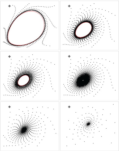For $b<b_0$ close to $b_0$ the closed invariant curve Γ is homeomorphic to a circle, and the restriction of the map to Γ is conjugated with a rotation on the circle. Thus, the dynamics on Γ are either periodic or quasi-periodic, depending on the rotation number. In Figure 1, we present the orbits and bifurcation closed invariant curve for some particular values of parameters.

Figure 1. Trajectories (black) and approximated invariant curve (red) for a = 0.5, m = 1.5, c = 1.0, $b_0=1.5$ and b = 1.45, b = 1.49 b = 1.495, b = 1.5, b = 1.53, b = 1.7, respectively for $\left(S\right)$ model.

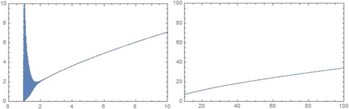
Figure 2. Bifurcation diagrams in b−P plane for a = 0.5, c = 1.0, and m = 1.5 for $\left(S\right)$ model.

Biologically, it means that if there exists cooperative hunting between parasitoids (m>1), and the intrinsic growth rate of the host population that are not safe from attack by parasitoids b is smaller than critical value $b_0>0$, then the host and parasitoid density will likely be quasi-periodic over time, and if that intrinsic growth is greater than the critical value $b_0$, both populations are in the coexisting steady state.

5.2. Hassel-Varley model $\left(HV\right)$

In this section, we study the effect of the presence of a spatial refuge on the stability and bifurcation of generalization of the Nicholson–Bailey model, proposed by Hassel and Valrey, see [9]: (13) $\begin{array}{rl}{H}_{n+1}& =a{H}_n+b{H}_n{\mathrm{e}}^{-P_n^m}\\ P_{n+1}& =c{H}_n(1-{\mathrm{e}}^{-P_n^m})\end{array},0<m\le 1.$(13) for $f\left(y\right)={\mathrm{e}}^{-y^m}$, $0<m\le 1$, proposed by Hassell and Varley (1969) [9]. One can see $f^{\prime }\left(y\right)=-m{\mathrm{e}}^{-y^m}{y}^{m-1}<0,f\left(0\right)=1\mathrm{a}\mathrm{n}\mathrm{d}f\left(\mathrm{\infty }\right)=0.$ Also, (14) $\begin{array}{rl}{f}^{″}\left(y\right)& =m^2{\mathrm{e}}^{-y^m}{y}^{2m-2}+(1-m)m{\mathrm{e}}^{-y^m}{y}^{m-2}>0\\ f^{‴}\left(y\right)& =-{\mathrm{e}}^{-y^m}\left(m^3{y}^{3m-3}+(1-m)m^2{y}^{2m-3}+m^2(2-2m)y^{2m-3}\right.\\ & \left.+(2-m)(1-m)m{y}^{m-3}\right)<0.\end{array}$(14) The non-trivial equilibrium $(H^{\ast },P^{\ast })=\left(\frac{b{\left(\ln \left({\displaystyle \frac{b}{1-a}}\right)\right)}^{\frac{1}{m}}}{c(a+b-1)},{\left(\ln \left(\frac{b}{1-a}\right)\right)}^{\frac{1}{m}}\right)$ exists for 1−b<a<1 and b>0. In Figure 3, we present the bifurcation diagrams in b−y plane.

Figure 3. Bifurcation diagrams in b−P plane for a = 0.1, c = 1.0. and m = 0.4 for $\left(HV\right)$ model.

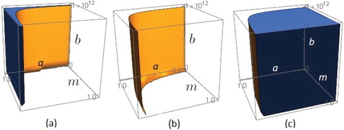
The Neimark–Sacker border surface (see Figure 4) $P^{\ast }{f}^{\prime }\left(P^{\ast }\right)=\frac{1-a-b}{b(a+b)}$, which separates region of stability and instability, is given by $\ln \left(\frac{b}{1-a}\right)=\frac{a+b-1}{(1-a)m(a+b)}$.

Figure 4. The corresponding regions of (a) stability (b) Hopf border surface and (c) instability in a−m−b space for $\left(HV\right)$.

The following Corollary, which follows directly from Lemma 3.2, shows that the refuge can have a local stabilizing effect:

Corollary 5.2

Assume a + b>1 and $0\le a<1$. Then the equilibrium point $(H^{\ast },P^{\ast })$ is

1. locally asymptotically stable if $\ln \left(\frac{b}{1-a}\right)<\frac{a+b-1}{(1-a)m(a+b)}.$

2. a repeller if and only if $\ln \left(\frac{b}{1-a}\right)>\frac{a+b-1}{(1-a)m(a+b)}.$

3. a non-hyperbolic equilibrium if and only if $\ln \left(\frac{b}{1-a}\right)=\frac{a+b-1}{(1-a)m(a+b)}.$

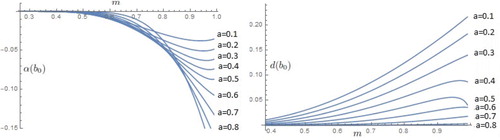
In Figure 5, we present the graphs of the functions $\alpha \left(b_0\right)\left(m\right)$ and $d\left(b_0\right)\left(m\right)$ for some values of a.

Figure 5. Graphs of the functions $\alpha \left(b_0\right)\left(m\right)$ and $d\left(b_0\right)\left(m\right)$ for some values of a for $\left(HV\right)$ model.

Let $b_0$ be solution of equation $\ln \left(\frac{b}{1-a}\right)=\frac{a+b-1}{(1-a)m(a+b)}$ such that $a+b_0>1$. By using the fact $\ln \left(\frac{b_0}{1-a}\right)=\frac{a+b_0-1}{(1-a)m(a+b_0)},$ we obtain $f^{″}\left(P^{\ast }\right)=\frac{m\left((a-1)m\left(a+b_0\right)-a\left(a+b_0-2\right)+2b_0-1\right)}{b_0\left(a+b_0\right)\left({\displaystyle \frac{a+b_0-1}{(1-a)m\left(a+b_0\right)}}\right){}^{\frac{2-m}{m}}}>0$ and $f^{‴}\left(P^{\ast }\right)=-\frac{(1-a)m(a+b_0-1)\mathrm{\Psi }}{b_0(a+b_0-1){\left({\displaystyle \frac{a+b_0-1}{(1-a)m(a+b_0)}}\right)}^{\frac{3-m}{m}}}<0,$ where $\mathrm{\Psi }=\frac{3m(a+b-1)}{(a-1)(a+b_0)}+\frac{(a+b_0-1{)}^2}{(a-1{)}^2(a+b_0{)}^2}-\frac{3(a+b_0-1)}{(a-1)(a+b_0)}+m^2-3m+2.$ By using this, we have $d\left(b_0\right)={\left.\frac{d|\mu \left(b\right)|}{db}\right|}_{b=b_0}=\frac{(1-a)m(a+b_0{)}^2-b_0}{2b_0(a+b_0-1)(a+b_0)}.$ and $\alpha \left(b_0\right)=-\frac{\begin{array}{c}\left((a-1{)}^2{m}^2\left(a+b_0\right){}^2-(1-a)am\left(a+b_0-1\right)\left(a+b_0\right)\right.\\ \left.+b_0\left(a\left(a+b_0\right)-1\right)\right)\end{array}}{4\left(\frac{a+b_0-1}{(1-a)m\left(a+b_0\right)}\right){}^{\frac{2}{m}}(a-1{)}^2\left(a+b_0\right){}^2}.$ By using numerical calculations, we obtain that $\alpha \left(b_0\right)<0$ and $d\left(b_0\right)>0$, for $0<m\le 1$, and $1-b_0<a<1$, see Table 1. By Theorem 4.2, an unique and stable invariant curve Γ bifurcates from the coexistence fixed point ($b<b_0)$ when the parameter b crosses the bifurcation value $b_0$ (supercritical Neimark–Sacker bifurcation). At $b=b_0$, the fixed point becomes an unstable focus and for $b>b_0$ an attracting closed curve Γ exists, surrounding the unstable fixed point. All orbits starting outside or inside the closed invariant curve, except at the origin, tend to the attracting closed curve. For b close to $b_0$, the closed invariant curve Γ is homeomorphic to a circle, and the restriction of the map to Γ is conjugated with a rotation on the circle. Thus, the dynamics on Γ are either periodic or quasi-periodic, depending on the rotation number. In Figure 6, we present the orbits and approximated bifurcation closed invariant curve for some particular values of parameters.

Figure 6. Trajectories (black) and approximated invariant curve (red) for a = 0.1, m = 0.4, c = 1.0, $b_0\approx 11.358951291565068$ and b = 11.239, b = 11.349 $b=b_0$, b = 11.36, b = 11.37, b = 11.48, respectively, for $\left(HV\right)$.

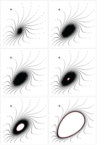
Table 1. The coefficients $b_0$, $d\left(b_0\right)$, and $\alpha \left(b_0\right)$ for some values of a, m and c = 1.

a	m	$b_0$	$d\left(b_0\right)$	$\alpha \left(b_0\right)$
0.2	0.2	408.115	0.000193498	$-8.41286\times {10}^{-10}$
0.3	0.2	878.357	0.0000791367	$-4.12591\times {10}^{-10}$
$0.4$	$0.2$	$2487.81$	$0.0000240465$	$-1.57987\times {10}^{-10}$
$0.2$	$0.3$	$47.2634$	$0.00236688$	$-6.27282\times {10}^{-6}$
$0.3$	$0.3$	$76.9854$	$0.00129697$	$-4.51672\times {10}^{-6}$
$0.4$	$0.3$	$149.558$	$0.00058343$	$-2.78057\times {10}^{-6}$
$0.5$	$0.3$	$386.17$	$0.000191366$	$-1.45415\times {10}^{-6}$
0.6	$0.3$	$1655.75$	$0.0000360768$	$-6.17268\times {10}^{-7}$
0.7	$0.3$	20062.	$2.24191\times {10}^{-6}$	$-1.91295\times {10}^{-7}$
0.8	$0.3$	$3.46154\times {10}^6$	$8.66663\times {10}^{-9}$	$-3.37687\times {10}^{-8}$
0.2	$0.4$	$14.7794$	0.00921253	$-0.000322423$
0.3	$0.4$	$21.0644$	0.00582341	$-0.000276712$
0.4	$0.4$	$34.3241$	0.00317278	$-0.000212010$
0.5	$0.4$	$69.0598$	0.0013643	$-0.000145720$
0.6	$0.4$	$200.876$	$0.000387863$	$-0.0000879042$
0.7	$0.4$	$1239.72$	$0.0000481118$	$-0.0000436707$
0.8	$0.4$	53655.	$7.45345\times {10}^{-7}$	$-0.0000152052$
0.2	$0.5$	$6.82909$	0.0223457	$-0.00272459$
0.3	$0.5$	$8.94916$	0.0153722	$-0.00259559$
0.4	$0.5$	$13.1514$	0.00937468	$-0.00225813$
0.5	$0.5$	$23.0316$	0.00472516	$-0.00181520$
0.6	$0.5$	$54.1873$	$0.00171009$	$-0.00133904$
0.7	$0.5$	$228.988$	0.000319442	$-0.000875038$
0.8	$0.5$	$4395.28$	0.0000113525	$-0.000456443$
0.2	$0.6$	$3.83278$	0.0423834	$-0.00984863$
0.3	$0.6$	$4.70446$	0.0308358	$-0.0101025$
0.4	$0.6$	$6.42245$	0.0202532	$-0.00958838$
0.5	$0.6$	$10.2912$	0.0113319	$-0.00855720$
0.6	$0.6$	$21.3369$	$0.00480405$	$-0.00720453$
0.7	$0.6$	$71.8832$	0.00117329	$-0.00563043$
0.8	$0.6$	$823.685$	0.0000721954	$-0.00383243$
0.2	$0.7$	$2.40189$	0.0693849	$-0.0221926$
0.3	$0.7$	$2.77369$	0.0524804	$-0.0241553$
0.4	$0.7$	$3.55315$	0.0362865	$-0.0245286$
0.5	$0.7$	$5.33549$	0.0218627	$-0.0236906$
0.6	$0.7$	$10.2306$	0.0103803	$-0.0220000$
0.7	$0.7$	$30.0575$	0.00306441	$-0.0195813$
0.8	$0.7$	$245.784$	0.000277706	$-0.0161163$
0.2	$0.8$	$1.60905$	$0.103068$	$-0.0369197$
0.3	$0.8$	$1.73865$	0.0799625	$-0.0423442$
0.4	$0.8$	$2.08061$	0.0571231	$-0.0455823$
0.5	$0.8$	$2.95318$	0.0363071	$-0.0470695$
0.6	$0.8$	$5.41502$	0.018864	$-0.0474562$
0.7	$0.8$	$14.7851$	0.00644749	$-0.0469722$
0.8	$0.8$	$97.2016$	0.000778919	$-0.0447984$

Note that the direction of supercritical Neimark–Sacker bifurcation in $\left(HV\right)$ is the opposite of the model $\left(S\right)$.

5.3. The parasitoid–parasitoid interaction model $\left(PP\right)$

In this section, we study the stability and bifurcation of model $\left(PP\right)$, if a spatial refuge is present: (15) $\begin{array}{rl}{H}_{n+1}& =a{H}_n+b{H}_n{\mathrm{e}}^{-\frac{\sqrt{1+P_n}-1}{m}}\\ P_{n+1}& =c{H}_n\left(1-{\mathrm{e}}^{-\frac{\sqrt{1+P_n}-1}{m}}\right)\end{array},m>0$(15) for $f\left(y\right)={\mathrm{e}}^{-\frac{\sqrt{1+y}-1}{m}}$, m>0. One can see $f^{\prime }\left(y\right)=-\frac{{\mathrm{e}}^{\frac{1-\sqrt{y+1}}{m}}}{2m\sqrt{y+1}}<0$, $f\left(0\right)=1$ and $f\left(\mathrm{\infty }\right)=0$. The non-trivial equilibrium $\begin{array}{rl}& (H^{\ast },P^{\ast })\\ & =\left(\frac{bm\ln \left({\displaystyle \frac{b}{1-a}}\right)\left(m\ln \left({\displaystyle \frac{b}{1-a}}\right)+2\right)}{c(a+b-1)},m\ln \left(\frac{b}{1-a}\right)\left(m\ln \left(\frac{b}{1-a}\right)+2\right)\right)\end{array}$ exists for 1−b<a<1 and b>0.

The Neimark–Sacker border surface (see Figure 7) $P^{\ast }{f}^{\prime }\left(P^{\ast }\right)=\frac{1-a-b}{b(a+b)}$, which separated region of stability and instability, is given by $\begin{array}{rl}& \ln \left(\frac{b}{1-a}\right)\\ & =\frac{m(a+b)+a(a+b-1)-b-m+\sqrt{m^2(a+b-1{)}^2+(a-1{)}^2(a+b{)}^2}}{(1-a)m(a+b)}.\end{array}$The following Corollary, which follows directly from Lemma 3.2, shows that the refuge can have a local stabilizing effect:

Corollary 5.3

Assume a + b>1 and $0\le a<1$. Then, the equilibrium point $(H^{\ast },P^{\ast })$ is

1. locally asymptotically stable if $\begin{array}{rl}& \ln \left(\frac{b}{1-a}\right)\\ & <\frac{m(a+b)+a(a+b-1)-b-m+\sqrt{m^2(a+b-1{)}^2+(a-1{)}^2(a+b{)}^2}}{(1-a)m(a+b)}.\end{array}$

2. a repeller if and only if $\begin{array}{rl}& \ln \left(\frac{b}{1-a}\right)\\ & >\frac{m(a+b)+a(a+b-1)-b-m+\sqrt{m^2(a+b-1{)}^2+(a-1{)}^2(a+b{)}^2}}{(1-a)m(a+b)}.\end{array}$

3. a non-hyperbolic equilibrium if and only if $\begin{array}{rl}& \ln \left(\frac{b}{1-a}\right)\\ & =\frac{m(a+b)+a(a+b-1)-b-m+\sqrt{m^2(a+b-1{)}^2+(a-1{)}^2(a+b{)}^2}}{(1-a)m(a+b)}.\end{array}$

Figure 7. The corresponding regions of (a) stability (b) Hopf border surface and (c) instability in a−m−b space for $\left(PP\right)$ model.

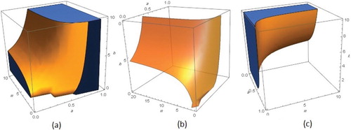
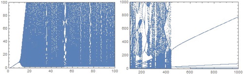
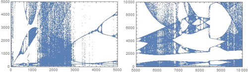
Figure 8. Bifurcation diagrams in b−P plane for a = 0.01, c = 1.0. and $m_0=6.040735644332293$ for $\left(PP\right)$ model.

Let $b_0$ be solution of equation $\begin{array}{rl}& \ln \left(\frac{b_0}{1-a}\right)\\ & =\frac{m(a+b_0)+a(a+b_0-1)-b_0-m+\sqrt{m^2(a+b_0-1{)}^2+(a-1{)}^2(a+b_0{)}^2}}{(1-a)m(a+b_0)},\end{array}$ such that $a+b_0>1$. Let $\mathrm{\Lambda }=\sqrt{m^2(a+b_0-1{)}^2+(a-1{)}^2(a+b_0{)}^2}.$ We obtain $\begin{array}{rl}{f}^{″}\left(P^{\ast }\right)& =\frac{(1-a)\left(m\log \left(\frac{b_0}{1-a}\right)+m+1\right)}{4b_0{m}^2\left(m\log \left(\frac{b_0}{1-a}\right)+1\right){}^3}\\ & =\frac{(a-1{)}^3(a+b_0{)}^2\left(m\left((a-2)b_0+(a-1{)}^2\right)-\mathrm{\Lambda }\right)}{4b{m}^2\left(m\right(a+b_0-1)+\mathrm{\Lambda }{)}^3}\\ f^{‴}\left(P^{\ast }\right)& =\frac{(a-1)\left(m\log \left(\frac{b_0}{1-a}\right)\left(m\log \left(\frac{b_0}{1-a}\right)+3m+2\right)+3m(m+1)+1\right)}{8b_0{m}^3\left(m\log \left(\frac{b_0}{1-a}\right)+1\right){}^5}=\\ & =-\frac{(a-1{)}^4\left(a+b_0\right){}^4\left(m^2\left(a\left(3a\left(a+b_0-3\right)-9b_0+11\right)+8b_0-7\right)\right)}{8b_0{m}^3\left(m\left(a+b_0-1\right)-\mathrm{\Lambda }\right){}^5}\\ & -\frac{\begin{array}{c}(a-1{)}^4\left(a+b_0\right){}^3\\ \left((a-1{)}^2\left(a+b_0\right)+\mathrm{\Lambda }m\left(a\left(3a+3b_0-5\right)-5b_0+2\right)+2m^2\right)\end{array}}{8b_0{m}^3\left(m\left(a+b_0-1\right)-\mathrm{\Lambda }\right){}^5}\end{array}$ By using this, we have $\begin{array}{rl}d\left(b_0\right)& =\frac{a^3+a^2(b-1)+a\left(m^2-2b\right)+b\left(m^2+1\right)-m(\mathrm{\Lambda }+m)}{2(1-a)b(a+b)}\\ \alpha \left(b_0\right)& =-\frac{b_0{\left(P^{\ast }\right)}^2(a+b_0)\mathrm{\Gamma }+2(a+b_0-1{)}^3}{4{\left(P^{\ast }\right)}^2(a+b_0-1{)}^2(a+b_0)},\end{array}$ where $\begin{array}{rl}\mathrm{\Gamma }& =P^{\ast }\left(a+b_0-1\right)\left(a+b_0\right)f^{\left(3\right)}\left(P^{\ast }\right)+2b_0{\left(P^{\ast }\right)}^2\left(a+b_0\right){}^2{f}^{″}{\left(P^{\ast }\right)}^2\\ & -\left(a+b_0-1\right)\left(2a+2b_0-1\right)f^{″}\left(P^{\ast }\right).\end{array}$

By numerical calculations, we obtain that $d\left(b_0\right)>0$ for m>0, and $1-b_0<a<1$, see Table 2. It appears that $\alpha \left(b_0\right)$ changes its sign, which implies the presence of the so-called Chenciner bifurcation. This means that we have supercritical and subcritical Neimark–Sacker bifurcation. If $\alpha \left(b_0\right)<0$, then the behaviour of the model is the same as in model $\left(HV\right)$. A typical case is illustrated in Figures 9 and 10. If $\alpha \left(b_0\right)>0$, then by Theorem 4.2, a repelling closed invariant curve exists surrounding the stable fixed point, for $b<b_0$ as b increases the repelling closed curve decreases in size and merging with the fixed point at $b=b_0;$ leaving a repelling focus (subcritical Neimark–Sacker bifurcation). In this case, closed repelling curve is generally the boundary of the basin of attraction of the stable fixed point. Figure 11 shows the typical behaviour of the solutions of the model $\left(PP\right)$ if $d\left(b_0\right)>0$ and $\alpha \left(b_0\right)>0$.

Figure 9. Supercritical Hopf bifurcation for a = 0.01, m = 10, c = 1 where $b_0\approx 4.213439215488374$, $d\left(b_0\right)\approx 0.040557714674268774$, and $\alpha \left(b_0\right)\approx -8.53863\times {10}^{-7}$. Trajectories (orange, blue and black) and approximated attractive invariant curve (red) for (a) b = 4.2 (b) b = 4.214 (c) b = 4.22 and (d) b = 4.225. For $\left(PP\right)$ model.

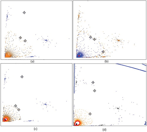
Figure 10. Supercritical Hopf bifurcation for a = 0.1, m = 10, c = 1 where $b_0\approx 4.803161528187171$, $d\left(b_0\right)\approx 0.03290632603362123$, and $\alpha \left(b_0\right)\approx -2.10776\times {10}^{-7}$. Trajectories (orange, blue and black) and approximated attractive invariant curve (red) for (c) b = 4.81 and (d) b = 4.88 and trajectories for (a) b = 4.6 and (b) b = 4.8. For$\left(PP\right)$ model.

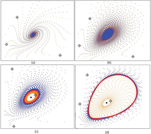
Figure 11. Subcritical Hopf bifurcation for a = 0.1, m = 1.8, c = 1 where $b_0\approx 2.381196753601008$, $d\left(b_0\right)\approx 0.043144048585692873$, and $\alpha \left(b_0\right)\approx 0.00010912518875029679$. Trajectories (orange, blue and black) and approximated repelling invariant curve (red) for (a) b = 2.37 and (b) b = 2.38 and trajectories for (c) b = 2.382 and (b) b = 2.39. For $\left(PP\right)$ model.

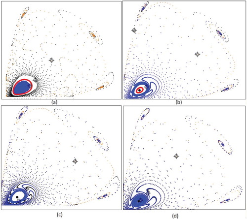
Table 2. The coefficients $b_0$, $d\left(b_0\right)$, and $\alpha \left(b_0\right)$ for some values of a, m and c = 1.

a	m	$b_0$	$d\left(b_0\right)$	$\alpha \left(b_0\right)$
0.01	$1.1$	$1.16932$	$0.0221388$	$0.0191121$
0.01	$2.1$	$2.28577$	0.0489982	$0.000334622$
0.01	$3.1$	$2.92481$	$0.0470603$	$0.000029227$
0.01	$4.1$	$3.32418$	$0.0450936$	$4.31592\times {10}^{-6}$
0.01	5.1	$3.59515$	$0.0436907$	$6.6182\times {10}^{-7}$
0.01	$6.1$	$3.79047$	0.0426817	$-1.63676\times {10}^{-8}$
0.05	$1.1$	$1.27047$	$0.0309502$	0.010163
0.05	$2.1$	$2.44035$	$0.0462047$	$0.000160244$
0.05	$3.1$	3.10621	$0.0435757$	$8.35346\times {10}^{-6}$
0.05	$4.1$	$3.52148$	0.0415353	$-6.04233\times {10}^{-7}$
0.05	$5.1$	$3.80292$	0.040149	$-9.90726\times {10}^{-7}$
0.05	$6.1$	$4.00566$	0.0391716	$-7.0604\times {10}^{-7}$
0.1	$1.1$	$1.42955$	$0.0369549$	0.00394312
0.1	$2.1$	$2.6814$	$0.0421882$	$0.0000197167$
0.1	$3.1$	3.38858	$0.039053$	$-9.10164\times {10}^{-6}$
0.1	$4.1$	$3.82837$	0.0370162	$-4.78208\times {10}^{-6}$
0.1	$5.1$	$4.12599$	0.0356905	$-2.40488\times {10}^{-6}$
0.1	$6.1$	$4.34019$	0.0347731	$-1.29881\times {10}^{-6}$
0.15	$1.1$	$1.63731$	$0.038771$	0.000786658
0.15	$2.1$	$2.99319$	$0.0377399$	$-0.0000623552$
0.15	3.1	$3.75297$	$0.0344211$	$-0.0000196141$
0.15	$4.1$	$4.22403$	0.0324749	$-7.32143\times {10}^{-6}$
0.15	$5.1$	$4.5423$	0.0312456	$-3.26624\times {10}^{-6}$
0.15	$6.1$	$4.77114$	0.0304067	$-1.65959\times {10}^{-6}$

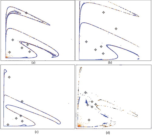
If $\alpha \left(b_0\right)=0$, then according to the theory, if $b<b_0$, then a repelling closed invariant curve exists surrounding the stable fixed point. All orbits starting inside the closed invariant curve tend to the stable fixed point. In this case, closed repelling curve is generally the boundary of the basin of attraction of the stable fixed point. If $b>b_0$, where b close to $b_0$, we may expect one (inner) or two (inner and outer) invariant curves. The inner curve is attracting, and it is either densely filled by successive iteration points, or it contains a periodic cycle with rotation number close to 1:7. The outer curve is repelling and separates the bounded orbits from the unbounded ones or orbits that converge to some periodic solution. For example, for a = 0.01, at $b_0\approx 3.780433954506987$, $m_0\approx 6.040735644332293$ we have $\alpha (b_0,m_0)\approx 0$, and Chenciner bifurcation occurs, see Figure 12. Bifurcation diagram is given by Figure 8.

Figure 12. Trajectories (orange, blue and black) for a = 0.01, $b_0\approx 3.780433954506987$, c = 1 where $m_0\approx 6.040735644332293$, and $\alpha \left(b_0\right)\approx 0$ for (a) b = 3.25, $m=m_0$ (b) b = 3.87, $m=m_0$ (c) $b=b_0$, m = 3.72 and (d) $b=b_0$, m = 8.97. for $\left(PP\right)$ model.

6. Conclusion

In this paper, we investigated the stability of a class of a host–parasitoid model with refuge. We found the conditions for the existence of equilibrium points. Also, we obtained results on stability of extinction, exclusion and coexistence equilibrium points. The both, hosts and parasitoids can coexist if the intrinsic growth rate of the host is grater than one. However, the parasitoid population will drive the host population to extinction if the intrinsic growth rate of the host is smaller than one. The parasitoid population becomes extinct if the growth rate is equal one.

We studied the existence of Neimark–Sacker bifurcation, by using b as the bifurcation parameter, for the unique positive equilibrium and compute asymptotic approximation of the invariant curve near the positive equilibrium point of System (1(1) $\begin{array}{rl}{H}_{n+1}& =a{H}_n+b{H}_{n}f\left(P_n\right)\\ P_{n+1}& =c{H}_n(1-f(P_n\left)\right),\end{array}$(1) ), according to the procedure given in [22]. We show that the model can undergo subcritical or/and supercritical Neimark–Sacker bifurcation. In the former situation, the parameter b can act as both a destabilizing and a stabilizing mechanism. The Neimark–Sacker bifurcation is highly relevant to the modelling of biological systems. In terms of the latter, the existence of a Neimark–Sacker bifurcation implies that both the host and parasitoids populations can oscillate around some mean values, and that these oscillations are stable and will continue indefinitely under suitable conditions. We applied and verified obtained results to the well known host–parasitoid models: $\left(S\right)$, $\left(HV\right)$ and $\left(PP\right)$. All tedious symbolic computation have been done with package Mathematica. We also use package Mathematica to produce all figures in this paper. The bifurcation diagrams clearly demonstrate our theoretical results by series of numerical computations, which have been done in package Mathematica.

In $\left(S\right)$ model if there exists cooperative hunting between parasitoids (m>1), and if $b<b_0$ an attracting closed curve exists, surrounding the unstable fixed point, when the parameter b crosses the bifurcation value $b_0$ (supercritical Neimark–Sacker bifurcation). As b increases, the attracting closed curve decreases in size and merging with the fixed point at $b=b_0$, leaving a stable fixed point (subcritical Neimark–Sacker bifurcation, see Figure 2). All orbits starting outside or inside the closed invariant curve, except at the origin, tend to the attracting closed curve. In Figure 1, we present the orbits and bifurcation closed invariant curve for some particular values of parameters. Biologically, it means that if the intrinsic growth rate of the host population that are not safe from attack by parasitoids b is smaller than critical value $b_0$, then the host and parasitoid density will likely be quasi-periodic over time, and if the intrinsic growth is greater than the critical value $b_0$, both populations are in the coexisting steady state.

In $\left(HV\right)$ model, an unique and stable invariant curve bifurcates from the coexistence fixed point ($b<b_0)$, when the parameter b crosses the bifurcation value $b_0$ (supercritical Neimark–Sacker bifurcation). At $b=b_0$, the fixed point becomes an unstable focus and for $b>b_0$ an attracting closed curve exists, surrounding the unstable fixed point. For b close to $b_0$, the closed invariant curve is homeomorphic to a circle, and the restriction of the map to this curve is conjugated with a rotation on the circle. In Figure 6, we present the orbits and approximated bifurcation closed invariant curve for some particular values of parameters. Note that the direction of supercritical Neimark–Sacker bifurcation in $\left(HV\right)$ is the opposite of the model $\left(S\right)$. Biologically, it means that if the intrinsic growth rate of the host population that are not safe from attack by parasitoids b is smaller than critical value $b_0$, both populations are in the coexisting steady state, and if the intrinsic growth is greater than the critical value $b_0$, host and parasitoid density will likely be oscillatory over time.

In $\left(PP\right)$ model, see Table 2, we see that there are positive and negative values of $\alpha \left(b_0\right)$. If $\alpha \left(b_0\right)<0$, then the behaviour of the model is the same as in model $\left(HV\right)$. A typical case is illustrated in Figures 9 and 11. If $\alpha \left(b_0\right)>0$, then by Theorem 4.2, a repelling closed invariant curve exists surrounding the stable fixed point, for $b<b_0$ as b increases the repelling closed curve decreases in size and merging with the fixed point at $b=b_0$; leaving a repelling focus (subcritical Neimark–Sacker bifurcation). As we have seen, for a = 0.01, c = 1.0 at $b_0\approx 3.780433954506987$, $m_0\approx 6.040735644332293$ we have $\alpha (b_0,m_0)=0$, which implies the presence of so-called Chenciner bifurcation, see Figure 12, i.e. Neimark–Sacker bifurcations which switch from being subcritical to being supercritical (see Figures 9 and 10), or vice versa, see [4]. Both stable equilibrium and stable circle are always surrounded by an unstable invariant circle bounding their basins of attraction. Biologically, it means that if the host and parasitoids density close to the equilibrium point, i.e. inside the repelling invariant curve, both populations are in the coexisting steady state. If we start too far away from the equilibrium point, we see ever increasing oscillations just as in the Nicholson–Baily model. When m goes to the infinity, $\left(PP\right)$ model goes to the $\left(HV\right)$ model, the stable circle grows large and large and it appears as if, in the limit, the circle disappears by moving off towards infinity or merging with the axes (see [17]).

It is clear, therefore, that the ability of a host to escape to a refuge can have a crucial impact on the stability of a host–parasitoid interaction, by damping irregular oscillations. For each of these models (S), (HV) and (PP), the corresponding regions of stability show that as parameter a gets closer to one, that is, as rate of escaping of a host population increases and approaches to one, then host–parasitiod interaction may lead to stability. A small rate of escaping of a host may lead to instability, regardless the rate of the interference m between the parasitoids. Also, we have noticed that increase in value of the parameter b may lead to stability of $\left(S\right)$ model, while this increase in value may lead to instability of $\left(HV\right)$ and $\left(PP\right)$ models.

Disclosure statement

No potential conflict of interest was reported by the authors.

References

- T. Agarwal, Bifurcation analysis of a host–parasitoid model with the beddington-deangelis functional response, Global J. Math. Anal. 2(2) (2014), pp. 565–569.
- V.A. Bailey and J. Nicholson, The balance of animal populations, Proc. Zool. Soc. Lond. 3 (1935), pp. 551–598.
- J. Banasiak, Notes on Mathematical Models in Biology, Lecture notes.
- A. Chenciner, Bifurcations de difféomorphisms de R2 au voisinage d'un point fixe ellyptique, in Les Houches Ecole d'Eté de Physique Théorique, G. Iooss and H.G. Helleman, eds., North Holland, Amsterdam, 1983, 273–348.
- P.L. Chesson and W.W. Murdoch, Aggregation of risk: Relationships among host–parasitoid models, Amer. Naturalist 127(5) (1986), pp. 696–715.
- Y. Chow and S. Jang, Neimark–Sacker bifurcations in a host–parasitoid system with a host refuge, Disc. Cont. Dyn. Sys., Ser. B 21 (2016), pp. 1713–1728.
- M.P. Hassell, The Dynamics of Arthropod Predator–Prey Systems, Princeton Univeristy Press, Princeton, NJ, 1978.
- M.P. Hasell, Parasitism in patchy environments, IMA J. Math. Appl. Med. Biol. 1 (1984), pp. 123–133.
- M.P. Hasell and G.C. Varley, New inductive population model for insect parasites and its bearing on biological control, Nature 223 (1969), pp. 1133–1137.
- M.P. Hassell and D.J. Rogers, Insect parasite responses in the development of population models, J. Animal Ecol. 41 (1971), pp. 661–676.
- W.T. Jamieson, On the global behaviour of May's host–parasitoid model, J. Differ. Equ. Appl. 25 (2019), pp. 583–596.
- S. Jang, Alle effects in a disrete-time host–parasitoid model, J. Differ. Equ. Appl. 12 (2006), pp. 165–181.
- S. Jang, Discrete-time host–parasitoid models with Alle effect: Density dependence vs. parasitism, J. Differ. Equ. Appl. 17 (2011), pp. 525–539.
- S. Kapçak, U. Ufuktepe, and S. Elaydi, Stability and invariant manifolds of a generalized Beddington host–parasitoid model, J. Biol. Dyn. 7(1) (2013), pp. 233–253.
- S. Kapçak, U. Ufuktepe, and S. Elaydi, Stability of a predator–prey model with refuge effect, J. Differ. Equ. Appl. 22(7) (2016), pp. 989–1004, doi:10.1080/10236198.2016.1170823.
- G. Ladas, G. Tzanetopoulos, and A. Tovbis, On May's host parasitoid model, J. Differ. Equ. Appl.2(2) (1996), pp. 195–204, 101, 1996.
- H.A. Lauwerier and J.A. Metz, Hopf bifurcation in host–parasitoid models, IMA J. Math. Appl. Med. Biol. 3 (1986), pp. 191–210.
- X. Liu, Y. Chu, and Y. Liu, Bifurcation and chaos in a host–parasitoid model with a lower bound for the host. Adv. Differ. Equ. 2018 (2018), p. 31.
- G. Livadiotis, L. Assas, B. Dennis, S. Elaydi, and E. Kwesi, A discrete time host–parasitoid model with Alle effect, J. Biol. Dyn. 9 (2015), pp. 34–51.
- R.M. May, Density dependence in host–parasitoid models, J. Animal Ecol. 50 (1981), pp. 855–865.
- R.M. May, Host–parasitoid systems in patchy environments: A phenomenological model, J. Animal Ecol. 47 (2015), pp. 833–844.
- K. Murakami, The invariant curve caused by Neimark–Sacker bifurcation, Dyn. Cont. Discrete Impulsive Syst. 9(1) (2002), pp. 121–132.
- D. Qamar and M. Hussain, Controlling chaos and Neimark–Sacker bifurcation in a host–parasitoid model, Asian J. Control 21(4) (2019), pp. 1–14.
- D. Qamar and U. Saeed, Bifurcation analysis and chaos control ina host–parasitoid model, Math. Methods Appl. Sci. 40 (2017), doi:10.1002/mma.4395.
- D.J. Rogers, Random search and insect population models, J. Animal Ecol. 41 (1972), pp. 369–383.
- D.J. Rogers and M.P. Hassell, General models for insect parasite and predator searching behaviour: Interference, J. Animal Ecol. 43 (1974), pp. 239–253.
- S.J. Schreiber, Host–parasitoid dynamics of a generalized Thompson model, J. Math. Biol. 52 (2006), pp. 719–732.
- S. Tang and L. Chen, Chaos in functional response host–parasitoid ecosystem models, Chaos Solitons Fractals 39 (2009), pp. 1259–1269.
- W. Thompson, On the effect of randoma oviposition on the action of entomophagous parasities as agents of natural control, Parasitology 21 (1929), pp. 180–188.
- M. Vaz Nunez, Limietcycli in Het Parasitoid-Gastheer Model van Hassell–Varley en een Modificatie Daarvan, Institute of Theoretical Biology, Leiden, 1977, Internal report.
- S. Wiggins, Introduction to Applied Nonlinear Dynamical Systems and Chaos, 2nd ed., Texts in Applied Mathematics, Vol. 2, Springer-Verlag, New York, 2003.
- D. Wu and H. Zhao, Global qualitative analysis of a discrete host–parasitoid model with refuge and strong Allee effects, Math. Methods Appl. Sci. 41 (2018), pp. 2039–2062, doi:10.1002/mma.4731.