Coinfection dynamics of heroin transmission and HIV infection in a single population

Abstract

We propose a model of a joint spread of heroin use and HIV infection. The unique disease-free equilibrium always exists and it is stable if the basic reproduction numbers of heroin use and HIV infection are both less than 1. The semi-trivial equilibrium of HIV infection (heroin use) exists if the basic reproduction number of HIV infection (heroin use) is larger than 1 and it is locally stable if and only if the invasion number of heroin use (HIV infection) is less than 1. When both semi-trivial equilibria lose their stability, a coexistence equilibrium occurs, which may not be unique. We compare the model to US data on heroin use and HIV transmission. We conclude that the two diseases in the US are in a coexistence regime. Elasticities of the invasion numbers suggest two foci for control measures: targeting the drug abuse epidemic and reducing HIV risk in drug-users.

Keywords:

• Coexistence
• Invasion numbers
• epidemic model
• heroin use
• HIV transmission

1. Introduction

Heroin users are at high risk for addiction and it is estimated that about 23% of individuals who use heroin become dependent on it. The study of modeling heroin addiction and spread in [6] shows that classical epidemic models can be used for modeling drug addiction and informing control policies. Since then the mathematical models have been widely used for modelling heroin abuse and transmission [4,7,8,13]. The opioid epidemic has been drawing much interest lately because of rapidly increasing number of users and deaths. Human immunodeficiency virus (HIV) can be transmitted sexually or through sharing of contaminated needles or syringes. HIV infection associated with injection drug use (IDU) and needle sharing has been on the rise in many countries, while injection of heroin drugs has become increasingly common among drug users. Thus the study of the coinfection of heroin and HIV transmission in a single population has very significant impact in epidemiology.

Coinfection epidemic models with multiple specific diseases, such as HIV/TB [19,21], HIV/gonorrhea [18], HIV/malaria [1,2], malaria and meningitis [14], or general diseases [3,12] show that disease co-circulation has major consequences for between host disease dynamics. Since coinfection leads to more complex dynamics in two disease epidemic models, one expects the presence of coexistence equilibria whose explicit expressions are difficult to obtain. Blyuss and Kyrychko [3] studied a susceptible-infectious-susceptible $\left(SIS\right)$ coinfection two-disease model, but an expression for the endemic steady-state with both diseases in the case of coinfection was not obtained analytically and only some numerical simulations of this steady-state were presented. Gao et al. studied a coinfection SIS epidemic model with bilinear incidence, and obtained through simulations richer dynamic behavior such as backward bifurcations and Hopf bifurcation [9].

Using invasion reproduction numbers (see [20]), Iannelli et al.) [11] strictly proved the existence and local stability of a coexistence equilibrium in an epidemic model with super-infection and perfect vaccination. After that, using the invasion reproduction numbers, Martcheva and Pilyugin [16] proved that there are two coexistence equilibria in a coinfection epidemic model of two diseases with time-since-infection structure. For more information about the invasion reproduction numbers, one can refer to [15–17] and references therein.

To account for the coinfection and co-transmission of heroin and HIV spreading through a single population, in this paper, we propose a new mathematical model with heroin & HIV coinfection. We use standard incidence terms to model the new cases in both diseases. In what follows, we divide the population into five classes, namely the number of susceptibles, $S\left(t\right)$, the number of heroin drug users, $U\left(t\right)$, the number of HIV-infected individuals, $V\left(t\right)$, the number of coinfected (heroin/HIV) individuals, $I\left(t\right)$, and the number of individuals with AIDS, $A\left(t\right)$. We assume that individuals with AIDS are isolated and that the total number of the population is N = S + U + V + I. The effective contact rate between the individuals with heroin addiction and the susceptibles is $C_1$ and the transmissibility of heroin drug use per effective contact is assumed to be ${\text{β}}_U$. Meanwhile, the effective contact rate between the HIV infected individuals and the susceptibles is $C_2$ and the infectivity of HIV infected individuals per effective contact is assumed to be ${\text{β}}_V$. Then we have the following force of infections ${\lambda }_U\left(t\right)$, ${\lambda }_V\left(t\right)$ of heroin and HIV spread in a single population, (1) $\begin{array}{rl}& {\lambda }_U\left(t\right)={\text{β}}_U{C}_1\frac{U\left(t\right)+I\left(t\right)}{N\left(t\right)}:={\text{β}}_1\frac{U\left(t\right)+I\left(t\right)}{N\left(t\right)},\\ & {\lambda }_V\left(t\right)={\text{β}}_V{C}_2\frac{V\left(t\right)+I\left(t\right)}{N\left(t\right)}:={\text{β}}_2\frac{V\left(t\right)+I\left(t\right)}{N\left(t\right)},\end{array}$(1) With the above notation of the force of infection, the model takes the form: (2) $\begin{array}{rl}& \frac{\mathrm{d}S\left(t\right)}{\mathrm{d}t}=\mathrm{\Lambda }-\mu S\left(t\right)+\delta U\left(t\right)-{\lambda }_U\left(t\right)S\left(t\right)-{\lambda }_V\left(t\right)S\left(t\right),\\ & \frac{\mathrm{d}U\left(t\right)}{\mathrm{d}t}={\lambda }_U\left(t\right)S\left(t\right)-q{\lambda }_V\left(t\right)U\left(t\right)-(\mu +d_U+\delta )U\left(t\right),\\ & \frac{\mathrm{d}V\left(t\right)}{\mathrm{d}t}={\lambda }_V\left(t\right)S\left(t\right)-{\lambda }_U\left(t\right)V\left(t\right)-(\mu +d_V+{\gamma }_1)V\left(t\right)+\sigma \delta I\left(t\right),\\ & \frac{\mathrm{d}I\left(t\right)}{\mathrm{d}t}=q{\lambda }_V\left(t\right)U\left(t\right)+{\lambda }_U\left(t\right)V\left(t\right)-(\mu +d_I+{\gamma }_2)I\left(t\right)-\sigma \delta I\left(t\right),\\ & \frac{\mathrm{d}A\left(t\right)}{\mathrm{d}t}={\gamma }_{1}V\left(t\right)+{\gamma }_{2}I\left(t\right)-(\mu +d_A)A\left(t\right),\end{array}$(2) with the initial conditions: (3) $S\left(0\right)=S_0,U\left(0\right)=U_0,V\left(0\right)=V_0,I\left(0\right)=I_0,A\left(0\right)=A_0.$(3) In system (2(2) $\begin{array}{rl}& \frac{\mathrm{d}S\left(t\right)}{\mathrm{d}t}=\mathrm{\Lambda }-\mu S\left(t\right)+\delta U\left(t\right)-{\lambda }_U\left(t\right)S\left(t\right)-{\lambda }_V\left(t\right)S\left(t\right),\\ & \frac{\mathrm{d}U\left(t\right)}{\mathrm{d}t}={\lambda }_U\left(t\right)S\left(t\right)-q{\lambda }_V\left(t\right)U\left(t\right)-(\mu +d_U+\delta )U\left(t\right),\\ & \frac{\mathrm{d}V\left(t\right)}{\mathrm{d}t}={\lambda }_V\left(t\right)S\left(t\right)-{\lambda }_U\left(t\right)V\left(t\right)-(\mu +d_V+{\gamma }_1)V\left(t\right)+\sigma \delta I\left(t\right),\\ & \frac{\mathrm{d}I\left(t\right)}{\mathrm{d}t}=q{\lambda }_V\left(t\right)U\left(t\right)+{\lambda }_U\left(t\right)V\left(t\right)-(\mu +d_I+{\gamma }_2)I\left(t\right)-\sigma \delta I\left(t\right),\\ & \frac{\mathrm{d}A\left(t\right)}{\mathrm{d}t}={\gamma }_{1}V\left(t\right)+{\gamma }_{2}I\left(t\right)-(\mu +d_A)A\left(t\right),\end{array}$(2) ), the parameter Λ is the recruitment rate, μ is the natural death rate, δ is the recovery rate of heroin users, ${\gamma }_1$ and ${\gamma }_2$ are the transition rates from HIV infection and coinfection to AIDS, respectively (${\gamma }_2\ge {\gamma }_1$), $d_U$ is the death rate induced by heroin addiction, $d_V$ is the death rate induced by HIV infection, $d_I$ is the death rate induced by coinfection with $d_I\ge d_V$, $d_A$ is the death rate induced by AIDS. The term $q{\lambda }_V$ denotes that the force of infection of a heroin user infected by HIV. The term $\sigma \delta I$ denotes the recovery rate of an individual from coinfection to HIV infection only. Moreover, we assume that at most one disease can be transmitted per contact with a coinfected individual.

To the best of our knowledge, there are no relevant research results on coinfection of heroin abuse and HIV infection. In this paper we employ operator theory and fixed point theorem to derive the existence of a coexistence equilibrium, which can overcome the difficulties created by the direct algebraic computations. The method of this paper can be extended to study the coinfection epidemic models with saturating incidences. The paper is organized as follows. In the next section, some preliminary results of system (2(2) $\begin{array}{rl}& \frac{\mathrm{d}S\left(t\right)}{\mathrm{d}t}=\mathrm{\Lambda }-\mu S\left(t\right)+\delta U\left(t\right)-{\lambda }_U\left(t\right)S\left(t\right)-{\lambda }_V\left(t\right)S\left(t\right),\\ & \frac{\mathrm{d}U\left(t\right)}{\mathrm{d}t}={\lambda }_U\left(t\right)S\left(t\right)-q{\lambda }_V\left(t\right)U\left(t\right)-(\mu +d_U+\delta )U\left(t\right),\\ & \frac{\mathrm{d}V\left(t\right)}{\mathrm{d}t}={\lambda }_V\left(t\right)S\left(t\right)-{\lambda }_U\left(t\right)V\left(t\right)-(\mu +d_V+{\gamma }_1)V\left(t\right)+\sigma \delta I\left(t\right),\\ & \frac{\mathrm{d}I\left(t\right)}{\mathrm{d}t}=q{\lambda }_V\left(t\right)U\left(t\right)+{\lambda }_U\left(t\right)V\left(t\right)-(\mu +d_I+{\gamma }_2)I\left(t\right)-\sigma \delta I\left(t\right),\\ & \frac{\mathrm{d}A\left(t\right)}{\mathrm{d}t}={\gamma }_{1}V\left(t\right)+{\gamma }_{2}I\left(t\right)-(\mu +d_A)A\left(t\right),\end{array}$(2) ) are presented, including the basic reproduction numbers, and the existence of equilibria. In Section 3, the local stability results of the disease-free equilibrium, the semi-trivial equilibrium of heroin transmission and the semi-trivial equilibrium of HIV infection are strictly proved, by use of the basic reproduction numbers and the invasion reproduction numbers. The existence of a coexistence equilibrium of heroin and HIV is obtained in Section 4. In Section 5 some numerical simulations are carried out to illustrate and extend the theoretical results. In Section 6 we summarize our conclusions.

2. Preliminary results

Since the first four equations are independent of the last equation of system (2(2) $\begin{array}{rl}& \frac{\mathrm{d}S\left(t\right)}{\mathrm{d}t}=\mathrm{\Lambda }-\mu S\left(t\right)+\delta U\left(t\right)-{\lambda }_U\left(t\right)S\left(t\right)-{\lambda }_V\left(t\right)S\left(t\right),\\ & \frac{\mathrm{d}U\left(t\right)}{\mathrm{d}t}={\lambda }_U\left(t\right)S\left(t\right)-q{\lambda }_V\left(t\right)U\left(t\right)-(\mu +d_U+\delta )U\left(t\right),\\ & \frac{\mathrm{d}V\left(t\right)}{\mathrm{d}t}={\lambda }_V\left(t\right)S\left(t\right)-{\lambda }_U\left(t\right)V\left(t\right)-(\mu +d_V+{\gamma }_1)V\left(t\right)+\sigma \delta I\left(t\right),\\ & \frac{\mathrm{d}I\left(t\right)}{\mathrm{d}t}=q{\lambda }_V\left(t\right)U\left(t\right)+{\lambda }_U\left(t\right)V\left(t\right)-(\mu +d_I+{\gamma }_2)I\left(t\right)-\sigma \delta I\left(t\right),\\ & \frac{\mathrm{d}A\left(t\right)}{\mathrm{d}t}={\gamma }_{1}V\left(t\right)+{\gamma }_{2}I\left(t\right)-(\mu +d_A)A\left(t\right),\end{array}$(2) ), we need to only consider the following system (4) $\begin{array}{rl}& \begin{array}{rl}& \frac{\mathrm{d}S\left(t\right)}{\mathrm{d}t}=\mathrm{\Lambda }-\mu S\left(t\right)+\delta U\left(t\right)-{\lambda }_U\left(t\right)S\left(t\right)-{\lambda }_V\left(t\right)S\left(t\right),\\ & \frac{\mathrm{d}U\left(t\right)}{\mathrm{d}t}={\lambda }_U\left(t\right)S\left(t\right)-q{\lambda }_V\left(t\right)U\left(t\right)-(\mu +d_U+\delta )U\left(t\right),\\ & \frac{\mathrm{d}V\left(t\right)}{\mathrm{d}t}={\lambda }_V\left(t\right)S\left(t\right)-{\lambda }_U\left(t\right)V\left(t\right)-(\mu +d_V+{\gamma }_1)V\left(t\right)+\sigma \delta I\left(t\right),\\ & \frac{\mathrm{d}I\left(t\right)}{\mathrm{d}t}=q{\lambda }_V\left(t\right)U\left(t\right)+{\lambda }_U\left(t\right)V\left(t\right)-(\mu +d_I+{\gamma }_2)I\left(t\right)-\sigma \delta I\left(t\right),\end{array}\end{array}$(4) (5) $\begin{array}{rl}& S\left(0\right)=S_0,U\left(0\right)=U_0,V\left(0\right)=V_0,I\left(0\right)=I_0.\end{array}$(5) We assume that the population $N\left(t\right)=S\left(t\right)+U\left(t\right)+V\left(t\right)+I\left(t\right)$ satisfies the following equation (6) $\frac{\mathrm{d}N\left(t\right)}{\mathrm{d}t}=\mathrm{\Lambda }-\mu N\left(t\right)-d_{U}U\left(t\right)-(d_V+{\gamma }_1)V\left(t\right)-(d_I+{\gamma }_2)I\left(t\right).$(6) From here on, we will consider system (4(4) $\begin{array}{rl}& \begin{array}{rl}& \frac{\mathrm{d}S\left(t\right)}{\mathrm{d}t}=\mathrm{\Lambda }-\mu S\left(t\right)+\delta U\left(t\right)-{\lambda }_U\left(t\right)S\left(t\right)-{\lambda }_V\left(t\right)S\left(t\right),\\ & \frac{\mathrm{d}U\left(t\right)}{\mathrm{d}t}={\lambda }_U\left(t\right)S\left(t\right)-q{\lambda }_V\left(t\right)U\left(t\right)-(\mu +d_U+\delta )U\left(t\right),\\ & \frac{\mathrm{d}V\left(t\right)}{\mathrm{d}t}={\lambda }_V\left(t\right)S\left(t\right)-{\lambda }_U\left(t\right)V\left(t\right)-(\mu +d_V+{\gamma }_1)V\left(t\right)+\sigma \delta I\left(t\right),\\ & \frac{\mathrm{d}I\left(t\right)}{\mathrm{d}t}=q{\lambda }_V\left(t\right)U\left(t\right)+{\lambda }_U\left(t\right)V\left(t\right)-(\mu +d_I+{\gamma }_2)I\left(t\right)-\sigma \delta I\left(t\right),\end{array}\end{array}$(4) )–(5(5) $\begin{array}{rl}& S\left(0\right)=S_0,U\left(0\right)=U_0,V\left(0\right)=V_0,I\left(0\right)=I_0.\end{array}$(5) ) and study its dynamics. Define the set $\mathcal{D}:=\left\{(S,U,V,I)\in X:S+U+V+I\le \frac{\mathrm{\Lambda }}{\mu }\right\}.$ Define the solution semiflow Ψ: $X_{+}\to X_{+}$ of system (4(4) $\begin{array}{rl}& \begin{array}{rl}& \frac{\mathrm{d}S\left(t\right)}{\mathrm{d}t}=\mathrm{\Lambda }-\mu S\left(t\right)+\delta U\left(t\right)-{\lambda }_U\left(t\right)S\left(t\right)-{\lambda }_V\left(t\right)S\left(t\right),\\ & \frac{\mathrm{d}U\left(t\right)}{\mathrm{d}t}={\lambda }_U\left(t\right)S\left(t\right)-q{\lambda }_V\left(t\right)U\left(t\right)-(\mu +d_U+\delta )U\left(t\right),\\ & \frac{\mathrm{d}V\left(t\right)}{\mathrm{d}t}={\lambda }_V\left(t\right)S\left(t\right)-{\lambda }_U\left(t\right)V\left(t\right)-(\mu +d_V+{\gamma }_1)V\left(t\right)+\sigma \delta I\left(t\right),\\ & \frac{\mathrm{d}I\left(t\right)}{\mathrm{d}t}=q{\lambda }_V\left(t\right)U\left(t\right)+{\lambda }_U\left(t\right)V\left(t\right)-(\mu +d_I+{\gamma }_2)I\left(t\right)-\sigma \delta I\left(t\right),\end{array}\end{array}$(4) )–(5(5) $\begin{array}{rl}& S\left(0\right)=S_0,U\left(0\right)=U_0,V\left(0\right)=V_0,I\left(0\right)=I_0.\end{array}$(5) ) by $\mathrm{\Psi }\left(t\right)\psi =\left(S\right(t),U(t),V(t),I(t\left)\right),\mathrm{\forall }t\ge 0,$ where $\psi =(S_0,U_0,V_0,I_0)\in X_{+}$ and $X_{+}={\mathbb{R}}_{+}^4$. Then $\mathcal{D}$ is positively invariant for $\mathrm{\Psi }\left(t\right)$ in the sense that $\mathrm{\Psi }\left(t\right)\psi \in \mathcal{D},\mathrm{\forall }t\ge 0,\psi \in \mathcal{D}.$

Lemma 2.1

For any given initial values in $\mathcal{D},$ system (2(2) $\begin{array}{rl}& \frac{\mathrm{d}S\left(t\right)}{\mathrm{d}t}=\mathrm{\Lambda }-\mu S\left(t\right)+\delta U\left(t\right)-{\lambda }_U\left(t\right)S\left(t\right)-{\lambda }_V\left(t\right)S\left(t\right),\\ & \frac{\mathrm{d}U\left(t\right)}{\mathrm{d}t}={\lambda }_U\left(t\right)S\left(t\right)-q{\lambda }_V\left(t\right)U\left(t\right)-(\mu +d_U+\delta )U\left(t\right),\\ & \frac{\mathrm{d}V\left(t\right)}{\mathrm{d}t}={\lambda }_V\left(t\right)S\left(t\right)-{\lambda }_U\left(t\right)V\left(t\right)-(\mu +d_V+{\gamma }_1)V\left(t\right)+\sigma \delta I\left(t\right),\\ & \frac{\mathrm{d}I\left(t\right)}{\mathrm{d}t}=q{\lambda }_V\left(t\right)U\left(t\right)+{\lambda }_U\left(t\right)V\left(t\right)-(\mu +d_I+{\gamma }_2)I\left(t\right)-\sigma \delta I\left(t\right),\\ & \frac{\mathrm{d}A\left(t\right)}{\mathrm{d}t}={\gamma }_{1}V\left(t\right)+{\gamma }_{2}I\left(t\right)-(\mu +d_A)A\left(t\right),\end{array}$(2) )–(3(3) $S\left(0\right)=S_0,U\left(0\right)=U_0,V\left(0\right)=V_0,I\left(0\right)=I_0,A\left(0\right)=A_0.$(3) ) has a unique solution for $t\in [0,\mathrm{\infty })$ and the solutions to (2(2) $\begin{array}{rl}& \frac{\mathrm{d}S\left(t\right)}{\mathrm{d}t}=\mathrm{\Lambda }-\mu S\left(t\right)+\delta U\left(t\right)-{\lambda }_U\left(t\right)S\left(t\right)-{\lambda }_V\left(t\right)S\left(t\right),\\ & \frac{\mathrm{d}U\left(t\right)}{\mathrm{d}t}={\lambda }_U\left(t\right)S\left(t\right)-q{\lambda }_V\left(t\right)U\left(t\right)-(\mu +d_U+\delta )U\left(t\right),\\ & \frac{\mathrm{d}V\left(t\right)}{\mathrm{d}t}={\lambda }_V\left(t\right)S\left(t\right)-{\lambda }_U\left(t\right)V\left(t\right)-(\mu +d_V+{\gamma }_1)V\left(t\right)+\sigma \delta I\left(t\right),\\ & \frac{\mathrm{d}I\left(t\right)}{\mathrm{d}t}=q{\lambda }_V\left(t\right)U\left(t\right)+{\lambda }_U\left(t\right)V\left(t\right)-(\mu +d_I+{\gamma }_2)I\left(t\right)-\sigma \delta I\left(t\right),\\ & \frac{\mathrm{d}A\left(t\right)}{\mathrm{d}t}={\gamma }_{1}V\left(t\right)+{\gamma }_{2}I\left(t\right)-(\mu +d_A)A\left(t\right),\end{array}$(2) )–(3(3) $S\left(0\right)=S_0,U\left(0\right)=U_0,V\left(0\right)=V_0,I\left(0\right)=I_0,A\left(0\right)=A_0.$(3) ) remain non-negative on their interval of existence.

The basic reproduction number of a pathogen is defined as the expected number of secondary cases that one infectious individual can produce in a fully susceptible population during his/her whole infectious period. The basic reproduction numbers ${\mathcal{R}}_U$, ${\mathcal{R}}_V$, corresponding to heroin use and HIV, are given by (7) ${\mathcal{R}}_U=\frac{{\text{β}}_1}{d_U+\mu +\delta }\mathrm{a}\mathrm{n}\mathrm{d}{\mathcal{R}}_V=\frac{{\text{β}}_2}{d_V+\mu +{\gamma }_1},$(7) respectively. For more information on the basic reproduction number, one can refer to [4,5].

Naturally, system (4(4) $\begin{array}{rl}& \begin{array}{rl}& \frac{\mathrm{d}S\left(t\right)}{\mathrm{d}t}=\mathrm{\Lambda }-\mu S\left(t\right)+\delta U\left(t\right)-{\lambda }_U\left(t\right)S\left(t\right)-{\lambda }_V\left(t\right)S\left(t\right),\\ & \frac{\mathrm{d}U\left(t\right)}{\mathrm{d}t}={\lambda }_U\left(t\right)S\left(t\right)-q{\lambda }_V\left(t\right)U\left(t\right)-(\mu +d_U+\delta )U\left(t\right),\\ & \frac{\mathrm{d}V\left(t\right)}{\mathrm{d}t}={\lambda }_V\left(t\right)S\left(t\right)-{\lambda }_U\left(t\right)V\left(t\right)-(\mu +d_V+{\gamma }_1)V\left(t\right)+\sigma \delta I\left(t\right),\\ & \frac{\mathrm{d}I\left(t\right)}{\mathrm{d}t}=q{\lambda }_V\left(t\right)U\left(t\right)+{\lambda }_U\left(t\right)V\left(t\right)-(\mu +d_I+{\gamma }_2)I\left(t\right)-\sigma \delta I\left(t\right),\end{array}\end{array}$(4) ) has a disease-free equilibrium $E^0=(S^0,0,0,0,)$ with $S^0=\mathrm{\Lambda }/\mu$. In the following, we use $E_1^{\ast }=(S_1^{\ast },U_1^{\ast },0,0)$ to denote the semi-trivial equilibrium corresponding to heroin transmission (with HIV infection being excluded). Further, we use $E_2^{\ast }=(S_2^{\ast },0,V_2^{\ast },0)$ to denote the semi-trivial equilibrium corresponding to HIV transmission (with heroin transmission being excluded).

2.1. Semi-trivial (boundary) equilibria

In this subsection, we prove the existence of the two semi-trivial equilibria $E_1^{\ast }$ and $E_2^{\ast }$ corresponding to the heroin transmission and HIV spread in a single population respectively. To obtain the equilibrium $E_1^{\ast }$ we let $N_1^{\ast }$ be the equilibrium value of the total population N when the heroin transmission is at equilibrium value $U_1^{\ast }$. From system (4(4) $\begin{array}{rl}& \begin{array}{rl}& \frac{\mathrm{d}S\left(t\right)}{\mathrm{d}t}=\mathrm{\Lambda }-\mu S\left(t\right)+\delta U\left(t\right)-{\lambda }_U\left(t\right)S\left(t\right)-{\lambda }_V\left(t\right)S\left(t\right),\\ & \frac{\mathrm{d}U\left(t\right)}{\mathrm{d}t}={\lambda }_U\left(t\right)S\left(t\right)-q{\lambda }_V\left(t\right)U\left(t\right)-(\mu +d_U+\delta )U\left(t\right),\\ & \frac{\mathrm{d}V\left(t\right)}{\mathrm{d}t}={\lambda }_V\left(t\right)S\left(t\right)-{\lambda }_U\left(t\right)V\left(t\right)-(\mu +d_V+{\gamma }_1)V\left(t\right)+\sigma \delta I\left(t\right),\\ & \frac{\mathrm{d}I\left(t\right)}{\mathrm{d}t}=q{\lambda }_V\left(t\right)U\left(t\right)+{\lambda }_U\left(t\right)V\left(t\right)-(\mu +d_I+{\gamma }_2)I\left(t\right)-\sigma \delta I\left(t\right),\end{array}\end{array}$(4) ), we have that the equilibrium $E_1^{\ast }$ satisfies (8) $\begin{array}{rl}0& =\mathrm{\Lambda }-\mu S_1^{\ast }+\delta U_1^{\ast }-{\text{β}}_1\frac{U_1^{\ast }}{N_1^{\ast }}{S}_1^{\ast },\\ 0& ={\text{β}}_1\frac{U_1^{\ast }}{N_1^{\ast }}{S}_1^{\ast }-(\mu +d_U+\delta )U_1^{\ast },\\ 0& =\mathrm{\Lambda }-\mu N_1^{\ast }-d_U{U}_1^{\ast }.\end{array}$(8) From the second equation of (8(8) $\begin{array}{rl}0& =\mathrm{\Lambda }-\mu S_1^{\ast }+\delta U_1^{\ast }-{\text{β}}_1\frac{U_1^{\ast }}{N_1^{\ast }}{S}_1^{\ast },\\ 0& ={\text{β}}_1\frac{U_1^{\ast }}{N_1^{\ast }}{S}_1^{\ast }-(\mu +d_U+\delta )U_1^{\ast },\\ 0& =\mathrm{\Lambda }-\mu N_1^{\ast }-d_U{U}_1^{\ast }.\end{array}$(8) ), we have (9) $S_1^{\ast }=\frac{N_1^{\ast }}{{\mathcal{R}}_U}.$(9) Substituting (9(9) $S_1^{\ast }=\frac{N_1^{\ast }}{{\mathcal{R}}_U}.$(9) ) into the first equation of (8(8) $\begin{array}{rl}0& =\mathrm{\Lambda }-\mu S_1^{\ast }+\delta U_1^{\ast }-{\text{β}}_1\frac{U_1^{\ast }}{N_1^{\ast }}{S}_1^{\ast },\\ 0& ={\text{β}}_1\frac{U_1^{\ast }}{N_1^{\ast }}{S}_1^{\ast }-(\mu +d_U+\delta )U_1^{\ast },\\ 0& =\mathrm{\Lambda }-\mu N_1^{\ast }-d_U{U}_1^{\ast }.\end{array}$(8) ), we can obtain (10) $U_1^{\ast }=\frac{\mathrm{\Lambda }}{d_U+\mu }\left(1-S_1^{\ast }/\frac{\mathrm{\Lambda }}{\mu }\right).$(10) Substituting (9(9) $S_1^{\ast }=\frac{N_1^{\ast }}{{\mathcal{R}}_U}.$(9) ) and (10(10) $U_1^{\ast }=\frac{\mathrm{\Lambda }}{d_U+\mu }\left(1-S_1^{\ast }/\frac{\mathrm{\Lambda }}{\mu }\right).$(10) ) into the third equation of (8(8) $\begin{array}{rl}0& =\mathrm{\Lambda }-\mu S_1^{\ast }+\delta U_1^{\ast }-{\text{β}}_1\frac{U_1^{\ast }}{N_1^{\ast }}{S}_1^{\ast },\\ 0& ={\text{β}}_1\frac{U_1^{\ast }}{N_1^{\ast }}{S}_1^{\ast }-(\mu +d_U+\delta )U_1^{\ast },\\ 0& =\mathrm{\Lambda }-\mu N_1^{\ast }-d_U{U}_1^{\ast }.\end{array}$(8) ), we have (11) $N_1^{\ast }=\frac{\mathrm{\Lambda }{\mathcal{R}}_U}{(d_U+\mu ){\mathcal{R}}_U-d_U}.$(11) Similarly, we denote by $E_2^{\ast }=(S_2^{\ast },0,V_2^{\ast },0)$ the boundary equilibrium corresponding to HIV infection (with heroin transmission being excluded). To obtain equilibrium $E_2^{\ast }$ we let $N_2^{\ast }$ be the equilibrium value of the total population N when the HIV infection in population is at equilibrium value $V_2^{\ast }$. From system (4(4) $\begin{array}{rl}& \begin{array}{rl}& \frac{\mathrm{d}S\left(t\right)}{\mathrm{d}t}=\mathrm{\Lambda }-\mu S\left(t\right)+\delta U\left(t\right)-{\lambda }_U\left(t\right)S\left(t\right)-{\lambda }_V\left(t\right)S\left(t\right),\\ & \frac{\mathrm{d}U\left(t\right)}{\mathrm{d}t}={\lambda }_U\left(t\right)S\left(t\right)-q{\lambda }_V\left(t\right)U\left(t\right)-(\mu +d_U+\delta )U\left(t\right),\\ & \frac{\mathrm{d}V\left(t\right)}{\mathrm{d}t}={\lambda }_V\left(t\right)S\left(t\right)-{\lambda }_U\left(t\right)V\left(t\right)-(\mu +d_V+{\gamma }_1)V\left(t\right)+\sigma \delta I\left(t\right),\\ & \frac{\mathrm{d}I\left(t\right)}{\mathrm{d}t}=q{\lambda }_V\left(t\right)U\left(t\right)+{\lambda }_U\left(t\right)V\left(t\right)-(\mu +d_I+{\gamma }_2)I\left(t\right)-\sigma \delta I\left(t\right),\end{array}\end{array}$(4) ), we have that the equilibrium $E_2^{\ast }$ satisfies (12) $\begin{array}{rl}0& =\mathrm{\Lambda }-\mu S_2^{\ast }-{\text{β}}_2\frac{V_2^{\ast }}{N_2^{\ast }}{S}_2^{\ast },\\ 0& ={\text{β}}_2\frac{V_2^{\ast }}{N_2^{\ast }}{S}_2^{\ast }-(\mu +d_V+{\gamma }_1)V_2^{\ast },\\ 0& =\mathrm{\Lambda }-\mu N_2^{\ast }-(d_V+{\gamma }_1)V_2^{\ast }.\end{array}$(12) Following similar steps as for $E_1^{\ast }$, we obtain the expression for the semi-trivial equilibrium of HIV (13) $\begin{array}{rl}{S}_2^{\ast }& =\frac{N_2^{\ast }}{{\mathcal{R}}_V},\\ V_2^{\ast }& =\frac{\mathrm{\Lambda }}{\mu +d_V+{\gamma }_1}\left(1-S_2^{\ast }/\frac{\mathrm{\Lambda }}{\mu }\right),\\ N_2^{\ast }& =\frac{\mathrm{\Lambda }{\mathcal{R}}_V}{(d_V+\mu +{\gamma }_1){\mathcal{R}}_V-(d_V+{\gamma }_1)}.\end{array}$(13) Notice that the values of the two boundary equilibria do not depend on the coinfection class.

To show the positivity of $U_1^{\ast }$ and $V_2^{\ast }$, from (9(9) $S_1^{\ast }=\frac{N_1^{\ast }}{{\mathcal{R}}_U}.$(9) )–(11(11) $N_1^{\ast }=\frac{\mathrm{\Lambda }{\mathcal{R}}_U}{(d_U+\mu ){\mathcal{R}}_U-d_U}.$(11) ) and (13(13) $\begin{array}{rl}{S}_2^{\ast }& =\frac{N_2^{\ast }}{{\mathcal{R}}_V},\\ V_2^{\ast }& =\frac{\mathrm{\Lambda }}{\mu +d_V+{\gamma }_1}\left(1-S_2^{\ast }/\frac{\mathrm{\Lambda }}{\mu }\right),\\ N_2^{\ast }& =\frac{\mathrm{\Lambda }{\mathcal{R}}_V}{(d_V+\mu +{\gamma }_1){\mathcal{R}}_V-(d_V+{\gamma }_1)}.\end{array}$(13) ), we have $U_1^{\ast }=\frac{\mathrm{\Lambda }}{\mu +d_U}\left(1-\frac{1}{{\hat{\mathcal{R}}}_U}\right)\mathrm{a}\mathrm{n}\mathrm{d}{V}_2^{\ast }=\frac{\mathrm{\Lambda }}{\mu +d_V+{\gamma }_1}\left(1-\frac{1}{{\hat{\mathcal{R}}}_V}\right),$ where ${\hat{\mathcal{R}}}_U=\frac{\mathrm{\Lambda }/\mu }{N_1^{\ast }}{\mathcal{R}}_U\mathrm{a}\mathrm{n}\mathrm{d}{\hat{\mathcal{R}}}_V=\frac{\mathrm{\Lambda }/\mu }{N_2^{\ast }}{\mathcal{R}}_V.$ It is clear that $U_1^{\ast }>0$ provided that ${\hat{\mathcal{R}}}_U>1$ and $V_2^{\ast }>0$ provided that ${\hat{\mathcal{R}}}_V>1$. Meanwhile, by simple calculations, we have (14) ${\hat{\mathcal{R}}}_U-1=({\mathcal{R}}_U-1)\left(1+\frac{d_U}{\mu }\right)\mathrm{a}\mathrm{n}\mathrm{d}{\hat{\mathcal{R}}}_V-1=({\mathcal{R}}_V-1)\left(1+\frac{d_V}{\mu +{\gamma }_1}\right).$(14) It follows that ${\hat{\mathcal{R}}}_U-1$ and ${\mathcal{R}}_U-1$, ${\hat{\mathcal{R}}}_V-1$ and ${\mathcal{R}}_V-1$ respectively have the same sign. Then, ${\hat{\mathcal{R}}}_U$ and ${\hat{\mathcal{R}}}_V$ in (14(14) ${\hat{\mathcal{R}}}_U-1=({\mathcal{R}}_U-1)\left(1+\frac{d_U}{\mu }\right)\mathrm{a}\mathrm{n}\mathrm{d}{\hat{\mathcal{R}}}_V-1=({\mathcal{R}}_V-1)\left(1+\frac{d_V}{\mu +{\gamma }_1}\right).$(14) ) are called as the modified reproduction numbers of heroin transmission and HIV spread in a single population respectively.

Summarizing the above discussions, we have the following result.

Theorem 2.1

System (4(4) $\begin{array}{rl}& \begin{array}{rl}& \frac{\mathrm{d}S\left(t\right)}{\mathrm{d}t}=\mathrm{\Lambda }-\mu S\left(t\right)+\delta U\left(t\right)-{\lambda }_U\left(t\right)S\left(t\right)-{\lambda }_V\left(t\right)S\left(t\right),\\ & \frac{\mathrm{d}U\left(t\right)}{\mathrm{d}t}={\lambda }_U\left(t\right)S\left(t\right)-q{\lambda }_V\left(t\right)U\left(t\right)-(\mu +d_U+\delta )U\left(t\right),\\ & \frac{\mathrm{d}V\left(t\right)}{\mathrm{d}t}={\lambda }_V\left(t\right)S\left(t\right)-{\lambda }_U\left(t\right)V\left(t\right)-(\mu +d_V+{\gamma }_1)V\left(t\right)+\sigma \delta I\left(t\right),\\ & \frac{\mathrm{d}I\left(t\right)}{\mathrm{d}t}=q{\lambda }_V\left(t\right)U\left(t\right)+{\lambda }_U\left(t\right)V\left(t\right)-(\mu +d_I+{\gamma }_2)I\left(t\right)-\sigma \delta I\left(t\right),\end{array}\end{array}$(4) ) always has a unique disease-free equilibrium $E_0^{\ast },$ besides that it has a unique boundary equilibrium $E_1^{\ast }$ of heroin spread if the basic reproduction number ${\mathcal{R}}_U>1$ and a unique boundary equilibrium $E_2^{\ast }$ of HIV transmission if the basic reproduction number ${\mathcal{R}}_V>1$.

Furthermore, the stability of the boundary equilibria and the presence of a coexistence equilibrium depend on two other reproduction numbers, namely the invasion reproduction numbers.

3. Stability analysis of equilibria

In this section, we will prove the stability of the boundary equilibria of system (4(4) $\begin{array}{rl}& \begin{array}{rl}& \frac{\mathrm{d}S\left(t\right)}{\mathrm{d}t}=\mathrm{\Lambda }-\mu S\left(t\right)+\delta U\left(t\right)-{\lambda }_U\left(t\right)S\left(t\right)-{\lambda }_V\left(t\right)S\left(t\right),\\ & \frac{\mathrm{d}U\left(t\right)}{\mathrm{d}t}={\lambda }_U\left(t\right)S\left(t\right)-q{\lambda }_V\left(t\right)U\left(t\right)-(\mu +d_U+\delta )U\left(t\right),\\ & \frac{\mathrm{d}V\left(t\right)}{\mathrm{d}t}={\lambda }_V\left(t\right)S\left(t\right)-{\lambda }_U\left(t\right)V\left(t\right)-(\mu +d_V+{\gamma }_1)V\left(t\right)+\sigma \delta I\left(t\right),\\ & \frac{\mathrm{d}I\left(t\right)}{\mathrm{d}t}=q{\lambda }_V\left(t\right)U\left(t\right)+{\lambda }_U\left(t\right)V\left(t\right)-(\mu +d_I+{\gamma }_2)I\left(t\right)-\sigma \delta I\left(t\right),\end{array}\end{array}$(4) ) which involves the above basic reproduction numbers, ${\mathcal{R}}_U$ and ${\mathcal{R}}_V$.

Theorem 3.1

The unique disease-free equilibrium $E_0^{\ast }$ is locally stable, if $max\{{\mathcal{R}}_U,{\mathcal{R}}_V\}<1$.

Proof.

By linearizing system (4(4) $\begin{array}{rl}& \begin{array}{rl}& \frac{\mathrm{d}S\left(t\right)}{\mathrm{d}t}=\mathrm{\Lambda }-\mu S\left(t\right)+\delta U\left(t\right)-{\lambda }_U\left(t\right)S\left(t\right)-{\lambda }_V\left(t\right)S\left(t\right),\\ & \frac{\mathrm{d}U\left(t\right)}{\mathrm{d}t}={\lambda }_U\left(t\right)S\left(t\right)-q{\lambda }_V\left(t\right)U\left(t\right)-(\mu +d_U+\delta )U\left(t\right),\\ & \frac{\mathrm{d}V\left(t\right)}{\mathrm{d}t}={\lambda }_V\left(t\right)S\left(t\right)-{\lambda }_U\left(t\right)V\left(t\right)-(\mu +d_V+{\gamma }_1)V\left(t\right)+\sigma \delta I\left(t\right),\\ & \frac{\mathrm{d}I\left(t\right)}{\mathrm{d}t}=q{\lambda }_V\left(t\right)U\left(t\right)+{\lambda }_U\left(t\right)V\left(t\right)-(\mu +d_I+{\gamma }_2)I\left(t\right)-\sigma \delta I\left(t\right),\end{array}\end{array}$(4) ) at the disease-free equilibrium $E_0^{\ast }$, we have the characteristic equation $det\left(\mathrm{\Delta }\right(\lambda \left)\right)=0$, i.e.

(15) $\left|\begin{array}{cccc}\lambda +\mu & -\delta +{\text{β}}_1& {\text{β}}_2& {\text{β}}_1+{\text{β}}_2\\ 0& \lambda -{\text{β}}_1+\mu +d_U+\delta & 0& -{\text{β}}_1\\ 0& 0& \lambda -{\text{β}}_2+\mu +d_V+{\gamma }_1& -{\text{β}}_2-\sigma \delta \\ 0& 0& 0& \lambda +(\mu +d_I+{\gamma }_2+\sigma \delta )\end{array}\right|=0.$(15) Obviously, we have that the roots of Equation (15(15) $\left|\begin{array}{cccc}\lambda +\mu & -\delta +{\text{β}}_1& {\text{β}}_2& {\text{β}}_1+{\text{β}}_2\\ 0& \lambda -{\text{β}}_1+\mu +d_U+\delta & 0& -{\text{β}}_1\\ 0& 0& \lambda -{\text{β}}_2+\mu +d_V+{\gamma }_1& -{\text{β}}_2-\sigma \delta \\ 0& 0& 0& \lambda +(\mu +d_I+{\gamma }_2+\sigma \delta )\end{array}\right|=0.$(15) ) are ${\lambda }_1=-\mu$, ${\lambda }_2=(\mu +d_U+\delta )({\mathcal{R}}_U-1)$, ${\lambda }_3=(\mu +d_V+{\gamma }_1)({\mathcal{R}}_V-1)$, ${\lambda }_4=-(\mu +d_I+{\gamma }_2+\sigma \delta )$. All roots of this equation are negative constants only if $max\{{\mathcal{R}}_U,{\mathcal{R}}_V\}<1$. Therefore, the unique disease-free equilibrium $E_0^{\ast }$ is locally stable, if $max\{{\mathcal{R}}_U,{\mathcal{R}}_V\}<1$.

From Theorem 2.1, we know that there exists a unique boundary equilibrium $E_1^{\ast }$ of heroin abuse if ${\mathcal{R}}_U>1$. The local stability of the boundary equilibrium $E_1^{\ast }$ is given in the following theorem.

Theorem 3.2

The unique boundary equilibrium $E_1^{\ast }$ is locally stable if ${\mathcal{R}}_{vi}^1<1,$ and it is unstable if ${\mathcal{R}}_{vi}^1>1$.

Proof.

Note that $N_1^{\ast }=S_1^{\ast }+U_1^{\ast }$. By linearizing system (4(4) $\begin{array}{rl}& \begin{array}{rl}& \frac{\mathrm{d}S\left(t\right)}{\mathrm{d}t}=\mathrm{\Lambda }-\mu S\left(t\right)+\delta U\left(t\right)-{\lambda }_U\left(t\right)S\left(t\right)-{\lambda }_V\left(t\right)S\left(t\right),\\ & \frac{\mathrm{d}U\left(t\right)}{\mathrm{d}t}={\lambda }_U\left(t\right)S\left(t\right)-q{\lambda }_V\left(t\right)U\left(t\right)-(\mu +d_U+\delta )U\left(t\right),\\ & \frac{\mathrm{d}V\left(t\right)}{\mathrm{d}t}={\lambda }_V\left(t\right)S\left(t\right)-{\lambda }_U\left(t\right)V\left(t\right)-(\mu +d_V+{\gamma }_1)V\left(t\right)+\sigma \delta I\left(t\right),\\ & \frac{\mathrm{d}I\left(t\right)}{\mathrm{d}t}=q{\lambda }_V\left(t\right)U\left(t\right)+{\lambda }_U\left(t\right)V\left(t\right)-(\mu +d_I+{\gamma }_2)I\left(t\right)-\sigma \delta I\left(t\right),\end{array}\end{array}$(4) ) at the boundary equilibrium $E_1^{\ast }$, we have the Jacobin matrix (16) $\mathcal{J}\left(E_1^{\ast }\right)=\left(\begin{array}{cc}A& C\\ \mathbf{0}& B\end{array}\right)$(16) with $\begin{array}{rl}A& =\left(\begin{array}{cc}-\frac{\mathrm{\Lambda }+\delta U_1^{\ast }}{S_1^{\ast }}+A_1^{\ast }& -{\text{β}}_1\frac{S_1^{\ast }}{N_1^{\ast }}+\delta +A_1^{\ast }\\ -A_1^{\ast }+{\text{β}}_1\frac{U_1^{\ast }}{N_1^{\ast }}& -A_1^{\ast }\end{array}\right),\\ C& =\left(\begin{array}{cc}-{\text{β}}_2\frac{S_1^{\ast }}{N_1^{\ast }}& -({\text{β}}_1+{\text{β}}_2)\frac{S_1^{\ast }}{N_1^{\ast }}+A_1^{\ast }\\ -A_1^{\ast }-q{\text{β}}_2\frac{U_1^{\ast }}{N_1^{\ast }}& -A_1^{\ast }+{\text{β}}_1\frac{S_1^{\ast }}{N_1^{\ast }}-q{\text{β}}_2\frac{U_1^{\ast }}{N_1^{\ast }}\end{array}\right),\\ B& =\left(\begin{array}{cc}{\text{β}}_2\frac{S_1^{\ast }}{N_1^{\ast }}-Q_1& {\text{β}}_2\frac{S_1^{\ast }}{N_1^{\ast }}+\sigma \delta \\ (q{\text{β}}_2+{\text{β}}_1)\frac{U_1^{\ast }}{N_1^{\ast }}& q{\text{β}}_2\frac{U_1^{\ast }}{N_1^{\ast }}-Q_2\end{array}\right),\end{array}$ where $A_1^{\ast }=\frac{{\text{β}}_1{U}_1^{\ast }{S}_1^{\ast }}{(N_1^{\ast }{)}^2},Q_1={\text{β}}_1\frac{U_1^{\ast }}{N_1^{\ast }}+\mu +d_V+{\gamma }_1,Q_2=\mu +d_I+{\gamma }_2+\sigma \delta .$ Obviously, $Tr\left(A\right)=-\left(\mathrm{\Lambda }+\delta U_1^{\ast }\right)/S_1^{\ast }<0$. $\begin{array}{rl}det\left(A\right)& =A_1^{\ast }\left(\frac{\mathrm{\Lambda }+\delta U_1^{\ast }}{S_1^{\ast }}-A_1^{\ast }\right)-\left(-A_1^{\ast }+{\text{β}}_1\frac{U_1^{\ast }}{N_1^{\ast }}\right)\left(A_1^{\ast }-{\text{β}}_1\frac{S_1^{\ast }}{N_1^{\ast }}+\delta \right)\\ & =A_1^{\ast }\frac{\mathrm{\Lambda }+\delta U_1^{\ast }}{S_1^{\ast }}+A_1^{\ast }(\delta -{\text{β}}_1)-{\text{β}}_1\frac{U_1^{\ast }}{N_1^{\ast }}\delta +({\text{β}}_1{)}^2\frac{S_1^{\ast }{U}_1^{\ast }}{(N_1^{\ast }{)}^2}\\ & =A_1^{\ast }\frac{\mathrm{\Lambda }+\delta U_1^{\ast }}{S_1^{\ast }}+A_1^{\ast }\delta -{\text{β}}_1\frac{U_1^{\ast }}{N_1^{\ast }}\delta \\ & =A_1^{\ast }\frac{\mathrm{\Lambda }+\delta U_1^{\ast }}{S_1^{\ast }}+{\text{β}}_1\frac{U_1^{\ast }}{N_1^{\ast }}\delta \left(\frac{S_1^{\ast }}{N_1^{\ast }}-1\right)\\ & ={\text{β}}_1\frac{U_1^{\ast }}{(N_1^{\ast }{)}^2}\left(\mathrm{\Lambda }+\delta U_1^{\ast }-\delta U_1^{\ast }\right)\\ & ={\text{β}}_1\frac{U_1^{\ast }\mathrm{\Lambda }}{(N_1^{\ast }{)}^2}>0.\end{array}$ Thus, A has eigenvalues with negative real parts.

Stability of B needs $Tr\left(B\right)<0$ and $det\left(B\right)>0$. Note that $det\left(B\right)=\left({\text{β}}_2\frac{S_1^{\ast }}{N_1^{\ast }}-Q_1\right)\left(q{\text{β}}_2\frac{U_1^{\ast }}{N_1^{\ast }}-Q_2\right)-(q{\text{β}}_2+{\text{β}}_1)\frac{U_1^{\ast }}{N_1^{\ast }}\left({\text{β}}_2\frac{S_1^{\ast }}{N_1^{\ast }}+\sigma \delta \right).$ By simplifying, we have $det\left(B\right)=Q_1{Q}_2-{\text{β}}_2\frac{S_1^{\ast }}{N_1^{\ast }}\left({\text{β}}_1\frac{U_1^{\ast }}{N_1^{\ast }}+Q_2\right)-q{\text{β}}_2\frac{U_1^{\ast }}{N_1^{\ast }}\left(Q_1+\sigma \delta \right)-{\text{β}}_1\frac{U_1^{\ast }}{N_1^{\ast }}\sigma \delta .$ Define (17) ${\mathcal{R}}_{vi}^1=\frac{{\text{β}}_2\frac{S_1^{\ast }}{N_1^{\ast }}\left({\text{β}}_1\frac{U_1^{\ast }}{N_1^{\ast }}+\mu +d_I+{\gamma }_2+\sigma \delta \right)+q{\text{β}}_2\frac{U_1^{\ast }}{N_1^{\ast }}\left({\text{β}}_1\frac{U_1^{\ast }}{N_1^{\ast }}+\mu +d_V+{\gamma }_1+\sigma \delta \right)}{(\mu +d_I+{\gamma }_2+\sigma \delta )\left({\text{β}}_1\frac{U_1^{\ast }}{N_1^{\ast }}+\mu +d_V+{\gamma }_1\right)-{\text{β}}_1\frac{U_1^{\ast }}{N_1^{\ast }}\sigma \delta }.$(17) We call ${\mathcal{R}}_{vi}^2$ the invasion reproduction number of HIV infection. Assume ${\mathcal{R}}_{vi}^1<1$. Then $det\left(B\right)>0$ and we need to show $Tr\left(B\right)<0$. Indeed, because $det\left(B\right)>0$, we have ${\text{β}}_2\left(S_1^{\ast }/N_1^{\ast }\right)-Q_1$ and $q{\text{β}}_2\left(U_1^{\ast }/N_1^{\ast }\right)-Q_2$ have the same sign. Note that $\frac{q{\text{β}}_2\frac{U_1^{\ast }}{N_1^{\ast }}}{Q_2}=\frac{q{\text{β}}_2\frac{U_1^{\ast }}{N_1^{\ast }}{Q}_1}{Q_1{Q}_2}\le {\mathcal{R}}_{vi}<1.$ We have $q{\text{β}}_2\left(U_1^{\ast }/N_1^{\ast }\right)-Q_2<0$ and thus ${\text{β}}_2\left(S_1^{\ast }/N_1^{\ast }\right)-Q_1<0$. Therefore $Tr\left(B\right)<0$ and we have that $E_1^{\ast }$ is locally asymptotically stable. If ${\mathcal{R}}_{vi}>1$, we have $det\left(B\right)<0$ and therefore $E_1^{\ast }$ is unstable. This completes the proof of stability of $E_1^{\ast }$.

From Theorem 2.1, we know that there exists a unique boundary equilibrium $E_2^{\ast }$ of HIV infection if ${\mathcal{R}}_V>1$. In the following, we prove the local stability of the boundary equilibrium $E_2^{\ast }$.

Theorem 3.3

The unique boundary equilibrium $E_2^{\ast }$ is locally stable if ${\mathcal{R}}_{ui}^2<1,$ and it is unstable if ${\mathcal{R}}_{ui}^2>1$.

Proof.

Note that $N_2^{\ast }=S_2^{\ast }+U_2^{\ast }$. By linearizing system (4(4) $\begin{array}{rl}& \begin{array}{rl}& \frac{\mathrm{d}S\left(t\right)}{\mathrm{d}t}=\mathrm{\Lambda }-\mu S\left(t\right)+\delta U\left(t\right)-{\lambda }_U\left(t\right)S\left(t\right)-{\lambda }_V\left(t\right)S\left(t\right),\\ & \frac{\mathrm{d}U\left(t\right)}{\mathrm{d}t}={\lambda }_U\left(t\right)S\left(t\right)-q{\lambda }_V\left(t\right)U\left(t\right)-(\mu +d_U+\delta )U\left(t\right),\\ & \frac{\mathrm{d}V\left(t\right)}{\mathrm{d}t}={\lambda }_V\left(t\right)S\left(t\right)-{\lambda }_U\left(t\right)V\left(t\right)-(\mu +d_V+{\gamma }_1)V\left(t\right)+\sigma \delta I\left(t\right),\\ & \frac{\mathrm{d}I\left(t\right)}{\mathrm{d}t}=q{\lambda }_V\left(t\right)U\left(t\right)+{\lambda }_U\left(t\right)V\left(t\right)-(\mu +d_I+{\gamma }_2)I\left(t\right)-\sigma \delta I\left(t\right),\end{array}\end{array}$(4) ) at the boundary equilibrium $E_2^{\ast }$, we have the Jacobin matrix (18) $\mathcal{J}\left(E_2^{\ast }\right)=\left(\begin{array}{cc}\tilde{A}& \tilde{C}\\ \mathbf{0}& \tilde{B}\end{array}\right)$(18) with $\begin{array}{rl}\tilde{A}& =\left(\begin{array}{cc}-\frac{\mathrm{\Lambda }}{S_2^{\ast }}+A_2^{\ast }& -{\text{β}}_2\frac{S_2^{\ast }}{N_2^{\ast }}+A_2^{\ast }\\ -A_2^{\ast }+{\text{β}}_2\frac{V_2^{\ast }}{N_2^{\ast }}& -A_2^{\ast }\end{array}\right),\\ \tilde{C}& =\left(\begin{array}{cc}\delta +A_2^{\ast }-{\text{β}}_1\frac{S_2^{\ast }}{N_2^{\ast }}& -({\text{β}}_1+{\text{β}}_2)\frac{S_2^{\ast }}{N_2^{\ast }}+A_2^{\ast }\\ -A_2^{\ast }+{\text{β}}_1\frac{V_2^{\ast }}{N_2^{\ast }}& {\text{β}}_2\frac{S_2^{\ast }}{N_2^{\ast }}-{\text{β}}_1\frac{V_2^{\ast }}{N_2^{\ast }}+\sigma \delta \end{array}\right),\\ \tilde{B}& =\left(\begin{array}{cc}{\text{β}}_1\frac{S_2^{\ast }}{N_2^{\ast }}-Q_3& {\text{β}}_1\frac{S_2^{\ast }}{N_2^{\ast }}\\ (q{\text{β}}_2+{\text{β}}_1)\frac{V_2^{\ast }}{N_2^{\ast }}& {\text{β}}_1\frac{V_2^{\ast }}{N_2^{\ast }}-Q_2\end{array}\right),\end{array}$ where $A_2^{\ast }=\frac{{\text{β}}_2{V}_2^{\ast }{S}_2^{\ast }}{(N_2^{\ast }{)}^2},Q_3=q{\text{β}}_2\frac{V_2^{\ast }}{N_2^{\ast }}+\mu +d_U+\delta .$ Clearly, $Tr\left(\tilde{A}\right)=-\left(\mathrm{\Lambda }\right)/S_2^{\ast }<0$. $det\left(\tilde{A}\right)=-A_2^{\ast }\left(-\frac{\mathrm{\Lambda }}{S_2^{\ast }}+A_2^{\ast }\right)-\left(-A_2^{\ast }+{\text{β}}_2\frac{V_2^{\ast }}{N_2^{\ast }}\right)\left(-{\text{β}}_2\frac{S_2^{\ast }}{N_2^{\ast }}+A_2^{\ast }\right)=A_2^{\ast }\frac{\mathrm{\Lambda }}{S_1^{\ast }}>0.$ Thus, the eigenvalues of $\tilde{A}$ have negative real parts.

Considering $\tilde{B}$, we need $Tr\left(\tilde{B}\right)<0$ and $det\left(\tilde{B}\right)>0$. By simplifying, we have $\begin{array}{rl}det\left(\tilde{B}\right)& =\left({\text{β}}_1\frac{S_2^{\ast }}{N_2^{\ast }}-Q_3\right)\left({\text{β}}_1\frac{V_2^{\ast }}{N_2^{\ast }}-Q_2\right)-(q{\text{β}}_2+{\text{β}}_1)\frac{V_2^{\ast }}{N_2^{\ast }}{\text{β}}_1\frac{S_2^{\ast }}{N_2^{\ast }}\\ & =Q_2{Q}_3-{\text{β}}_1\frac{S_2^{\ast }}{N_2^{\ast }}{Q}_2-{\text{β}}_1\frac{V_2^{\ast }}{N_2^{\ast }}{Q}_3-q{\text{β}}_2{\text{β}}_1\frac{S_2^{\ast }{V}_2^{\ast }}{(N_2^{\ast }{)}^2}.\end{array}$ Define (19) ${\mathcal{R}}_{ui}^2=\frac{{\text{β}}_1\frac{S_2^{\ast }}{N_2^{\ast }}\left(q{\text{β}}_2\frac{V_2^{\ast }}{N_2^{\ast }}+\mu +d_I+{\gamma }_2+\sigma \delta \right)+{\text{β}}_1\frac{V_2^{\ast }}{N_2^{\ast }}\left(q{\text{β}}_2\frac{V_2^{\ast }}{N_2^{\ast }}+\mu +d_U+\delta \right)}{\left(q{\text{β}}_2\frac{V_2^{\ast }}{N_2^{\ast }}+\mu +d_U+\delta \right)(\mu +d_I+{\gamma }_2+\sigma \delta )}.$(19) We call ${\mathcal{R}}_{ui}^2$ the invasion reproduction number of heroin abuse. Assume ${\mathcal{R}}_{ui}^2<1$. Then we have $det\left(\tilde{B}\right)>0$, which implies that ${\text{β}}_1\left(S_2^{\ast }/N_2^{\ast }\right)-Q_3$ and ${\text{β}}_1\left(V_2^{\ast }/N_2^{\ast }\right)-Q_2$ have the same sign. Since $\frac{{\text{β}}_1\frac{S_2^{\ast }}{N_2^{\ast }}}{Q_3}\le {\mathcal{R}}_{ui}<1.$ we have ${\text{β}}_1\left(S_2^{\ast }/N_2^{\ast }\right)-Q_3<0$ and then ${\text{β}}_1\left(V_2^{\ast }/N_2^{\ast }\right)-Q_2<0$. Therefore, we have $Tr\left(\tilde{B}\right)<0$. Hence, $E_2^{\ast }$ is locally asymptotically stable. If ${\mathcal{R}}_{ui}>1$, we have $det\left(\tilde{B}\right)<0$ and therefore $E_2^{\ast }$ is unstable.

Theorems 3.2–3.3 tell us that the local stabilities of the two boundary equilibria $E_2^{\ast }$ and $E_1^{\ast }$ are determined by the invasion reproduction numbers ${\mathcal{R}}_{ui}^2$, ${\mathcal{R}}_{vi}^1$ respectively. These results show that the presence of coinfection does not eliminate the conditions for the competitive exclusion.

4. Coexistence equilibrium of heroin abuse and HIV infection

4.1. Existence of the coexistence equilibrium

To study the coexistence equilibrium $E^{\ast }=(S^{\ast },U^{\ast },V^{\ast },I^{\ast })$, we set the right hand side of system (4(4) $\begin{array}{rl}& \begin{array}{rl}& \frac{\mathrm{d}S\left(t\right)}{\mathrm{d}t}=\mathrm{\Lambda }-\mu S\left(t\right)+\delta U\left(t\right)-{\lambda }_U\left(t\right)S\left(t\right)-{\lambda }_V\left(t\right)S\left(t\right),\\ & \frac{\mathrm{d}U\left(t\right)}{\mathrm{d}t}={\lambda }_U\left(t\right)S\left(t\right)-q{\lambda }_V\left(t\right)U\left(t\right)-(\mu +d_U+\delta )U\left(t\right),\\ & \frac{\mathrm{d}V\left(t\right)}{\mathrm{d}t}={\lambda }_V\left(t\right)S\left(t\right)-{\lambda }_U\left(t\right)V\left(t\right)-(\mu +d_V+{\gamma }_1)V\left(t\right)+\sigma \delta I\left(t\right),\\ & \frac{\mathrm{d}I\left(t\right)}{\mathrm{d}t}=q{\lambda }_V\left(t\right)U\left(t\right)+{\lambda }_U\left(t\right)V\left(t\right)-(\mu +d_I+{\gamma }_2)I\left(t\right)-\sigma \delta I\left(t\right),\end{array}\end{array}$(4) ) to zero: (20) $\begin{array}{rl}0& =\mathrm{\Lambda }-\mu S^{\ast }+\delta U^{\ast }-{\lambda }_1{S}^{\ast }-{\lambda }_2{S}^{\ast },\\ 0& ={\lambda }_1{S}^{\ast }-q{\lambda }_2{U}^{\ast }-(\mu +d_U+\delta )U^{\ast },\\ 0& ={\lambda }_2{S}^{\ast }-{\lambda }_1{V}^{\ast }-(\mu +d_V+{\gamma }_1)V^{\ast }+\sigma \delta I^{\ast },\\ 0& =q{\lambda }_2{U}^{\ast }+{\lambda }_1{V}^{\ast }-(\mu +d_I+{\gamma }_2)I^{\ast }-\sigma \delta I^{\ast }.\end{array}$(20) with (21) ${\lambda }_1={\text{β}}_1\frac{U^{\ast }+I^{\ast }}{N^{\ast }},{\lambda }_2={\text{β}}_2\frac{V^{\ast }+I^{\ast }}{N^{\ast }},$(21) where (22) $N^{\ast }=S^{\ast }+U^{\ast }+V^{\ast }+I^{\ast }.$(22) To simplify, we let (23) ${\mu }_u=\mu +d_U+\delta ,{\mu }_v=\mu +d_V+{\gamma }_1,{\mu }_i=\mu +d_I+{\gamma }_2\mathrm{a}\mathrm{n}\mathrm{d}\lambda ={\lambda }_1+{\lambda }_2.$(23) By some direct calculations, from (20(20) $\begin{array}{rl}0& =\mathrm{\Lambda }-\mu S^{\ast }+\delta U^{\ast }-{\lambda }_1{S}^{\ast }-{\lambda }_2{S}^{\ast },\\ 0& ={\lambda }_1{S}^{\ast }-q{\lambda }_2{U}^{\ast }-(\mu +d_U+\delta )U^{\ast },\\ 0& ={\lambda }_2{S}^{\ast }-{\lambda }_1{V}^{\ast }-(\mu +d_V+{\gamma }_1)V^{\ast }+\sigma \delta I^{\ast },\\ 0& =q{\lambda }_2{U}^{\ast }+{\lambda }_1{V}^{\ast }-(\mu +d_I+{\gamma }_2)I^{\ast }-\sigma \delta I^{\ast }.\end{array}$(20) ), we have (24) $\begin{array}{rl}{S}^{\ast }& =\frac{\mathrm{\Lambda }+\delta U^{\ast }}{\lambda +\mu },\\ U^{\ast }& =\frac{{\lambda }_1{S}^{\ast }}{q{\lambda }_2+{\mu }_u},\\ V^{\ast }& =\frac{1}{{\lambda }_1+{\mu }_v}({\lambda }_2{S}^{\ast }+\sigma \delta I^{\ast }),\\ I^{\ast }& =\frac{1}{{\mu }_i+\sigma \delta }(q{\lambda }_2{U}^{\ast }+{\lambda }_1{V}^{\ast }).\end{array}$(24) It follows from the first two expressions of (24(24) $\begin{array}{rl}{S}^{\ast }& =\frac{\mathrm{\Lambda }+\delta U^{\ast }}{\lambda +\mu },\\ U^{\ast }& =\frac{{\lambda }_1{S}^{\ast }}{q{\lambda }_2+{\mu }_u},\\ V^{\ast }& =\frac{1}{{\lambda }_1+{\mu }_v}({\lambda }_2{S}^{\ast }+\sigma \delta I^{\ast }),\\ I^{\ast }& =\frac{1}{{\mu }_i+\sigma \delta }(q{\lambda }_2{U}^{\ast }+{\lambda }_1{V}^{\ast }).\end{array}$(24) ) that (25) $S^{\ast }=\frac{\mathrm{\Lambda }(q{\lambda }_2+{\mu }_u)}{(\lambda +\mu )(q{\lambda }_2+{\mu }_u)-{\lambda }_1\delta },$(25) and (26) $U^{\ast }=\frac{{\lambda }_1\mathrm{\Lambda }}{(\lambda +\mu )(q{\lambda }_2+{\mu }_u)-{\lambda }_1\delta }.$(26) Substituting the fourth expression of (24(24) $\begin{array}{rl}{S}^{\ast }& =\frac{\mathrm{\Lambda }+\delta U^{\ast }}{\lambda +\mu },\\ U^{\ast }& =\frac{{\lambda }_1{S}^{\ast }}{q{\lambda }_2+{\mu }_u},\\ V^{\ast }& =\frac{1}{{\lambda }_1+{\mu }_v}({\lambda }_2{S}^{\ast }+\sigma \delta I^{\ast }),\\ I^{\ast }& =\frac{1}{{\mu }_i+\sigma \delta }(q{\lambda }_2{U}^{\ast }+{\lambda }_1{V}^{\ast }).\end{array}$(24) ) into the third of (24(24) $\begin{array}{rl}{S}^{\ast }& =\frac{\mathrm{\Lambda }+\delta U^{\ast }}{\lambda +\mu },\\ U^{\ast }& =\frac{{\lambda }_1{S}^{\ast }}{q{\lambda }_2+{\mu }_u},\\ V^{\ast }& =\frac{1}{{\lambda }_1+{\mu }_v}({\lambda }_2{S}^{\ast }+\sigma \delta I^{\ast }),\\ I^{\ast }& =\frac{1}{{\mu }_i+\sigma \delta }(q{\lambda }_2{U}^{\ast }+{\lambda }_1{V}^{\ast }).\end{array}$(24) ), we have (27) $\begin{array}{rl}{V}^{\ast }& =\frac{({\mu }_i+\sigma \delta )S^{\ast }+\sigma \delta q{U}^{\ast }}{{\mu }_i{\lambda }_1+(\sigma \delta +{\mu }_i){\mu }_v}{\lambda }_2\\ & =\frac{({\mu }_i+\sigma \delta )(q{\lambda }_2+{\mu }_u)+\sigma \delta q{\lambda }_1}{{\mu }_i{\lambda }_1+(\sigma \delta +{\mu }_i){\mu }_v}\frac{{\lambda }_2\mathrm{\Lambda }}{(\lambda +\mu )(q{\lambda }_2+{\mu }_u)-{\lambda }_1\delta }.\end{array}$(27) Substituting the third expression of (24(24) $\begin{array}{rl}{S}^{\ast }& =\frac{\mathrm{\Lambda }+\delta U^{\ast }}{\lambda +\mu },\\ U^{\ast }& =\frac{{\lambda }_1{S}^{\ast }}{q{\lambda }_2+{\mu }_u},\\ V^{\ast }& =\frac{1}{{\lambda }_1+{\mu }_v}({\lambda }_2{S}^{\ast }+\sigma \delta I^{\ast }),\\ I^{\ast }& =\frac{1}{{\mu }_i+\sigma \delta }(q{\lambda }_2{U}^{\ast }+{\lambda }_1{V}^{\ast }).\end{array}$(24) ) into the fourth of (24(24) $\begin{array}{rl}{S}^{\ast }& =\frac{\mathrm{\Lambda }+\delta U^{\ast }}{\lambda +\mu },\\ U^{\ast }& =\frac{{\lambda }_1{S}^{\ast }}{q{\lambda }_2+{\mu }_u},\\ V^{\ast }& =\frac{1}{{\lambda }_1+{\mu }_v}({\lambda }_2{S}^{\ast }+\sigma \delta I^{\ast }),\\ I^{\ast }& =\frac{1}{{\mu }_i+\sigma \delta }(q{\lambda }_2{U}^{\ast }+{\lambda }_1{V}^{\ast }).\end{array}$(24) ), we have (28) $I^{\ast }=\frac{({\lambda }_1+{\mu }_v)q{U}^{\ast }+{\lambda }_1{S}^{\ast }}{{\mu }_i{\lambda }_1+(\sigma \delta +{\mu }_i){\mu }_v}{\lambda }_2=\frac{(q{\lambda }_2+{\mu }_u)+({\lambda }_1+{\mu }_v)q}{{\mu }_i{\lambda }_1+(\sigma \delta +{\mu }_i){\mu }_v}\frac{{\lambda }_1{\lambda }_2\mathrm{\Lambda }}{(\lambda +\mu )(q{\lambda }_2+{\mu }_u)-{\lambda }_1\delta }.$(28) Now, from (22(22) $N^{\ast }=S^{\ast }+U^{\ast }+V^{\ast }+I^{\ast }.$(22) ) we obtain the total population $N^{\ast }$. Particularly, if ${\lambda }_2=0$ and $\lambda ={\lambda }_1={\lambda }_1^{\ast }$, i.e. $I^{\ast }=0$, $V^{\ast }=0$, $S^{\ast }=S_1^{\ast }$ and $U^{\ast }=U_1^{\ast }$, there exists an equilibrium ${\mathcal{E}}_1=({\lambda }_1^{\ast },0)$ corresponding to the boundary equilibrium $E_1^{\ast }$. Moreover, we have (29) $N_1^{\ast }=N^{\ast }\left({\lambda }_1^{\ast }\right)=\frac{{\lambda }_1^{\ast }+{\mu }_u}{{\mu }_u}\frac{\mathrm{\Lambda }{\mu }_u}{{\mu }_u({\lambda }_1^{\ast }+\mu )-{\lambda }_1^{\ast }\delta }.$(29) If ${\lambda }_1=0$ and $\lambda ={\lambda }_2={\lambda }_2^{\ast }$, i.e.$I^{\ast }=0$, $U^{\ast }=0$ $S^{\ast }=S_2^{\ast }$ and $V^{\ast }=V_2^{\ast }$, there exists a equilibrium ${\mathcal{E}}_2=(0,{\lambda }_2^{\ast })$ corresponding to the boundary equilibrium $E_2^{\ast }$. Moreover, we have (30) $N_2^{\ast }=N^{\ast }\left({\lambda }_2^{\ast }\right)=\frac{{\lambda }_2^{\ast }+{\mu }_v}{{\mu }_v}\frac{\mathrm{\Lambda }}{{\lambda }_2^{\ast }+\mu }.$(30) Next, we want to prove that there exist ${\lambda }_1^{\ast \ast }>0$, ${\lambda }_2^{\ast \ast }>0$ such that ${\lambda }^{\ast \ast }={\lambda }_1^{\ast \ast }+{\lambda }_2^{\ast \ast }$, i.e. there exists a positive equilibrium ${\mathcal{E}}^{\ast }=({\lambda }_1^{\ast \ast },{\lambda }_2^{\ast \ast })$ corresponding to the coexistence equilibrium $E^{\ast }$.

Substituting (25(25) $S^{\ast }=\frac{\mathrm{\Lambda }(q{\lambda }_2+{\mu }_u)}{(\lambda +\mu )(q{\lambda }_2+{\mu }_u)-{\lambda }_1\delta },$(25) ), (26(26) $U^{\ast }=\frac{{\lambda }_1\mathrm{\Lambda }}{(\lambda +\mu )(q{\lambda }_2+{\mu }_u)-{\lambda }_1\delta }.$(26) ), (28(28) $I^{\ast }=\frac{({\lambda }_1+{\mu }_v)q{U}^{\ast }+{\lambda }_1{S}^{\ast }}{{\mu }_i{\lambda }_1+(\sigma \delta +{\mu }_i){\mu }_v}{\lambda }_2=\frac{(q{\lambda }_2+{\mu }_u)+({\lambda }_1+{\mu }_v)q}{{\mu }_i{\lambda }_1+(\sigma \delta +{\mu }_i){\mu }_v}\frac{{\lambda }_1{\lambda }_2\mathrm{\Lambda }}{(\lambda +\mu )(q{\lambda }_2+{\mu }_u)-{\lambda }_1\delta }.$(28) ) and (27(27) $\begin{array}{rl}{V}^{\ast }& =\frac{({\mu }_i+\sigma \delta )S^{\ast }+\sigma \delta q{U}^{\ast }}{{\mu }_i{\lambda }_1+(\sigma \delta +{\mu }_i){\mu }_v}{\lambda }_2\\ & =\frac{({\mu }_i+\sigma \delta )(q{\lambda }_2+{\mu }_u)+\sigma \delta q{\lambda }_1}{{\mu }_i{\lambda }_1+(\sigma \delta +{\mu }_i){\mu }_v}\frac{{\lambda }_2\mathrm{\Lambda }}{(\lambda +\mu )(q{\lambda }_2+{\mu }_u)-{\lambda }_1\delta }.\end{array}$(27) ) into the first expression of (21(21) ${\lambda }_1={\text{β}}_1\frac{U^{\ast }+I^{\ast }}{N^{\ast }},{\lambda }_2={\text{β}}_2\frac{V^{\ast }+I^{\ast }}{N^{\ast }},$(21) ), we have (31) $\begin{array}{rl}{\lambda }_1{N}^{\ast }& ={\text{β}}_1(U^{\ast }+I^{\ast })\\ & ={\lambda }_1\cdot \frac{{\text{β}}_1\mathrm{\Lambda }}{(\lambda +\mu )(q{\lambda }_2+{\mu }_u)-{\lambda }_1\delta }\left(1+\frac{q(\lambda +{\mu }_v)+{\mu }_u}{{\lambda }_1{\mu }_i+(\sigma \delta +{\mu }_i){\mu }_v}{\lambda }_2\right):={\lambda }_1{H}_1\left(\lambda \right).\end{array}$(31) Substituting (28(28) $I^{\ast }=\frac{({\lambda }_1+{\mu }_v)q{U}^{\ast }+{\lambda }_1{S}^{\ast }}{{\mu }_i{\lambda }_1+(\sigma \delta +{\mu }_i){\mu }_v}{\lambda }_2=\frac{(q{\lambda }_2+{\mu }_u)+({\lambda }_1+{\mu }_v)q}{{\mu }_i{\lambda }_1+(\sigma \delta +{\mu }_i){\mu }_v}\frac{{\lambda }_1{\lambda }_2\mathrm{\Lambda }}{(\lambda +\mu )(q{\lambda }_2+{\mu }_u)-{\lambda }_1\delta }.$(28) ) and (27(27) $\begin{array}{rl}{V}^{\ast }& =\frac{({\mu }_i+\sigma \delta )S^{\ast }+\sigma \delta q{U}^{\ast }}{{\mu }_i{\lambda }_1+(\sigma \delta +{\mu }_i){\mu }_v}{\lambda }_2\\ & =\frac{({\mu }_i+\sigma \delta )(q{\lambda }_2+{\mu }_u)+\sigma \delta q{\lambda }_1}{{\mu }_i{\lambda }_1+(\sigma \delta +{\mu }_i){\mu }_v}\frac{{\lambda }_2\mathrm{\Lambda }}{(\lambda +\mu )(q{\lambda }_2+{\mu }_u)-{\lambda }_1\delta }.\end{array}$(27) ) into the second expression of (21(21) ${\lambda }_1={\text{β}}_1\frac{U^{\ast }+I^{\ast }}{N^{\ast }},{\lambda }_2={\text{β}}_2\frac{V^{\ast }+I^{\ast }}{N^{\ast }},$(21) ), we have (32) $\begin{array}{rl}{\lambda }_2{N}^{\ast }& ={\text{β}}_2(V^{\ast }+I^{\ast })\\ & ={\lambda }_2\cdot {\text{β}}_2\mathrm{\Lambda }\frac{({\lambda }_1+{\mu }_i+\sigma \delta )(q{\lambda }_2+{\mu }_u)+({\lambda }_1+{\mu }_v+\sigma \delta )q{\lambda }_1}{[{\mu }_i{\lambda }_1+(\sigma \delta +{\mu }_i\left){\mu }_v\right]\left[\right(\lambda +\mu \left)\right(q{\lambda }_2+{\mu }_u)-{\lambda }_1\delta ]}:={\lambda }_2{H}_2\left(\lambda \right).\end{array}$(32) Noting $N^{\ast }\left({\lambda }_1^{\ast }\right)=H_1\left({\lambda }_1^{\ast }\right)$ and $N^{\ast }\left({\lambda }_2^{\ast }\right)=H_2\left({\lambda }_2^{\ast }\right)$, we have (33) ${\text{β}}_1={\lambda }_1^{\ast }+{\mu }_u\mathrm{a}\mathrm{n}\mathrm{d}{\text{β}}_2={\lambda }_2^{\ast }+{\mu }_v.$(33) It follows from (13(13) $\begin{array}{rl}{S}_2^{\ast }& =\frac{N_2^{\ast }}{{\mathcal{R}}_V},\\ V_2^{\ast }& =\frac{\mathrm{\Lambda }}{\mu +d_V+{\gamma }_1}\left(1-S_2^{\ast }/\frac{\mathrm{\Lambda }}{\mu }\right),\\ N_2^{\ast }& =\frac{\mathrm{\Lambda }{\mathcal{R}}_V}{(d_V+\mu +{\gamma }_1){\mathcal{R}}_V-(d_V+{\gamma }_1)}.\end{array}$(13) ) and (33(33) ${\text{β}}_1={\lambda }_1^{\ast }+{\mu }_u\mathrm{a}\mathrm{n}\mathrm{d}{\text{β}}_2={\lambda }_2^{\ast }+{\mu }_v.$(33) ) that (34) $\frac{S_2^{\ast }}{N_2^{\ast }}=\frac{1}{{\mathcal{R}}_V}=\frac{{\mu }_v}{{\text{β}}_2},\frac{V_2^{\ast }}{N_2^{\ast }}=1-\frac{1}{{\mathcal{R}}_V}=1-\frac{{\mu }_v}{{\text{β}}_2}=\frac{{\lambda }_2^{\ast }}{{\text{β}}_2}.$(34) It then follows from (19(19) ${\mathcal{R}}_{ui}^2=\frac{{\text{β}}_1\frac{S_2^{\ast }}{N_2^{\ast }}\left(q{\text{β}}_2\frac{V_2^{\ast }}{N_2^{\ast }}+\mu +d_I+{\gamma }_2+\sigma \delta \right)+{\text{β}}_1\frac{V_2^{\ast }}{N_2^{\ast }}\left(q{\text{β}}_2\frac{V_2^{\ast }}{N_2^{\ast }}+\mu +d_U+\delta \right)}{\left(q{\text{β}}_2\frac{V_2^{\ast }}{N_2^{\ast }}+\mu +d_U+\delta \right)(\mu +d_I+{\gamma }_2+\sigma \delta )}.$(19) ) and (34(34) $\frac{S_2^{\ast }}{N_2^{\ast }}=\frac{1}{{\mathcal{R}}_V}=\frac{{\mu }_v}{{\text{β}}_2},\frac{V_2^{\ast }}{N_2^{\ast }}=1-\frac{1}{{\mathcal{R}}_V}=1-\frac{{\mu }_v}{{\text{β}}_2}=\frac{{\lambda }_2^{\ast }}{{\text{β}}_2}.$(34) ) that (35) $\begin{array}{rl}{\mathcal{R}}_{ui}^2& =\frac{{\text{β}}_1\frac{S_2^{\ast }}{N_2^{\ast }}\left(q{\text{β}}_2\frac{V_2^{\ast }}{N_2^{\ast }}+\mu +d_I+{\gamma }_2+\sigma \delta \right)+{\text{β}}_1\frac{V_2^{\ast }}{N_2^{\ast }}\left(q{\text{β}}_2\frac{V_2^{\ast }}{N_2^{\ast }}+\mu +d_U+\delta \right)}{{\displaystyle \left(q{\text{β}}_2\frac{V_2^{\ast }}{N_2^{\ast }}+\mu +d_U+\delta \right)(\mu +d_I+{\gamma }_2+\sigma \delta )}}\\ & =\frac{{\text{β}}_1\frac{{\mu }_v}{{\text{β}}_2}\left(q{\lambda }_2^{\ast }+{\mu }_i+\sigma \delta \right)+{\text{β}}_1\frac{{\lambda }_2^{\ast }}{{\text{β}}_2}\left(q{\lambda }_2^{\ast }+{\mu }_u\right)}{\left(q{\lambda }_2^{\ast }+{\mu }_u\right)({\mu }_i+\sigma \delta )}\\ & ={\text{β}}_1\frac{(q{\lambda }_2^{\ast }+\sigma \delta +{\mu }_i){\mu }_v+{\lambda }_2^{\ast }(q{\lambda }_2^{\ast }+{\mu }_u)}{{\text{β}}_2(\sigma \delta +{\mu }_i)(q{\lambda }_2^{\ast }+{\mu }_u)}.\end{array}$(35) Similarly, from (9(9) $S_1^{\ast }=\frac{N_1^{\ast }}{{\mathcal{R}}_U}.$(9) ) and (33(33) ${\text{β}}_1={\lambda }_1^{\ast }+{\mu }_u\mathrm{a}\mathrm{n}\mathrm{d}{\text{β}}_2={\lambda }_2^{\ast }+{\mu }_v.$(33) ), we have (36) $\frac{S_1^{\ast }}{N_1^{\ast }}=\frac{1}{{\mathcal{R}}_U}=\frac{{\mu }_u}{{\text{β}}_1},\frac{U_1^{\ast }}{N_1^{\ast }}=1-\frac{1}{{\mathcal{R}}_U}=1-\frac{{\mu }_u}{{\text{β}}_1}=\frac{{\lambda }_1^{\ast }}{{\text{β}}_1}.$(36) It then follows from (17(17) ${\mathcal{R}}_{vi}^1=\frac{{\text{β}}_2\frac{S_1^{\ast }}{N_1^{\ast }}\left({\text{β}}_1\frac{U_1^{\ast }}{N_1^{\ast }}+\mu +d_I+{\gamma }_2+\sigma \delta \right)+q{\text{β}}_2\frac{U_1^{\ast }}{N_1^{\ast }}\left({\text{β}}_1\frac{U_1^{\ast }}{N_1^{\ast }}+\mu +d_V+{\gamma }_1+\sigma \delta \right)}{(\mu +d_I+{\gamma }_2+\sigma \delta )\left({\text{β}}_1\frac{U_1^{\ast }}{N_1^{\ast }}+\mu +d_V+{\gamma }_1\right)-{\text{β}}_1\frac{U_1^{\ast }}{N_1^{\ast }}\sigma \delta }.$(17) ) and (36(36) $\frac{S_1^{\ast }}{N_1^{\ast }}=\frac{1}{{\mathcal{R}}_U}=\frac{{\mu }_u}{{\text{β}}_1},\frac{U_1^{\ast }}{N_1^{\ast }}=1-\frac{1}{{\mathcal{R}}_U}=1-\frac{{\mu }_u}{{\text{β}}_1}=\frac{{\lambda }_1^{\ast }}{{\text{β}}_1}.$(36) ) that (37) $\begin{array}{rl}{\mathcal{R}}_{vi}^1& =\frac{{\displaystyle {\text{β}}_2\frac{S_1^{\ast }}{N_1^{\ast }}\left({\text{β}}_1\frac{U_1^{\ast }}{N_1^{\ast }}+\mu +d_I+{\gamma }_2+\sigma \delta \right)+q{\text{β}}_2\frac{U_1^{\ast }}{N_1^{\ast }}\left({\text{β}}_1\frac{U_1^{\ast }}{N_1^{\ast }}+\mu +d_V+{\gamma }_1+\sigma \delta \right)}}{(\mu +d_I+{\gamma }_2+\sigma \delta )\left({\text{β}}_1\frac{U_1^{\ast }}{N_1^{\ast }}+\mu +d_V+{\gamma }_1\right)-{\text{β}}_1\frac{U_1^{\ast }}{N_1^{\ast }}\sigma \delta }\\ & =\frac{{\displaystyle {\text{β}}_2\frac{S_1^{\ast }}{N_1^{\ast }}\left({\text{β}}_1\frac{U_1^{\ast }}{N_1^{\ast }}+\mu +d_I+{\gamma }_2+\sigma \delta \right)+q{\text{β}}_2\frac{U_1^{\ast }}{N_1^{\ast }}\left({\text{β}}_1\frac{U_1^{\ast }}{N_1^{\ast }}+\mu +d_V+{\gamma }_1+\sigma \delta \right)}}{{\displaystyle (\mu +d_I+{\gamma }_2){\text{β}}_1\frac{U_1^{\ast }}{N_1^{\ast }}+(\mu +d_I+{\gamma }_2+\sigma \delta )(\mu +d_V+{\gamma }_1)}}\\ & =\frac{{\displaystyle {\text{β}}_2\frac{{\mu }_u}{{\text{β}}_1}({\lambda }_1^{\ast }+{\mu }_i+\sigma \delta )+({\lambda }_1^{\ast }+{\mu }_v+\sigma \delta )q{\text{β}}_2\frac{{\lambda }_1^{\ast }}{{\text{β}}_1}}}{{\mu }_i{\lambda }_1^{\ast }+(\sigma \delta +{\mu }_i){\mu }_v}\\ & =\frac{{\text{β}}_2}{{\text{β}}_1}\frac{({\lambda }_1^{\ast }+{\mu }_i+\sigma \delta ){\mu }_u+({\lambda }_1^{\ast }+{\mu }_v+\sigma \delta )q{\lambda }_1^{\ast }}{{\mu }_i{\lambda }_1^{\ast }+(\sigma \delta +{\mu }_i){\mu }_v}.\end{array}$(37) From (25(25) $S^{\ast }=\frac{\mathrm{\Lambda }(q{\lambda }_2+{\mu }_u)}{(\lambda +\mu )(q{\lambda }_2+{\mu }_u)-{\lambda }_1\delta },$(25) )–(28(28) $I^{\ast }=\frac{({\lambda }_1+{\mu }_v)q{U}^{\ast }+{\lambda }_1{S}^{\ast }}{{\mu }_i{\lambda }_1+(\sigma \delta +{\mu }_i){\mu }_v}{\lambda }_2=\frac{(q{\lambda }_2+{\mu }_u)+({\lambda }_1+{\mu }_v)q}{{\mu }_i{\lambda }_1+(\sigma \delta +{\mu }_i){\mu }_v}\frac{{\lambda }_1{\lambda }_2\mathrm{\Lambda }}{(\lambda +\mu )(q{\lambda }_2+{\mu }_u)-{\lambda }_1\delta }.$(28) ) and (31(31) $\begin{array}{rl}{\lambda }_1{N}^{\ast }& ={\text{β}}_1(U^{\ast }+I^{\ast })\\ & ={\lambda }_1\cdot \frac{{\text{β}}_1\mathrm{\Lambda }}{(\lambda +\mu )(q{\lambda }_2+{\mu }_u)-{\lambda }_1\delta }\left(1+\frac{q(\lambda +{\mu }_v)+{\mu }_u}{{\lambda }_1{\mu }_i+(\sigma \delta +{\mu }_i){\mu }_v}{\lambda }_2\right):={\lambda }_1{H}_1\left(\lambda \right).\end{array}$(31) ) we have $\begin{array}{rl}{\lambda }_1& =\frac{{\displaystyle {\text{β}}_1{\lambda }_1\left(1+\frac{q(\lambda +{\mu }_v)+{\mu }_u}{{\lambda }_1{\mu }_i+(\sigma \delta +{\mu }_i){\mu }_v}{\lambda }_2\right)}}{q{\lambda }_2+{\mu }_u+{\lambda }_1+{\lambda }_2\frac{({\mu }_i+\sigma \delta )(q{\lambda }_2+{\mu }_u)+\sigma \delta q{\lambda }_1}{{\mu }_i{\lambda }_1+(\sigma \delta +{\mu }_i){\mu }_v}+{\lambda }_1{\lambda }_2\frac{(q{\lambda }_2+{\mu }_u)+({\lambda }_1+{\mu }_v)q}{{\mu }_i{\lambda }_1+(\sigma \delta +{\mu }_i){\mu }_v}}\\ & =\frac{{\displaystyle {\text{β}}_1{\lambda }_1\left(1+\frac{(q{\lambda }_2+{\mu }_u)+({\lambda }_1+{\mu }_v)q}{{\mu }_i{\lambda }_1+(\sigma \delta +{\mu }_i){\mu }_v}{\lambda }_2\right)}}{{\lambda }_1\left(1+{\lambda }_2\frac{(q{\lambda }_2+{\mu }_u)+({\lambda }_1+{\mu }_v)q}{{\mu }_i{\lambda }_1+(\sigma \delta +{\mu }_i){\mu }_v}\right)+q{\lambda }_2+{\mu }_u+{\lambda }_2\frac{({\mu }_i+\sigma \delta )(q{\lambda }_2+{\mu }_u)+\sigma \delta q{\lambda }_1}{{\mu }_i{\lambda }_1+(\sigma \delta +{\mu }_i){\mu }_v}}.\end{array}$ Let $\begin{array}{ll}{g}_5\left({\lambda }_1\right)={\mu }_i{\lambda }_1+(\sigma \delta +{\mu }_i){\mu }_v,& g_3\left({\lambda }_2\right)={\lambda }_2(q{\lambda }_2+{\mu }_u),\\ g_1\left({\lambda }_1\right)={\lambda }_1{g}_5\left({\lambda }_1\right),& g_4\left({\lambda }_2\right)=q{\lambda }_2+{\mu }_u,\\ g_2\left({\lambda }_1\right)={\lambda }_{1}q({\lambda }_1+{\mu }_v),& g_6\left({\lambda }_2\right)=(\sigma \delta +{\mu }_i)g_3\left({\lambda }_2\right).\end{array}$ By some simple calculations, we have ${\lambda }_1={\text{β}}_1\frac{A_{11}}{A_{11}+A_{12}}:={\mathcal{H}}_1({\lambda }_1,{\lambda }_2),$ where $\begin{array}{rl}{A}_{11}& =g_1\left({\lambda }_1\right)+{\lambda }_2{g}_2\left({\lambda }_1\right)+{\lambda }_1{g}_3\left({\lambda }_2\right),\\ A_{12}& =g_4\left({\lambda }_2\right)g_5\left({\lambda }_1\right)+g_6\left({\lambda }_2\right)+\sigma \delta q{\lambda }_1{\lambda }_2.\end{array}$ Let ${\mathcal{H}}_{11}=A_{11}/A_{12}$. Then we have ${\mathcal{H}}_1({\lambda }_1,{\lambda }_2)={\text{β}}_1\frac{A_{11}}{A_{11}+A_{12}}={\text{β}}_1\frac{\frac{A_{11}}{A_{12}}}{\frac{A_{11}}{A_{12}}+1}={\text{β}}_1\frac{{\mathcal{H}}_{11}}{{\mathcal{H}}_{11}+1},$ and therefore (38) $\begin{array}{rl}\frac{\mathrm{\partial }{\mathcal{H}}_1({\lambda }_1,{\lambda }_2)}{\mathrm{\partial }{\lambda }_1}& ={\text{β}}_1\frac{\frac{\mathrm{\partial }{\mathcal{H}}_{11}}{\mathrm{\partial }{\lambda }_1}\left({\mathcal{H}}_{11}+1\right)-{\mathcal{H}}_{11}\frac{\mathrm{\partial }{\mathcal{H}}_{11}}{\mathrm{\partial }{\lambda }_1}}{{\left({\mathcal{H}}_{11}+1\right)}^2}={\text{β}}_1\frac{\frac{\mathrm{\partial }{\mathcal{H}}_{11}}{\mathrm{\partial }{\lambda }_1}}{{\left({\mathcal{H}}_{11}+1\right)}^2}\\ & ={\text{β}}_1\frac{1}{{\left({\mathcal{H}}_{11}+1\right)}^2}\frac{1}{(A_{12}{)}^2}\left(\frac{\mathrm{\partial }{A}_{11}}{\mathrm{\partial }{\lambda }_1}{A}_{12}-A_{11}\frac{\mathrm{\partial }{A}_{12}}{\mathrm{\partial }{\lambda }_1}\right).\end{array}$(38) To prove that $\mathrm{\partial }{\mathcal{H}}_1({\lambda }_1,{\lambda }_2)/\mathrm{\partial }{\lambda }_1>0$, we need to prove $\left(\frac{\mathrm{\partial }{A}_{11}}{\mathrm{\partial }{\lambda }_1}{A}_{12}-A_{11}\frac{\mathrm{\partial }{A}_{12}}{\mathrm{\partial }{\lambda }_1}\right)>0.$ (see Appendix A for more details). Furthermore, similarly, we have (39) $\frac{\mathrm{\partial }{\mathcal{H}}_1({\lambda }_1,{\lambda }_2)}{\mathrm{\partial }{\lambda }_2}={\text{β}}_1\frac{1}{{\left({\mathcal{H}}_{11}+1\right)}^2}\frac{1}{(A_{12}{)}^2}\left(\frac{\mathrm{\partial }{A}_{11}}{\mathrm{\partial }{\lambda }_2}{A}_{12}-A_{11}\frac{\mathrm{\partial }{A}_{12}}{\mathrm{\partial }{\lambda }_2}\right).$(39) Obviously, that $\mathrm{\partial }{\mathcal{H}}_1({\lambda }_1,{\lambda }_2)/\mathrm{\partial }{\lambda }_2<0$ provided that $\left(\frac{\mathrm{\partial }{A}_{11}}{\mathrm{\partial }{\lambda }_2}{A}_{12}-A_{11}\frac{\mathrm{\partial }{A}_{12}}{\mathrm{\partial }{\lambda }_2}\right)<0.$ (see Appendix A for more details).

It follows from (25(25) $S^{\ast }=\frac{\mathrm{\Lambda }(q{\lambda }_2+{\mu }_u)}{(\lambda +\mu )(q{\lambda }_2+{\mu }_u)-{\lambda }_1\delta },$(25) )–(28(28) $I^{\ast }=\frac{({\lambda }_1+{\mu }_v)q{U}^{\ast }+{\lambda }_1{S}^{\ast }}{{\mu }_i{\lambda }_1+(\sigma \delta +{\mu }_i){\mu }_v}{\lambda }_2=\frac{(q{\lambda }_2+{\mu }_u)+({\lambda }_1+{\mu }_v)q}{{\mu }_i{\lambda }_1+(\sigma \delta +{\mu }_i){\mu }_v}\frac{{\lambda }_1{\lambda }_2\mathrm{\Lambda }}{(\lambda +\mu )(q{\lambda }_2+{\mu }_u)-{\lambda }_1\delta }.$(28) ) and (32(32) $\begin{array}{rl}{\lambda }_2{N}^{\ast }& ={\text{β}}_2(V^{\ast }+I^{\ast })\\ & ={\lambda }_2\cdot {\text{β}}_2\mathrm{\Lambda }\frac{({\lambda }_1+{\mu }_i+\sigma \delta )(q{\lambda }_2+{\mu }_u)+({\lambda }_1+{\mu }_v+\sigma \delta )q{\lambda }_1}{[{\mu }_i{\lambda }_1+(\sigma \delta +{\mu }_i\left){\mu }_v\right]\left[\right(\lambda +\mu \left)\right(q{\lambda }_2+{\mu }_u)-{\lambda }_1\delta ]}:={\lambda }_2{H}_2\left(\lambda \right).\end{array}$(32) ) that $\begin{array}{rl}{\lambda }_2& ={\text{β}}_2\cdot \frac{{\displaystyle \frac{({\lambda }_1+{\mu }_i+\sigma \delta )(q{\lambda }_2+{\mu }_u){\lambda }_2+({\lambda }_1+{\mu }_v+\sigma \delta )q{\lambda }_1{\lambda }_2}{{\mu }_i{\lambda }_1+(\sigma \delta +{\mu }_i){\mu }_v}}}{\begin{array}{c}{\displaystyle q{\lambda }_2+{\mu }_u+{\lambda }_1+{\lambda }_2\frac{({\mu }_i+\sigma \delta )(q{\lambda }_2+{\mu }_u)+\sigma \delta q{\lambda }_1}{{\mu }_i{\lambda }_1+(\sigma \delta +{\mu }_i){\mu }_v}}\\ +{\lambda }_1{\lambda }_2{\displaystyle \frac{(q{\lambda }_2+{\mu }_u)+({\lambda }_1+{\mu }_v)q}{{\mu }_i{\lambda }_1+(\sigma \delta +{\mu }_i){\mu }_v}}\end{array}}\\ & ={\text{β}}_2\cdot \frac{{\displaystyle \frac{({\lambda }_1+{\mu }_i+\sigma \delta )(q{\lambda }_2+{\mu }_u){\lambda }_2+({\lambda }_1+{\mu }_v+\sigma \delta )q{\lambda }_1{\lambda }_2}{{\mu }_i{\lambda }_1+(\sigma \delta +{\mu }_i){\mu }_v}}}{{\displaystyle q{\lambda }_2+{\mu }_u+{\lambda }_1+\frac{({\lambda }_1+{\mu }_i+\sigma \delta )(q{\lambda }_2+{\mu }_u){\lambda }_2+({\lambda }_1+{\mu }_v+\sigma \delta )q{\lambda }_1{\lambda }_2}{{\mu }_i{\lambda }_1+(\sigma \delta +{\mu }_i){\mu }_v}}}\\ & ={\text{β}}_2\cdot \frac{A_{21}}{A_{22}+A_{21}}\\ & :={\mathcal{H}}_2({\lambda }_1,{\lambda }_2),\end{array}$ where $\begin{array}{rl}{A}_{21}& =({\lambda }_1+{\mu }_i+\sigma \delta )(q{\lambda }_2+{\mu }_u){\lambda }_2+({\lambda }_1+{\mu }_v+\sigma \delta )q{\lambda }_1{\lambda }_2,\\ A_{22}& =(q{\lambda }_2+{\mu }_u+{\lambda }_1)({\mu }_i{\lambda }_1+(\sigma \delta +{\mu }_i\left){\mu }_v\right).\end{array}$ Let ${\mathcal{H}}_{22}=A_{21}/A_{22}$. Similarly, we can prove (40) $\begin{array}{rl}& \frac{\mathrm{\partial }{\mathcal{H}}_2({\lambda }_1,{\lambda }_2)}{\mathrm{\partial }{\lambda }_1}={\text{β}}_2\frac{1}{{\left({\mathcal{H}}_{22}+1\right)}^2}\frac{1}{(A_{22}{)}^2}\left(\frac{\mathrm{\partial }{A}_{21}}{\mathrm{\partial }{\lambda }_1}{A}_{22}-A_{21}\frac{\mathrm{\partial }{A}_{22}}{\mathrm{\partial }{\lambda }_1}\right),\end{array}$(40) (41) $\begin{array}{rl}& \frac{\mathrm{\partial }{\mathcal{H}}_2({\lambda }_1,{\lambda }_2)}{\mathrm{\partial }{\lambda }_2}={\text{β}}_2\frac{1}{{\left({\mathcal{H}}_{22}+1\right)}^2}\frac{1}{(A_{22}{)}^2}\left(\frac{\mathrm{\partial }{A}_{21}}{\mathrm{\partial }{\lambda }_2}{A}_{22}-A_{21}\frac{\mathrm{\partial }{A}_{22}}{\mathrm{\partial }{\lambda }_2}\right)\end{array}$(41) and $\mathrm{\partial }{\mathcal{H}}_2({\lambda }_1,{\lambda }_2)/\mathrm{\partial }{\lambda }_2>0$, $\mathrm{\partial }{\mathcal{H}}_2({\lambda }_1,{\lambda }_2)/\mathrm{\partial }{\lambda }_1<0$, respectively.

For the sake of convenience, we define a vector $\overrightarrow{\lambda }$ and a operator $\mathcal{T}$ as follows $\overrightarrow{\lambda }=\left(\begin{array}{c}{\lambda }_1\\ {\lambda }_2\end{array}\right),\mathcal{T}=\left(\begin{array}{c}{\mathcal{H}}_1\\ {\mathcal{H}}_2\end{array}\right).$ By use of these notations, the main question of this section becomes to prove the existence of a positive fixed point of the following problem (42) $\overrightarrow{\lambda }=\mathcal{T}\left(\overrightarrow{\lambda }\right).$(42) To this end, we will use some related operator theory and the following definition.

Definition 4.1

Definition of the order $\mathcal{K}$.

For $\overrightarrow{\lambda }\in \left\{\overrightarrow{\lambda }|\left(\begin{array}{c}{\lambda }_1\\ {\lambda }_2\end{array}\right)\in {\mathbb{R}}^2\right\}$, we define a cone κ that $\left(\begin{array}{c}{\lambda }_1\\ {\lambda }_2\end{array}\right){\ge }_{\kappa }0\iff {\lambda }_1\ge 0,{\lambda }_2\le 0.$ The order $\mathcal{K}$ is introduced by the cone κ.

By use of the definition of order $\mathcal{K}$, from $\mathrm{\partial }{\mathcal{H}}_1/\mathrm{\partial }{\lambda }_1>0$, $\mathrm{\partial }{\mathcal{H}}_1/\mathrm{\partial }{\lambda }_2<0$ and $\mathrm{\partial }{\mathcal{H}}_2/\mathrm{\partial }{\lambda }_2>0$, $\mathrm{\partial }{\mathcal{H}}_2/\mathrm{\partial }{\lambda }_1<0$, we have that the operator $\mathcal{T}$ is continuous and monotone (by the order of $\mathcal{K}$) in $({\overrightarrow{\lambda }}_v^{\ast },{\overrightarrow{\lambda }}_u^{\ast })$.

Let ${\overrightarrow{\lambda }}_u^{\ast }=\left(\begin{array}{c}{\lambda }_1^{\ast }\\ 0\end{array}\right),{\overrightarrow{\lambda }}_v^{\ast }=\left(\begin{array}{c}0\\ {\lambda }_2^{\ast }\end{array}\right).$ Clearly, ${\overrightarrow{\lambda }}_u^{\ast }{>}_{\kappa }{\overrightarrow{\lambda }}_v^{\ast }$.

Using the Taylor expansion, we have $\mathcal{T}({\overrightarrow{\lambda }}_u^{\ast }+\overrightarrow{x})=\mathcal{T}\left({\overrightarrow{\lambda }}_u^{\ast }\right)+\mathcal{D}\mathcal{T}\left({\overrightarrow{\lambda }}_u^{\ast }\right)\overrightarrow{x}+{\mathcal{N}}_u\left(\overrightarrow{x}\right),$ where ${\mathcal{N}}_u\left(\overrightarrow{x}\right)$ denotes the nonlinear terms. Since $\mathcal{T}\left({\overrightarrow{\lambda }}_u^{\ast }\right)={\overrightarrow{\lambda }}_u^{\ast }$, we have $\mathcal{T}({\overrightarrow{\lambda }}_u^{\ast }+\overrightarrow{x})={\overrightarrow{\lambda }}_u^{\ast }+\mathcal{D}\mathcal{T}\left({\overrightarrow{\lambda }}_u^{\ast }\right)\overrightarrow{x}+{\mathcal{N}}_u\left(\overrightarrow{x}\right).$ Similarly, $\mathcal{T}({\overrightarrow{\lambda }}_v^{\ast }+\overrightarrow{y})={\overrightarrow{\lambda }}_v^{\ast }+\mathcal{D}\mathcal{T}\left({\overrightarrow{\lambda }}_v^{\ast }\right)\overrightarrow{y}+{\mathcal{N}}_v\left(\overrightarrow{y}\right),$ where ${\mathcal{N}}_v\left(\overrightarrow{y}\right)$ denotes the nonlinear terms.

For the linear terms $\mathcal{D}\mathcal{T}\left({\overrightarrow{\lambda }}_u^{\ast }\right)$ and $\mathcal{D}\mathcal{T}\left({\overrightarrow{\lambda }}_v^{\ast }\right)$, from (38(38) $\begin{array}{rl}\frac{\mathrm{\partial }{\mathcal{H}}_1({\lambda }_1,{\lambda }_2)}{\mathrm{\partial }{\lambda }_1}& ={\text{β}}_1\frac{\frac{\mathrm{\partial }{\mathcal{H}}_{11}}{\mathrm{\partial }{\lambda }_1}\left({\mathcal{H}}_{11}+1\right)-{\mathcal{H}}_{11}\frac{\mathrm{\partial }{\mathcal{H}}_{11}}{\mathrm{\partial }{\lambda }_1}}{{\left({\mathcal{H}}_{11}+1\right)}^2}={\text{β}}_1\frac{\frac{\mathrm{\partial }{\mathcal{H}}_{11}}{\mathrm{\partial }{\lambda }_1}}{{\left({\mathcal{H}}_{11}+1\right)}^2}\\ & ={\text{β}}_1\frac{1}{{\left({\mathcal{H}}_{11}+1\right)}^2}\frac{1}{(A_{12}{)}^2}\left(\frac{\mathrm{\partial }{A}_{11}}{\mathrm{\partial }{\lambda }_1}{A}_{12}-A_{11}\frac{\mathrm{\partial }{A}_{12}}{\mathrm{\partial }{\lambda }_1}\right).\end{array}$(38) )–(41(41) $\begin{array}{rl}& \frac{\mathrm{\partial }{\mathcal{H}}_2({\lambda }_1,{\lambda }_2)}{\mathrm{\partial }{\lambda }_2}={\text{β}}_2\frac{1}{{\left({\mathcal{H}}_{22}+1\right)}^2}\frac{1}{(A_{22}{)}^2}\left(\frac{\mathrm{\partial }{A}_{21}}{\mathrm{\partial }{\lambda }_2}{A}_{22}-A_{21}\frac{\mathrm{\partial }{A}_{22}}{\mathrm{\partial }{\lambda }_2}\right)\end{array}$(41) ), we have $\mathcal{D}\mathcal{T}\left({\overrightarrow{\lambda }}_u^{\ast }\right)={\left.\left(\begin{array}{cc}\frac{\mathrm{\partial }{\mathcal{H}}_1}{\mathrm{\partial }{\lambda }_1}& \frac{\mathrm{\partial }{\mathcal{H}}_1}{\mathrm{\partial }{\lambda }_2}\\ \frac{\mathrm{\partial }{\mathcal{H}}_2}{\mathrm{\partial }{\lambda }_1}& \frac{\mathrm{\partial }{\mathcal{H}}_2}{\mathrm{\partial }{\lambda }_2}\end{array}\right)\right|}_{{\overrightarrow{\lambda }}_u^{\ast }}=\left(\begin{array}{cc}\frac{\mathrm{\partial }{\mathcal{H}}_1({\lambda }_1^{\ast },0)}{\mathrm{\partial }{\lambda }_1}& \frac{\mathrm{\partial }{\mathcal{H}}_1({\lambda }_1^{\ast },0)}{\mathrm{\partial }{\lambda }_2}\\ \frac{\mathrm{\partial }{\mathcal{H}}_2({\lambda }_1^{\ast },0)}{\mathrm{\partial }{\lambda }_1}& \frac{\mathrm{\partial }{\mathcal{H}}_2({\lambda }_1^{\ast },0)}{\mathrm{\partial }{\lambda }_2}\end{array}\right).$ By use of (38(38) $\begin{array}{rl}\frac{\mathrm{\partial }{\mathcal{H}}_1({\lambda }_1,{\lambda }_2)}{\mathrm{\partial }{\lambda }_1}& ={\text{β}}_1\frac{\frac{\mathrm{\partial }{\mathcal{H}}_{11}}{\mathrm{\partial }{\lambda }_1}\left({\mathcal{H}}_{11}+1\right)-{\mathcal{H}}_{11}\frac{\mathrm{\partial }{\mathcal{H}}_{11}}{\mathrm{\partial }{\lambda }_1}}{{\left({\mathcal{H}}_{11}+1\right)}^2}={\text{β}}_1\frac{\frac{\mathrm{\partial }{\mathcal{H}}_{11}}{\mathrm{\partial }{\lambda }_1}}{{\left({\mathcal{H}}_{11}+1\right)}^2}\\ & ={\text{β}}_1\frac{1}{{\left({\mathcal{H}}_{11}+1\right)}^2}\frac{1}{(A_{12}{)}^2}\left(\frac{\mathrm{\partial }{A}_{11}}{\mathrm{\partial }{\lambda }_1}{A}_{12}-A_{11}\frac{\mathrm{\partial }{A}_{12}}{\mathrm{\partial }{\lambda }_1}\right).\end{array}$(38) ), ${\lambda }_1={\lambda }_1^{\ast },{\lambda }_2=0$ and the results in Appendix A, we have $\frac{\mathrm{\partial }{\mathcal{H}}_1({\lambda }_1^{\ast },0)}{\mathrm{\partial }{\lambda }_1}=\frac{{\mu }_u}{{\text{β}}_1}=\frac{1}{{\mathcal{R}}_U}\mathrm{a}\mathrm{n}\mathrm{d}\frac{\mathrm{\partial }{\mathcal{H}}_1({\lambda }_1^{\ast },0)}{\mathrm{\partial }{\lambda }_2}<0.$ Note that $A_{21}{|}_{({\lambda }_1^{\ast },0)}=0$ and $\mathrm{\partial }{A}_{21}/\mathrm{\partial }{\lambda }_1{|}_{({\lambda }_1^{\ast },0)}=0$. It follows from (40(40) $\begin{array}{rl}& \frac{\mathrm{\partial }{\mathcal{H}}_2({\lambda }_1,{\lambda }_2)}{\mathrm{\partial }{\lambda }_1}={\text{β}}_2\frac{1}{{\left({\mathcal{H}}_{22}+1\right)}^2}\frac{1}{(A_{22}{)}^2}\left(\frac{\mathrm{\partial }{A}_{21}}{\mathrm{\partial }{\lambda }_1}{A}_{22}-A_{21}\frac{\mathrm{\partial }{A}_{22}}{\mathrm{\partial }{\lambda }_1}\right),\end{array}$(40) ) that $\frac{\mathrm{\partial }{\mathcal{H}}_2({\lambda }_1^{\ast },0)}{\mathrm{\partial }{\lambda }_1}=0.$ Using (41(41) $\begin{array}{rl}& \frac{\mathrm{\partial }{\mathcal{H}}_2({\lambda }_1,{\lambda }_2)}{\mathrm{\partial }{\lambda }_2}={\text{β}}_2\frac{1}{{\left({\mathcal{H}}_{22}+1\right)}^2}\frac{1}{(A_{22}{)}^2}\left(\frac{\mathrm{\partial }{A}_{21}}{\mathrm{\partial }{\lambda }_2}{A}_{22}-A_{21}\frac{\mathrm{\partial }{A}_{22}}{\mathrm{\partial }{\lambda }_2}\right)\end{array}$(41) ), ${\lambda }_1={\lambda }_1^{\ast },{\lambda }_2=0$ and some simple calculations, we have $\begin{array}{rl}\frac{\mathrm{\partial }{\mathcal{H}}_2({\lambda }_1^{\ast },0)}{\mathrm{\partial }{\lambda }_2}& =\frac{{\text{β}}_2}{({\lambda }_1^{\ast }+{\mu }_u)}\frac{({\lambda }_1^{\ast }+{\mu }_i+\sigma \delta ){\mu }_u+({\lambda }_1^{\ast }+{\mu }_v+\sigma \delta )q{\lambda }_1^{\ast }}{{\mu }_i{\lambda }_1^{\ast }+(\sigma \delta +{\mu }_i){\mu }_v}\\ & =\frac{{\text{β}}_2}{{\text{β}}_1}\frac{({\lambda }_1^{\ast }+{\mu }_i+\sigma \delta ){\mu }_u+({\lambda }_1^{\ast }+{\mu }_v+\sigma \delta )q{\lambda }_1^{\ast }}{{\mu }_i{\lambda }_1^{\ast }+(\sigma \delta +{\mu }_i){\mu }_v}\\ & ={\mathcal{R}}_{vi}^1,\end{array}$ where we have used (33(33) ${\text{β}}_1={\lambda }_1^{\ast }+{\mu }_u\mathrm{a}\mathrm{n}\mathrm{d}{\text{β}}_2={\lambda }_2^{\ast }+{\mu }_v.$(33) ) and (37(37) $\begin{array}{rl}{\mathcal{R}}_{vi}^1& =\frac{{\displaystyle {\text{β}}_2\frac{S_1^{\ast }}{N_1^{\ast }}\left({\text{β}}_1\frac{U_1^{\ast }}{N_1^{\ast }}+\mu +d_I+{\gamma }_2+\sigma \delta \right)+q{\text{β}}_2\frac{U_1^{\ast }}{N_1^{\ast }}\left({\text{β}}_1\frac{U_1^{\ast }}{N_1^{\ast }}+\mu +d_V+{\gamma }_1+\sigma \delta \right)}}{(\mu +d_I+{\gamma }_2+\sigma \delta )\left({\text{β}}_1\frac{U_1^{\ast }}{N_1^{\ast }}+\mu +d_V+{\gamma }_1\right)-{\text{β}}_1\frac{U_1^{\ast }}{N_1^{\ast }}\sigma \delta }\\ & =\frac{{\displaystyle {\text{β}}_2\frac{S_1^{\ast }}{N_1^{\ast }}\left({\text{β}}_1\frac{U_1^{\ast }}{N_1^{\ast }}+\mu +d_I+{\gamma }_2+\sigma \delta \right)+q{\text{β}}_2\frac{U_1^{\ast }}{N_1^{\ast }}\left({\text{β}}_1\frac{U_1^{\ast }}{N_1^{\ast }}+\mu +d_V+{\gamma }_1+\sigma \delta \right)}}{{\displaystyle (\mu +d_I+{\gamma }_2){\text{β}}_1\frac{U_1^{\ast }}{N_1^{\ast }}+(\mu +d_I+{\gamma }_2+\sigma \delta )(\mu +d_V+{\gamma }_1)}}\\ & =\frac{{\displaystyle {\text{β}}_2\frac{{\mu }_u}{{\text{β}}_1}({\lambda }_1^{\ast }+{\mu }_i+\sigma \delta )+({\lambda }_1^{\ast }+{\mu }_v+\sigma \delta )q{\text{β}}_2\frac{{\lambda }_1^{\ast }}{{\text{β}}_1}}}{{\mu }_i{\lambda }_1^{\ast }+(\sigma \delta +{\mu }_i){\mu }_v}\\ & =\frac{{\text{β}}_2}{{\text{β}}_1}\frac{({\lambda }_1^{\ast }+{\mu }_i+\sigma \delta ){\mu }_u+({\lambda }_1^{\ast }+{\mu }_v+\sigma \delta )q{\lambda }_1^{\ast }}{{\mu }_i{\lambda }_1^{\ast }+(\sigma \delta +{\mu }_i){\mu }_v}.\end{array}$(37) ). Similarly, we have $\begin{array}{rl}\mathcal{D}\mathcal{T}\left({\overrightarrow{\lambda }}_v^{\ast }\right)& ={\left.\left(\begin{array}{cc}\frac{\mathrm{\partial }{\mathcal{H}}_1}{\mathrm{\partial }{\lambda }_1}& \frac{\mathrm{\partial }{\mathcal{H}}_1}{\mathrm{\partial }{\lambda }_2}\\ \frac{\mathrm{\partial }{\mathcal{H}}_2}{\mathrm{\partial }{\lambda }_1}& \frac{\mathrm{\partial }{\mathcal{H}}_2}{\mathrm{\partial }{\lambda }_2}\end{array}\right)\right|}_{{\overrightarrow{\lambda }}_v^{\ast }}=\left(\begin{array}{cc}\frac{\mathrm{\partial }{\mathcal{H}}_1(0,{\lambda }_2^{\ast })}{\mathrm{\partial }{\lambda }_1}& \frac{\mathrm{\partial }{\mathcal{H}}_1(0,{\lambda }_2^{\ast })}{\mathrm{\partial }{\lambda }_2}\\ \frac{\mathrm{\partial }{\mathcal{H}}_2(0,{\lambda }_2^{\ast })}{\mathrm{\partial }{\lambda }_1}& \frac{\mathrm{\partial }{\mathcal{H}}_2(0,{\lambda }_2^{\ast })}{\mathrm{\partial }{\lambda }_2}\end{array}\right)\\ & =\left(\begin{array}{cc}{\mathcal{R}}_{ui}^2& 0\\ \frac{\mathrm{\partial }{\mathcal{H}}_2(0,{\lambda }_2^{\ast })}{\mathrm{\partial }{\lambda }_1}& \frac{1}{{\mathcal{R}}_V}\end{array}\right).\end{array}$ Note that $\mathrm{\partial }{\mathcal{H}}_2(0,{\lambda }_2^{\ast })/\mathrm{\partial }{\lambda }_1<0$. Then, it follows from ${\mathcal{R}}_U>1$, ${\mathcal{R}}_V>1$, ${\mathcal{R}}_{vi}^1>1$ and ${\mathcal{R}}_{ui}^2>1$ that the linear parts $\mathcal{D}\mathcal{T}\left({\overrightarrow{\lambda }}_u^{\ast }\right)$ and $\mathcal{D}\mathcal{T}\left({\overrightarrow{\lambda }}_v^{\ast }\right)$ are positive matrices with respect to the order of $\mathcal{K}$, i.e. $\mathcal{D}\mathcal{T}\left({\overrightarrow{\lambda }}_u^{\ast }\right)\overrightarrow{x}{>}_{\kappa }0,\mathcal{D}\mathcal{T}\left({\overrightarrow{\lambda }}_v^{\ast }\right)\overrightarrow{x}{>}_{\kappa }0,\mathrm{f}\mathrm{o}\mathrm{r}\mathrm{a}\mathrm{n}\mathrm{y}x{>}_{\kappa }0.$ From Perron-Frobenius theorem, we have that the positive matrices $\mathcal{D}\mathcal{T}\left({\overrightarrow{\lambda }}_u^{\ast }\right)$, $\mathcal{D}\mathcal{T}\left({\overrightarrow{\lambda }}_v^{\ast }\right)$ have a positive eigenvalue and a positive (in order $\mathcal{K}$) eigenvector corresponding to this eigenvalue, respectively. Let (43) ${\overrightarrow{x}}_u=\left(\begin{array}{c}{x}_1\\ x_2\end{array}\right),{\overrightarrow{y}}_v=\left(\begin{array}{c}{y}_1\\ y_2\end{array}\right),$(43) and (44) $\mathcal{D}\mathcal{T}\left({\overrightarrow{\lambda }}_u^{\ast }\right){\overrightarrow{x}}_u={\rho }_u{\overrightarrow{x}}_u,\mathcal{D}\mathcal{T}\left({\overrightarrow{\lambda }}_v^{\ast }\right){\overrightarrow{y}}_v={\rho }_v{\overrightarrow{y}}_v.$(44) Hence, we have that ${\overrightarrow{x}}_u{>}_{\kappa }0$, ${\overrightarrow{y}}_v{>}_{\kappa }0$. Then we have the following lemma.

Lemma 4.1

The eigenvalue ${\rho }_u>1$ if the invasion reproduction number ${\mathcal{R}}_{vi}^1>1$ and the eigenvalue ${\rho }_v>1$ if the invasion reproduction number ${\mathcal{R}}_{ui}^2>1,$ where ${\rho }_u$ and ${\rho }_v$ are eigenvalues given in (44(44) $\mathcal{D}\mathcal{T}\left({\overrightarrow{\lambda }}_u^{\ast }\right){\overrightarrow{x}}_u={\rho }_u{\overrightarrow{x}}_u,\mathcal{D}\mathcal{T}\left({\overrightarrow{\lambda }}_v^{\ast }\right){\overrightarrow{y}}_v={\rho }_v{\overrightarrow{y}}_v.$(44) ).

Proof.

It follows from (43(43) ${\overrightarrow{x}}_u=\left(\begin{array}{c}{x}_1\\ x_2\end{array}\right),{\overrightarrow{y}}_v=\left(\begin{array}{c}{y}_1\\ y_2\end{array}\right),$(43) ) and ${\overrightarrow{x}}_u{>}_{\kappa }0$, ${\overrightarrow{y}}_v{>}_{\kappa }0$ that $x_1>0$, $x_2<0$ and $y_1>0$, $y_2<0$. From (44(44) $\mathcal{D}\mathcal{T}\left({\overrightarrow{\lambda }}_u^{\ast }\right){\overrightarrow{x}}_u={\rho }_u{\overrightarrow{x}}_u,\mathcal{D}\mathcal{T}\left({\overrightarrow{\lambda }}_v^{\ast }\right){\overrightarrow{y}}_v={\rho }_v{\overrightarrow{y}}_v.$(44) ), we have $\begin{array}{rl}{\rho }_u\left(\begin{array}{c}{x}_1\\ x_2\end{array}\right)={\rho }_u{\overrightarrow{x}}_u=\mathcal{D}\mathcal{T}\left({\overrightarrow{\lambda }}_u^{\ast }\right){\overrightarrow{x}}_u& ={\left.\left(\begin{array}{cc}\frac{\mathrm{\partial }{\mathcal{H}}_1}{\mathrm{\partial }{\lambda }_1}& \frac{\mathrm{\partial }{\mathcal{H}}_1}{\mathrm{\partial }{\lambda }_2}\\ \frac{\mathrm{\partial }{\mathcal{H}}_2}{\mathrm{\partial }{\lambda }_1}& \frac{\mathrm{\partial }{\mathcal{H}}_2}{\mathrm{\partial }{\lambda }_2}\end{array}\right)\right|}_{{\overrightarrow{\lambda }}_u^{\ast }}\left(\begin{array}{c}{x}_1\\ x_2\end{array}\right)\\ & =\left(\begin{array}{cc}\frac{1}{{\mathcal{R}}_U}& \frac{\mathrm{\partial }{\mathcal{H}}_1({\lambda }_1^{\ast },0)}{\mathrm{\partial }{\lambda }_2}\\ 0& {\mathcal{R}}_{vi}^1\end{array}\right)\left(\begin{array}{c}{x}_1\\ x_2\end{array}\right).\end{array}$ It then follows that $\left(\begin{array}{cc}\frac{1}{{\mathcal{R}}_U}-{\rho }_u& \frac{\mathrm{\partial }{\mathcal{H}}_1({\lambda }_1^{\ast },0)}{\mathrm{\partial }{\lambda }_2}\\ 0& {\mathcal{R}}_{vi}^1-{\rho }_u\end{array}\right)\left(\begin{array}{c}{x}_1\\ x_2\end{array}\right)=\overrightarrow{0}.$ Since $x_2<0$, we have (45) ${\rho }_u={\mathcal{R}}_{vi}^1.$(45) It follows from $\mathrm{\partial }{\mathcal{H}}_1({\lambda }_1^{\ast },0)/\mathrm{\partial }{\lambda }_2<0$, $x_2<0$ and $x_1>0$ that $1/{\mathcal{R}}_U-{\rho }_u<0$ which agrees with the fact that ${\mathcal{R}}_U>1$ and ${\rho }_u={\mathcal{R}}_{vi}^1>1$. Similarly, we have $\left(\begin{array}{cc}{\mathcal{R}}_{ui}^2-{\rho }_v& 0\\ \frac{\mathrm{\partial }{\mathcal{H}}_2(0,{\lambda }_2^{\ast })}{\mathrm{\partial }{\lambda }_1}& \frac{1}{{\mathcal{R}}_V}-{\rho }_v\end{array}\right)\left(\begin{array}{c}{y}_1\\ y_2\end{array}\right)=\overrightarrow{0},$ and therefore (46) ${\rho }_v={\mathcal{R}}_{ui}^2.$(46) This completes the proof of Lemma 4.1.

Since that ${\overrightarrow{\lambda }}_v^{\ast }{<}_{\kappa }{\overrightarrow{\lambda }}_u^{\ast }$, for the eigenvectors ${\overrightarrow{x}}_u$, ${\overrightarrow{y}}_v$ in (43(43) ${\overrightarrow{x}}_u=\left(\begin{array}{c}{x}_1\\ x_2\end{array}\right),{\overrightarrow{y}}_v=\left(\begin{array}{c}{y}_1\\ y_2\end{array}\right),$(43) ), there exist two constants $\xi >0$, $\eta >0$ small enough such that (47) ${\overrightarrow{\lambda }}_v^{\ast }+\eta {\overrightarrow{y}}_v{\le }_{\kappa }{\overrightarrow{\lambda }}_u^{\ast }-\xi {\overrightarrow{x}}_u.$(47) In fact, from $\left(\begin{array}{c}\eta y_1\\ {\lambda }_2^{\ast }+\eta y_2\end{array}\right)={\overrightarrow{\lambda }}_v^{\ast }+\eta {\overrightarrow{y}}_v{\le }_{\kappa }{\overrightarrow{\lambda }}_u^{\ast }-\xi {\overrightarrow{x}}_u=\left(\begin{array}{c}{\lambda }_1^{\ast }-\xi x_1\\ -\xi x_2\end{array}\right),$ we have that for small enough $\xi >0$, $\eta >0$, (48) ${\lambda }_1^{\ast }-\xi x_1-\eta y_1\ge 0,-\xi x_2-{\lambda }_2^{\ast }-\eta y_2\le 0.$(48) Obviously, (48(48) ${\lambda }_1^{\ast }-\xi x_1-\eta y_1\ge 0,-\xi x_2-{\lambda }_2^{\ast }-\eta y_2\le 0.$(48) ) can be satisfied with suitable $\xi >0$ and $\eta >0$.

Note that $\begin{array}{rl}\mathcal{T}({\overrightarrow{\lambda }}_v^{\ast }+\eta {\overrightarrow{y}}_v)& =\mathcal{T}\left({\overrightarrow{\lambda }}_v^{\ast }\right)+\eta \mathcal{D}\mathcal{T}\left({\overrightarrow{\lambda }}_v^{\ast }\right){\overrightarrow{y}}_v+{\eta }^2{\mathcal{N}}_v\left({\overrightarrow{y}}_v\right)\\ & ={\overrightarrow{\lambda }}_v^{\ast }+\eta {\rho }_v{\overrightarrow{y}}_u+{\eta }^2{\mathcal{N}}_v\left({\overrightarrow{y}}_v\right)\\ & ={\overrightarrow{\lambda }}_v^{\ast }+\eta {\overrightarrow{y}}_v+\eta ({\rho }_v-1){\overrightarrow{y}}_v+{\eta }^2{\mathcal{N}}_v\left({\overrightarrow{y}}_v\right).\end{array}$ For small enough $\eta >0$ and ${\rho }_v>1$, we have $({\rho }_v-1){\overrightarrow{y}}_v+\eta {\mathcal{N}}_v\left({\overrightarrow{y}}_v\right){\ge }_{\kappa }\overrightarrow{0}.$ Thus, we have (49) $\mathcal{T}({\overrightarrow{\lambda }}_v^{\ast }+\eta {\overrightarrow{y}}_v){\ge }_{\kappa }{\overrightarrow{\lambda }}_v^{\ast }+\eta {\overrightarrow{y}}_v.$(49) Similarly, from small enough $\xi >0$ and ${\rho }_u>1$, we have (50) $\mathcal{T}({\overrightarrow{\lambda }}_u^{\ast }-\xi {\overrightarrow{x}}_u){\le }_{\kappa }{\overrightarrow{\lambda }}_u^{\ast }-\xi {\overrightarrow{x}}_u.$(50) We recall that the operator $\mathcal{T}$ is monotone in the order of $\mathcal{K}$. Applying $\mathcal{T}$ repeatedly to (49(49) $\mathcal{T}({\overrightarrow{\lambda }}_v^{\ast }+\eta {\overrightarrow{y}}_v){\ge }_{\kappa }{\overrightarrow{\lambda }}_v^{\ast }+\eta {\overrightarrow{y}}_v.$(49) ) $\mathrm{\&}$ (50(50) $\mathcal{T}({\overrightarrow{\lambda }}_u^{\ast }-\xi {\overrightarrow{x}}_u){\le }_{\kappa }{\overrightarrow{\lambda }}_u^{\ast }-\xi {\overrightarrow{x}}_u.$(50) ), we have ${\mathcal{T}}^n({\overrightarrow{\lambda }}_v^{\ast }+\eta {\overrightarrow{y}}_v){\ge }_{\kappa }{\mathcal{T}}^{n-1}({\overrightarrow{\lambda }}_v^{\ast }+\eta {\overrightarrow{y}}_v){\ge }_{\kappa }\cdots {\ge }_{\kappa }\mathcal{T}({\overrightarrow{\lambda }}_v^{\ast }+\eta {\overrightarrow{y}}_v){\ge }_{\kappa }{\overrightarrow{\lambda }}_v^{\ast }+\eta {\overrightarrow{y}}_v$ and ${\mathcal{T}}^n({\overrightarrow{\lambda }}_u^{\ast }-\xi {\overrightarrow{x}}_u){\le }_{\kappa }{\mathcal{T}}^{n-1}({\overrightarrow{\lambda }}_u^{\ast }-\xi {\overrightarrow{x}}_u){\le }_{\kappa }\cdots {\le }_{\kappa }\mathcal{T}({\overrightarrow{\lambda }}_u^{\ast }-\xi {\overrightarrow{x}}_u){\le }_{\kappa }{\overrightarrow{\lambda }}_u^{\ast }-\xi {\overrightarrow{x}}_u,$ respectively. Applying $\mathcal{T}$ to (47(47) ${\overrightarrow{\lambda }}_v^{\ast }+\eta {\overrightarrow{y}}_v{\le }_{\kappa }{\overrightarrow{\lambda }}_u^{\ast }-\xi {\overrightarrow{x}}_u.$(47) ), we have $\mathcal{T}({\overrightarrow{\lambda }}_v^{\ast }+\eta {\overrightarrow{y}}_v){\le }_{\kappa }\mathcal{T}({\overrightarrow{\lambda }}_u^{\ast }-\xi {\overrightarrow{x}}_u)\mathrm{a}\mathrm{n}\mathrm{d}{\mathcal{T}}^n({\overrightarrow{\lambda }}_v^{\ast }+\eta {\overrightarrow{y}}_v){\le }_{\kappa }{\mathcal{T}}^n({\overrightarrow{\lambda }}_u^{\ast }-\xi {\overrightarrow{x}}_u).$ It then follows for $n=1,2,\dots$ that ${\overrightarrow{\lambda }}_v^{\ast }{<}_{\kappa }{\overrightarrow{\lambda }}_v^{\ast }+\eta {\overrightarrow{y}}_v{\le }_{\kappa }{\mathcal{T}}^n({\overrightarrow{\lambda }}_v^{\ast }+\eta {\overrightarrow{y}}_v){\le }_{\kappa }\cdots {\le }_{\kappa }{\mathcal{T}}^n({\overrightarrow{\lambda }}_u^{\ast }-\xi {\overrightarrow{x}}_u){\le }_{\kappa }{\overrightarrow{\lambda }}_u^{\ast }-\xi {\overrightarrow{x}}_u{<}_{\kappa }{\overrightarrow{\lambda }}_u^{\ast }.$ Thus, the sequence $\left\{{\mathcal{T}}^n\right({\overrightarrow{\lambda }}_v^{\ast }+\eta {\overrightarrow{y}}_v){\}}_{n=0}^{\mathrm{\infty }}$ is an increasing convergent sequence and $\left\{{\mathcal{T}}^n\right({\overrightarrow{\lambda }}_u^{\ast }-\xi {\overrightarrow{x}}_u){\}}_{n=0}^{\mathrm{\infty }}$ is a decreasing convergent sequence. All the elements in both sequences $\left\{{\mathcal{T}}^n\right({\overrightarrow{\lambda }}_v^{\ast }+\eta {\overrightarrow{y}}_v){\}}_{n=0}^{\mathrm{\infty }}$ and $\left\{{\mathcal{T}}^n\right({\overrightarrow{\lambda }}_u^{\ast }-\xi {\overrightarrow{x}}_u){\}}_{n=0}^{\mathrm{\infty }}$ form a partially ordered set $T_D$ bounded above by ${\overrightarrow{\lambda }}_u^{\ast }$ and below by ${\overrightarrow{\lambda }}_v^{\ast }$.

We have that $\mathcal{T}$ has a fixed point ${\overrightarrow{\lambda }}^{\ast \ast }=({\lambda }_1^{\ast \ast },{\lambda }_2^{\ast \ast }{)}^T$ with ${\lambda }_1^{\ast \ast }>0$, ${\lambda }_2^{\ast \ast }>0$, i.e. $\mathcal{T}\left({\overrightarrow{\lambda }}^{\ast \ast }\right)={\overrightarrow{\lambda }}^{\ast \ast }.$ Summarizing the above discussion, we have the following results.

Theorem 4.1

Assume that ${\mathcal{R}}_U>1$ and ${\mathcal{R}}_V>1$, then there exists a coexistence equilibrium $E^{\ast }$ of system (4(4) $\begin{array}{rl}& \begin{array}{rl}& \frac{\mathrm{d}S\left(t\right)}{\mathrm{d}t}=\mathrm{\Lambda }-\mu S\left(t\right)+\delta U\left(t\right)-{\lambda }_U\left(t\right)S\left(t\right)-{\lambda }_V\left(t\right)S\left(t\right),\\ & \frac{\mathrm{d}U\left(t\right)}{\mathrm{d}t}={\lambda }_U\left(t\right)S\left(t\right)-q{\lambda }_V\left(t\right)U\left(t\right)-(\mu +d_U+\delta )U\left(t\right),\\ & \frac{\mathrm{d}V\left(t\right)}{\mathrm{d}t}={\lambda }_V\left(t\right)S\left(t\right)-{\lambda }_U\left(t\right)V\left(t\right)-(\mu +d_V+{\gamma }_1)V\left(t\right)+\sigma \delta I\left(t\right),\\ & \frac{\mathrm{d}I\left(t\right)}{\mathrm{d}t}=q{\lambda }_V\left(t\right)U\left(t\right)+{\lambda }_U\left(t\right)V\left(t\right)-(\mu +d_I+{\gamma }_2)I\left(t\right)-\sigma \delta I\left(t\right),\end{array}\end{array}$(4) ) if ${\mathcal{R}}_{ui}^2>1$ and ${\mathcal{R}}_{vi}^1>1$.

Remark 4.1

If there is no coinfection, then we have that the invasion reproduction numbers ${\mathcal{R}}_{vi}^1$ and ${\mathcal{R}}_{ui}^2$ cannot be larger that 1 at the same time, and there is no coexistence equilibrium. In a word, the coinfection is the crucial factor which results into the coexistence equilibrium.

4.2. The impact of heroin transmission on HIV infection in a single population

To analyze the effects of heroin transmission on the spread of HIV infection in a single population, we express the invasion reproduction number ${\mathcal{R}}_{vi}^1$ in the terms of ${\mathcal{R}}_{ui}^2$. From (19(19) ${\mathcal{R}}_{ui}^2=\frac{{\text{β}}_1\frac{S_2^{\ast }}{N_2^{\ast }}\left(q{\text{β}}_2\frac{V_2^{\ast }}{N_2^{\ast }}+\mu +d_I+{\gamma }_2+\sigma \delta \right)+{\text{β}}_1\frac{V_2^{\ast }}{N_2^{\ast }}\left(q{\text{β}}_2\frac{V_2^{\ast }}{N_2^{\ast }}+\mu +d_U+\delta \right)}{\left(q{\text{β}}_2\frac{V_2^{\ast }}{N_2^{\ast }}+\mu +d_U+\delta \right)(\mu +d_I+{\gamma }_2+\sigma \delta )}.$(19) ) and (17(17) ${\mathcal{R}}_{vi}^1=\frac{{\text{β}}_2\frac{S_1^{\ast }}{N_1^{\ast }}\left({\text{β}}_1\frac{U_1^{\ast }}{N_1^{\ast }}+\mu +d_I+{\gamma }_2+\sigma \delta \right)+q{\text{β}}_2\frac{U_1^{\ast }}{N_1^{\ast }}\left({\text{β}}_1\frac{U_1^{\ast }}{N_1^{\ast }}+\mu +d_V+{\gamma }_1+\sigma \delta \right)}{(\mu +d_I+{\gamma }_2+\sigma \delta )\left({\text{β}}_1\frac{U_1^{\ast }}{N_1^{\ast }}+\mu +d_V+{\gamma }_1\right)-{\text{β}}_1\frac{U_1^{\ast }}{N_1^{\ast }}\sigma \delta }.$(17) ), we have (51) ${\mathcal{R}}_{ui}^2=\frac{C_1+C_2\sigma \delta }{C_3+C_4\sigma \delta }$(51) and (52) ${\mathcal{R}}_{vi}^1=\frac{D_1+D_2\sigma \delta }{D_3+D_4\sigma \delta },$(52) where $\begin{array}{rl}{C}_1& ={\text{β}}_1({\mathcal{R}}_V-1)\left(q{\text{β}}_2+\mu +d_U+\delta \right)+{\text{β}}_1(\mu +d_I+{\gamma }_2),\\ C_2& ={\text{β}}_1,\\ C_3& =C_4(\mu +d_I+{\gamma }_2),\\ C_4& =q{\text{β}}_2({\mathcal{R}}_V-1)+{\text{β}}_2\end{array}$ and $\begin{array}{rl}{D}_1& ={\text{β}}_2\left[\right({\mathcal{R}}_U-1\left)\right(\mu +d_U+\delta \left)\right(1+q({\mathcal{R}}_U-1))+\mu +d_I+{\gamma }_2\\ & +q({\mathcal{R}}_U-1)(\mu +d_V+{\gamma }_1)],\\ D_2& ={\text{β}}_2(1+q({\mathcal{R}}_U-1\left)\right),\\ D_3& ={\text{β}}_1({\mathcal{R}}_U-1)(\mu +d_I+{\gamma }_2)+D_4(\mu +d_I+{\gamma }_2),\\ D_4& ={\mathcal{R}}_U(\mu +d_V+{\gamma }_1).\end{array}$ Obviously, $C_i>0$ and $D_i>0$ for i = 1, 2, 3, 4, if ${\mathcal{R}}_U>1$ and ${\mathcal{R}}_V>1$.

It follows from (51(51) ${\mathcal{R}}_{ui}^2=\frac{C_1+C_2\sigma \delta }{C_3+C_4\sigma \delta }$(51) ) that (53) $\sigma \delta =\frac{C_3{\mathcal{R}}_{ui}^2-C_1}{C_2-C_4{\mathcal{R}}_{ui}^2}.$(53) Substituting (53(53) $\sigma \delta =\frac{C_3{\mathcal{R}}_{ui}^2-C_1}{C_2-C_4{\mathcal{R}}_{ui}^2}.$(53) ) into (52(52) ${\mathcal{R}}_{vi}^1=\frac{D_1+D_2\sigma \delta }{D_3+D_4\sigma \delta },$(52) ), by some simple calculations, we have ${\mathcal{R}}_{vi}^1=\frac{E_1+E_2{\mathcal{R}}_{ui}^2}{E_3+E_4{\mathcal{R}}_{ui}^2}$ where $\begin{array}{rl}{E}_1& =C_2{D}_1-C_1{D}_2,E_2=C_3{D}_2-C_4{D}_1,\\ E_3& =C_2{D}_3-C_1{D}_4,E_4=C_3{D}_4-C_4{D}_3.\end{array}$ Computing the partial derivative of ${\mathcal{R}}_{vi}^1$ with respect to ${\mathcal{R}}_{ui}^2$, we have $\frac{\mathrm{\partial }{\mathcal{R}}_{vi}^1}{\mathrm{\partial }{\mathcal{R}}_{ui}^2}=\frac{E_2{E}_3-E_1{E}_4}{(E_3+E_4{\mathcal{R}}_{ui}^2{)}^2}.$ By the above expression and some calculations, we have $E_2{E}_3-E_1{E}_4=(C_2{C}_3-C_1{C}_4)(D_2{D}_3-D_1{D}_4).$ By some direct calculations, we have $C_2{C}_3-C_1{C}_4=-C_4{\text{β}}_1({\mathcal{R}}_V-1)\left(q{\text{β}}_2+\mu +d_U+\delta \right)<0,$ and $\begin{array}{rl}& D_2{D}_3-D_1{D}_4\\ & ={\text{β}}_2({\mathcal{R}}_U-1)\left[{\text{β}}_1\right(1+q({\mathcal{R}}_U-1))+q{D}_4]\left[\right(\mu +d_I+{\gamma }_2)-(\mu +d_V+{\gamma }_1\left)\right].\end{array}$ Assumption (H): Assume $d_I+{\gamma }_2>d_V+{\gamma }_1.$ Under Assumption ($\text{H}$), we have that $D_2{D}_3-D_1{D}_4\ge 0.$ Then, we obtain that $E_2{E}_3-E_1{E}_4\le 0$ which implies that a decrease in the invasion reproduction number ${\mathcal{R}}_{ui}^2$ results into an increase of the invasion reproduction number ${\mathcal{R}}_{vi}^1$. Similarly, we can have that $\mathrm{\partial }{\mathcal{R}}_{ui}^2/\mathrm{\partial }{\mathcal{R}}_{vi}^1\le 0.$ These results show that competitive exclusion occurs in our coinfection epidemic system, in realistic and generic situations, although the coinfection can lead to the two diseases coexistence.

5. Numerical simulations

In this section we study model (4(4) $\begin{array}{rl}& \begin{array}{rl}& \frac{\mathrm{d}S\left(t\right)}{\mathrm{d}t}=\mathrm{\Lambda }-\mu S\left(t\right)+\delta U\left(t\right)-{\lambda }_U\left(t\right)S\left(t\right)-{\lambda }_V\left(t\right)S\left(t\right),\\ & \frac{\mathrm{d}U\left(t\right)}{\mathrm{d}t}={\lambda }_U\left(t\right)S\left(t\right)-q{\lambda }_V\left(t\right)U\left(t\right)-(\mu +d_U+\delta )U\left(t\right),\\ & \frac{\mathrm{d}V\left(t\right)}{\mathrm{d}t}={\lambda }_V\left(t\right)S\left(t\right)-{\lambda }_U\left(t\right)V\left(t\right)-(\mu +d_V+{\gamma }_1)V\left(t\right)+\sigma \delta I\left(t\right),\\ & \frac{\mathrm{d}I\left(t\right)}{\mathrm{d}t}=q{\lambda }_V\left(t\right)U\left(t\right)+{\lambda }_U\left(t\right)V\left(t\right)-(\mu +d_I+{\gamma }_2)I\left(t\right)-\sigma \delta I\left(t\right),\end{array}\end{array}$(4) ) through simulations. Our goal is two-fold: to show mathematical properties of the model that cannot be obtained from analysis, and to simulate the model with reasonably realistic parameters to study its behavior and understand better the relation between heroin epidemic and HIV epidemic.

5.1. Understanding the model beyond the analysis

In Section 4 we showed that if the two invasion numbers are greater than one, then the model has a coexistence equilibrium. Here through simulations we demonstrate coexistence equilibrium may not be unique. For some parameter regimes, there could be two equilibria with the coexistence equilibrium bifurcating forwards and turning backwards to form a second coexistence equilibrium (see Figure 1). To plot the figure, we cancel ${\lambda }_1$ in the equation for ${\lambda }_1$, and then we solve for ${\lambda }_1$ in terms of ${\lambda }_2$: ${\lambda }_1=\mathcal{F}\left({\lambda }_2\right)$. Then, in the equation for ${\lambda }_2$, we cancel ${\lambda }_2$ which eliminates the trivial and semi-trivial equilibria, and we replace ${\lambda }_1$ with the corresponding function of ${\lambda }_2$. In Figure 1 we plot ${\lambda }_2$ in terms of ${\text{β}}_1$ for several values for ${\text{β}}_2$. It is interesting to note that increasing ${\text{β}}_2$ leads to increasing the interval for ${\text{β}}_1$ where 2 equilibria can be found. We surmise that the lower equilibrium is stable, while the upper is unstable and therefore bistability does not occur for this parameter regime.

Figure 1. Left: Figure shows two coexistence equilibria for some values of ${\text{β}}_1$. Right: Areas of heroin dominance, HIV dominance, coexistence and bistable dominance. Parameter values in both figures are ${\mu }_i=1$, ${\mu }_u=0.1$, ${\mu }_v=3.5$, $q=0.1$, $\sigma =0.3$, $\delta =0.1$, $\mu =1/75$, $\mathrm{\Lambda }=100$.

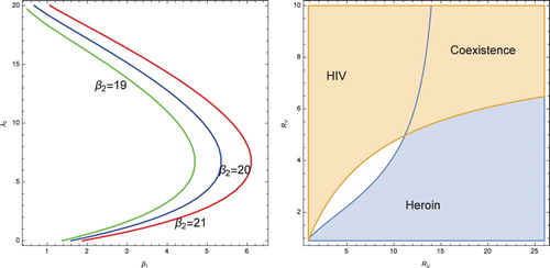
Figure 1 right shows a plot of ${\mathcal{R}}_{vi}^1({\mathcal{R}}_U,{\mathcal{R}}_V)>1$ and ${\mathcal{R}}_{ui}^2({\mathcal{R}}_U,{\mathcal{R}}_V)>1$ in the $({\mathcal{R}}_U,{\mathcal{R}}_V)$ plane. In the blue region, HIV will die out in the population but the heroin epidemic will persist. In the orange region, heroin epidemic will die out in the population but the HIV will persist. In the coexistence region both heroin and HIV will persist. In the white region, where ${\mathcal{R}}_{vi}^1({\mathcal{R}}_U,{\mathcal{R}}_V)<1$ and ${\mathcal{R}}_{ui}^2({\mathcal{R}}_U,{\mathcal{R}}_V)<1$, either heroin epidemic will persist or HIV will persist, dependent on the initial conditions. We surmise that similar tools as in Section 4 will allow us to prove that in the white region there is also a coexistence equilibrium, but that one is very likely unstable, so either semi-trivial equilibrium attracts the solution, depending on the initial conditions.

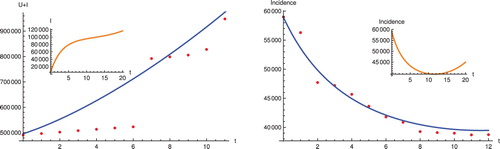
5.2. Understanding the model in relation to US data

To obtain reasonably realistic parameters, we fit the model to heroin use data and HIV cases in the US. We use the heroin use data reported in [23], Figure 2. We transform the percentages in [23] based on the corresponding year US population. We assume children under age of 12 are 50 million, an assumption justified by the data given in [25]. The data on heroin use show an alarming increasing trend. Heroin deaths are also increasing with 60-70% per year [24]. HIV case data in the US can be obtained from a variaty of sources [10,22]. HIV case data in the US are showing steady decline in the past 15 years [22] but recently one can observe stabilization of the number of new cases. We fit the heroin users in a year to $U\left(t\right)+I\left(t\right)$ and the new cases of HIV to the incidence term $I_V\left(t\right)={\lambda }_V\left(t\right)S\left(t\right)+q{\lambda }_V\left(t\right)U\left(t\right)$ using MATLAB to minimize the least square error: $LSE=\sum _{j=0}^n\left(U\right(t_j)-Y_j{)}^2+\sum _{j=0}^m(I_V\left(t_j\right)-y_j{)}^2$ where $Y_j$ and $y_j$ are the y-coordinates of the respective data points and n and m are the number of data points in each data set. The results of the fitting are given in Figure 2. While fitting, we fixed the initial conditions for the ODE system at $S\left(0\right)=45$ million, $U\left(0\right)=491000$, $V\left(0\right)=900000$ and $I\left(0\right)=7000$.

Figure 2. Left: Figure shows fitting of the heroin use data. Right: Figure shows fitting to HIV incidence data. In both figures time is in years where year t = 0 is year 2005. The preestimated and fitted parameters are given in Table 1.

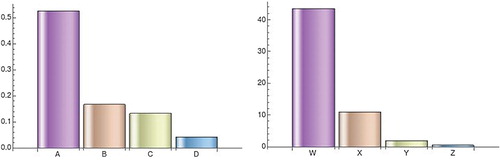
Table 1. Table of fixed and fitted parameter values.

Parameter	Unit	Value	Fixed/fitted
μ	1/year	1/75	fixed
Λ	People/year	400 000 000*μ	fixed
${\text{β}}_1$	1/year	0.3919	fitted
${\text{β}}_2$	1/year	0.06888	fitted
${\mu }_i$	1/year	$0.04783$	fitted
${\mu }_u$	1/year	0.3417	fitted
${\mu }_v$	1/year	0.19	fitted
q	unitless	94.5	fitted
σ	unitless	4.2	fitted
δ	1/year	0.03317	fitted

With the parameters in the table, we estimated ${\mathcal{R}}_U=1.145$ and ${\mathcal{R}}_V=0.362$. Despite the subthreshold value of ${\mathcal{R}}_V$, the invasion numbers are both above one at ${\mathcal{R}}_{vi}^1=8.633$ and ${\mathcal{R}}_{ui}^2=2.174$. Although this scenario is not a part of the analysis, we surmise that the two diseases are in a coexistence regime regardless of the declining incidence of HIV and below one reproduction number. It appears that the heroin epidemic supports the spread of HIV and obstructs it's elimination from the population. It can be observed from the data that the decline in HIV incidence is slowing down, but simulation projections suggest that we can soon expect an increase in incidence if additional control measures are not put into place. Simulations also suggest that the coexistence class is experiencing increase beyond the end of the data.

5.3. Elasticities of the invasion numbers

Elasticities of the invasion numbers are quantities that suggest to which parameters the invasion numbers would be most sensitive. In general, the elasticity of a quantity Q with respect to the parameter p is defined as follows: ${\mathcal{E}}_p^Q=\frac{\mathrm{\partial }Q}{\mathrm{\partial }p}\frac{p}{Q}$ The elasticity ${\mathcal{E}}_p^Q>0$ if Q increases with p and ${\mathcal{E}}_p^Q<0$ if Q decreases with p. The fact that the elasticity of Q with respect to p is ${\mathcal{E}}_p^Q$ means that $1\mathrm{\%}$ increase in p will result in ${\mathcal{E}}_p^Q$ percent change in Q.

We denote the elasticities of the invasion numbers with respect to the reproduction numbers as follows: $A=\frac{\mathrm{\partial }{\mathcal{R}}_{ui}^2}{\mathrm{\partial }{\mathcal{R}}_U}\frac{{\mathcal{R}}_U}{{\mathcal{R}}_{ui}^2}B=\frac{\mathrm{\partial }{\mathcal{R}}_{ui}^2}{\mathrm{\partial }{\mathcal{R}}_V}\frac{{\mathcal{R}}_V}{{\mathcal{R}}_{ui}^2}C=\frac{\mathrm{\partial }{\mathcal{R}}_{vi}^1}{\mathrm{\partial }{\mathcal{R}}_U}\frac{{\mathcal{R}}_U}{{\mathcal{R}}_{vi}^1}D=\frac{\mathrm{\partial }{\mathcal{R}}_{vi}^1}{\mathrm{\partial }{\mathcal{R}}_V}\frac{{\mathcal{R}}_V}{{\mathcal{R}}_{vi}^1}$ Parameters not involved in the reproduction numbers but potentially important for control are q and σ. We denote the elasticities of the invasion numbers with respect to q and σ as follows: $W=\frac{\mathrm{\partial }{\mathcal{R}}_{ui}^2}{\mathrm{\partial }q}\frac{q}{{\mathcal{R}}_{ui}^2}X=\frac{\mathrm{\partial }{\mathcal{R}}_{vi}^1}{\mathrm{\partial }q}\frac{q}{{\mathcal{R}}_{vi}^1}Y=\frac{\mathrm{\partial }{\mathcal{R}}_{ui}^2}{\mathrm{\partial }\sigma }\frac{\sigma }{{\mathcal{R}}_{ui}^2}Z=\frac{\mathrm{\partial }{\mathcal{R}}_{vi}^1}{\mathrm{\partial }\sigma }\frac{\sigma }{{\mathcal{R}}_{vi}^1}$ Figure 3 left and right seems very similar but they are fundamentally different because the y-axis in left goes to 0.5, while the y-axis in right goes to 45. Looking at Figure 3 we see that the invasion numbers are most sensitive to q. Table 1 suggest that heroin users are 94 times more likely to get HIV than non-users. Using heroin increases the HIV risk behaviors, and decreasing the HIV infection in drug users is the most efficient way to decouple the two epidemics. Figure 3 left also suggests that ${\mathcal{R}}_{ui}^2$ is most sensitive to ${\mathcal{R}}_U$. That means that another efficient control measure will be to target hard and strong the heroin epidemic. Interventions that decrease drug use will not only impact positively many lives but also will contribute to decrease in HIV cases.

Figure 3. Left: Figure shows elasticities of the invasion numbers with respect to the reproduction numbers. Right: Figure shows the elasticities of the invasion numbers with respect to q and σ. The parameters used are given in Table 1.

6. Discussion

In this paper, we have studied an HIV/heroin coinfection epidemic model, to describe the co-transmission of heroin and HIV in a single population. The unique disease free equilibrium always exists and it is stable only if both the basic reproduction numbers of heroin and HIV are less than 1, $max\{{\mathcal{R}}_U,{\mathcal{R}}_V\}<1$.

To consider the role of coinfection in our coinfection system, we introduce the invasion reproduction numbers. The invasion reproduction number ${\mathcal{R}}_{ui}^2$ gives the reproduction of the heroin users when the population is at the equilibrium $E_2^{\ast }$, that is, when HIV infection alone is at equilibrium in the single population. The invasion reproduction number ${\mathcal{R}}_{vi}^1$ gives the reproduction of the HIV infection at the equilibrium $E_1^{\ast }$, that is when the heroin transmission alone is at equilibrium in the single population. The local stability of the boundary equilibria $E_1^{\ast }$ and $E_2^{\ast }$ are completely determined by the invasion reproduction numbers. In particular, $E_1^{\ast }$ is locally stable only if ${\mathcal{R}}_{vi}^1<1$ and unstable if ${\mathcal{R}}_{vi}^1>1$. In addition, $E_2^{\ast }$ is locally stable only if ${\mathcal{R}}_{ui}^2<1$ (see Theorems 3.2 – 3.2) and unstable if ${\mathcal{R}}_{ui}^2>1$.

Further, we show that if the two invasion numbers are above one, that is ${\mathcal{R}}_{vi}^1>1$ and ${\mathcal{R}}_{ui}^2>1$, then coexistence equilibrium exists and simulations suggest it is at least locally stable. Further, simulations suggest that parameter regimes exist where two coexistence equilibria are possible. Simulations suggest that the model may have a coexistence equilibrium when ${\mathcal{R}}_{vi}^1<1$ and ${\mathcal{R}}_{ui}^2<1$ but such a coexistence equilibrium is typically unstable. In this case, either heroin use alone will persist in the population or HIV alone will persist in the population, depending on the initial conditions.

Subsection 4.2 also demonstrated the relationship between the invasion reproduction number ${\mathcal{R}}_{ui}^2$ and ${\mathcal{R}}_{vi}^1$. We showed under some assumptions that ${\mathcal{R}}_{ui}^2$ decreases as ${\mathcal{R}}_{vi}^1$ increases and vice versa. This result suggests that the two diseases in many cases are in a competitive mode; however, coinfection leads to the two diseases coexistence, and in part to a ”symbiotic” relationship.

To determine realistic parameters, we compare our model with US data on heroin use and HIV cases. The derive parameters suggest that heroin users are 94 times more likely to get infected by HIV than non-users. These parameters seem to suggest that for the US the two diseases are in strongly coexistence mode with both invasion numbers larger than one. However, we surmise that the coexistence occurs despite the fact that the current reproduction number of HIV in the US is below one. Thus, we think that the heroin epidemic makes possible for the HIV epidemic to continue, regardless of a reproduction number below one. Elasticities of the invasion numbers suggest that control measures must target and tame the heroin epidemic, and success in this direction will likely reduce HIV transmission as well. Further, control measures will be most efficient in decoupling the epidemics, if they are focused on reducing the HIV risk in drug users, that is, they focus on reducing HIV transmission in drug users.

Disclosure statement

No potential conflict of interest was reported by the author(s).

Additional information

Funding

The study was partially supported by the National Natural Science Foundation of China (11771017).

Appendix

(i) To prove that $\mathrm{\partial }{\mathcal{H}}_1/\mathrm{\partial }{\lambda }_1>0$. Note that ${\lambda }_1{g}_1^{\prime }=g_1+{\mu }_i{\lambda }_1^2,{\lambda }_2{g}_2^{\prime }{\lambda }_1={\lambda }_2{g}_2+{\lambda }_{2}q{\lambda }_1^2.$ By use of the expressions of $A_{11}$ and $A_{12}$, we have $\begin{array}{rl}\frac{\mathrm{\partial }{A}_{11}}{\mathrm{\partial }{\lambda }_1}{A}_{12}-A_{11}\frac{\mathrm{\partial }{A}_{12}}{\mathrm{\partial }{\lambda }_1}& =\left(g_1^{\prime }\right({\lambda }_1)+{\lambda }_2{g}_2^{\prime }({\lambda }_1)+g_3({\lambda }_2\left)\right)\left(g_4\right({\lambda }_2\left)g_5\right({\lambda }_1)+g_6({\lambda }_2)+\sigma \delta q{\lambda }_1{\lambda }_2)\\ & -\left(g_1\right({\lambda }_1)+{\lambda }_2{g}_2({\lambda }_1)+{\lambda }_1{g}_3({\lambda }_2\left)\right)\left(g_4\right({\lambda }_2\left)g_5^{\prime }\right({\lambda }_1)+\sigma \delta q{\lambda }_2)\\ & =\left(g_1^{\prime }\right({\lambda }_1)+{\lambda }_2{g}_2^{\prime }({\lambda }_1)+g_3({\lambda }_2\left)\right)\sigma \delta q{\lambda }_1{\lambda }_2\\ & -\left(g_1\right({\lambda }_1)+{\lambda }_2{g}_2({\lambda }_1)+{\lambda }_1{g}_3({\lambda }_2\left)\right)\sigma \delta q{\lambda }_2\\ & +\left(g_1^{\prime }\right({\lambda }_1)+{\lambda }_2{g}_2^{\prime }({\lambda }_1)+g_3({\lambda }_2\left)\right)\left(g_4\right({\lambda }_2\left)g_5\right({\lambda }_1)+g_6({\lambda }_2\left)\right)\\ & -\left(g_1\right({\lambda }_1)+{\lambda }_2{g}_2({\lambda }_1)+{\lambda }_1{g}_3({\lambda }_2\left)\right)g_4\left({\lambda }_2\right)g_5^{\prime }\left({\lambda }_1\right)\\ & =({\mu }_i{\lambda }_1^2+{\lambda }_{2}q{\lambda }_1^2)\sigma \delta q{\lambda }_2\\ & +\frac{1}{{\lambda }_1}[{\lambda }_1\left(g_1^{\prime }\right({\lambda }_1)+{\lambda }_2{g}_2^{\prime }({\lambda }_1)+g_3({\lambda }_2\left)\right)\left(g_4\right({\lambda }_2\left)g_5\right({\lambda }_1)+g_6({\lambda }_2\left)\right)\\ & -\left(g_1\right({\lambda }_1)+{\lambda }_2{g}_2({\lambda }_1)+{\lambda }_1{g}_3({\lambda }_2\left)\right)g_4\left({\lambda }_2\right){\mu }_i{\lambda }_1]\\ & =({\mu }_i{\lambda }_1^2+{\lambda }_{2}q{\lambda }_1^2)\sigma \delta q{\lambda }_2+\left(g_1^{\prime }\right({\lambda }_1)+{\lambda }_2{g}_2^{\prime }({\lambda }_1)+g_3({\lambda }_2\left)\right)g_6\left({\lambda }_2\right)+B_{12},\end{array}$ where $\begin{array}{rl}{B}_{12}& =\frac{1}{{\lambda }_1}[{\lambda }_1\left(g_1^{\prime }\right({\lambda }_1)+{\lambda }_2{g}_2^{\prime }({\lambda }_1)+g_3({\lambda }_2\left)\right)g_4\left({\lambda }_2\right)g_5\left({\lambda }_1\right)\\ & -\left(g_1\right({\lambda }_1)+{\lambda }_2{g}_2({\lambda }_1)+{\lambda }_1{g}_3({\lambda }_2\left)\right)g_4\left({\lambda }_2\right){\mu }_i{\lambda }_1]\\ & =\frac{1}{{\lambda }_1}[(g_1+{\mu }_i{\lambda }_1^2+q{\lambda }_1^2{\lambda }_2+{\lambda }_2{g}_2+{\lambda }_1{g}_3)({\mu }_i{\lambda }_1+(\sigma \delta +{\mu }_i\left){\mu }_v\right)g_4\\ & -(g_1+{\lambda }_2{g}_2+{\lambda }_1{g}_3){\mu }_i{\lambda }_1{g}_4]\\ & =\frac{1}{{\lambda }_1}[(g_1+{\mu }_i{\lambda }_1^2+q{\lambda }_1^2{\lambda }_2+{\lambda }_2{g}_2+{\lambda }_1{g}_3)(\sigma \delta +{\mu }_i){\mu }_v{g}_4+({\mu }_i{\lambda }_1^2+q{\lambda }_1^2{\lambda }_2){\mu }_i{\lambda }_1{g}_4]>0.\end{array}$ Note that $g_1^{\prime }>0$, $g_2^{\prime }>0$. Then we have $\frac{\mathrm{\partial }{A}_{11}}{\mathrm{\partial }{\lambda }_1}{A}_{12}-A_{11}\frac{\mathrm{\partial }{A}_{12}}{\mathrm{\partial }{\lambda }_1}>0\Rightarrow \frac{\mathrm{\partial }{\mathcal{H}}_1}{\mathrm{\partial }{\lambda }_1}>0.$ (ii) By use of the expressions of $A_{11}$ and $A_{12}$, we have $\begin{array}{rl}\frac{\mathrm{\partial }{A}_{11}}{\mathrm{\partial }{\lambda }_2}{A}_{12}-A_{11}\frac{\mathrm{\partial }{A}_{12}}{\mathrm{\partial }{\lambda }_2}& =(g_2+{\lambda }_1{g}_3^{\prime })(g_4{g}_5+g_6+\sigma \delta q{\lambda }_1{\lambda }_2)\\ & -(g_1+{\lambda }_2{g}_2+{\lambda }_1{g}_3)(g_4^{\prime }{g}_5+g_6^{\prime }+\sigma \delta q{\lambda }_1)\\ & =(g_2+{\lambda }_1{g}_3^{\prime })(g_4{g}_5+g_6)-(g_1+{\lambda }_2{g}_2+{\lambda }_1{g}_3)(g_4^{\prime }{g}_5+g_6^{\prime })\\ & +(g_2+{\lambda }_1{g}_3^{\prime })\sigma \delta q{\lambda }_1{\lambda }_2-(g_1+{\lambda }_2{g}_2+{\lambda }_1{g}_3)\sigma \delta q{\lambda }_1\\ & =\frac{1}{{\lambda }_2}[{\lambda }_2(g_2+{\lambda }_1{g}_3^{\prime })(g_4{g}_5+g_6)-(g_1+{\lambda }_2{g}_2+{\lambda }_1{g}_3)(g_4^{\prime }{g}_5+g_6^{\prime }){\lambda }_2]\\ & +({\lambda }_2{g}_2+{\lambda }_1{g}_3+{\lambda }_{1}q{\lambda }_2^2)\sigma \delta q{\lambda }_1-(g_1+{\lambda }_2{g}_2+{\lambda }_1{g}_3)\sigma \delta q{\lambda }_1\\ & =\frac{1}{{\lambda }_2}[({\lambda }_2{g}_2+{\lambda }_1{g}_3+{\lambda }_{1}q{\lambda }_2^2)(g_4{g}_5+g_6)\\ & -({\lambda }_2{g}_2+{\lambda }_1{g}_3)(q{g}_5{\lambda }_2+g_6+q{\lambda }_2^2(\sigma \delta +{\mu }_i\left)\right)]\\ & +q^2{\lambda }_1^2{\lambda }_2^2\sigma \delta -g_1\sigma \delta q{\lambda }_1-g_1(q{g}_5+g_6^{\prime })\\ & =\frac{1}{{\lambda }_2}[{\lambda }_{1}q{\lambda }_2^2{g}_4{g}_5+{\lambda }_{1}q{\lambda }_2^2{g}_6+({\lambda }_2{g}_2+{\lambda }_1{g}_3){\mu }_u{g}_5\\ & -{\lambda }_2{g}_{2}q{\lambda }_2^2(\sigma \delta +{\mu }_i)-{\lambda }_1{g}_{3}q{\lambda }_2^2(\sigma \delta +{\mu }_i)]\\ & +q^2{\lambda }_1^2{\lambda }_2^2\sigma \delta -g_1\sigma \delta q{\lambda }_1-g_1(q{g}_5+g_6^{\prime })\\ & =q{g}_3{g}_1+{\mu }_u{g}_2{g}_5+\frac{1}{{\lambda }_2}{\mu }_u{g}_3{g}_1-g_{2}q{\lambda }_2^2(\sigma \delta +{\mu }_i)\\ & +q^2{\lambda }_1^2{\lambda }_2^2\sigma \delta -g_1\sigma \delta q{\lambda }_1-g_1(q{g}_5+g_6^{\prime })\\ & =q{g}_3{g}_1+{\mu }_u{g}_2{g}_5+\frac{1}{{\lambda }_2}{\mu }_u{g}_3{g}_1-g_1\sigma \delta q{\lambda }_1\\ & -g_1\left(q{g}_5+(\sigma \delta +{\mu }_i)\frac{1}{{\lambda }_2}{g}_3+q{\lambda }_2(\sigma \delta +{\mu }_i)\right)\\ & -q^2{\lambda }_1{\lambda }_2^2({\lambda }_1+{\mu }_v)(\sigma \delta +{\mu }_i)+q^2{\lambda }_1^2{\lambda }_2^2\sigma \delta \\ & =q{g}_3{g}_1+{\mu }_u{g}_2{g}_5-g_1\sigma \delta q{\lambda }_1-g_{1}q{g}_5-g_{1}q{\lambda }_2(\sigma \delta +{\mu }_i)\\ & -\frac{1}{{\lambda }_2}{g}_3{g}_1(\sigma \delta +{\mu }_i-{\mu }_u)-q^2{\lambda }_2^2{g}_1\\ & =B_{21}+B_{22},\end{array}$ where $\begin{array}{rl}{B}_{21}& ={\mu }_u{g}_2{g}_5-g_1\sigma \delta q{\lambda }_1-g_{1}q{g}_5\\ & =g_5[{\mu }_u{\lambda }_{1}q({\lambda }_1+{\mu }_v)-\sigma \delta q{\lambda }_1^2-q{\lambda }_1({\mu }_i{\lambda }_1+(\sigma \delta +{\mu }_i\left){\mu }_v\right)]\\ & =g_5[{\mu }_{u}q{\lambda }_1^2-\sigma \delta q{\lambda }_1^2-q{\lambda }_1^2{\mu }_i-q{\lambda }_1(\sigma \delta +{\mu }_i){\mu }_v+{\mu }_{u}q{\lambda }_1{\mu }_v]\\ & =-g_5(\sigma \delta +{\mu }_i-{\mu }_u)[q{\lambda }_1^2+q{\lambda }_1{\mu }_v]<0,\\ B_{22}& =q{g}_3{g}_1-g_{1}q{\lambda }_2(\sigma \delta +{\mu }_i)-\frac{1}{{\lambda }_2}{g}_3{g}_1(\sigma \delta +{\mu }_i-{\mu }_u)-q^2{\lambda }_2^2{g}_1\\ & =g_{1}q{\lambda }_2(q{\lambda }_2+{\mu }_u)-g_{1}q{\lambda }_2(\sigma \delta +{\mu }_i)-(q{\lambda }_2+{\mu }_u)g_1(\sigma \delta +{\mu }_i-{\mu }_u)-q^2{\lambda }_2^2{g}_1\\ & =-g_{1}q{\lambda }_2(\sigma \delta +{\mu }_i-{\mu }_u)-(q{\lambda }_2+{\mu }_u)g_1(\sigma \delta +{\mu }_i-{\mu }_u)\\ & =-(2q{\lambda }_2+{\mu }_u)g_1(\sigma \delta +{\mu }_i-{\mu }_u)<0.\end{array}$ In the above proofs, we have used that $\sigma \ge 1$ and $d_I\ge d_U$, i.e. $(\sigma \delta +{\mu }_i-{\mu }_u)>0$. Thus, we obtain $\frac{\mathrm{\partial }{A}_{11}}{\mathrm{\partial }{\lambda }_2}{A}_{12}-A_{11}\frac{\mathrm{\partial }{A}_{12}}{\mathrm{\partial }{\lambda }_2}<0,$ and therefore $\mathrm{\partial }{\mathcal{H}}_1({\lambda }_1,{\lambda }_2)/\mathrm{\partial }{\lambda }_2<0$.

References

- S. Alizon, Co-infection and super-infection models in evolutionary epidemiology, Interface Focus 3(6) (2013), pp. 20130031. doi: 10.1098/rsfs.2013.0031
- L.J. Abu-Raddad, P. Patnaik, and J.G. Kublin, Dual infection with HIV and malaria fuels the spread of both diseases in sub-Saharan Africa, Science 314(5805) (2006), pp. 1603–1606. doi: 10.1126/science.1132338
- K.B. Blyuss and Y.N. Kyrychko, On a basic model of a two-disease epidemic, Appl. Math. Comput. 160(1) (2005), pp. 177–187.
- O. Diekmann, J.A.P. Heesterbeek, and J.A.J. Metz, On the definition and the computation of the basic reproduction ratio R0 in models for infectious diseases in heterogeneous populations, J. Math. Biol. 28(4) (1990), pp. 365–382. doi: 10.1007/BF00178324
- P. van den Driessche and J. Watmough, Reproduction numbers and sub-threshold endemic equilibria for compartmental models of disease transmission, Math. Biosci. 180 (2002), pp. 29–48. doi: 10.1016/S0025-5564(02)00108-6
- D.R. Mackintosh and G.T. Stewart, A mathematical model of a heroin epidemic: implications for control policies, J. Epidemiol. Community Health 33(4) (1979), pp. 299–304. doi: 10.1136/jech.33.4.299
- European Monitoring Centre for Drugs and Drug Addiction (EMCDDA): Annual Report, 2005. http://annualreport.emcdda.eu.int/en/homeen.html.
- B. Fang, X-Z. Li, M. Martcheva, and L-M. Cai, Global asymptotic properties of a heroin epidemic model with treat-age, Appl. Math. Comput. 263 (2015), pp. 315–331.
- D. Gao, T.C. Porco, and S. Ruan, Coinfection dynamics of two diseases in a single host population, J. Math. Anal. Appl. 442 (2016), pp. 171–188. doi: 10.1016/j.jmaa.2016.04.039
- H.I. Hall, R. Song, P. Rhodes, J. Prejean, Q. An, L.M. Lee, J. Karon, R. Brookmeyer, E.H. Kaplan, M.T. McKenna, and R.S. Janssen, HIV incidence surveillance group. Estimation of HIV incidence in the United States, JAMA 300(5) (Aug 6 2008), pp. 520–529. doi:10.1001/jama.300.5.520
- M. Iannelli, M. Martcheva, and X.Z. Li, Strain replacement in an epidemic model with super-infection and perfect vaccination, Math. Biosci. 195(1) (2005), pp. 23–46. doi: 10.1016/j.mbs.2005.01.004
- M.J. Keeling and P. Rohani, Modeling Infectious Diseases in Humans and Animals, Princeton University Press, Princeton, 2008.
- A. Kelly, M. Carvalho, and C. Teljeur, Prevalence of Opiate Use in Ireland 2000-2001. A 3-Source Capture Recapture Study. A Report to the National Advisory Committee on Drugs, Subcommittee on Prevalence. Small Area Health Research Unit, Department of Public
- G. Lawi, J. Mugisha, and N. Omolo-Ongati, Mathematical model for malaria and meningitis co-infection among children, Appl. Math. Sci. 5(47) (2011), pp. 2337–2359.
- X-Z. Li, X. Duan, M. Ghosh, and X-Y Ruan, Pathogen coexistence induced by saturating contact rates, Nonlinear Anal-Real. 10 (2009), pp. 3298–3311. doi: 10.1016/j.nonrwa.2008.10.038
- M. Martcheva and S.S. Pilyugin, The role of coinfection in multidisease dynamics, SIAM J. Appl. Math. 66 (2006), pp. 843–872. doi: 10.1137/040619272
- M. Martcheva, S.S. Pilyugin, and R.D. Holt, Subthreshold and superthreshold coexistence of pathogen variants: the impact of host age-structure, Math. Biosci. 207(1) (2007), pp. 58–77. doi: 10.1016/j.mbs.2006.09.010
- S. Mushayabasa, J. Tchuenche, C. Bhunu, and E. Ngarakana-Gwasira, Modeling gonorrhea and HIV co-interaction, BioSystems 103(1) (2011), pp. 27–37. doi: 10.1016/j.biosystems.2010.09.008
- L. Roeger, Z. Feng, and C. Castillo-Chavez, Modeling TB and HIV co-infections, Math. Biosci. Eng.6(4) (2009), pp. 815–837. doi: 10.3934/mbe.2009.6.815
- T. Porco and S. Blower, HIV vaccines: the effect of the mode of action on the coexistence of HIV subtypes, Math. Popul. Studies. 8 (2000), pp. 205–229. doi: 10.1080/08898480009525481
- O. Sharomi, C.N. Podder, A.B. Gumel, and B. Song, Mathematical analysis of the transmission dynamics of HIV/TB control in the presence of treatment, Math. Biosci. Eng. 5 (2008), pp. 145–174. doi: 10.3934/mbe.2008.5.145
- https://www.cdc.gov/hiv/pdf/policies/cdc-hiv-2015-dhap-annual-report.pdf
- https://www.samhsa.gov/data/sites/default/files/NSDUH-FFR1-2016/NSDUH-FFR1-2016.pdf
- https://catalog.data.gov/dataset/total-number-of-drug-intoxication-deaths-by-selected-substances-2007-2016
- https://datacenter.kidscount.org/data/tables/101-child-population-by-age-group#detailed/1/any/false/871,870,573,869,36,868,867,133,38,35/62,63,64,6,4693/419,420
Appendix
(i) To prove that . Note that
By use of the expressions of
and
, we have
where
Note that
,
. Then we have
(ii) By use of the expressions of
In the above proofs, we have used that
, i.e.
. Thus, we obtain
and therefore