Balance simplices of 3-species May-Leonard systems

Abstract

We investigate the existence of a two-dimensional invariant manifold that attracts all nonzero orbits in 3 species Lotka-Volterra systems with identical linear growth rates. This manifold, which we call the balance simplex, is the common boundary of the basin of repulsion of the origin and the basin of repulsion of infinity. The balance simplex is linked to ecological models where there is ‘growth when rare’ and competition for finite resources. By including alternative food sources for predators we cater for predator-prey type models. In the case that the model is competitive, the balance simplex coincides with the carrying simplex which is an unordered manifold (no two points may be ordered componentwise), but for non-competitive models the balance simplex need not be unordered. The balance simplex of our models contains all limit sets and is the graph of a piecewise analytic function over the unit probability simplex.

Keywords:

• Balance simplex
• Lotka-Volterra
• invariant manifold
• stability basin boundaries

2010 Mathematics Subject Classifications:

• 24C45
• 37D10
• 92D40

1. Introduction

Recently in [8] we studied the dynamics of the planar system (1) ${\dot{x}}_1=x_1(1-x_1-\alpha x_2),{\dot{x}}_2=x_2(1-x_2-\text{β}{x}_1)$(1) on the first quadrant, where $\alpha ,\text{β}\in \mathbb{R}$, not necessarily positive. Equation (1(1) ${\dot{x}}_1=x_1(1-x_1-\alpha x_2),{\dot{x}}_2=x_2(1-x_2-\text{β}{x}_1)$(1) ) differs from the most general planar Lotka-Volterra model since the two species linear growth rates are the same and scaled to unity. We showed that when $\alpha ,\text{β}$ are chosen such that orbits of (1(1) ${\dot{x}}_1=x_1(1-x_1-\alpha x_2),{\dot{x}}_2=x_2(1-x_2-\text{β}{x}_1)$(1) ) are bounded, there exists an invariant manifold Σ which attracts all points in the first quadrant minus the origin and that projects radially one-to-one and onto the unit probability simplex ${\mathrm{\Delta }}_2=\left\{\right(u,1-u):0\le u\le 1\}$. We named Σ the balance simplex, as it is the analogue of the carrying simplex found in competitive systems, and consists of points on the common boundary of the basin of repulsion of the origin and infinity, but unlike the carrying simplex it is not typically an unordered manifold (a manifold is unordered if no two points have coordinates that can be ordered componentwise). The relative simplicity of (1(1) ${\dot{x}}_1=x_1(1-x_1-\alpha x_2),{\dot{x}}_2=x_2(1-x_2-\text{β}{x}_1)$(1) ) meant that we were able to give explicit expressions for the balance manifold in terms of Gauss hypergeometric functions.

In a second paper [7] we put forward biologically reasonable conditions for the existence of a balance simplex in planar Kolmogorov systems with at most one interior equilibrium which is then hyperbolic. The conditions include that the origin and infinity are repellers, there exists exactly one non-zero and hyperbolic equilibrium on each axis and all nonzero orbits on an axis are attracted to this axial equilibrium, and that there is intraspecific competition which prevents interior periodic orbits. We also presented a series of examples of systems with a variety of competitive, cooperative and predator-prey interactions to illustrate our results.

The ecological importance of these findings is that under biologically reasonable conditions, at least in the case where there is at most one coexistence equilibrium, there is a curve on which the effects of growth when rare, and  competition for finite resources balance; hence the choice of the name ‘balance’ simplex. No community with all species present can completely collapse – at least one species must remain extant (and finite).

Here we show that a suitably defined and piecewise analytic balance simplex also exists for the following natural 3-species extension of (1(1) ${\dot{x}}_1=x_1(1-x_1-\alpha x_2),{\dot{x}}_2=x_2(1-x_2-\text{β}{x}_1)$(1) ), known as the May-Leonard system [17]: (2) ${\dot{x}}_i=F_i\left(x\right)=x_i{f}_i\left(x\right)=x_i(1-(Ax{)}_i),i=1,2,3$(2) where $x=(x_1,x_2,x_3)$, A is a real $3\times 3$ matrix with elements $a_{ij}$ for i, j = 1, 2, 3 and $a_{ii}=1$ for i = 1, 2, 3. This model was studied by May and Leonard in the context of its heteroclinic cycles. Since (2(2) ${\dot{x}}_i=F_i\left(x\right)=x_i{f}_i\left(x\right)=x_i(1-(Ax{)}_i),i=1,2,3$(2) ) is a model for population dynamics, we restrict to the invariant positive cone $K={\mathbb{R}}_{+}^3$, where ${\mathbb{R}}_{+}:=[0,\mathrm{\infty })$. We emphasize that we do not assume that A has non-negative elements, so that we are not confining our analysis to competitive systems.

Here the balance simplex is defined via:

Definition 1.1

A balance simplex Σ of a semiflow on K is a subset of K with the following properties:

1. Σ is invariant, compact, and projects radially 1-1 and onto the unit probability simplex;

2. Σ globally attracts all non-zero points in K and is asymptotically complete (i.e. given $x\in K\setminus \left\{0\right\}$ there exists a $y\in \mathrm{\Sigma }$ such that $\parallel x\left(t\right)-y\left(t\right)\parallel \to 0$ as $t\to \mathrm{\infty }$).

($x\left(t\right)$ is the forward evolution of x under the semiflow, and similarly for y).

Definition 1.1 slightly differs from Definition 2.1 in [8] as it includes asymptotic completeness of the manifold. This is a natural requirement since it ensures that the full flow of (2(2) ${\dot{x}}_i=F_i\left(x\right)=x_i{f}_i\left(x\right)=x_i(1-(Ax{)}_i),i=1,2,3$(2) ) can be approximated by a flow on Σ, and this approximation is most useful when orbits approach Σ rapidly, such as when Σ is also an inertial manifold.

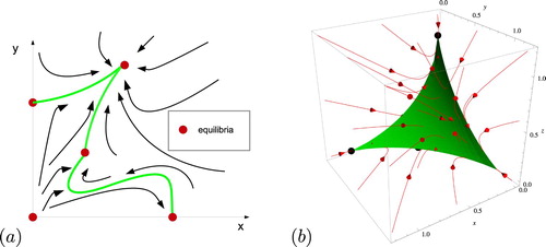
When Σ is also unordered, so that no two distinct points x, y of Σ satisfy $x-y\in K$, such as when (1(1) ${\dot{x}}_1=x_1(1-x_1-\alpha x_2),{\dot{x}}_2=x_2(1-x_2-\text{β}{x}_1)$(1) ) is competitive, the balance simplex coincides with the carrying simplex of Hirsch [11, 12]. In Figure 1(a) we illustrate the idea of the balance simplex as the common boundary of the basin of repulsion and infinity that projects radially one-to-one onto the unit probability simplex. Figure 1(b) shows a carrying simplex and a sample of orbits for the competitive May-Leonard system (2(2) ${\dot{x}}_i=F_i\left(x\right)=x_i{f}_i\left(x\right)=x_i(1-(Ax{)}_i),i=1,2,3$(2) ).

Figure 1. (a) The balance simplex. (b) A representative example of the carrying simplex and a sample of orbits for a competitive case (i.e. $a_{ij}\ge 0$ for $i\ne j$) of the May-Leonard system (2(2) ${\dot{x}}_i=F_i\left(x\right)=x_i{f}_i\left(x\right)=x_i(1-(Ax{)}_i),i=1,2,3$(2) ). In both (a) and (b) the green manifold is the balance simplex and it attracts all nonzero orbits.

The May-Leonard system was introduced in [17] and has been studied under various constraints on the matrix A to include competition, cooperation and predator-prey interactions (e.g. [6, 22]).

2. The result

We recall that a $3\times 3$ real matrix A is copositive when $x\cdot Ax\ge 0$ for $x\in K$ and strictly copositive when $x\cdot Ax>0$ for $x\in K\setminus \left\{0\right\}$. Note that $2x\cdot Ax=x\cdot (A+A^T)x$ so we need only check whether the symmetric matrix $(A+A^T)$ is copositive or strictly copositive.

Lemma 2.1

The real symmetric matrix $B=\left(\begin{array}{ccc}1& \alpha & \text{β}\\ \alpha & 1& \gamma \\ \text{β}& \gamma & 1\end{array}\right)$ is strictly copositive if and only if $\alpha ,\text{β},\gamma$ satisfy $min\{\alpha ,\text{β},\gamma \}>-1$ and at least one of the following two conditions hold: (3) $\begin{array}{rl}& \alpha +\text{β}+\gamma +1>0\end{array}$(3) (4) $\begin{array}{rl}& 1+2\alpha \text{β}\gamma -{\alpha }^2-{\text{β}}^2-{\gamma }^2>0.\end{array}$(4)

Proof.

This follows easily from [10].

We recall that the Replicator system on the 2-dimensional unit probability simplex $\mathrm{\Delta }=\{u\in K:\sum _{i=1}^3{u}_i=1\}$ for matrix games with 3 strategies is the system of differential equations [21] (5) ${\dot{u}}_i=u_i\left(\right(Au{)}_i-u\cdot Au),i=1,2,3,u(0)\in \mathrm{\Delta }.$(5) For a background on this system see, for example, [13].

We recall that given a flow, the basin of attraction of an equilibrium p is the set of points that converge to p under the flow forwards in time, and the basin of repulsion of an equilibrium p is the set of points that converge to p under the flow backwards in time.

Here we will prove:

Theorem 2.2

If the $3\times 3$ matrix A is strictly copositive, then the system (2(2) ${\dot{x}}_i=F_i\left(x\right)=x_i{f}_i\left(x\right)=x_i(1-(Ax{)}_i),i=1,2,3$(2) ) has a balance simplex and there is a continuous function $\mathrm{\Psi }:\mathrm{\Delta }\to {\mathbb{R}}_{+}$ such that $\mathrm{\Sigma }=\left\{\mathrm{\Psi }\right(u)u:u\in \mathrm{\Delta }\}\subset K$ and Σ is the common boundary relative to K of the basins of repulsion of the origin and infinity.

If in addition (i) all equilibria of the planar Replicator system (5(5) ${\dot{u}}_i=u_i\left(\right(Au{)}_i-u\cdot Au),i=1,2,3,u(0)\in \mathrm{\Delta }.$(5) ) with fitness matrix A are isolated and hyperbolic, and (ii) every trajectory of (5(5) ${\dot{u}}_i=u_i\left(\right(Au{)}_i-u\cdot Au),i=1,2,3,u(0)\in \mathrm{\Delta }.$(5) ) converges to an equilibrium, then Ψ is piecewise analytic on Δ, with discontinuous gradients only possible at equilibria or across heteroclinic orbits that lie in the interior of Δ.

3. Existence of the balance simplex

As a first step we introduce new coordinates R and $u=(u_1,u_2,u_3)\in \mathrm{△}$ with $R=\sum _{i=1}^3{x}_i$ and $u_i=x_i/R$ for i = 1, 2, 3. Thus we work with total population density R and species frequencies u. We will assume that A is strictly copositive so that the mean fitness $u\cdot Au>0$ for $u\in \mathrm{\Delta }$.

In the new coodinates (2(2) ${\dot{x}}_i=F_i\left(x\right)=x_i{f}_i\left(x\right)=x_i(1-(Ax{)}_i),i=1,2,3$(2) ) transforms into the equivalent system (6) $\begin{array}{rl}\dot{R}& =R(1-u\cdot AuR)\end{array}$(6) (7) $\begin{array}{rl}{\dot{u}}_i& =R{u}_i(u\cdot Au-(Au{)}_i),i=1,2,3.\end{array}$(7) We note that (6(6) $\begin{array}{rl}\dot{R}& =R(1-u\cdot AuR)\end{array}$(6) ) is logistic growth of the total population with unit linear growth rate and time-dependent carrying capacity $(u\cdot Au{)}^{-1}$ (which is defined since A is strictly copositive). On the other hand (7(7) $\begin{array}{rl}{\dot{u}}_i& =R{u}_i(u\cdot Au-(Au{)}_i),i=1,2,3.\end{array}$(7) ) is the standard replicator system for matrix games, but with time rescaled and run backwards. We will exploit this partial decoupling of the dynamics in what follows by scaling time.

The reduction of (2(2) ${\dot{x}}_i=F_i\left(x\right)=x_i{f}_i\left(x\right)=x_i(1-(Ax{)}_i),i=1,2,3$(2) ) to (6(6) $\begin{array}{rl}\dot{R}& =R(1-u\cdot AuR)\end{array}$(6) ), (7(7) $\begin{array}{rl}{\dot{u}}_i& =R{u}_i(u\cdot Au-(Au{)}_i),i=1,2,3.\end{array}$(7) ), which relies on identical linear growth rates is crucial, has been previously exploited by a number of authors [5, 24].

If A is strictly copositive, by compactness of $\mathrm{△}$ there is a $\delta >0$ such that $u\cdot Au\ge \delta >0$ for all $u\in \mathrm{△}$. From (6(6) $\begin{array}{rl}\dot{R}& =R(1-u\cdot AuR)\end{array}$(6) ) we see that $\dot{R}<R(1-\delta R)$ which tells us that the total population R eventually falls below $\frac{1}{\delta }$. Thus the assumption that A is strictly copositive implies that all orbits of (6(6) $\begin{array}{rl}\dot{R}& =R(1-u\cdot AuR)\end{array}$(6) ), (7(7) $\begin{array}{rl}{\dot{u}}_i& =R{u}_i(u\cdot Au-(Au{)}_i),i=1,2,3.\end{array}$(7) ) and equivalently the original system (2(2) ${\dot{x}}_i=F_i\left(x\right)=x_i{f}_i\left(x\right)=x_i(1-(Ax{)}_i),i=1,2,3$(2) ) remain bounded for all forward time.

Since $-u\cdot Au=\frac{\mathrm{\partial }}{\mathrm{\partial }R}\left(\frac{\dot{R}}{R}\right)$ we may interpret copositivity of A as meaning that the per-capita growth rate averaged over the whole population decreases as the total population size increases, regardless of the frequency of each species (even if some, but not all, are extinct).

For a given initial point $(u_0,R_0)\in \mathrm{\Delta }\times {\mathbb{R}}_{+}$ we denote the unique trajectory of (6(6) $\begin{array}{rl}\dot{R}& =R(1-u\cdot AuR)\end{array}$(6) ), (7(7) $\begin{array}{rl}{\dot{u}}_i& =R{u}_i(u\cdot Au-(Au{)}_i),i=1,2,3.\end{array}$(7) ) by $t\mapsto \left(u\right(u_0,R_0,t),R(u_0,R_0,t\left)\right),t\in {\mathbb{R}}_{+}$.

The origin $\mathcal{O}$ is a repeller of (2(2) ${\dot{x}}_i=F_i\left(x\right)=x_i{f}_i\left(x\right)=x_i(1-(Ax{)}_i),i=1,2,3$(2) ) and its basin of repulsion is the open set $\mathcal{R}\left(\mathcal{O}\right)=\left\{R_0{u}_0:u_0\in \mathrm{\Delta },R_0\ge 0,\underset{t\to -\mathrm{\infty }}{lim}R(u_0,R_0,t)=0\right\}.$ We are interested in the boundary of $\mathcal{R}\left(\mathcal{O}\right)$ relative to K, which we denote by $\mathrm{\partial }\mathcal{R}\left(\mathcal{O}\right)$. Indeed we will show that, under the assumptions of Theorem 2.2, (2(2) ${\dot{x}}_i=F_i\left(x\right)=x_i{f}_i\left(x\right)=x_i(1-(Ax{)}_i),i=1,2,3$(2) ) has $\mathrm{\partial }\mathcal{R}\left(\mathcal{O}\right)$ as a balance simplex Σ with $\mathrm{\Sigma }=\mathrm{\partial }\mathcal{R}\left(\mathrm{\infty }\right)=\mathrm{\partial }\mathcal{R}\left(\mathcal{O}\right)$.

For convenience, we will now run time backwards and study, in place of (6(6) $\begin{array}{rl}\dot{R}& =R(1-u\cdot AuR)\end{array}$(6) ), (7(7) $\begin{array}{rl}{\dot{u}}_i& =R{u}_i(u\cdot Au-(Au{)}_i),i=1,2,3.\end{array}$(7) ), the system (8) $\begin{array}{rl}& \frac{\mathrm{d}S}{\mathrm{d}s}=S(u\cdot AuS-1)\end{array}$(8) (9) $\begin{array}{rl}& \frac{\mathrm{d}{u}_i}{\mathrm{d}s}=S{u}_i\left(\right(Au{)}_i-u\cdot Au),i=1,2,3.\end{array}$(9) The orbits of the systems (6(6) $\begin{array}{rl}\dot{R}& =R(1-u\cdot AuR)\end{array}$(6) ),(7(7) $\begin{array}{rl}{\dot{u}}_i& =R{u}_i(u\cdot Au-(Au{)}_i),i=1,2,3.\end{array}$(7) ) and (8(8) $\begin{array}{rl}& \frac{\mathrm{d}S}{\mathrm{d}s}=S(u\cdot AuS-1)\end{array}$(8) ),(9(9) $\begin{array}{rl}& \frac{\mathrm{d}{u}_i}{\mathrm{d}s}=S{u}_i\left(\right(Au{)}_i-u\cdot Au),i=1,2,3.\end{array}$(9) ) are identical, but for the dynamics generated by (8(8) $\begin{array}{rl}& \frac{\mathrm{d}S}{\mathrm{d}s}=S(u\cdot AuS-1)\end{array}$(8) ), (9(9) $\begin{array}{rl}& \frac{\mathrm{d}{u}_i}{\mathrm{d}s}=S{u}_i\left(\right(Au{)}_i-u\cdot Au),i=1,2,3.\end{array}$(9) ), $\mathcal{O}$ is now an attractor, and we are now interested in the finding the basin of attraction of $\mathcal{O}$: $\mathcal{B}\left(\mathcal{O}\right)=\left\{S_0{u}_0:u_0\in \mathrm{\Delta },S_0\ge 0,\underset{s\to \mathrm{\infty }}{lim}S(u_0,S_0,s)=0\right\}.$ The boundary of $\mathcal{B}\left(\mathcal{O}\right)$ relative to K is denoted by $\mathrm{\partial }\mathcal{B}\left(\mathcal{O}\right)$.

Fix a $u_0\in \mathrm{\Delta }$ and $S_0>0$ and let $s\mapsto \left(u\right(u_0,S_0,s),S(u_0,S_0,s\left)\right)$ denote the unique trajectory of (8(8) $\begin{array}{rl}& \frac{\mathrm{d}S}{\mathrm{d}s}=S(u\cdot AuS-1)\end{array}$(8) ), (9(9) $\begin{array}{rl}& \frac{\mathrm{d}{u}_i}{\mathrm{d}s}=S{u}_i\left(\right(Au{)}_i-u\cdot Au),i=1,2,3.\end{array}$(9) ) through $(u_0,S_0)$ defined for $s\in [0,s_{max}(u_0,S_0\left)\right)$, where $s_{max}(u_0,S_0)$ is the maximal range of s for which the orbit of (8(8) $\begin{array}{rl}& \frac{\mathrm{d}S}{\mathrm{d}s}=S(u\cdot AuS-1)\end{array}$(8) ), (9(9) $\begin{array}{rl}& \frac{\mathrm{d}{u}_i}{\mathrm{d}s}=S{u}_i\left(\right(Au{)}_i-u\cdot Au),i=1,2,3.\end{array}$(9) ) through $(u_0,S_0)$ is bounded. $s_{max}(u_0,S_0)$ may be finite, as it is possible for $S(u_0,S_0,s)$ to go to infinity in finite $s-$time.

For each $u_0,S_0$ introduce the invertible function ${\tau }_{u_0,S_0}:{\mathbb{R}}_{+}\to {\mathbb{R}}_{+}$ by ${\tau }_{u_0,S_0}\left(s\right)={\int }_0^{s}S(u_0,S_0,\sigma )\mathrm{d}\sigma$. There are two possibilities: $\left(\mathrm{a}\right){\tau }_{u_0,S_0}\left(\mathrm{\infty }\right)<\mathrm{\infty },\left(\mathrm{b}\right){\tau }_{u_0,S_0}\left(\mathrm{\infty }\right)=\mathrm{\infty }.$ In the case (a), we must have $\underset{t\to \mathrm{\infty }}{lim}S(u_0,S_0,t)=0$ since $S(u_0,S_0,\cdot )$ is positive and smooth for $S_0>0$ and the origin is an attractor, and so $S_0{u}_0\in \mathcal{B}\left(\mathcal{O}\right)$.

This leaves case (b), where ${\tau }_{u_0,S_0}\left(s\right)\to \mathrm{\infty }$ as $s\to \mathrm{\infty }$.

Write $\overline{S}(u_0,S_0,{\tau }_{u_0,S_0}(s\left)\right)=S(u_0,S_0,s)$, $\overline{u}(u_0,{\tau }_{u_0,S_0}(s\left)\right)=u(u_0,S_0,s)$ and $\overline{\theta }(u_0,\tau )=\overline{u}(u_0,\tau )\cdot A\overline{u}(u_0,\tau )$. Then for $\tau \in [0,{\tau }_{u_0,S_0}(\mathrm{\infty }\left)\right)={\mathbb{R}}_{+}$ (10) $\begin{array}{rl}& \frac{\mathrm{d}\overline{S}}{\mathrm{d}\tau }(u_0,S_0,\tau )=\overline{\theta }(u_0,\tau )\overline{S}(u_0,S_0,\tau )-1\end{array}$(10) (11) $\begin{array}{rl}& \frac{\mathrm{d}{\overline{u}}_i}{\mathrm{d}\tau }(u_0,\tau )={\overline{u}}_i(u_0,\tau )\left(\right(A\overline{u}(u_0,\tau ){)}_i-\overline{\theta }(u_0,\tau )),i=1,2,3.\end{array}$(11) By explicit integration, for $\tau \in {\mathbb{R}}_{+}$, (12) $\overline{S}(u_0,S_0,\tau )={\mathrm{e}}^{{\int }_0^{\tau }\overline{\theta }(u_0,\text{β})\mathrm{d}\text{β}}\left(S_0-{\int }_0^{\tau }{\mathrm{e}}^{-{\int }_0^{\alpha }\overline{\theta }(u_0,\text{β})\mathrm{d}\text{β}}\mathrm{d}\alpha \right).$(12) Define $\psi :\mathrm{\Delta }\times {\mathbb{R}}_{+}\to {\mathbb{R}}_{+}$ via $\psi (u_0,\tau )={\int }_0^{\tau }{\mathrm{e}}^{-{\int }_0^{\alpha }\overline{\theta }(u_0,\text{β})\mathrm{d}\text{β}}\mathrm{d}\alpha ,u_0\in \mathrm{\Delta },\tau \in {\mathbb{R}}_{+}.$ Then for all $u_0\in \mathrm{\Delta }$, since A is strictly copositive with $u\cdot Au\ge \delta >0$ for $u\in \mathrm{\Delta }$, $\psi (u_0,\tau )\le {\int }_0^{\tau }{\mathrm{e}}^{-{\int }_0^{\alpha }\delta \mathrm{d}\text{β}}\mathrm{d}\alpha =\frac{1}{\delta }(1-{\mathrm{e}}^{-\delta \tau })<\frac{1}{\delta }.$ For fixed $u_0$, $\psi (u_0,\tau )$ is an increasing function of τ bounded above by $1/\delta$ and hence we may pass to the limit $\underset{\tau \to \mathrm{\infty }}{lim}{\int }_0^{\tau }{\mathrm{e}}^{-{\int }_0^{\alpha }\overline{\theta }(u_0,\text{β})\mathrm{d}\text{β}}\mathrm{d}\alpha ={\int }_0^{\mathrm{\infty }}{\mathrm{e}}^{-{\int }_0^{\alpha }\overline{\theta }(u_0,\text{β})\mathrm{d}\text{β}}\mathrm{d}\alpha <\frac{1}{\delta }.$ Define $\mathrm{\Psi }:\mathrm{\Delta }\to {\mathbb{R}}_{+}$ by the pointwise limits (13) $\mathrm{\Psi }\left(u_0\right):=\underset{\tau \to \mathrm{\infty }}{lim}\psi (u_0,\tau ),u_0\in \mathrm{\Delta }.$(13) We have, with ${\tau }_2>{\tau }_1$, $\begin{array}{rl}\underset{u_0\in \mathrm{\Delta }}{max}|\psi (u_0,{\tau }_2)-\psi (u_0,{\tau }_1)|& =\underset{u_0\in \mathrm{\Delta }}{max}{\int }_{{\tau }_1}^{{\tau }_2}{\mathrm{e}}^{-{\int }_0^{\alpha }\overline{\theta }(u_0,\text{β})\mathrm{d}\text{β}}\mathrm{d}\alpha \\ & \le \frac{1}{\delta }({\mathrm{e}}^{-\delta {\tau }_1}-{\mathrm{e}}^{-\delta {\tau }_2}).\end{array}$ Hence $\psi (\cdot ,\tau )$ is a uniform Cauchy sequence of continuous functions on Δ that converges to a continuous function on Δ as $\tau \to \mathrm{\infty }$. Thus Ψ is continuous on Δ.

For this case (b), $\tau \left(s\right)\to \mathrm{\infty }$ as $s\to \mathrm{\infty }$, and we can ask: What is $\underset{\tau \to \mathrm{\infty }}{lim}\overline{S}(u_0,S_0,\tau )$? Indeed, since we are assuming that A is strictly copositive, so that $\overline{\theta }\ge \delta >0$, ${\int }_0^{\tau }\overline{\theta }(u_0,s)\mathrm{d}s\to \mathrm{\infty }$ as $\tau \to \mathrm{\infty }$. If $S_0>\mathrm{\Psi }\left(u_0\right)$ then $\overline{S}(u_0,S_0,\tau )\to \mathrm{\infty }$ by (12(12) $\overline{S}(u_0,S_0,\tau )={\mathrm{e}}^{{\int }_0^{\tau }\overline{\theta }(u_0,\text{β})\mathrm{d}\text{β}}\left(S_0-{\int }_0^{\tau }{\mathrm{e}}^{-{\int }_0^{\alpha }\overline{\theta }(u_0,\text{β})\mathrm{d}\text{β}}\mathrm{d}\alpha \right).$(12) ) as $\tau \to \mathrm{\infty }$, so that $S_0{u}_0\in \mathcal{B}\left(\mathrm{\infty }\right)$. If $S_0<\mathrm{\Psi }\left(u_0\right)$, then since $\overline{S}>0$, to avoid a contradiction in (12(12) $\overline{S}(u_0,S_0,\tau )={\mathrm{e}}^{{\int }_0^{\tau }\overline{\theta }(u_0,\text{β})\mathrm{d}\text{β}}\left(S_0-{\int }_0^{\tau }{\mathrm{e}}^{-{\int }_0^{\alpha }\overline{\theta }(u_0,\text{β})\mathrm{d}\text{β}}\mathrm{d}\alpha \right).$(12) ), we must have ${\tau }_{u_0,S_0}={\int }_0^{\mathrm{\infty }}S(u_0,S_0,s)\mathrm{d}s<\mathrm{\infty }$ so that $S_0{u}_0\in \mathcal{B}\left(\mathcal{O}\right)$. Consequently $S_0{u}_0$ lies in $\mathrm{\partial }\mathcal{B}\left(\mathcal{O}\right)$ if and only if $u_0$ and $S_0$ are related by (14) $S_0=\mathrm{\Psi }\left(u_0\right)={\int }_0^{\mathrm{\infty }}{\mathrm{e}}^{-{\int }_0^{\alpha }\overline{\theta }(u_0,\text{β})\mathrm{d}\text{β}}\mathrm{d}\alpha ,$(14) and $\mathrm{\partial }\mathcal{B}\left(\mathcal{O}\right)=\mathrm{\partial }\mathcal{B}\left(\mathrm{\infty }\right)$, $\mathcal{B}\left(\mathcal{O}\right)=\{uR:0\le R\le \mathrm{\Psi }(u),u\in \mathrm{\Delta }\}$.

Finally we note that Σ is asymptotically complete by construction: For an orbit $x\left(t\right)\in K\setminus \left\{0\right\}$, the orbit $y\left(t\right)=\left(x\left(t\right)/\parallel x\left(t\right){\parallel }_1\right)\mathrm{\Psi }\left(x\left(t\right)/\parallel x\left(t\right){\parallel }_1\right)\in \mathrm{\Sigma }$ satisfies (2(2) ${\dot{x}}_i=F_i\left(x\right)=x_i{f}_i\left(x\right)=x_i(1-(Ax{)}_i),i=1,2,3$(2) ) and $\parallel x\left(t\right)-y\left(t\right)\parallel \to 0$ as $t\to \mathrm{\infty }$.

4. Smoothness properties of the balance manifold

In order to gain further information about the balance manifold we utilize Bomze's classification of 3-species dynamics given in [3, 4]. Bomze's classification enables us to classify all possible orbits of (11(11) $\begin{array}{rl}& \frac{\mathrm{d}{\overline{u}}_i}{\mathrm{d}\tau }(u_0,\tau )={\overline{u}}_i(u_0,\tau )\left(\right(A\overline{u}(u_0,\tau ){)}_i-\overline{\theta }(u_0,\tau )),i=1,2,3.\end{array}$(11) ), and this enables us to construct the balance manifold using (10(10) $\begin{array}{rl}& \frac{\mathrm{d}\overline{S}}{\mathrm{d}\tau }(u_0,S_0,\tau )=\overline{\theta }(u_0,\tau )\overline{S}(u_0,S_0,\tau )-1\end{array}$(10) ). Actually, Bomze's classification enables us to partition Δ into (planar) stability basins for (11(11) $\begin{array}{rl}& \frac{\mathrm{d}{\overline{u}}_i}{\mathrm{d}\tau }(u_0,\tau )={\overline{u}}_i(u_0,\tau )\left(\right(A\overline{u}(u_0,\tau ){)}_i-\overline{\theta }(u_0,\tau )),i=1,2,3.\end{array}$(11) ) which then can be lifted into stability basins for the full system (10(10) $\begin{array}{rl}& \frac{\mathrm{d}\overline{S}}{\mathrm{d}\tau }(u_0,S_0,\tau )=\overline{\theta }(u_0,\tau )\overline{S}(u_0,S_0,\tau )-1\end{array}$(10) ), (11(11) $\begin{array}{rl}& \frac{\mathrm{d}{\overline{u}}_i}{\mathrm{d}\tau }(u_0,\tau )={\overline{u}}_i(u_0,\tau )\left(\right(A\overline{u}(u_0,\tau ){)}_i-\overline{\theta }(u_0,\tau )),i=1,2,3.\end{array}$(11) ).

We first recall the conditions stated in Theorem 2.2 that we now assume: (i) the $3\times 3$ matrix A is strictly copositive, (ii) all equilibria of the planar Replicator system (5(5) ${\dot{u}}_i=u_i\left(\right(Au{)}_i-u\cdot Au),i=1,2,3,u(0)\in \mathrm{\Delta }.$(5) ) with fitness matrix A are isolated and hyperbolic, and (iii) every trajectory of (5(5) ${\dot{u}}_i=u_i\left(\right(Au{)}_i-u\cdot Au),i=1,2,3,u(0)\in \mathrm{\Delta }.$(5) ) converges to an equilibrium.

Let us first consider the stability regions for the dynamics of (11(11) $\begin{array}{rl}& \frac{\mathrm{d}{\overline{u}}_i}{\mathrm{d}\tau }(u_0,\tau )={\overline{u}}_i(u_0,\tau )\left(\right(A\overline{u}(u_0,\tau ){)}_i-\overline{\theta }(u_0,\tau )),i=1,2,3.\end{array}$(11) ). Let $E\subset \mathrm{\Delta }\subset K$ denote the set of equilibria of (11(11) $\begin{array}{rl}& \frac{\mathrm{d}{\overline{u}}_i}{\mathrm{d}\tau }(u_0,\tau )={\overline{u}}_i(u_0,\tau )\left(\right(A\overline{u}(u_0,\tau ){)}_i-\overline{\theta }(u_0,\tau )),i=1,2,3.\end{array}$(11) ). Then since we are assuming that all orbits of (11(11) $\begin{array}{rl}& \frac{\mathrm{d}{\overline{u}}_i}{\mathrm{d}\tau }(u_0,\tau )={\overline{u}}_i(u_0,\tau )\left(\right(A\overline{u}(u_0,\tau ){)}_i-\overline{\theta }(u_0,\tau )),i=1,2,3.\end{array}$(11) ) converge to an equilibrium, $\mathrm{\Delta }=\bigcup _{p_i\in E}{W}^s\left(p_i\right)$, where $W^s\left(p_i\right)\subset \mathrm{\Delta }$ is the stable manifold associated with $p_i\in E$ under the replicator dynamics (11(11) $\begin{array}{rl}& \frac{\mathrm{d}{\overline{u}}_i}{\mathrm{d}\tau }(u_0,\tau )={\overline{u}}_i(u_0,\tau )\left(\right(A\overline{u}(u_0,\tau ){)}_i-\overline{\theta }(u_0,\tau )),i=1,2,3.\end{array}$(11) ). Moreover, as can be seen from the permissible replicator phase portraits (i.e. those that have all orbits converge to equilibria and all equilibria are isolated and hyperbolic) in Figures 1 and 2 of the Appendix, for the dynamics of (11(11) $\begin{array}{rl}& \frac{\mathrm{d}{\overline{u}}_i}{\mathrm{d}\tau }(u_0,\tau )={\overline{u}}_i(u_0,\tau )\left(\right(A\overline{u}(u_0,\tau ){)}_i-\overline{\theta }(u_0,\tau )),i=1,2,3.\end{array}$(11) ), $\mathrm{\Delta }=\overline{{\cup }_{p_i}\mathcal{B}\left(p_i\right)}$ where the union is over asymptotically stable equilibria. In fact, $\mathrm{\Delta }\setminus {\cup }_{p_i}\mathcal{B}\left(p_i\right)$ consists of the union of 1-dimensional stable manifolds of equilibria, and equilibria of the system (11(11) $\begin{array}{rl}& \frac{\mathrm{d}{\overline{u}}_i}{\mathrm{d}\tau }(u_0,\tau )={\overline{u}}_i(u_0,\tau )\left(\right(A\overline{u}(u_0,\tau ){)}_i-\overline{\theta }(u_0,\tau )),i=1,2,3.\end{array}$(11) ).

Figure 2. Example 1: balance simplices for the model (1(1) ${\dot{x}}_1=x_1(1-x_1-\alpha x_2),{\dot{x}}_2=x_2(1-x_2-\text{β}{x}_1)$(1) ). (a) 1 predator, 2 prey; $A=\left(\begin{array}{ccc}1& -1/3& -1\\ 1/2& 1& -1/2\\ 3/4& 1/2& 1\end{array}\right)$ (b) The phase portrait for (11(11) $\begin{array}{rl}& \frac{\mathrm{d}{\overline{u}}_i}{\mathrm{d}\tau }(u_0,\tau )={\overline{u}}_i(u_0,\tau )\left(\right(A\overline{u}(u_0,\tau ){)}_i-\overline{\theta }(u_0,\tau )),i=1,2,3.\end{array}$(11) ), (c) The plot agrees with that computed via finite difference of the PDE (5) in [1].

Now we consider the dynamics of the full system (10(10) $\begin{array}{rl}& \frac{\mathrm{d}\overline{S}}{\mathrm{d}\tau }(u_0,S_0,\tau )=\overline{\theta }(u_0,\tau )\overline{S}(u_0,S_0,\tau )-1\end{array}$(10) ), (11(11) $\begin{array}{rl}& \frac{\mathrm{d}{\overline{u}}_i}{\mathrm{d}\tau }(u_0,\tau )={\overline{u}}_i(u_0,\tau )\left(\right(A\overline{u}(u_0,\tau ){)}_i-\overline{\theta }(u_0,\tau )),i=1,2,3.\end{array}$(11) ). We recall that if $u\in \mathrm{\Delta }$, then $u\mathrm{\Psi }\left(u\right)$ is the point in $\mathrm{\Sigma }\subset {\mathbb{R}}_{+}^3$ that projects radially onto u.

If $p_i\in E\subset \mathrm{\Delta }$ is asymptotically stable under the planar dynamics (11(11) $\begin{array}{rl}& \frac{\mathrm{d}{\overline{u}}_i}{\mathrm{d}\tau }(u_0,\tau )={\overline{u}}_i(u_0,\tau )\left(\right(A\overline{u}(u_0,\tau ){)}_i-\overline{\theta }(u_0,\tau )),i=1,2,3.\end{array}$(11) ), whenever $p\in \mathcal{B}\left(p_i\right)$ the initial point $p\mathrm{\Psi }\left(p\right)\in \mathrm{\Sigma }$ converges to $p_i\mathrm{\Psi }\left(p_i\right)$ under the full dynamics (10(10) $\begin{array}{rl}& \frac{\mathrm{d}\overline{S}}{\mathrm{d}\tau }(u_0,S_0,\tau )=\overline{\theta }(u_0,\tau )\overline{S}(u_0,S_0,\tau )-1\end{array}$(10) ), (11(11) $\begin{array}{rl}& \frac{\mathrm{d}{\overline{u}}_i}{\mathrm{d}\tau }(u_0,\tau )={\overline{u}}_i(u_0,\tau )\left(\right(A\overline{u}(u_0,\tau ){)}_i-\overline{\theta }(u_0,\tau )),i=1,2,3.\end{array}$(11) ). In fact the basin of attraction of $p_i$ for (11(11) $\begin{array}{rl}& \frac{\mathrm{d}{\overline{u}}_i}{\mathrm{d}\tau }(u_0,\tau )={\overline{u}}_i(u_0,\tau )\left(\right(A\overline{u}(u_0,\tau ){)}_i-\overline{\theta }(u_0,\tau )),i=1,2,3.\end{array}$(11) ) is the radial projection of the basin of attraction of $p_i\mathrm{\Psi }\left(p_i\right)$ under the full dynamics (10(10) $\begin{array}{rl}& \frac{\mathrm{d}\overline{S}}{\mathrm{d}\tau }(u_0,S_0,\tau )=\overline{\theta }(u_0,\tau )\overline{S}(u_0,S_0,\tau )-1\end{array}$(10) ), (11(11) $\begin{array}{rl}& \frac{\mathrm{d}{\overline{u}}_i}{\mathrm{d}\tau }(u_0,\tau )={\overline{u}}_i(u_0,\tau )\left(\right(A\overline{u}(u_0,\tau ){)}_i-\overline{\theta }(u_0,\tau )),i=1,2,3.\end{array}$(11) ).

By the Stable manifold theorem [18], since (2(2) ${\dot{x}}_i=F_i\left(x\right)=x_i{f}_i\left(x\right)=x_i(1-(Ax{)}_i),i=1,2,3$(2) ) has an analytic righthand side, the basin of attraction of $p_i\mathrm{\Psi }\left(p_i\right)$ under the full dynamics (10(10) $\begin{array}{rl}& \frac{\mathrm{d}\overline{S}}{\mathrm{d}\tau }(u_0,S_0,\tau )=\overline{\theta }(u_0,\tau )\overline{S}(u_0,S_0,\tau )-1\end{array}$(10) ), (11(11) $\begin{array}{rl}& \frac{\mathrm{d}{\overline{u}}_i}{\mathrm{d}\tau }(u_0,\tau )={\overline{u}}_i(u_0,\tau )\left(\right(A\overline{u}(u_0,\tau ){)}_i-\overline{\theta }(u_0,\tau )),i=1,2,3.\end{array}$(11) ) is an analytic manifold, and so Ψ is actually analytic over each basin of attraction of $p_i\in E$. Continuous differentiability of Ψ may be lost across the common boundary of two or more basins of attraction of asymptotically stable equilibria, but Ψ is nevertheless continuous on Δ. Reversing time and substituting $\mathcal{B}$ with $\mathcal{R}$ we obtain Theorem 2.2.

Although we have shown existence of the balance simplex for 3 species there is nothing in our construction that does not generalize to $d\ge 1$ species and we have for existence (but not smoothness):

Theorem 4.1

If the $d\times d$ matrix A is strictly copositive, then the May-Leonard system ${\dot{x}}_i=x_i(1-(Ax{)}_i),$ $i=1,\dots ,d$ has a balance simplex and there is a continuous function $\mathrm{\Psi }:\mathrm{\Delta }\to {\mathbb{R}}_{+}$ such that $\mathrm{\Sigma }=\left\{\mathrm{\Psi }\right(u)u:u\in \mathrm{\Delta }\}\subset K$ and Σ is the common boundary relative to K of the basins of repulsion of the origin and infinity.

5. Examples

We now compute a selection of balance simplices using the formula (14(14) $S_0=\mathrm{\Psi }\left(u_0\right)={\int }_0^{\mathrm{\infty }}{\mathrm{e}}^{-{\int }_0^{\alpha }\overline{\theta }(u_0,\text{β})\mathrm{d}\text{β}}\mathrm{d}\alpha ,$(14) ) and Bomze's classification of replicator dynamics outlined in the Appendix.

5.1. Example 1

Here $A=\left(\begin{array}{ccc}1& -1/3& -1\\ 1/2& 1& -1/2\\ 3/4& 1/2& 1\end{array}\right)$. This is an example of a two predator, one prey community where species 1 predates on both species 2 and species 3, and species 2 predates on species 3. Unlike classic predator-prey models, in this example when the prey is absent, predator per-capita growth rate is positive, which reflects a model assumption that there is a secondary food source present for the predators. Note that $(A+A^T)/2=\left(\begin{array}{ccc}1& 1/12& -1/8\\ 1/12& 1& 0\\ -1/8& 0& 1\end{array}\right)$ so that by Lemma 2.1 A is strictly copositive. Moreover, there is no interior equilibrium for (11(11) $\begin{array}{rl}& \frac{\mathrm{d}{\overline{u}}_i}{\mathrm{d}\tau }(u_0,\tau )={\overline{u}}_i(u_0,\tau )\left(\right(A\overline{u}(u_0,\tau ){)}_i-\overline{\theta }(u_0,\tau )),i=1,2,3.\end{array}$(11) ) and all off-diagonal elements of A differ from 1, so that all equilibria are hyperbolic. Hence by Theorem 2.2, there exists a balance manifold Σ. Figure 2(a) shows Σ for this case as computed from (14(14) $S_0=\mathrm{\Psi }\left(u_0\right)={\int }_0^{\mathrm{\infty }}{\mathrm{e}}^{-{\int }_0^{\alpha }\overline{\theta }(u_0,\text{β})\mathrm{d}\text{β}}\mathrm{d}\alpha ,$(14) ), and we note that the plot agrees (formally) with that computed via finite difference of the PDE (5) in [1] as shown in Figure 2(c). The replicator dynamics (11(11) $\begin{array}{rl}& \frac{\mathrm{d}{\overline{u}}_i}{\mathrm{d}\tau }(u_0,\tau )={\overline{u}}_i(u_0,\tau )\left(\right(A\overline{u}(u_0,\tau ){)}_i-\overline{\theta }(u_0,\tau )),i=1,2,3.\end{array}$(11) ) corresponds to a rotated Type 35' in Figure 2. Note that there are two interior heteroclinic orbits ${\gamma }_1,{\gamma }_2$ in Figure 2(b) that connect two boundary equilibria and separate basins of attraction of equilibria. It is not clear whether Σ is differentiable across ${\overline{\gamma }}_1$ and ${\overline{\gamma }}_2$ as the numerical resolution is insufficient to determine this. It would be interesting to determine whether Σ is differentiable across the heteroclinic orbits ${\overline{\gamma }}_1,{\overline{\gamma }}_2$ but we will not pursue this further here.

5.2. Example 2

$A=\left(\begin{array}{ccc}1& 2& -1/2\\ 1/2& 1& -1/2\\ 1/2& 1/2& 1\end{array}\right)$. This is a 2 predator, 1 prey model where both species 1 and 2 predate species 3. Now $A+A^T=\left(\begin{array}{ccc}2& 5/2& 0\\ 5/2& 2& 0\\ 0& 0& 2\end{array}\right)$ so A is strictly copositive. The replicator dynamics (11(11) $\begin{array}{rl}& \frac{\mathrm{d}{\overline{u}}_i}{\mathrm{d}\tau }(u_0,\tau )={\overline{u}}_i(u_0,\tau )\left(\right(A\overline{u}(u_0,\tau ){)}_i-\overline{\theta }(u_0,\tau )),i=1,2,3.\end{array}$(11) ) corresponds to Type 37' in Figure 2. Again there is no interior equilibrium of (11(11) $\begin{array}{rl}& \frac{\mathrm{d}{\overline{u}}_i}{\mathrm{d}\tau }(u_0,\tau )={\overline{u}}_i(u_0,\tau )\left(\right(A\overline{u}(u_0,\tau ){)}_i-\overline{\theta }(u_0,\tau )),i=1,2,3.\end{array}$(11) ) and all off-diagonal elements of A differ from 1. Hence by Theorem 2.2, there exists a balance manifold Σ as depicted in Figure 3(a,c). There is an interior heteroclinic orbit γ in Figure 3(b) that connects two boundary equilibria and separates basins of attraction of two equilibria, and it is unclear whether Σ is differentiable across $\overline{\gamma }$.

Figure 3. Example 2: balance simplices for the model (1(1) ${\dot{x}}_1=x_1(1-x_1-\alpha x_2),{\dot{x}}_2=x_2(1-x_2-\text{β}{x}_1)$(1) ). (a) $A=\left(\begin{array}{ccc}1& 2& -1/2\\ 1/2& 1& -1/2\\ 1/2& 1/2& 1\end{array}\right)$ (b) The phase portrait for (11(11) $\begin{array}{rl}& \frac{\mathrm{d}{\overline{u}}_i}{\mathrm{d}\tau }(u_0,\tau )={\overline{u}}_i(u_0,\tau )\left(\right(A\overline{u}(u_0,\tau ){)}_i-\overline{\theta }(u_0,\tau )),i=1,2,3.\end{array}$(11) ), (c) The plot agrees with that computed via finite difference of the PDE (5) in [1].

5.3. Example 3

As a final example, we consider purely cooperative interactions between 3 species. We take $A=\left(\begin{array}{ccc}1& -1/6& -1/6\\ -1/6& 1& -1/6\\ -1/6& -1/6& 1\end{array}\right)$. The replicator dynamics (11(11) $\begin{array}{rl}& \frac{\mathrm{d}{\overline{u}}_i}{\mathrm{d}\tau }(u_0,\tau )={\overline{u}}_i(u_0,\tau )\left(\right(A\overline{u}(u_0,\tau ){)}_i-\overline{\theta }(u_0,\tau )),i=1,2,3.\end{array}$(11) ) corresponds to Type 7' in Figure 2. There is now an isolated interior equilibium which is automatically hyperbolic and since all off-diagonal elements are $-1/6$, all equilibria are hyperbolic. A is strictly copositive by Lemma 2.1 (and in fact is positive definite). Hence by Theorem 2.2, there exists a balance manifold Σ as depicted in Figure 4(a,c). There are three interior heteroclinic orbits ${\gamma }_i$, i = 1, 2, 3 that connect the boundary equilibria midpoint to each edge to the interior equilibrium and the numerics strongly suggest that Σ fails to be continuously differentiable across each $\overline{{\gamma }_i}$. In fact on the boundary where $x_2=0$ we may use the explicit formulae in [8] to find $(x_1,x_3)\left(T\right)=\left\{\begin{array}{ll}{}_2{F}_1(1/7,1,13/7,T)(1,T)& T\in (0,1)\\ {}_2{F}_1\left(1/7,1,13/7,\frac{1}{T}\right)(1/T,1)& T\in (1,\mathrm{\infty }).\end{array}\right.$ At the equilibrium $(x_1,0,x_3)=(6/5,0,6/5)$ the left gradient is 1 and is equal to the right gradient. However, the signs of the curvatures of each curve are opposite (yielding a cusp), so that on the boundary $x_2=0$ the balance simplex is not differentiable at $(x_1,0,x_3)=(6/5,0,6/5)$.

Figure 4. Example 3: balance simplices for the model (1(1) ${\dot{x}}_1=x_1(1-x_1-\alpha x_2),{\dot{x}}_2=x_2(1-x_2-\text{β}{x}_1)$(1) ). (a) $A=\left(\begin{array}{ccc}1& -1/6& -1/6\\ -1/6& 1& -1/6\\ -1/6& -1/6& 1\end{array}\right)$ (b) The phase portrait for (11(11) $\begin{array}{rl}& \frac{\mathrm{d}{\overline{u}}_i}{\mathrm{d}\tau }(u_0,\tau )={\overline{u}}_i(u_0,\tau )\left(\right(A\overline{u}(u_0,\tau ){)}_i-\overline{\theta }(u_0,\tau )),i=1,2,3.\end{array}$(11) ), (c) (c) The plot agrees with that computed via finite difference of the PDE (5) in [1].

6. Conclusions

The presence of a balance simplex in the 3-species May-Leonard model (2(2) ${\dot{x}}_i=F_i\left(x\right)=x_i{f}_i\left(x\right)=x_i(1-(Ax{)}_i),i=1,2,3$(2) ) under the conditions specified in Theorem 2.2 means that all nonzero orbits are attracted to a two-dimensional manifold (topological, not necessarily differentiable). Hence, that previous studies [6, 24] showed long term dynamics of the kind predicted by Poincaré-Bendixson theory for 2-dimensional manifolds is perhaps no surprise. Indeed, for this 3-species case, it is easy to see from the reduction to (6(6) $\begin{array}{rl}\dot{R}& =R(1-u\cdot AuR)\end{array}$(6) ), (7(7) $\begin{array}{rl}{\dot{u}}_i& =R{u}_i(u\cdot Au-(Au{)}_i),i=1,2,3.\end{array}$(7) ) that the dynamics is essentially driven by a 2-dimensional replicator system whose dynamics are completely classified [3, 4].

The virtue of working with the May-Leonard model (2(2) ${\dot{x}}_i=F_i\left(x\right)=x_i{f}_i\left(x\right)=x_i(1-(Ax{)}_i),i=1,2,3$(2) ) is that it has identical linear growth rates which means that it can be reduced to (6(6) $\begin{array}{rl}\dot{R}& =R(1-u\cdot AuR)\end{array}$(6) ),(7(7) $\begin{array}{rl}{\dot{u}}_i& =R{u}_i(u\cdot Au-(Au{)}_i),i=1,2,3.\end{array}$(7) ). The May-Leonard system (2(2) ${\dot{x}}_i=F_i\left(x\right)=x_i{f}_i\left(x\right)=x_i(1-(Ax{)}_i),i=1,2,3$(2) ) provides a simple model where the balance simplex can be easily shown to exist, and can be computed via (14(14) $S_0=\mathrm{\Psi }\left(u_0\right)={\int }_0^{\mathrm{\infty }}{\mathrm{e}}^{-{\int }_0^{\alpha }\overline{\theta }(u_0,\text{β})\mathrm{d}\text{β}}\mathrm{d}\alpha ,$(14) ). While the notion of a carrying simplex is traditionally confined to models where species interactions are all of a competitive nature (so that the invariant manifold identified with the carrying simplex is an unordered manifold), the balance simplex of (2(2) ${\dot{x}}_i=F_i\left(x\right)=x_i{f}_i\left(x\right)=x_i(1-(Ax{)}_i),i=1,2,3$(2) ) allows us to study the effect of a mixture of competitive, cooperative, and predator-prey interactions and allows for invariant manifolds without the restrictive requirement that they are unordered. This was achieved at the expense of assuming equal linear growth rates, which is non-generic, but our study of (2(2) ${\dot{x}}_i=F_i\left(x\right)=x_i{f}_i\left(x\right)=x_i(1-(Ax{)}_i),i=1,2,3$(2) ) gives a starting point from which to understand the balance in models with distinct linear growth rates, such those where the linear growth rates are nearly equal.

Key factors behind the existence of a balance simplex in (2(2) ${\dot{x}}_i=F_i\left(x\right)=x_i{f}_i\left(x\right)=x_i(1-(Ax{)}_i),i=1,2,3$(2) ) are that there is growth when species densities are low and sufficiently strong intraspecific competition. Examples 1 and 2 featured predator-prey interactions, but we made the model assumptions that predators had secondary food sources when their primary prey was absent. This meant that the assumption of ‘growth when rare’ applied and in (2(2) ${\dot{x}}_i=F_i\left(x\right)=x_i{f}_i\left(x\right)=x_i(1-(Ax{)}_i),i=1,2,3$(2) ) the origin is repelling. Sufficient intraspecific competition prevents population explosion.

The existence of a 2-dimensional balance simplex in 3-species Kolmogorov systems, not just of the May-Leonard Lotka-Volterra systems discussed here, has strong implications for the long term dynamics of the community that it models. For example, if the balance simplex has sufficient smoothness properties, the long term dynamics can be understood via a study of the restriction of the dynamics on the 2-dimensional balance simplex. Hence the Poincaré-Bendixson theory applies [18], and the limit sets can only be equilibria, closed orbits, or unions of equilibria and heteroclinic orbits connecting them. In particular, there can be no chaos. Indeed, for all the examples of chaos that we are aware of (e.g. [9, 13, 20]), the origin is a saddle, and not a repeller, thus violating the ‘growth when rare’ condition.

When there are d>3 species, the dynamics of a $d-$species May-Leonard model can be much more complicated, even chaotic, as is already known for competitive systems [19]. We are not aware of a classification of replicator dynamics for more than 3 species, so our approach to studying smoothness of the balance simplex cannot be immediately applied.

It is known that the presence of a carrying simplex, and the fact that it is the boundary of repulsion basins, can help to understand global stability or repulsion (in the carrying simplex) in Kolmogorov systems through the Split Kolmogorov method [2, 14, 23] or the index theorem approach of [16] (and [15] for discrete dynamics), so it would be interesting to ask what the presence of a balance simplex says in the context of global stability.

Disclosure statement

No potential conflict of interest was reported by the author(s).

ORCID

Stephen Baigent  http://orcid.org/0000-0003-4858-137X

Atheeta Ching  http://orcid.org/0000-0003-4078-8851

Additional information

Funding

Atheeta Ching was supported by the Engineering and Physical Sciences Research Council, grant number [EP/M507970/1].

Appendix

Using the classification of Bomze

For Equation (2(2) ${\dot{x}}_i=F_i\left(x\right)=x_i{f}_i\left(x\right)=x_i(1-(Ax{)}_i),i=1,2,3$(2) ), on the boundary $x_3=0$, ${\dot{x}}_1=x_1(1-x_1)(a_{12}-1+(2-a_{12}-a_{21}\left)x_1\right)$, so that for hyperbolicity at the points $(1,0)$, $(0,1)$ we need $a_{12}\ne 1$, $a_{21}\ne 1$. As noted by Bomze [3], when both $(1,0)$ and $(0,1)$ are hyperbolic, any equilibrium of (11(11) $\begin{array}{rl}& \frac{\mathrm{d}{\overline{u}}_i}{\mathrm{d}\tau }(u_0,\tau )={\overline{u}}_i(u_0,\tau )\left(\right(A\overline{u}(u_0,\tau ){)}_i-\overline{\theta }(u_0,\tau )),i=1,2,3.\end{array}$(11) ) on the edge joining $(1,0)$ and $(0,1)$ is also hyperbolic. Hence the condition for all boundary points to be hyperbolic is $a_{ij}\ne 1$ for $i\ne j$.

Bomze [3] uses that when $A=\left(\begin{array}{ccc}0& 0& 0\\ a& b& c\\ d& e& f\end{array}\right)$ (and A can always be put in this form by subtracting a suitable constant $c_j$ of A from column j of A without changing the equations (5(5) ${\dot{u}}_i=u_i\left(\right(Au{)}_i-u\cdot Au),i=1,2,3,u(0)\in \mathrm{\Delta }.$(5) )) the dynamics of (5(5) ${\dot{u}}_i=u_i\left(\right(Au{)}_i-u\cdot Au),i=1,2,3,u(0)\in \mathrm{\Delta }.$(5) ) are topologically equivalent to those of the Lotka-Volterra system (A1) ${\dot{y}}_1=y_1(a+b{y}_1+c{y}_2),{\dot{y}}_2=y_2(d+e{y}_1+f{y}_2).$(A1) In particular, an interior equilibrium $p^{\ast }\in \text{int}\left(\mathrm{\Delta }\right)$ of (11(11) $\begin{array}{rl}& \frac{\mathrm{d}{\overline{u}}_i}{\mathrm{d}\tau }(u_0,\tau )={\overline{u}}_i(u_0,\tau )\left(\right(A\overline{u}(u_0,\tau ){)}_i-\overline{\theta }(u_0,\tau )),i=1,2,3.\end{array}$(11) ) exists if and only an interior equilibrium $y^{\ast }\in \text{int}\left({\mathbb{R}}_{+}^2\right)$ of (A1(A1) ${\dot{y}}_1=y_1(a+b{y}_1+c{y}_2),{\dot{y}}_2=y_2(d+e{y}_1+f{y}_2).$(A1) ) exists if and only if ce−bf, fa−cd, bd−ea are all nonzero and the same sign. Moreover, $p^{\ast }$ is hyperbolic if and only if $y^{\ast }$ is hyperbolic. The equilibrium $y^{\ast }$ is hyperbolic if and only $\left(\begin{array}{cc}{y}_1^{\ast }b& y_1^{\ast }c\\ y_2^{\ast }e& y_2^{\ast }f\end{array}\right)$ has no eigenvalues with zero real part which is when $y_1^{\ast }b+y_2^{\ast }f\ne 0$ (since we already need that $bf-ce\ne 0$ for an interior equilibrium). Hence we may conclude (as was done in [3]) that whenever an interior equilibrium of (11(11) $\begin{array}{rl}& \frac{\mathrm{d}{\overline{u}}_i}{\mathrm{d}\tau }(u_0,\tau )={\overline{u}}_i(u_0,\tau )\left(\right(A\overline{u}(u_0,\tau ){)}_i-\overline{\theta }(u_0,\tau )),i=1,2,3.\end{array}$(11) ) exists, it is hyperbolic.

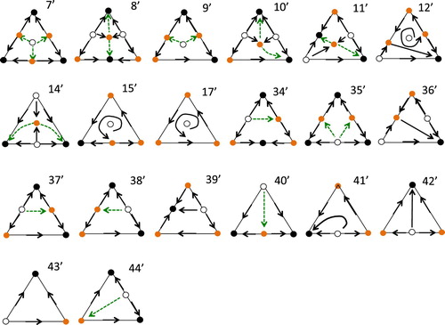
Bomze [3, 4] classified all the possible phase portraits of the 3-species Replicator system. Bomze showed that there are 47 distinct phase portraits up to rotation, reflection and time-reversal. If we leave out non-generic cases where equilibria are not isolated, we reduce the number of possibilities. Moreover, if we ask that all trajectories converge to an equilibrium we can reduce the number of possible portraits yet further to 20, and we depict these possibilities in Figure A1. The cases in Figure A1 must also be considered with their time reversed so that stable nodes become unstable nodes and vice-versa. The numbers used for each phase portrait in Figure A1 match the numbering used by Bomze in [3] and later [4].

In portraits 7, 8, 9, 10, 11, 12, 14, 15, 17 there is a unique interior equilibrium. Of these, in portraits 7, 9, 15, 17 the interior equiilbrium p has $\mathcal{B}\left(p\right)=\text{int}\left(\mathrm{\Delta }\right)$. In 8, 10, 11, 14 there are two asymptotically stable equilibria, say $p_1,p_2$, and the green dashed arrows and the equilibria that they connect make up a continuous curve γ that is the common boundary of the basin of attraction of the two asymptotically stable equilibria. In portrait 12 there are two asymptotically stable equilibria and a heteroclinic orbit joining two boundary equilibria and that forms the common boundary of the basins of attraction of the asymptotically stable equilibria.

For the remaining portraits 34–46 there is no interior equilibrium. In $34,35,37,38,39,40,41,42,43,44$ there is a unique asymptotically stable equilibrium p and $\overline{\mathcal{B}\left(p\right)}=\mathrm{\Delta }$. In portrait 36 there are two asymptotically stable equilibria $p_1,p_2$ on the boundary and the green dashed curve γ toegther with the equilibria that it connects is the common boundary of the attraction basins of $p_1,p_2$.

To comment briefly on two phase portraits in [3] that are not permissible under our assumptions, in both PP 45 and PP 46 of [3, 4] the bottom left vertex is not a hyperbolic equilibrium and so do not satisfy condition (i) of Theorem 2.2.

In Figure A2 we indicate the phase portraits with time reversed with a prime, so that portrait 7' is portrait 7 with time reversed. In 7' there are 3 asymptotically stable equilibria.

Figure A1. Relevant phase portraits for (7(7) $\begin{array}{rl}{\dot{u}}_i& =R{u}_i(u\cdot Au-(Au{)}_i),i=1,2,3.\end{array}$(7) ) when all orbits converge to an equilibrium, and all equilibria are hyperbolic. The asymptotically stable equilbria of the dark solid circles, the saddle equilibria are the orange circles. Finally the hollow circles are unstable nodes. In the cases where there are 2 asymptotically stable equilbria, the dashed green lines are heteroclinic orbits that make up the common boundary of the two attraction basins.

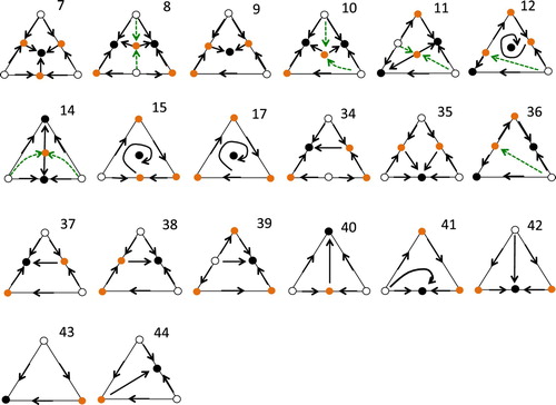
Figure A2. As in Figure A1, but with time reversed. In 7', 15', 35' there are 3 asymptotically stable equilibria. Note that 17' is not relevant as interior points are not convergent, as the omega limit set of the interior equilibrium is $\mathrm{\partial }\mathrm{\Delta }$.

References

- S. Baigent, Geometry of carrying simplices of 3-species competitive Lotka–Volterra systems, Nonlinearity 26 (2013), pp. 1001–1029. doi: 10.1088/0951-7715/26/4/1001
- S. Baigent and Z. Hou, Global stability of interior and boundary fixed points for Lotka–Volterra systems, Differ. Equ. Dyn. Syst. 20 (2012), pp. 53–66. doi: 10.1007/s12591-012-0103-0
- I.M. Bomze, Lotka-Volterra equation and replicator dynamics: A two-dimensional classification, Biol. Cybernet. 48 (1983), pp. 201–211. doi: 10.1007/BF00318088
- I.M. Bomze, Lotka-Volterra equation and replicator dynamics: New issues in classification, Biol. Cybernet. 72 (1995), pp. 447–453. doi: 10.1007/BF00201420
- X. Chen, J. Jiang, and L. Niu, On Lotka–Volterra equations with identical minimal intrinsic growth rate, SIAM J. Appl. Dyn. Syst. 14 (2015), pp. 1558–1599. doi: 10.1137/15M1006878
- C.-W. Chi, L.-I. Wu, and S.-B. Hsu, On the asymmetric May–Leonard model of three competing species, SIAM J. Appl. Math. 58 (1998), pp. 211–226. doi: 10.1137/S0036139994272060
- A. Ching and S. Baigent, Manifolds of balance in planar ecological systems, Appl. Math. Comput.358 (2019), pp. 204–215.
- A. Ching and S. Baigent, The balance simplex in non-competitive 2-species scaled Lotka–Volterra systems, J. Biol. Dyn. 13 (2019), pp. 128–147. doi: 10.1080/17513758.2019.1574033
- L. Gardini, R. Lupini, and M.G. Messia, Hopf bifurcation and transition to chaos in Lotka-Volterra equation, J. Math. Biol. 27(3) (1989), pp. 259–272. doi: 10.1007/BF00275811
- K.P. Hadeler, On copositive matrices, Linear Algebra Appl. 49 (1983), pp. 79–89. doi: 10.1016/0024-3795(83)90095-2
- M.W. Hirsch, Systems of differential equations which are competitive or cooperative: III competing species, Nonlinearity 1 (1988), pp. 51–71. doi: 10.1088/0951-7715/1/1/003
- M.W. Hirsch, On existence and uniqueness of the carrying simplex for competitive dynamical systems, J. Biol. Dyn. 2 (2008), pp. 169–179. doi: 10.1080/17513750801939236
- J. Hofbauer and K. Sigmund, Evolutionary Games and Population Dynamics, Cambridge UP, 1998.
- Z. Hou and S. Baigent, Global stability and repulsion in autonomous Kolmogorov systems, Commun. Pure Appl. Anal. 14 (2015), pp. 1205–1238. doi: 10.3934/cpaa.2015.14.1205
- J. Jiang and L. Niu, On the equivalent classification of three-dimensional competitive Leslie-Gower models via the boundary dynamics on the carrying simplex, J. Math. Biol. 74 (2016), pp. 1–39.
- J. Jiang and L. Niu, On the validity of Zeeman's classification for three dimensional competitive differential equations with linearly determined nullclines, J. Differ. Equ. 263 (2017), pp. 7753–7781. doi: 10.1016/j.jde.2017.08.022
- R. May and W. Leonard, Nonlinear aspects of competition between three species, SIAM J. Appl. Math. 29 (1975), pp. 1–12. doi: 10.1137/0129022
- L. Perko, Differential Equations and Dynamical Systems, Springer Science & Business Media, 2013.
- S. Smale, On the differential equations of species in competition, J. Math. Biol. 3 (1976), pp. 5–7. doi: 10.1007/BF00307854
- Y. Takeuchi, Global Dynamical Properties of Lotka-Volterra Systems, World Scientific, 1996.
- P. Taylor and L. Jonker, Evolutionarily stable strategies and game dynamics, Math. Biosci. 40 (1978), pp. 145–156. doi: 10.1016/0025-5564(78)90077-9
- A. Tineo, May Leonard systems, Nonlinear Anal. Real World Appl. 9 (2008), pp. 1612–1618. doi: 10.1016/j.nonrwa.2007.04.005
- E.C. Zeeman and M.L. Zeeman, From local to global behavior in competitive Lotka-Volterra systems, Trans. Amer. Math. Soc. 355 (2003), pp. 713–734. doi: 10.1090/S0002-9947-02-03103-3
- X.A. Zhang, Z.J. Liang, and L.S. Chen, The global dynamics of a class of vector fields in R3, Acta. Math. Sin. English Ser. 27 (2011), pp. 2469–2480. doi: 10.1007/s10114-011-9053-7