
 ?Mathematical formulae have been encoded as MathML and are displayed in this HTML version using MathJax in order to improve their display. Uncheck the box to turn MathJax off. This feature requires Javascript. Click on a formula to zoom.
Abstract
In this paper, we formulate a stage-structured predator–prey model with mutual interference, in which includes two discrete delays. By theoretical analysis, we establish the stability of the unique positive equilibrium and the existence of Hopf bifurcation when the maturation delay for predators is used as the bifurcation parameter. Our results exhibit that the maturation delay for preys does not affect the stability of the positive equilibrium. However, the maturation delay for predator is able to destabilize the positive equilibrium and causes periodic solutions. Numerical simulations are carried out to illustrate the theoretical results and display the differential impacts of two type delays and mutual interference.
1. Introduction
Since the classical Lotka–Volterra system was proposed, it has been studied by many scholars [Citation1–3,Citation25]. In order to make the model more realistic, some scholars introduce a few concepts to the model, such as mutual interference, stage structure, prey refuge, diffusion and so on [Citation6,Citation10,Citation13,Citation20–22,Citation24,Citation26,Citation27].
The concept of mutual interference was first introduced by Hassell [Citation12] to capture behaviour between a host (a kind of bee) and parasite (a kind of butterfly). It is a measure of the degree of interference between parasites. Furthermore, mutual interference was considered by Freedman [Citation8,Citation9] to describe a phenomenon that predators have the tendency to leave each other when they met. In [Citation8] Freedman proposed a general Volterra model with mutual interference as follows,
(1)
(1) where
,
,
(for some K),
,
,
,
. In the special case of m = 1, the above system reduces to the traditional predator–prey model.
In nature, the predatory behaviour and reproduction behaviour are mainly completed by adult individuals and these abilities for juvenile can be ignored, and the birth rate and death rate in species' whole life history are obviously different. Based on this facts mentioned above, the population exhibit two distinct stages: immature and mature. It leads to the stage-structured model with delay representing the time from birth to maturity. Aiello and Freedman [Citation4] proposed the following stage-structured single species model
(2)
(2) where
is the immature population densities and mature population densities, respectively. r>0 represents the birth rate, d>0 is the immature death rate, b>0 is the mature death and overcrowding rate, τ is the time from birth to maturity. The term
represents those immatures who were born at time
and survive at time t (with the immature death rate d), and exit from the immature population and enter the mature population.
Many scholars used the idea of Aiello and Freedman to establish stage-structured predator–prey models [Citation6,Citation19,Citation27]. Recently, Li et al. [Citation19] proposed and investigated an autonomous predator–prey system with stage structure and mutual interference. The model is given as follows
(3)
(3) where
,
and
represent the densities of immature prey, mature prey and predator, respectively. m with 0<m<1 is the mutual interference constant.
is the birth rate of mature prey, d is the death rate of the immature prey,
is the surviving rate of each immature prey to reach maturity, τ is the maturation delay for prey,
is the self regulation constant of the prey,
represents the capturing rate of predator;
is the intrinsic death rate of predator,
denote the intra-specific competition among the predator,
denotes the conversion rate for the predator. Model (Equation3
(3)
(3) ) only consider the stage structure in prey. The dynamical behaviour of (Equation3
(3)
(3) ) are established in [Citation19]. Furthermore, Huang and Dong [Citation17] improve the related results that the interior equilibrium of (Equation3
(3)
(3) ) is always globally asymptotically stable without any additional conditions.
Another problem that attracts us and can not be ignored is the influence of the maturation delay for predator. Actually, there is a big difference between mature predator and immature predator in their survival habits, for example, birth rate, death rate, the ability to feed on and reproduce [Citation27]. In the present paper, in order to study the combined effects of stage structures for prey along with predator and mutual interference, we consider the following delayed predator–prey model,
(4)
(4) where
and
represent the densities of immature and mature prey, and
and
denote the densities of the immature and mature predator, respectively. m,
,
,
,
,
,
,
,
are positive constants, the parameters
,
,
,
are defined in model (1.3).
is the capturing rate of mature predators,
describes the rate of conversion of nutrients into the reproduction rate of the mature predators,
is the death rate of immature predators,
denotes the maturation delay for predator [Citation14], the term
stands for the number of immature predator that were born at time
which still survive at time t and are transferred from the immature stage to the mature stage at time t,
is the death rate of mature predator,
denotes the intra-specific competition among the mature predator. It is assumed that the mature individual predator only feeds on the mature preys and the immature individual predator have no competence to feed on mature prey and reproduce.
For biological meaning, the initial conditions for system (Equation4(4)
(4) ) take the form
(5)
(5) where
. For the continuity of the solution of system (Equation4
(4)
(4) ), intergrating both sides of the first equation and the third equation of (Equation4
(4)
(4) ) on
, we have
(6)
(6) and
The equations above mean that and
could be decided by
and
, respectively. For simplicity, here we rewrite
and
as
and
. We investigate the asymptotical behaviour for the subsystem of system (Equation4
(4)
(4) ) as follows,
(7)
(7) with the initial conditions as follows,
(8)
(8)
Denote , the Banach space of continuous functions mapping the interval
into
, where we define
Although the dynamical behaviours of the stage-structured species has been well studied by DDE models (see [Citation19,Citation22–27]), most of them considered only the effect of maturation delay in prey or predator, separately. Model (Equation7(7)
(7) ) includes two types of delay simultaneously. The aim of the present paper is to carry out mathematical analysis of system (Equation7
(7)
(7) ) and to find out the different influences of maturation delay for prey, maturation delay for predator, and mutual interference. We are interested in whether the prey and predator are always persistent, and whether the ecological system approaches an equilibrium or it varies periodically.
The organization of this paper is as follows. In Section 2, we introduce some useful lemmas and propositions. In Section 3, we analyse the stability of the boundary equilibria of system (Equation7(7)
(7) ). In Section 4, we study the dynamics properties of the positive equilibrium of system (Equation7
(7)
(7) ). In Section 5, we give detailed numerical simulations to verify our theoretical analysis above. In the last section, we give a brief discussion.
2. Preliminaries
In the following we will give some propositions and some useful lemmas.
Proposition 2.1
The solutions of the system (Equation7
(7)
(7) ) are positive under the initial conditions (Equation8
(8)
(8) ).
Proof.
Assume, by way of contradiction, does not hold. There must exist
such that
. Set
We know
, and
. From (Equation7
(7)
(7) ), we have
(9)
(9) which is a contradiction to the fact that
. Hence
holds. In a similar way we can proof
.
The proof is completed.
Lemma 2.1
[Citation21]
Consider the following equation:
and assume that
and
. Then
Lemma 2.2
[Citation7]
Assume that a>0, b>0, ,
and
. Then
Next, we prove the boundedness of the solutions of system (Equation7(7)
(7) ).
Proposition 2.2
The solutions of system (Equation7(7)
(7) ) are bounded for all large t.
Proof.
From the first equation of (Equation7(7)
(7) ), we have
(10)
(10) According to Lemma 2.1, we have
(11)
(11) There is
and
such that
(12)
(12) Now, we show that
is bounded. By a contradiction, we assume that
is boundless. Because of the continuity of the system, there is
such that
(13)
(13) By the second equation of (Equation5
(5)
(5) ) and (Equation13
(13)
(13) ), we get
(14)
(14) According to Lemma 2.1, we have
(15)
(15) which is a contradiction to the assumption. Hence
is bounded. Therefore,
and
are both bounded.
The proof is completed.
System (Equation7(7)
(7) ) always has two boundary equilibria, which are
and
. Besides, we will prove the existence of the positive equilibrium of system (Equation7
(7)
(7) ) as follows.
Proposition 2.3
System (Equation7(7)
(7) ) always has a unique positive equilibrium
.
Proof.
satisfies the following equations,
(16)
(16) Noting that
is not the solution of (Equation16
(16)
(16) ). We can rewrite (Equation16
(16)
(16) ) as another form,
(17)
(17) Define
and
as following forms:
(18)
(18) By simple computations, we have
,
,
,
, which is easy to know that
is a monotony decrease function, namely
;
and
. Therefore,
is a convex function and
is an increase function for y>0.
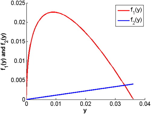
From above analysis, it follows that both curves of (Equation18(18)
(18) ) have unique intersection for y>0 (see Figure ).
Figure 1. The curves of and
.
In the following we discuss the the uniform permanence of system (Equation7(7)
(7) ).
Proposition 2.4
If , where
, the system (Equation7
(7)
(7) ) with initial conditions (Equation8
(8)
(8) ) is permanent. That is, for any positive solution
of system (Equation7
(7)
(7) ), one has
Proof.
According to Proposition 2.2, we have . Then from the second equation of system (Equation7
(7)
(7) ), we have
(19)
(19) According to Lemma 2.2, we have
(20)
(20) Then combine the above inequation and the first equation of system (Equation7
(7)
(7) ), we have
(21)
(21) By the Lemma 2.1, we have
(22)
(22) Then combine the above inequation and the second equation of system (Equation7
(7)
(7) ), we have
(23)
(23) Thus, by the Lemma 2.2, we have
(24)
(24) The proof is completed.
3. Stability analysis for two boundary equilibria
In order to investigate the stability of the equilibria of system (Equation7(7)
(7) ), we linearize the system and obtain the characteristic equation evaluated at an equilibrium
, given by the following formula,
(25)
(25) where λ is an eigenvalue and
We first discuss the stability of two boundary equilibria.
Theorem 3.1
The equilibrium of system (Equation7
(7)
(7) ) is unstable for any
.
Proof.
From (Equation25(25)
(25) ), we know that y = 0 is meaningless, so
cannot be substituted into (Equation25
(25)
(25) ).
By using the method in [Citation23], we set
For
, the characteristic equation is given by
(26)
(26) The characteristic equation have a eigenvalue
and another derived by
. It is easy to know that it exist
and
from the fact that
and
, so the equilibrium
is unstable.
The proof is completed.
Theorem 3.2
The equilibrium of system (Equation7
(7)
(7) ) is unstable for any
.
Proof.
For , noting that
makes no sense, hence the local stability of
cannot be investigated by computing the Jacobian matrix directly. We will study it by investigating the exceptional direction and normal sector of the equilibrium.
Firstly, is unstable and
are orbits. y = 0 is along the x-axis into the orbit of
from Lemma 2.1. For 0<m<1, we denote
, then n>1. By using the following change of variables
and rewriting
as x, y, t, we obtain another form of system (Equation7
(7)
(7) ),
(27)
(27) Then the equilibrium
is high order singular point. Thus we translate the point
to the original
. By letting
,
and rewriting
as x, y, we obtain another form of system (Equation27
(27)
(27) ),
(28)
(28) Let
,
, system (Equation28
(28)
(28) ) can be rewritten as the following equation of polar coordinates:
(29)
(29) where
(30)
(30) Obviously,
and
are exceptional directions. Noting that
,
and
,
, hence the normal sectors of
and
are of second type and there is a unique orbit which is along the exceptional direction
and
into the equilibrium
of (Equation28
(28)
(28) ). That is, there is a unique orbit of system (Equation7
(7)
(7) ) in
along the line
into
. On the other hand, since
(31)
(31) it implies that the orbit of system (Equation7
(7)
(7) ) intersecting with the line
passes through the right into the left. Hence the equilibrium
is unstable.
The proof is completed.
The two bounded equilibria are all unstable and system (Equation7(7)
(7) ) is bounded and positive with the initial conditions (Equation8
(8)
(8) ), which mean that system is persistent. In fact, in an ecological model consisting of predators and preys, if the predator's predation ability is very strong, the population of predator and prey maybe tend to die out. While if there are mutual interference in the predator, the population of predator and prey will be persistence. In the next section, we mainly study the dynamical properties of the positive equilibrium. In other word, on the basic of the fact that predator and prey will be persistence, how do the two maturation time delays for predator and prey affect the population of predator and prey, whether the population of two species tends to a stable steady state or presents a periodic obit.
4. Dynamical analysis for the positive equilibrium
System (Equation7(7)
(7) ) always has a unique positive equilibrium
. Now we study the dynamical properties of the positive equilibrium of system (Equation7
(7)
(7) ) in three cases: (I)
; (II)
,
; (III)
,
.
Case (I) where .
In the case where there is no maturation delay for both prey and predator, (Equation7(7)
(7) ) is reduced to the following ordinary differential equations model,
(32)
(32) System (Equation32
(32)
(32) ) has the same equilibria as system (Equation7
(7)
(7) ) and the boundary equilibria are also unstable. The characteristic equation of system (Equation32
(32)
(32) ) at
is as follows,
(33)
(33) where
It follows from the Routh-Hurwitz criteria that all roots of (Equation33
(33)
(33) ) only have negative real roots. It means that the positive equilibrium
is locally asymptotically stable.
Next, by using the similar Lyapunov function in [Citation15,Citation16], we could establish the global stability of of system (Equation32
(32)
(32) ).
Define a function,
Since
, we have
Here we use
, then we have
For 0<m<1, since
(34)
(34) it follows that the positive-define function
has non-positive derivative
. Let
be the largest invariant subset of
. Now we define
. Since
equals to zero if and only if
,
, we see that
is the singleton
. By the LaSalle invariance principle [Citation11], every solution of (Equation32
(32)
(32) ) tends to the positive equilibrium
, which is globally asymptotically stable.
According to above theoretical analysis, we have the following theorem.
Theorem 4.1
For , the positive equilibrium
of system (Equation7
(7)
(7) ) is globally asymptotically stable.
Case (II) where ,
.
In the case where there is no maturation delay for predator, system (Equation7(7)
(7) ) is reduced to a delay differential equations model which includes one maturation delay for prey as follows,
(35)
(35)
As a special case of (Equation7(7)
(7) ), the complete global stability of (Equation35
(35)
(35) ) was established by Huang and Dong in [Citation17].
Theorem 4.2
[Citation17]
For ,
, the positive equilibrium
of system (Equation7
(7)
(7) ) is globally asymptotically stable for any delay
.
Case (III) where ,
.
In the case where there is no maturation delay for prey, system (Equation7(7)
(7) ) includes one maturation delay for predator as follows,
(36)
(36) System (Equation36
(36)
(36) ) has the same equilibria as system (Equation7
(7)
(7) ) and the boundary equilibria are also unstable. The characteristic equation of system (Equation36
(36)
(36) ) at the positive equilibrium
is as follows,
(37)
(37) whose coefficients are
We note that, if
, these coefficients are dependant on the delay
, since
and
all include
. From case (I), we know that the positive equilibrium
is locally asymptotically stable when
. Then, we let
vary and investigate the possible bifurcations. For
to become unstable, characteristic roots have to cross the imaginary axis to the right when
increases and
can not be a root of (Equation37
(37)
(37) ) since that
Let
be a purely imaginary root of (Equation37
(37)
(37) ). Substituting it into (Equation37
(37)
(37) ) and separating the real and imaginary parts, we obtain
(38)
(38) Squaring and adding both equations of (Equation38
(38)
(38) ) lead to
(39)
(39) where
A root
of (Equation37
(37)
(37) ) satisfying
if and only if
. Because of
,
is equivalent to
According to above theoretical analysis, we have the following theorem.
Theorem 4.3
If holds, then
has the positive roots
for
.
Let be a positive root of
. For
to be a solution of (Equation37
(37)
(37) ),
needs to satisfy the system
(40)
(40) Define
(41)
(41) and let
and
be the solution of (Equation41
(41)
(41) ).
Following the methods proposed by Beretta and Kuang [Citation5], we set
(42)
(42) Then
are purely imaginary roots of (Equation37
(37)
(37) ) if and only if
is a zero of function
for some
.
Following from the following equality
and the fact that
we have the following theorem.
Theorem 4.4
Assume that the function has a positive root
for some
, then a pair of simple purely imaginary roots
of (Equation37
(37)
(37) ) exist at
and
Furthermore, the pair of simple purely imaginary roots
cross the imaginary axis to the right at
if
.
Be similar to [Citation18], the following properties of can be verified using (Equation42
(42)
(42) ).
,
Let
When
From the properties (ii) and (iii) we know that and if
has a positive zero, then
necessarily has at least two positive zeros in
. Assume that
has two positive zeros
, with
and
. A pair of complex conjugate eigenvalues cross the imaginary axis to the right at
, remain to the right for
and cross back to the right at
. Accordingly,
remains stable for
, loses its stability for
and regains its stability for
. This is the stability switch phenomenon. In Figure , we show that solutions converge to the stable
for
, and that solutions converge to a stable periodic solutions for
. According to above theoretical analysis, we have the theorems as follows.
Theorem 4.5
If does not hold or
holds but that
has no positive zeros, no Hopf bifurcation occurs and the interior equilibrium
remains locally asymptotically stable for all
.
Theorem 4.6
If holds and that
,
, have positive simple zeros,
, system (Equation7
(7)
(7) ) undergoes a Hopf bifurcation at the equilibrium
when
, i = 1, m. The Hopf bifurcation is supercritical at
and subcritical at
. Furthermore,
goes through stability switches:
is asymptotically stable for
, and unstable when
.
5. Numerical simulations
Here we perform numerical simulations to verify the above theoretical analysis results. Moreover, we would verify the stability switches as shown in Section 4 and find dynamical behaviour of (Equation7(7)
(7) ) when two delays are present simultaneously.
Firstly, we choose a set of parameter values except for and
as follows
(43)
(43) From Theorems 4.1 and 4.2, when we only consider the stage structure in prey and ignore the stage structure in predator, the positive (coexistence) equilibrium is always globally asymptotically stable. Actually, the maturation delay for prey does not affect the stability of the system. However, since the curve of
will move down with the increase of
, the value of x-axis of the intersection of
and
will decrease. It means that the values of
and
all decrease as the increase of
. For biological meaning, this means that longer juvenile maturation for prey leads to both populations decrease of predator and prey when they are in the stable steady state. We give simulations to present the impact of the maturation delay for prey in model (Equation7
(7)
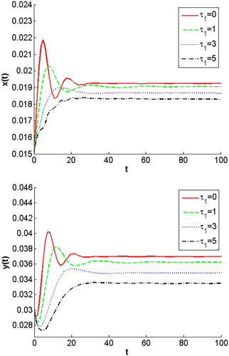
(7) ). We fix m = 0.5,
and vary
, which correspond to four values of
. Figure show that all solutions converge to the equilibrium
with small oscillation and the values of
and
decrease as the increase of
.
Figure 2. All solutions converge to the positive equilibrium for different
. Here we fix m = 0.5,
and choose the other parameters from (Equation43
(43)
(43) ) and the initial value is
.
Second, we fix and vary the values of m and
, respectively. The stability region of the unique positive equilibrium
and Hopf bifurcation curve in the
parameter plane are given in Figure . The area below the curve represents the regions of stability of
and the area above the curve represents the regions of instability of
. In Figure , we could observe that the value of
decreases as the increase of m, which means the critical value of
that change the stability of
of system (Equation36
(36)
(36) ) decreasing as the value of m increases. Similarly, we can see that the value of m decrease as the increase of
, which means the critical value of
that change the stability of
of system (Equation36
(36)
(36) ) decreasing as the value of
increases. For biological meanings, the maturation delay for predator and mutual interference also determine the final state of the ecosystem consisting of predators and preys. The next, we choose two special values to observe the Hopf bifurcation branches and the time evolution curves of system (Equation36
(36)
(36) ). When we choose m = 0.5, the value
of bifurcation curve is about 1.545 (see Figure ). This means that the positive equilibrium
of system (Equation32
(32)
(32) ) can become unstable by choose some appropriate values
. For example, if we choose
, the positive equilibrium
is stable (see Figure (a)); if we choose
, the positive equilibrium
becomes unstable and a stable periodic solution with a simple shape appears (see Figure (b)); if we choose
, the positive equilibrium
is still unstable but a stable periodic solution with a complex shape appears (see Figure (c)). Corresponding solution curves can be seen in Figure (e,f). In fact, the positive equilibrium
will eventually become stable (see Figure (d), we choose
). When we choose
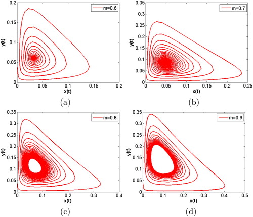
, the value m of bifurcation curve is about 0.777 (see Figure ). This means that the stability of
will change at the value m = 0.777. For example, if we choose m = 0.6, 0.7,
is stable (see Figure (a,b)); if we choose m = 0.8, 0.9,
becomes unstable and a stable periodic solution with a simple shape appears (see Figure (c,d)).
Figure 3. Hopf bifurcation curves in the parameter plane.
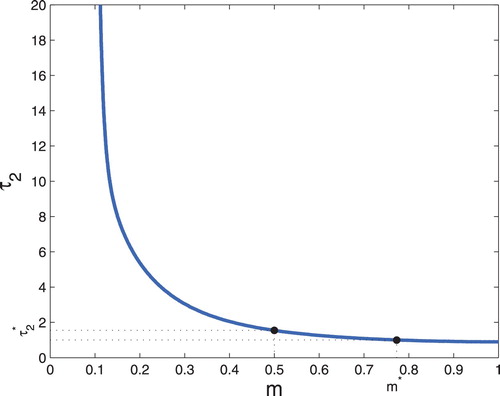
Figure 4. Hopf bifurcation branches are computed when we vary and keep m = 0.5. The positive equilibrium
goes through stability switches at
.
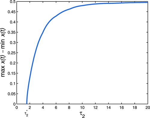
Figure 5. Hopf bifurcation branches are computed when we vary m and keep . The positive equilibrium
goes through stability switches at
.
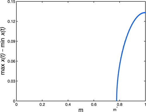
Figure 6. m = 0.5 is fixed. The time evolution curves of system (Equation35(35)
(35) ) corresponding to four values
. (a) It shows that when
, the solutions of system tend to the equilibrium
; (b) it shows that when
, a stable periodic solution with a simple shape appears; (c) it shows that when
, a stable periodic solution with a complex shape appears; (d) it shows that when
, the solutions of system tend to the equilibrium
again. (e) and (f) show the time evolution curves of
and
when
, respectively.
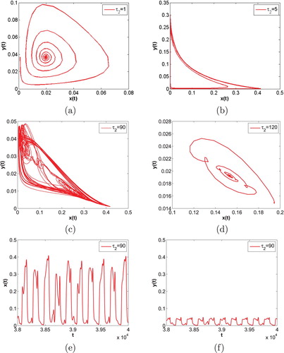
Figure 7. is fixed. The time evolution curves of system (Equation35
(35)
(35) ) corresponding to four values m = 0.6, 0.7, 0.8, 0.9. (a) and (b) show that when
, the solutions of system tend to the equilibrium
; (c) and (d) show that when
, a stable periodic solutions with a simple shape appears.
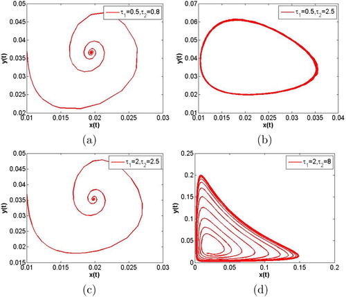
Finally, we fix m = 0.5 and vary the values of and
to observe the joint effect of
and
on a stable system (see Figure (a)). When we choose
, the solution of system (Equation7
(7)
(7) ) tend to the equilibrium
(see Figure (a)); when we choose
,
, a stable periodic solutions appear (see Figure (b)); When we choose
,
, the solution of system (Equation7
(7)
(7) ) tend to the equilibrium
again (see Figure (c)); when we choose
,
, a stable periodic solutions appears again (see Figure (d)). Comparing Figure (a,b), we can easily find out the fact that the system (Equation7
(7)
(7) ) will be unstable as the increase of
when
is fixed, which is similar to Figure (a,b). While we increase the value of
and fix the value of
, the system (Equation7
(7)
(7) ) becomes locally stability again (see Figure (c)). Comparing Figure (c,d), we can easily find out that the stability of system (Equation7
(7)
(7) ) switches again as the augment of
. The above numerical simulation shows that the augment of
will increase the critical value
changing the stability of
of system (Equation7
(7)
(7) ). In other words, when the population of predator is changing periodically, we can let the population of predator in a stable steady state by increasing the maturation delay for prey.
Figure 8. m = 0.5 is fixed. The time evolution curves of system (Equation7(7)
(7) ). (a) When
, the solutions of system tend to the equilibrium
. (b) Compared with (a), when we vary
and fix
, a stable periodic solution with a simple shape appears. (c) Compared with (b), when we vary
and fix
, the solutions of system tend to the equilibrium
again, which shows that the augment of
increases the switch value
(d) When
, a stable periodic solution with a simple shape appears again.
6. Discussion
In this paper, a class of more general and realistic stage-structured predator–prey model is developed and analysed. The model includes mutual interference and two maturation delays. The maturation time for prey does not effect the globally asymptotically stable, but the maturation time for predator may lead to the model undergo Hopf bifurcation. When maturation time for predator is small, the positive equilibrium is locally asymptotically stable; when
increases, the positive equilibrium is unstable and it brings the periodic solutions; when
is large enough, the positive equilibrium recovers locally asymptotically stable. The analysis in this paper helps us to understand how delays affect the Lotka–Volterra predator–prey system. Biologically, the theoretical and numeric analysis are also useful to explain that the population of animals raised (or hatched) longer or smaller will be in a stable state. At the same time, the length of incubation has little effect on the dynamics of predator.
Another problem interested us is that the system always has a unique positive equilibrium and the bounded equilibria are always unstable owe to the existence of mutual interference , in other words, the system is always persistent without any additional conditions. In most Lotka–Volterra predator–prey models, only under some addition conditions will the bounded equilibria be unstable. As the special case where m = 1 (that is, no mutual interference), the positive equilibrium of the system is stable if and only if the condition
holds. From the biological viewpoint, it means that the mutual interference
helps the endangered predators survive. The possible reason is that the strength of predation of predators declines sharply causing that the population of prey remain in a relatively high level.
Disclosure statement
No potential conflict of interest was reported by the author(s).
Additional information
Funding
References
- S. Ahmad, On the nonautonomous Volterra-Lotka competition equations, Proc. Amer. Math. Soc. 117 (1993), pp. 199–204. doi: 10.1090/S0002-9939-1993-1143013-3
- S. Ahmad, Extinction of species in nonautonomous Lotka-Volterra systems, Proc. Amer. Math. Soc. 127 (1999), pp. 2905–2910. doi: 10.1090/S0002-9939-99-05083-2
- S. Ahmad and A.C. Lazer, Average conditions for global asymptotic stability in a nonautonomous Lotka-Volterra system, Nonlinear Anal. Theor. Meth. Appl. 40 (2000), pp. 37–49. doi: 10.1016/S0362-546X(00)85003-8
- W.G. Aiello and H.I. Freedman, A time-delay model of single-species growth with stage structure, Math. Biosci. 101 (1990), pp. 139–153. doi: 10.1016/0025-5564(90)90019-U
- E. Beretta and Y. Kuang, Geometric stability switch criteria in delay differential systems with delay dependent parameters, SIAM J. Math. Anal. 33 (2002), pp. 1144–1165. doi: 10.1137/S0036141000376086
- F. Chen, X. Xie, and J. Shi, Existence, uniqueness and stability of positive periodic solution for a nonlinear prey-competition model with delays, J. Comput. Appl. Math. 194 (2006), pp. 368–387. doi: 10.1016/j.cam.2005.08.005
- F. Chen, Z. Li, and X. Xie, Permanence of a nonlinear integro-differential prey-competition model with infinite delays, Commun. Nonlinear Sci. Numer. Simul. 13 (2008), pp. 2290–2297. doi: 10.1016/j.cnsns.2007.05.022
- H.I. Freedman, Stability analysis of a predator-prey system with mutual interference and density-dependent death rates, Bull. Math. Biol. 41 (1979), pp. 67–78. doi: 10.1016/S0092-8240(79)80054-3
- H.I. Freedman and V.S. Rao, The trade-off between mutual interference and time lags in predator-prey systems, Bull. Math. Biol. 45 (1983), pp. 991–1004. doi: 10.1016/S0092-8240(83)80073-1
- G. Guo and J. Wu, The effect of mutual interference between predators on a predator-prey model with diffusion, J. Math. Anal. Appl. 389 (2012), pp. 179–194. doi: 10.1016/j.jmaa.2011.11.044
- J. Hale and S.M. Verduyn Lunel, Introduction to Functional Differential Equations, Applied Mathematical Science, Vol. 9, New York, 1993.
- M.P. Hassell, Mutual interference between searching insect parasites, J. Anim. Ecol. 40 (1971), pp. 473–486. doi: 10.2307/3256
- H. Hu and L. Huang, Stability and Hopf bifurcation in a delayed predator–prey system with stage structure for prey, Nonlinear Anal. Real World Appl. 11 (2010), pp. 2757–2769. doi: 10.1016/j.nonrwa.2009.10.001
- C. Huang, Y. Qiao, L. Huang, and R. Agarwal, Dynamical behaviors of a food-chain model with stage structure and time delays, Adv. Differ. Equ. 2018 (2018), pp. 1–26. doi: 10.1186/s13662-017-1452-3
- G. Huang, Y. Takeuchi, and R. Miyazaki, Stability conditions for a class of delay differential equations in single species dynamics, Discrete Contin. Dyn. Syst. B 17 (2012), pp. 2451–2464. doi: 10.3934/dcdsb.2012.17.2451
- G. Huang, A. Liu, and U. Forys, Global stability analysis of some nonlinear delay differential equations in population dynamics, J. Nonlinear Sci. 26 (2016), pp. 27–41. doi: 10.1007/s00332-015-9267-4
- G. Huang, Y. Dong, A note on global properties for a stage structured predator-prey model with mutual interference. Adv. Differ. Equ. 308 (2018), pp. 1–10. doi:10.1186/s13662-018-1767-8
- M. Y. Li and H. Shu, Joint effects of mitosis and intracellular delay on viral dynamics: Two-parameter bifurcation analysis, J. Math. Biol. 64 (2012), pp. 1005–1020. doi: 10.1007/s00285-011-0436-2
- Z. Li, M. Han, and F. Chen, Global stability of a predator-prey system with age-struture and mutual interference, Discrete Contin. Dyn. Syst. B 19 (2014), pp. 173–187. doi: 10.3934/dcdsb.2014.19.173
- S. Liu, L. Chen, G. Luo, and Y. Jiang, Asymptotic behaviors of competitive Lotka-Volterra system with stage structure, J. Math. Anal. Appl. 271 (2002), pp. 124–138. doi: 10.1016/S0022-247X(02)00103-8
- S. Liu, L. Chen, and Z. Liu, Extinction and permanence in nonautonomous competitive system with stage structure, J. Math. Anal. Appl. 274 (2002), pp. 667–684. doi: 10.1016/S0022-247X(02)00329-3
- Y. Lu, K.A. Pawelek, and S. Liu, A stage-structured predator-prey model with predation over juvenile prey, Appl. Math. Comput. 297 (2017), pp. 115–130.
- Z. Ma, F. Chen, C. Wu, and W. Chen, Dynamic behaviors of a Lotka-Volterra predator-prey model incorporating a prey refuge and predator mutual interference, Appl. Math. Comput. 219 (2013), pp. 7945–7953.
- K. Wang, Permanence and global asymptotical stability of a predator–prey model with mutual interference, Nonlinear Anal. Real World Appl. 12 (2011), pp. 1062–1071. doi: 10.1016/j.nonrwa.2010.08.028
- X. Wang, Z. Du, and J. Liang, Existence and global attractivity of positive periodic solution to a Lotka-Volterra model, Nonlinear Anal. Real World Appl. 11 (2010), pp. 4054–4061. doi: 10.1016/j.nonrwa.2010.03.011
- R. Xu, Global dynamics of a predator–prey model with time delay and stage structure for the prey, Nonlinear Anal. Real World Appl. 12 (2011), pp. 2151–2162. doi: 10.1016/j.nonrwa.2010.12.029
- R. Xu, M.A.J Chaplain, and F.A. Davidson, Persistence and stability of a stage-structured predator-prey model with time delays, Appl. Math. Comput. 150 (2004), pp. 259–277.