Chaotic attractors in Atkinson–Allen model of four competing species

Abstract

We study the occurrence of chaos in the Atkinson–Allen model of four competing species, which plays the role as a discrete-time Lotka–Volterra-type model. We show that in this model chaos can be generated by a cascade of quasiperiod-doubling bifurcations starting from a supercritical Neimark–Sacker bifurcation of the unique positive fixed point. The chaotic attractor is contained in a globally attracting invariant manifold of codimension one, known as the carrying simplex. Biologically, our study implies that the invasion attempts by an invader into a trimorphic population under Atkinson–Allen dynamics can lead to chaos.

Keywords:

• Atkinson–Allen model
• carrying simplex
• Neimark–Sacker bifurcation
• quasiperiod-doubling bifurcation
• chaotic attractor
• invasion

1. Introduction

Consider the discrete-time Atkinson–Allen model of n mutually competing species induced by the map (1) $T_i(x)=\frac{(1+s_i)(1-c_i)x_i}{1+\sum _{j=1}^n{b}_{ij}{x}_j}+c_i{x}_i,0<c_i<1,b_{ij},s_i>0,i,j=1,\dots ,n$(1) on ${\mathbb{R}}_{+}^n=[0,\mathrm{\infty }{)}^n$, where $x=(x_1,\dots ,x_n{)}^{\tau }$ is the vector of populations at one generation, and $T(x)=(T_1(x),\dots ,T_n(x){)}^{\tau }$ is the corresponding vector at the next generation. Parameter $b_{ii}$ is the rate of intraspecific competition of the species i; parameter $b_{ij}(i\ne j)$ is the rate of interspecific competition of the species j on the species i; and parameter $c_i$ is the survival rate of the species i from one generation to the next generation. We refer the reader to [15] for the mechanistic derivation of the Atkinson–Allen model (1(1) $T_i(x)=\frac{(1+s_i)(1-c_i)x_i}{1+\sum _{j=1}^n{b}_{ij}{x}_j}+c_i{x}_i,0<c_i<1,b_{ij},s_i>0,i,j=1,\dots ,n$(1) ) from first principles. The Atkinson–Allen model (1(1) $T_i(x)=\frac{(1+s_i)(1-c_i)x_i}{1+\sum _{j=1}^n{b}_{ij}{x}_j}+c_i{x}_i,0<c_i<1,b_{ij},s_i>0,i,j=1,\dots ,n$(1) ) plays a role as a discretized system of the classical continuous-time Lotka–Volterra model of competition (see [15,29]) (2) $\frac{\mathrm{d}{x}_i(t)}{\mathrm{d}t}=x_i(t)({\xi }_i-\sum _{j=1}^n{\alpha }_{ij}{x}_j(t)),{\xi }_i,{\alpha }_{ij}>0,i,j=1,\dots ,n.$(2) The Atkinson–Allen map T given by (1(1) $T_i(x)=\frac{(1+s_i)(1-c_i)x_i}{1+\sum _{j=1}^n{b}_{ij}{x}_j}+c_i{x}_i,0<c_i<1,b_{ij},s_i>0,i,j=1,\dots ,n$(1) ) is unbounded but invertible on ${\mathbb{R}}_{+}^n$ which admits a carrying simplex $\mathrm{\Sigma }\subset {\mathbb{R}}_{+}^n\setminus \{0\}$, that is an invariant hypersurface of codimension one, which attracts all non-trivial orbits (see [15]). The origin 0 is a repeller for T, and Σ is the boundary in ${\mathbb{R}}_{+}^n$ of the basin of repulsion of the origin which satisfies the following properties:

• Σ is compact and unordered, i.e. if $x,z\in \mathrm{\Sigma }$ such that $x_i\ge z_i$ for all $i=1,\dots ,n$, then x = z;

• Σ is homeomorphic via radial projection to the $(n-1)$-dimensional standard probability simplex ${\mathrm{\Delta }}^{n-1}=\{x\in {\mathbb{R}}_{+}^n:\sum _{i=1}^n{x}_i=1\}$;

• $\mathrm{\forall }x\in {\mathbb{R}}_{+}^n\setminus \{0\}$, there is some $z\in \mathrm{\Sigma }$ such that ${\displaystyle \underset{k\to \mathrm{\infty }}{lim}|T^k(x)-T^k(z)|=0}$;

• $T(\mathrm{\Sigma })=\mathrm{\Sigma }$, and $T:\mathrm{\Sigma }\mapsto \mathrm{\Sigma }$ is a homeomorphism.

The importance of the existence of a carrying simplex Σ stems from the fact that Σ captures the relevant long-term dynamics. In particular, it contains all non-trivial fixed points, periodic orbits, invariant circles and heteroclinic cycles (see, for example, [15,20,21,23]).

The dynamical behaviour of the Atkinson–Allen model (1(1) $T_i(x)=\frac{(1+s_i)(1-c_i)x_i}{1+\sum _{j=1}^n{b}_{ij}{x}_j}+c_i{x}_i,0<c_i<1,b_{ij},s_i>0,i,j=1,\dots ,n$(1) ) for single species is trivial, that is every nonzero trajectory tends to the positive fixed point because it is a strictly increasing map on ${\mathbb{R}}_{+}$. The Atkinson–Allen model (1(1) $T_i(x)=\frac{(1+s_i)(1-c_i)x_i}{1+\sum _{j=1}^n{b}_{ij}{x}_j}+c_i{x}_i,0<c_i<1,b_{ij},s_i>0,i,j=1,\dots ,n$(1) ) of two competing species also only has trivial dynamics, that is every trajectory converges to a fixed point due to the existence of a one-dimensional carrying simplex; see [15,32]. The Atkinson–Allen model (1(1) $T_i(x)=\frac{(1+s_i)(1-c_i)x_i}{1+\sum _{j=1}^n{b}_{ij}{x}_j}+c_i{x}_i,0<c_i<1,b_{ij},s_i>0,i,j=1,\dots ,n$(1) ) of three competing species has much richer dynamics (see [5,15,20,28,29]). In particular, Gyllenberg et al. classified the three-dimensional model (1(1) $T_i(x)=\frac{(1+s_i)(1-c_i)x_i}{1+\sum _{j=1}^n{b}_{ij}{x}_j}+c_i{x}_i,0<c_i<1,b_{ij},s_i>0,i,j=1,\dots ,n$(1) ) in terms of inequalities on the parameters via the boundary dynamics on the two-dimensional carrying simplex in [15], and derived a total of 33 stable equivalence classes. They found that non-trivial dynamics, such as Neimark–Sacker bifurcations and heteroclinic cycles can occur in some classes. The Neimark–Sacker bifurcation is a well-known phenomenon occurs for a discrete-time dynamical system in two or more dimensions induced by a smooth map depending on a parameter, $\mu \in \mathbb{R}$ say, with a fixed point $x^{\ast }(\mu )$ whose Jacobian has a pair of complex conjugate eigenvalues $\lambda (\mu ),\overline{\lambda }(\mu )$ which cross the unit circle transversally at $\mu =0$; i.e., $r(\mu )=|\lambda (\mu )|$ satisfies $r(0)=1,r^{\mathrm{\prime }}(0)\ne 0$, and then, generically, as μ passes through $\mu =0$, the fixed point $x^{\ast }(\mu )$ changes stability and a unique invariant circle bifurcates from it; see [24,27,31]. Moreover, either all orbits are periodic, or all orbits are dense on such an invariant circle (in this case, we call the invariant circle a quasiperiodic curve). However, it was proved that in classes 1−25 and 33, every nonzero trajectory converges to a fixed point on the carrying simplex, that is the dynamics in these classes is trivial; see [3,15,16,28]). Their results show that the three-dimensional Atkinson–Allen model (1(1) $T_i(x)=\frac{(1+s_i)(1-c_i)x_i}{1+\sum _{j=1}^n{b}_{ij}{x}_j}+c_i{x}_i,0<c_i<1,b_{ij},s_i>0,i,j=1,\dots ,n$(1) ) has the similar dynamic scenarios as the Lotka–Volterra competitive model (2(2) $\frac{\mathrm{d}{x}_i(t)}{\mathrm{d}t}=x_i(t)({\xi }_i-\sum _{j=1}^n{\alpha }_{ij}{x}_j(t)),{\xi }_i,{\alpha }_{ij}>0,i,j=1,\dots ,n.$(2) ); see [34,39]. The reader can consult, for instance, [1,2,4,17,22,26,36–38], for more results on the Lotka–Volterra competitive model.

Note that there is a two-dimensional carrying simplex Σ for the three-dimensional continuous flow ψ induced by a totally competitive system of ODEs: ${\dot{x}}_i=x_i{f}_i(x)$, i = 1, 2, 3, by Hirsch's carrying simplex theory [19], such that every non-trivial orbit of ψ is asymptotic (as $t\to +\mathrm{\infty }$) to one in Σ; that is, for every $x\in {\mathbb{R}}_{+}^3\setminus \{0\}$, there is some $y\in \mathrm{\Sigma }$ such that $|{\psi }_t(x)-{\psi }_t(y)|\to 0$ as $t\to +\mathrm{\infty }$. It follows that the restriction of ψ to Σ is a planar flow which have the same non-trivial ω-limit sets as ψ, and hence the Poincaré-Bendixson theorem holds for the three-dimensional totally competitive system of ODEs. In particular, chaos cannot occur in the three-dimensional Lotka–Volterra competitive model (2(2) $\frac{\mathrm{d}{x}_i(t)}{\mathrm{d}t}=x_i(t)({\xi }_i-\sum _{j=1}^n{\alpha }_{ij}{x}_j(t)),{\xi }_i,{\alpha }_{ij}>0,i,j=1,\dots ,n.$(2) ). However, though the Atkinson–Allen model (1(1) $T_i(x)=\frac{(1+s_i)(1-c_i)x_i}{1+\sum _{j=1}^n{b}_{ij}{x}_j}+c_i{x}_i,0<c_i<1,b_{ij},s_i>0,i,j=1,\dots ,n$(1) ) has a carrying simplex, it cannot guarantee that there is no chaos in the three-dimensional Atkinson–Allen model (1(1) $T_i(x)=\frac{(1+s_i)(1-c_i)x_i}{1+\sum _{j=1}^n{b}_{ij}{x}_j}+c_i{x}_i,0<c_i<1,b_{ij},s_i>0,i,j=1,\dots ,n$(1) ) since the Poincaré-Bendixson theorem does not hold for discrete-time systems. The results in [15,28] seem to imply that the chaos may not occur in the three-dimensional Atkinson–Allen model (1(1) $T_i(x)=\frac{(1+s_i)(1-c_i)x_i}{1+\sum _{j=1}^n{b}_{ij}{x}_j}+c_i{x}_i,0<c_i<1,b_{ij},s_i>0,i,j=1,\dots ,n$(1) ). On the other hand, we have carried out a brute-force numerical search to try to find the possible parameters such that the orbit of the Atkinson–Allen model behaves chaotic, but failed. Such numerical searches have also been employed for other classical three-dimensional discrete-time models including the Leslie-Gower model [21] and the Ricker model admitting a carrying simplex under mild conditions (see [18,23,30]), but we have not found any chaotic behaviour. Moreover, we have also run many numerical simulations for the Poincaré map of the three-dimensional periodic Lotka–Volterra competition model [18]; that is, the positive parameters ${\xi }_i,{\alpha }_{ij}$ in (2(2) $\frac{\mathrm{d}{x}_i(t)}{\mathrm{d}t}=x_i(t)({\xi }_i-\sum _{j=1}^n{\alpha }_{ij}{x}_j(t)),{\xi }_i,{\alpha }_{ij}>0,i,j=1,\dots ,n.$(2) ) are time-periodic with the same period, which also admits a carrying simplex by [18,35]. Periodic orbits and quasiperiodic curves, corresponding to subharmonic and quasiperiodic solutions of the periodic Lotka–Volterra model, were detected for the Poincaré map, but no chaotic attractor has been found. It seems to us that there might be no chaos in these classical 3D competitive discrete-time systems admitting a carrying simplex by the results in [15,21,22,28,39] and by our numerical experiments comparing with the 3D competitive continuous-time systems. Therefore, in this paper, we turn to explore the occurrence of chaos in the 4D Atkinson–Allen model (1(1) $T_i(x)=\frac{(1+s_i)(1-c_i)x_i}{1+\sum _{j=1}^n{b}_{ij}{x}_j}+c_i{x}_i,0<c_i<1,b_{ij},s_i>0,i,j=1,\dots ,n$(1) ), and we successfully find the parameters such that the Atkinson–Allen model (1(1) $T_i(x)=\frac{(1+s_i)(1-c_i)x_i}{1+\sum _{j=1}^n{b}_{ij}{x}_j}+c_i{x}_i,0<c_i<1,b_{ij},s_i>0,i,j=1,\dots ,n$(1) ) of four mutually competing species (i.e. n = 4) has a chaotic attractor. This means that the 4D Atkinson–Allen model can admit a chaotic attractor, which is contained in the 3D carrying simplex Σ.

2. A numerical investigation of the 4D Atkinson–Allen model

Let ${\dot{\mathbb{R}}}_{+}^n=\{x\in {\mathbb{R}}_{+}^n:x_i>0,i=1,\dots ,n\}$ be the open positive cone and ${\pi }_i=\{x\in {\mathbb{R}}_{+}^n:x_i=0\}$ be the ith coordinate plane. Let $\dot{\mathrm{\Sigma }}=\mathrm{\Sigma }\cap {\dot{\mathbb{R}}}_{+}^n$ denote the interior of the carrying simplex Σ and $\mathrm{\partial }\mathrm{\Sigma }=\mathrm{\Sigma }\setminus \dot{\mathrm{\Sigma }}$ denote the boundary of Σ.

To begin, we set $c=(c_1,c_2,c_3,c_4{)}^{\tau }$ and $s=(s_1,s_2,s_3,s_4{)}^{\tau }$. Let B denote the $4\times 4$ matrix with entries $b_{ij}$, i, j = 1, 2, 3, 4. From now on we consider the 4D Atkinson–Allen model T given by (1(1) $T_i(x)=\frac{(1+s_i)(1-c_i)x_i}{1+\sum _{j=1}^n{b}_{ij}{x}_j}+c_i{x}_i,0<c_i<1,b_{ij},s_i>0,i,j=1,\dots ,n$(1) ) (i.e., n = 4) with the parameters (3a) $\begin{array}{rl}c& =(1-r,0.3,0.4,0.1{)}^{\tau },\end{array}$(3a) (3b) $\begin{array}{rl}s& =(0.3,0.0746,0.136,0.245{)}^{\tau },\end{array}$(3b) (3c) $\begin{array}{rl}B& =\left[\begin{array}{cccc}0.72& 3.6& 0.006& 0.72\\ 0.28& 0.32& 0.5& 0.01\\ 0.14& 0.02& 0.8& 0.84\\ 0.23& 1.54& 0.72& 1.18\end{array}\right],\end{array}$(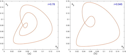3c) where 0<r<1 is a free parameter. 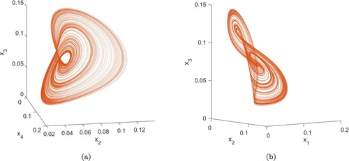We find that chaotic attractor can occur in this Atkinson–Allen model of four species for some big r, i.e., some small survival rate $c_1$ of the species 1. For example, when r = 0.775, a chaotic attractor is detected which is shown in Figure 1. The corresponding Lyapunov exponents are 0.00093, 0, $-0.03085$ and $-0.11667$, which implies a Lyapunov dimension ([6,7]) of 2.03. A detailed investigation is shown below. In our context, a dynamical system that shows exponential sensibility of the time development on the initial conditions is called chaotic; see [6,14].

Figure 1. The chaotic attractor for r = 0.775. (a) projection on the $x_2{x}_3{x}_4$ space; (b) projection on the $x_1{x}_2{x}_3$ space.

The 4D Atkinson–Allen model T with the parameters given by (3(3a) $\begin{array}{rl}c& =(1-r,0.3,0.4,0.1{)}^{\tau },\end{array}$(3a) ) has nine boundary fixed points which is independent of r:

• a trivial fixed point (the origin 0);

• four axial fixed points $q_{\{1\}},q_{\{2\}},q_{\{3\}},q_{\{4\}}$ with $q_{\{i\}}$ lying on positive $x_i$-axis;

• three planar fixed points $v_{\{12\}},v_{\{13\}},v_{\{14\}}$ with $v_{\{ij\}}$ lying on the positive cone of the $x_i{x}_j$ subspace;

• a fixed point $w^{\{1\}}$ on the positive cone of the $x_2{x}_3{x}_4$ subspace,

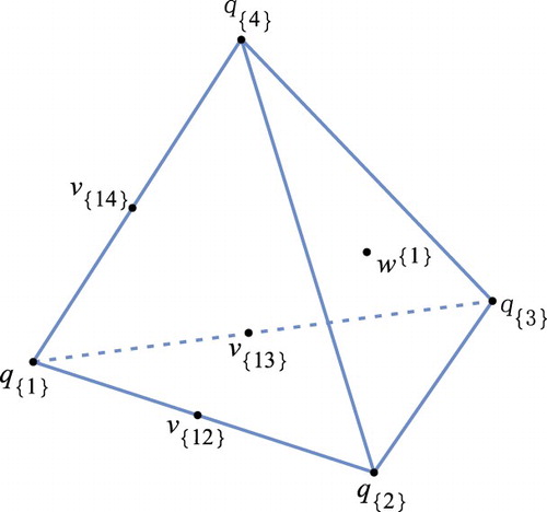
which are all unstable, and a unique positive fixed point p with $p\approx (0.06643,0.05442,0.07562,0.07752{)}^{\tau }.$ Moreover, T admits a 3D carrying simplex Σ homeomorphic to ${\mathrm{\Delta }}^3$; see Figure 2. All the non-trivial boundary fixed points lie on $\mathrm{\partial }\mathrm{\Sigma }$ and p lies in $\dot{\mathrm{\Sigma }}$.

Figure 2. Carrying simplex for the 4D Atkinson–Allen map T with the parameters given by (3(3a) $\begin{array}{rl}c& =(1-r,0.3,0.4,0.1{)}^{\tau },\end{array}$(3a) ). A fixed point on the boundary is represented by a closed dot •.

2.1. Boundary dynamics

Note that each coordinate plane ${\pi }_i$ is positively invariant under T, and $T{|}_{{\pi }_i}$ is a 3D Atkinson–Allen model which admits a 2D carrying simplex, where $T{|}_{{\pi }_i}$ is the restriction of T to ${\pi }_i$. $\mathrm{\partial }\mathrm{\Sigma }$ is composed of the 2D carrying simplices of $T{|}_{{\pi }_i}$, i.e. $\mathrm{\partial }\mathrm{\Sigma }={\cup }_{i=1}^4(\mathrm{\partial }\mathrm{\Sigma }{)}_i$, where $(\mathrm{\partial }\mathrm{\Sigma }{)}_i=\mathrm{\partial }\mathrm{\Sigma }\cap {\pi }_i$ is the carrying simplex of $T{|}_{{\pi }_i}$. Now we study the dynamics of the four 3D Atkinson–Allen maps $T{|}_{{\pi }_i}$, i = 1, 2, 3, 4.

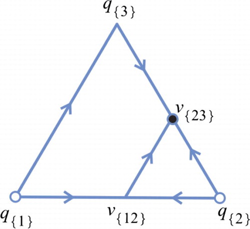
For the general 3D Atkinson–Allen model given by (1(1) $T_i(x)=\frac{(1+s_i)(1-c_i)x_i}{1+\sum _{j=1}^n{b}_{ij}{x}_j}+c_i{x}_i,0<c_i<1,b_{ij},s_i>0,i,j=1,\dots ,n$(1) ), it was shown in [15] that there are a total of 33 stable equivalence classes in terms of simple inequalities on the parameters $b_{ij}$ and $s_i$ by the equivalence relation relative to the boundary dynamics. 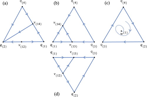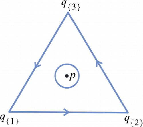According to [15], we know that $T{|}_{{\pi }_4}$ is in class 4 (see Figure 3(d)), $T{|}_{{\pi }_3}$ is in class 8 (see Figure 3(a)), $T{|}_{{\pi }_2}$ is in class 9 (see Figure 3(b)), and $T{|}_{{\pi }_1}$ is in class 27 (see Figure 3(c)) for any 0<r<1, where the sufficient and necessary conditions for classes 4, 8, 9 and 27 are given in the appendix. It then follows that $v_{\{13\}}$ is globally attracting on the interior of ${\pi }_4$ for $T{|}_{{\pi }_4}$, $q_{\{2\}}$ is globally attracting on the interior of ${\pi }_3$ for $T{|}_{{\pi }_3}$, and $v_{\{14\}}$ is globally attracting on the interior of ${\pi }_2$ for $T{|}_{{\pi }_2}$. Therefore, the global dynamics is known for $T{|}_{{\pi }_4}$, $T{|}_{{\pi }_3}$ and $T{|}_{{\pi }_2}$, that is, every non-trivial orbit converges to some boundary fixed point, which is independent of r. Since $T{|}_{{\pi }_1}$ is in class 27, the three edges of $(\mathrm{\partial }\mathrm{\Sigma }{)}_1$ form a heteroclinic cycle and there is a fixed point, i.e. $w^{\{1\}}\approx (0,0.064,0.107,0.059{)}^{\tau }$ in the interior of $(\mathrm{\partial }\mathrm{\Sigma }{)}_1$; see Figure 3(c). The heteroclinic cycle is repelling for $T{|}_{{\pi }_1}$ by Lemma A.5 in the appendix. The Jacobian matrix $DT{|}_{{\pi }_1}(w^{\{1\}})$ has eigenvalues 0.9043, $0.9932\pm 0.0269\mathrm{i}$, which are the three internal eigenvalues of $DT(w^{\{1\}})$. Thus, $w^{\{1\}}$ is stable for $T{|}_{{\pi }_1}$. Note that $T{|}_{{\pi }_1}$ is independent of r, so the boundary dynamics of T is independent of r, and the dynamics on $\mathrm{\partial }\mathrm{\Sigma }$ for T is as shown in Figure 3. On the other hand, the external eigenvalue of $DT(w^{\{1\}})$ is 1 + 0.0208r, so $w^{\{1\}}$ is unstable for T for all 0<r<1.

Figure 3. The phase portrait on $\mathrm{\partial }\mathrm{\Sigma }$ for the 4D Atkinson–Allen map T with the parameters given by (3(3a) $\begin{array}{rl}c& =(1-r,0.3,0.4,0.1{)}^{\tau },\end{array}$(3a) ). (a) the phase portrait on $(\mathrm{\partial }\mathrm{\Sigma }{)}_3$; (b) the phase portrait on $(\mathrm{\partial }\mathrm{\Sigma }{)}_2$; (c) the phase portrait on $(\mathrm{\partial }\mathrm{\Sigma }{)}_1$; (d) the phase portrait on $(\mathrm{\partial }\mathrm{\Sigma }{)}_4$.

2.2. Evolution of the interior attractor

In this subsection, we study the evolution of the attractor within $\dot{\mathrm{\Sigma }}$ for increasing r over the range 0<r<1. The route to chaos was detected as the parameter r is increased. Specifically, in this simple model, we observe that cascades of quasiperiod-doubling bifurcations can lead to chaos. Quasiperiod-doubling bifurcation in our context is referred to the phenomenon that a quasiperiodic curve rounding twice bifurcates from the original one; see Figure 5. We call the bifurcated quasiperiodic curve a 2-quasiperiodic curve. The phenomena, quasiperiod-doubling cascades leading to chaos, have also been observed in [8,33].

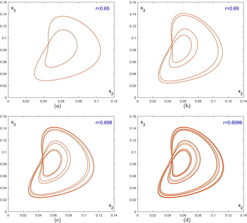
At $r\approx 0.4237$, the positive fixed point p undergoes a supercritical Neimark–Sacker bifurcation with first Lyapunov coefficient $L_1(0)=-0.8747<0$ ([13]). The positive fixed point p is stable for r<0.4237 which can be checked by the Jury test (see [25]). The fixed point p becomes unstable and a stable invariant circle can occur for r>0.4237. Figure 4(b) shows the attracting quasiperiodic curve when r = 0.45. As r is increased from 0.45 the quasiperiodic curve increases in size, until about r = 0.606, where a quasiperiod-doubling cascade begins; that is, the interior attractor evolves from a quasiperiodic curve to a 2-quasiperiodic curve, then to a 4-quasiperiodic curve, then to a 8-quasiperiodic curve, then to a 16-quasiperiodic curve, etc; see Figure 5.

Figure 4. The positive fixed point p undergoes a supercritical Neimark–Sacker bifurcation. (a) a stable fixed point; (b) a stable invariant circle.

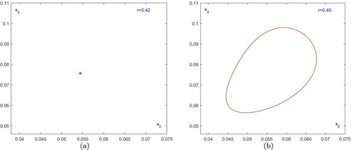
Figure 5. A quasiperiod-doubling cascade begins as r is increased from 0.606. The interior attractor evolves from a quasiperiodic curve to (a) a 2-quasiperiodic curve, then to (b) a 4-quasiperiodic curve, then to (c) a 8-quasiperiodic curve, then to (d) a 16-quasiperiodic curve, and so on.

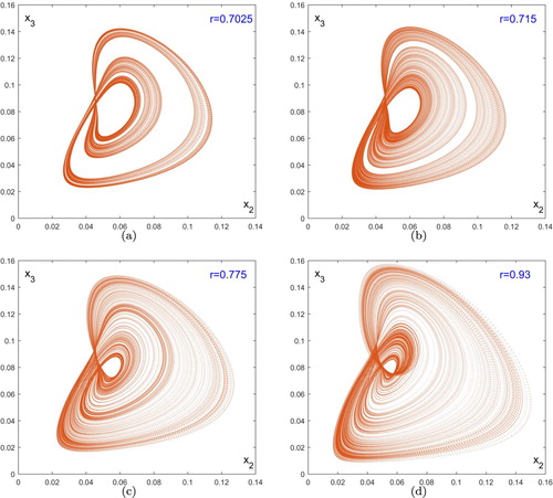
However, such quasiperiod-doubling cascades eventually lead to chaos at about r = 0.7 by noticing that the largest Lyapunov exponent becomes positive for some r>0.7 (see Figure 6). Figure 7(a–d) show the different chaotic attractors for different values of r. Therefore, this example shows a possible route to chaos in the 4D Atkinson–Allen model; that is, cascades of quasiperiod-doubling bifurcations can lead to chaos.

Figure 6. The corresponding largest Lyapunov exponent (the top blue curve) and the second largest Lyapunov exponent (the bottom red curve) as functions of r.

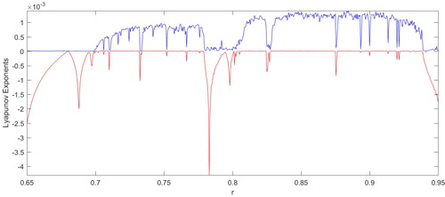
Figure 7. Projection on the $x_2{x}_3$ plane of the chaotic attractors. The successive iterates $T^k$ of T have been applied to the initial point $x_0=(0.01,0.064,0.107,0.059{)}^{\tau }$, producing a sequence asymptotic to the attractor. Here, 2, 00, 000 points of this sequence are plotted, ignoring the first 50, 000 iterates. (a) chaotic attractor for r = 0.7025; (b) chaotic attractor for r = 0.715; (c) chaotic attractor for r = 0.775; (d) chaotic attractor for r = 0.93.

Note that as r is increased, there also exist some quasiperiodic windows, i.e., quasiperiodic curves appear again. As shown in Figure 6, there are some r such that the largest Lyapunov exponent is zero. For example, Figure 8(a) shows that a 3-quasiperiodic curve occurs at r = 0.78. When r>0.939, the chaotic attractor disappears while the attractor becomes an invariant circle. Figure 8(b) shows the attracting invariant circle at r = 0.945.

Figure 8. Projection on the $x_2{x}_3$ plane of the invariant circles. (a) 3-quasiperiodic curve; (b) an invariant circle.

2.3. Invasion caused the system to appear chaotic

Recall that $w^{\{1\}}\approx (0,0.064,0.107,0.059{)}^{\tau }$ is stable for $T{|}_{{\pi }_1}$, that is there is a coexistence of species types 2, 3 and 4, which compete in the rock-scissors-paper manner under Atkinson–Allen dynamics described by $T{|}_{{\pi }_1}$. To begin with, assume the resident populations (species types 2, 3 and 4) are at the steady state $w^{\{1\}}$ and then the mutant (species type 1) is introduced in small quantities. Since the external eigenvalue of $DT(w^{\{1\}})$ is 1 + 0.0208r which is greater than one for all 0<r<1, the species type 1 is able to invade the trimorphic population set by species types 2, 3 and 4 at the steady state $w^{\{1\}}$. Moreover, the invasion can lead to chaos as shown in Figure 7, where the orbit through $x_0=(0.01,0.064,0.107,0.059{)}^{\tau }$ is asymptotic to a chaotic attractor. In other words, when the parameter r is not small (see Figure 6), that is the survival rate of the species type 1 is not large, the invasion by species type 1 into the trimorphic population set by species types 2, 3 and 4 at the steady state $w^{\{1\}}$ caused the system to appear chaotic. For a discussion of these notions and their consequences for evolutionary dynamics we refer the reader to [9–12].

3. Conclusion

Chaos can occur in the four competing species under Atkinson–Allen dynamics described by the invertible map (1(1) $T_i(x)=\frac{(1+s_i)(1-c_i)x_i}{1+\sum _{j=1}^n{b}_{ij}{x}_j}+c_i{x}_i,0<c_i<1,b_{ij},s_i>0,i,j=1,\dots ,n$(1) ) (i.e., n = 4). Varying r, the map undergoes a supercritical Neimark–Sacker bifurcation, which bifurcates a stable quasiperiodic curve, and then the map undergoes a cascade of quasiperiod-doubling bifurcation, and after a critical point becomes chaotic, as illustrated in Figure 5 and Figure 7. Since the map has a 3D carrying simplex, the chaotic attractor is contained in this invariant manifold. This model presents a possible outcome of invasion attempts by an invader (species type 1) into a trimorphic population (species types 2, 3 and 4) competing in the rock-scissors-paper manner; that is, the invasion can lead to chaos. The outcomes of the invasion might be different as the survival rate $c_1$ of the species type 1 varies; that is, the invasion can lead to a coexistence steady state or a quasiperiodic behaviour or a chaotic behaviour which depends on the value of the survival rate $c_1$ of the species type 1. The invasion by species type 1 into the trimorphic population of species types 2, 3 and 4 can lead to a coexistence steady state of the four species when the survival rate $c_1$ of the species type 1 is large while such an invasion can lead to a quasiperiodic behaviour or even a chaotic behaviour when the survival rate $c_1$ of the species type 1 is not large; see Figs. 4–8.

Acknowledgements

The authors are greatly indebted to an anonymous referee for his/her careful and patient reading of our original manuscript, many valuable comments and useful suggestions which led to much improvement in the presentation of our results.

Disclosure statement

No potential conflict of interest was reported by the author(s).

Additional information

Funding

This work is supported by the National Natural Science Foundation of China (NSFC) under grant no. 11771295, Shanghai Gaofeng Project for University Academic Program Development, the Fundamental Research Funds for the Central Universities and the Academy of Finland.

Appendix

Dynamics of the 3D Atkinson–Allen model

In this appendix, we provide the sufficient and necessary conditions with the corresponding phase portraits on the simplices for the classes 4, 8, 9 and 27 of the 3D Atkinson–Allen model (or map) $\hat{T}$ on ${\mathbb{R}}_{+}^3$ given by (A1) ${\hat{T}}_i(x)=\frac{(1+s_i)(1-c_i)x_i}{1+b_{i1}{x}_1+b_{i2}{x}_2+b_{i3}{x}_3}+c_i{x}_i,0<c_i<1,b_{ij},s_i>0,$(A1) i, j = 1, 2, 3. We refer the reader to [15] for the detailed proofs.

The map $\hat{T}$ has three axial fixed points $q_{\{1\}}=(s_1/b_{11},0,0)$, $q_{\{2\}}=(0,s_2/b_{22},0)$ and $q_{\{3\}}=(0,0,s_3/b_{33})$ besides the origin. There may exist a planar fixed point $v_{\{jk\}}$ in the interior of ${\pi }_i$, and there may also exist a positive fixed point p in ${\dot{\mathbb{R}}}_{+}^3$. Let $\hat{\mathrm{\Sigma }}$ be the carrying simplex of the 3D Atkinson–Allen map $\hat{T}$ given by (A1(A1) ${\hat{T}}_i(x)=\frac{(1+s_i)(1-c_i)x_i}{1+b_{i1}{x}_1+b_{i2}{x}_2+b_{i3}{x}_3}+c_i{x}_i,0<c_i<1,b_{ij},s_i>0,$(A1) ). Set ${\gamma }_{ij}=s_j-b_{ji}\frac{s_i}{b_{ii}},{\beta }_{ij}=\frac{s_i{b}_{jj}-s_j{b}_{ij}}{b_{ii}{b}_{jj}-b_{ij}{b}_{ji}}.$

Lemma A.1

The 3D Atkinson–Allen map $\hat{T}$ given by (A1(A1) ${\hat{T}}_i(x)=\frac{(1+s_i)(1-c_i)x_i}{1+b_{i1}{x}_1+b_{i2}{x}_2+b_{i3}{x}_3}+c_i{x}_i,0<c_i<1,b_{ij},s_i>0,$(A1) ) is in the class 4 if and only if there is a permutation σ of the indices $\{1,2,3\},$ after which $\hat{T}$ satisfies the following inequalities

1. ${\gamma }_{12}>0,{\gamma }_{13}<0,{\gamma }_{21}>0,{\gamma }_{23}<0,{\gamma }_{31}>0,{\gamma }_{32}<0;$

2. $b_{12}{\beta }_{23}+b_{13}{\beta }_{32}-r_1<0;$

3. $b_{31}{\beta }_{12}+b_{32}{\beta }_{21}-r_3>0$.

In this case, there are two planar fixed points $v_{\{12\}},v_{\{23\}}$ and there is no positive fixed point. Moreover, $v_{\{12\}}$ is globally attracting on ${\dot{\mathbb{R}}}_{+}^3,$ and the phase portrait on $\hat{\mathrm{\Sigma }}$ is as shown in Figure A1.

Lemma A.2

The 3D Atkinson–Allen map $\hat{T}$ given by (A1(A1) ${\hat{T}}_i(x)=\frac{(1+s_i)(1-c_i)x_i}{1+b_{i1}{x}_1+b_{i2}{x}_2+b_{i3}{x}_3}+c_i{x}_i,0<c_i<1,b_{ij},s_i>0,$(A1) ) is in the class 8 if and only if there is a permutation σ of the indices $\{1,2,3\}$, after which $\hat{T}$ satisfies the following inequalities

1. ${\gamma }_{12}>0,{\gamma }_{13}>0,{\gamma }_{21}>0,{\gamma }_{23}<0,{\gamma }_{31}<0,{\gamma }_{32}<0;$

2. $b_{12}{\beta }_{23}+b_{13}{\beta }_{32}-r_1<0;$

3. $b_{31}{\beta }_{12}+b_{32}{\beta }_{21}-r_3<0$.

In this case, there are two planar fixed points $v_{\{12\}},v_{\{23\}}$ and there is no positive fixed point. Moreover, $q_{\{3\}}$ is globally attracting on ${\dot{\mathbb{R}}}_{+}^3,$ and the phase portrait on $\hat{\mathrm{\Sigma }}$ is as shown in Figure A2.

Figure A1. The phase portrait on $\hat{\mathrm{\Sigma }}$ for the class 4. A fixed point is represented by a closed dot • if it attracts on $\hat{\mathrm{\Sigma }}$, by an open dot ° if it repels on $\hat{\mathrm{\Sigma }}$, and by the intersection of its invariant manifolds if it is a saddle on $\hat{\mathrm{\Sigma }}$.

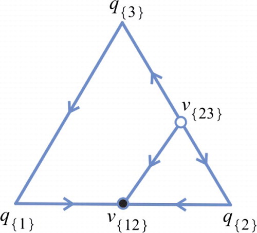
Figure A2. The phase portrait on $\hat{\mathrm{\Sigma }}$ for the class 8. The fixed point notation is as in Figure A1.

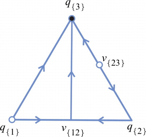
Figure A3. The phase portrait on $\hat{\mathrm{\Sigma }}$ for the class 9. The fixed point notation is as in Figure A1.

Lemma A.3

The 3D Atkinson–Allen map $\hat{T}$ given by (A1(A1) ${\hat{T}}_i(x)=\frac{(1+s_i)(1-c_i)x_i}{1+b_{i1}{x}_1+b_{i2}{x}_2+b_{i3}{x}_3}+c_i{x}_i,0<c_i<1,b_{ij},s_i>0,$(A1) ) is in the class 9 if and only if there is a permutation σ of the indices $\{1,2,3\}$, after which $\hat{T}$ satisfies the following inequalities

1. ${\gamma }_{12}>0,{\gamma }_{13}>0,{\gamma }_{21}>0,{\gamma }_{23}>0,{\gamma }_{31}<0,{\gamma }_{32}>0;$

2. $b_{12}{\beta }_{23}+b_{13}{\beta }_{32}-r_1>0;$

3. $b_{31}{\beta }_{12}+b_{32}{\beta }_{21}-r_3<0$.

In this case, there are two planar fixed points $v_{\{12\}},v_{\{23\}}$ and there is no positive fixed point. Moreover, $v_{\{23\}}$ is globally attracting on ${\dot{\mathbb{R}}}_{+}^3$, and the phase portrait on $\hat{\mathrm{\Sigma }}$ is as shown in Figure A3.

Lemma A.4

The 3D Atkinson–Allen map $\hat{T}$ given by (A1(A1) ${\hat{T}}_i(x)=\frac{(1+s_i)(1-c_i)x_i}{1+b_{i1}{x}_1+b_{i2}{x}_2+b_{i3}{x}_3}+c_i{x}_i,0<c_i<1,b_{ij},s_i>0,$(A1) ) is in the class 27 if and only if there is a permutation σ of the indices $\{1,2,3\},$ after which $\hat{T}$ satisfies the following inequalities ${\gamma }_{12}>0,{\gamma }_{13}<0,{\gamma }_{21}<0,{\gamma }_{23}>0,{\gamma }_{31}>0,{\gamma }_{32}<0.$ In this case, there is a positive fixed point p and $\mathrm{\partial }\hat{\mathrm{\Sigma }}$ is a heteroclinic cycle. The phase portrait on $\hat{\mathrm{\Sigma }}$ is as shown in Figure A4.

Set ${\nu }_{ij}=\frac{(1+s_j)(1-c_j)b_{ii}}{b_{ii}+b_{ji}{s}_i}+c_j$, where $i\ne j$. Let $\vartheta =\ln {\nu }_{12}\ln {\nu }_{23}\ln {\nu }_{31}+\ln {\nu }_{21}\ln {\nu }_{13}\ln {\nu }_{32}.$

Lemma A.5

[15,23]

Assume that the 3D Atkinson–Allen map $\hat{T}$ is in class 27. If $\vartheta <0(\mathrm{resp}.>0),$ then the heteroclinic cycle $\mathrm{\partial }\hat{\mathrm{\Sigma }}$ of $\hat{T}$ is attracting (resp. repelling).

Figure A4. The phase portrait on $\hat{\mathrm{\Sigma }}$ for the class 27. The big circle $◯$ denotes a region of unknown dynamics.

References

- S. Baigent, Geometry of carrying simplices of 3-species competitive Lotka-Volterra systems, Nonlinearity 26 (2013), pp. 1001–1029. doi: 10.1088/0951-7715/26/4/1001
- S. Baigent, and Z. Hou, Global stability of interior and boundary fixed points for Lotka–Volterra systems, Diff. Equation Dyn. Syst. 20 (2012), pp. 53–66. doi: 10.1007/s12591-012-0103-0
- E.C. Balreira, S. Elaydi, and R. Luís, Global stability of higher dimensional monotone maps, J. Diff. Equ. Appl. 23 (2017), pp. 2037–2071. doi: 10.1080/10236198.2017.1388375
- X. Chen, J. Jiang, and L. Niu, On Lotka-Volterra equations with identical minimal intrinsic growth rate, SIAM J. Appl. Dyn. Syst. 14 (2015), pp. 1558–1599. doi: 10.1137/15M1006878
- O. Diekmann, Y. Wang, and P. Yan, Carrying simplices in discrete competitive systems and age-structured semelparous populations, Discrete Contin. Dyn. Syst. 20 (2008), pp. 37–52. doi: 10.3934/dcds.2008.20.37
- J.-P. Eckmann, and D. Ruelle, Ergodic theory of chaos and strange attractors, Rev. Mod. Phys. 57 (1985), pp. 617–656. doi: 10.1103/RevModPhys.57.617
- P. Frederickson, J.L. Kaplan, E.D. Yorke, and J.A. Yorke, The Lyapunov dimension of strange attractors, J. Differ. Equ. 49 (1983), pp. 185–207. doi: 10.1016/0022-0396(83)90011-6
- L. Gardini, R. Lupini, C. Mammana, and M.G. Messia, Bifurcations and transitions to chaos in the three-dimensional Lotka–Volterra map, SIAM J. Appl. Math. 47 (1987), pp. 455–482. doi: 10.1137/0147031
- S.A.H. Geritz, Resident-invader dynamics and the coexistence of similar strategies, J. Math. Biol. 50 (2005), pp. 67–82. doi: 10.1007/s00285-004-0280-8
- S.A.H. Geritz, M. Gyllenberg, F.J.A. Jacobs, and K. Parvinen, Invasion dynamics and attractor inheritance, J. Math. Biol. 44 (2002), pp. 548–560. doi: 10.1007/s002850100136
- S.A.H. Geritz, E. Kisdi, G. Meszéna, and J.A.J. Metz, Evolutionarily singular strategies and the adaptive growth and branching of the evolutionary tree, Evol. Ecol. 12 (1998), pp. 35–57. doi: 10.1023/A:1006554906681
- S.A.H. Geritz, J.A.J. Metz, E. Kisdi, and G. Meszéna, Dynamics of adaptation and evolutionary branching, Phys. Rev. Lett. 78 (1997), pp. 2024–2027. doi: 10.1103/PhysRevLett.78.2024
- W. Govaerts, Y.A. Kuznetsov, H.G.E. Meijer, and N. Neirynck, A study of resonance tongues near a Chenciner bifurcation using MatcontM, in European Nonlinear Dynamics Conference, 24–29, 2011.
- C. Gros, Complex and Adaptive Dynamical Systems A Primer, 3rd ed., Springer-Verlag, Berlin, Heidelberg, 2013.
- M. Gyllenberg, J. Jiang, L. Niu, and P. Yan, On the classification of generalized competitive Atkinson–Allen models via the dynamics on the boundary of the carrying simplex, Discr. Contin. Dyn. Syst. 38 (2018), pp. 615–650. doi: 10.3934/dcds.2018027
- M. Gyllenberg, J. Jiang, and L. Niu, A note on global stability of three-dimensional Ricker models, J. Diff. Equ. Appl. 25 (2019), pp. 142–150. doi: 10.1080/10236198.2019.1566459
- M. Gyllenberg, P. Yan, and Y. Wang, A 3D competitive Lotka–Volterra system with three limit cycles: A falsification of a conjecture by Hofbauer and So, Appl. Math. Lett. 19 (2006), pp. 1–7. doi: 10.1016/j.aml.2005.01.002
- M.W. Hirsch, On existence and uniqueness of the carrying simplex for competitive dynamical systems, J. Biol. Dyn. 2 (2008), pp. 169–179. doi: 10.1080/17513750801939236
- M.W. Hirsch, Systems of differential equations which are competitive or cooperative. III: Competing species, Nonlinearity 1 (1988), pp. 51–71. doi: 10.1088/0951-7715/1/1/003
- J. Jiang and L. Niu, On the equivalent classification of three-dimensional competitive Atkinson/Allen models relative to the boundary fixed points, Discrete Contin. Dyn. Syst. 36 (2016), pp. 217–244.
- J. Jiang and L. Niu, On the equivalent classification of three-dimensional competitive Leslie/Gower models via the boundary dynamics on the carrying simplex, J. Math. Biol. 74 (2017), pp. 1223–1261. doi: 10.1007/s00285-016-1052-y
- J. Jiang and L. Niu, On the validity of Zeeman's classification for three dimensional competitive differential equations with linearly determined nullclines, J. Differ. Eq. 263 (2017), pp. 7753–7781. doi: 10.1016/j.jde.2017.08.022
- J. Jiang, L. Niu, and Y. Wang, On heteroclinic cycles of competitive maps via carrying simplices, J. Math. Biol. 72 (2016), pp. 939–972. doi: 10.1007/s00285-015-0920-1
- Y.A. Kuznetsov, Elements of Applied Bifurcation Theory, Applied Mathematical Sciences, 112, 3rd ed., Springer-Verlag, New York, 2004
- E.R. Lewis, Network Models in Population Biology, Springer-Verlag, Berlin-Heidelberg-New York, 1977.
- Z. Lu and Y. Luo, Three limit cycles for a three-dimensional Lotka–Volterra competitive system with a heteroclinic cycle, Comput. Math. Appl. 46 (2003), pp. 231–238. doi: 10.1016/S0898-1221(03)90027-7
- Ju. I. Neimark, On some cases of periodic motions depending on parameters, Dokl. Akad. Nauk SSSR 129 (1959), pp. 736–739.
- L. Niu and A. Ruiz-Herrera, Trivial dynamics in discrete-time systems: Carrying simplex and translation arcs, Nonlinearity 31 (2018), pp. 2633–2650. doi: 10.1088/1361-6544/aab46e
- L.-I.W. Roeger and L.J.S. Allen, Discrete May-Leonard competition models I, J. Diff. Equ. Appl. 10 (2004), pp. 77–98. doi: 10.1080/10236190310001603662
- A. Ruiz-Herrera, Exclusion and dominance in discrete population models via the carrying simplex, J. Diff. Equ. Appl. 19 (2013), pp. 96–113. doi: 10.1080/10236198.2011.628663
- R. Sacker, On invariant surfaces and bifurcation of periodic solutions of ordinary differential equations, New York University, Rep. IMM-NYU, 333 (1964)
- H.L. Smith, Planar competitive and cooperative difference equations, J. Diff. Equ. Appl. 3 (1998), pp. 335–357. doi: 10.1080/10236199708808108
- L. van Veen, The quasi-periodic doubling cascade in the transition to weak turbulence, Phys. D 210 (2005), pp. 249–261. doi: 10.1016/j.physd.2005.07.020
- P. van den Driessche and M.L. Zeeman, Three-dimensional competitive Lotka–Volterra systems with no periodic orbits, SIAM J. Appl. Math. 58 (1998), pp. 227–234. doi: 10.1137/S0036139997321219
- Y. Wang and J. Jiang, Uniqueness and attractivity of the carrying simplex for discrete-time competitive dynamical systems, J. Differ. Equ. 186 (2002), pp. 611–632. doi: 10.1016/S0022-0396(02)00025-6
- D. Xiao and W. Li, Limit cycles for the competitive three dimensional Lotka-Volterra system, J. Differ. Equ. 164 (2000), pp. 1–15. doi: 10.1006/jdeq.1999.3729
- E.C. Zeeman and M.L. Zeeman, An n-dimensional competitive Lotka-Volterra system is generically determined by the edges of its carrying simplex, Nonlinearity 15 (2002), pp. 2019–2032. doi: 10.1088/0951-7715/15/6/312
- E.C. Zeeman and M.L. Zeeman, From local to global behavior in competitive Lotka-Volterra systems, Trans. Amer. Math. Soc. 355 (2002), pp. 713–734. doi: 10.1090/S0002-9947-02-03103-3
- M.L. Zeeman, Hopf bifurcations in competitive three-dimensional Lotka-Volterra systems, Dyn. Stab. Syst. 8 (1993), pp. 189–216.