Mathematical model for diffusion of the rhizosphere microbial degradation with impulsive feedback control

Abstract

Considering the rhizosphere microbes easily affected by the environmental factors, we formulate a three-dimensional diffusion model of the rhizosphere microbes with the impulsive feedback control to describe the complex degradation and movement by introducing beneficial microbes into the plant rhizosphere. The sufficient conditions for existence of the order-1 periodic solution are obtained by using the geometrical theory of the impulsive semi-dynamical system. We show the impulsive control system tends to an order-1 periodic solution if the control measures are achieved. Furthermore, we investigate the stability of the order-1 periodic solution by means of a novel method introduced in the literature [Y. Ye, The Theory of the Limit Cycle, Shanghai Science and Technology Press, 1984.]. Finally, mathematical results are justified by some numerical simulations.

Keywords:

• Rhizosphere model
• rhizosphere diffusion
• square approximation
• order-1 periodic solution

AMS Subject Classifications:

• 34C05
• 92D25

1. Introduction

It has long been recognized the rhizosphere contains the abundant rhizosphere microbes such as bacteria, fungi, protozoa and nematodes, which can make an important contribution to decomposition of the contaminants [1]. Since the rhizosphere microbe is easily affected by multiple factors including environmental parameters, physiochemical properties of the soil, biological activities of the plants and chemical signals from the plants and bacteria which inhabit the soil adherent to root-system [2], many researchers [3–6] tried to simulate the degradation process by using all kinds of mathematical models. Sung [3] proposed a simple approach to quantify the microbial biomass in the rhizosphere, which was applied to the field microbial biomass data. Kravchenko [4] presented a quantitative model to describe the population of associate nitrogen-fixing in the plant rhizosphere as dependent on the rate of carbon substrate exudation by plant roots. Authors [5] showed the exudation dynamics served as a driving force for microbial and biogeochemical excitation phenomena and led to the development of the emerging attractors and synchronized oscillations of microbial populations and oxygen concentrations. Scott et al. [6] proposed a mathematical model for dispersal of bacterial inoculants colonising the water rhizosphere to describe bacterial growth and movement in the rhizosphere.

In fact, the efficiency of the rhizosphere microbial degradation depends mainly on the concentration of the rhizosphere microbes [7]. The microbial inoculation of the rhizosphere is one of the most promising methods for increasing agricultural productivity and the efficiency of soil pollutant biodegradation [8]. The authors [8] formulated a mathematical modelling of plant growth-promoting rhizobacteria (PGPR) inoculation into the rhizosphere and showed that the competition for limiting resources between the introduced population and the resident microorganisms was the most important factor determining PGPR survival.

Recently, the geometric theory of impulsive semi-dynamical system has been applied into the chemostat model [9–15]. Zhao et al. [13] proposed a nonlinear mathematical model of the rhizosphere microbial degradation with the impulsive feedback control and they investigated sufficient conditions for existence of the order-1 or order-2 periodic solution. Reference [14] investigated a chemostat model with Beddington-DeAnglis uptake function where the sufficient conditions for existence and stability of the order-1 periodic solution were given.

Although the efficiency of the rhizosphere microbial degradation will usually increase before the concentration of the rhizosphere microbes reaches some critical value, the degradation efficiency will decrease if the concentration of the rhizosphere microbes is higher than the critical value(which can be measured in advance). Therefore, it is necessary to reduce the concentration of the rhizosphere microbes lower than the critical value. In this paper, we will construct a three-dimensional diffusion model of differential equations with the impulsive state feedback control by introducing beneficial microbes into the plant rhizosphere so as to further understand the complex dynamics of the rhizosphere microbial degradation.

The paper is organized as follows: a mathematical model of the microbial degradation with impulsive state feedback control is proposed in Section 2. In Section 3, the qualitative analysis of system without impulsive control is given. Furthermore, the existence and stability of order-1 periodic solution are investigated in Section 4. Finally, we give some numerical simulations and a brief discussion.

2. Development of the model and preliminaries

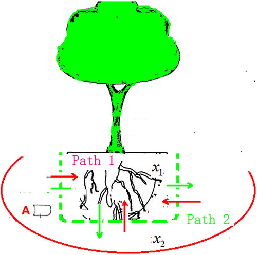
Chemostat is an apparatus for culturing bacterial at a constant rate by controlling the supply of nutrient medium, which is used for representing all kinds of microorganism systems such as lake, waste-water treatment [15–18]. To investigate the dynamics of the process of the rhizosphere microbial degradation, we directly consider the plant rhizosphere system as a chemostat model and divide the rhizosphere system into two patches (defined as patch 1 and patch 2), which is connected by the diffusion of the rhizosphere microbes (see Figure 1).

Figure 1. Illustration of the diffusion and impulsive feedback control. A denotes the monitor which can detect concentration of the indigenous microorganism. Patch 1 shows the region of the inoculation microorganism. Patch 2 denotes the region of the indigenous microorganism.

We introduce the competitive microorganism into the rhizosphere to enhance the degradation efficiency of the indigenous microorganism and prevent the microorganism inhibition. Suppose $S(t)$ is the organic concentration of the rhizosphere and $x_1(t)$ is the concentration of the inoculation microorganism. $x_2(t)$ denotes the concentration of the indigenous microorganism at time t. Based on the references [1–14] and the principle of chemostat model [15–18], the following mathematical model is established: (1) $\{\begin{array}{cc}\begin{array}{c}\frac{\mathrm{d}S}{\mathrm{d}t}=\tilde{Q}(S^0-S)-\frac{{\mu }_{1}S{x}_1}{{\delta }_1}-\frac{{\mu }_{2}S{x}_2}{{\delta }_2},\\ \frac{\mathrm{d}{x}_1}{\mathrm{d}t}=({\mu }_{1}S-\tilde{Q})x_1+\rho (x_2-x_1),\\ \frac{\mathrm{d}{x}_2}{\mathrm{d}t}=({\mu }_{2}S-\tilde{Q})x_2+\rho (x_1-x_2),\end{array}\}& x_2<h,\\ \begin{array}{c}\mathrm{\Delta }{x}_1=\tau ,\\ \mathrm{\Delta }{x}_2=-\theta x_2,\end{array}\}& x_2=h,\end{array}$(1) where all coefficients are positive constants.

The model is derived as follows:

1. When the concentration of the indigenous microorganism reaches the critical value h (predetermined threshold), the negative effects, such as airborne contamination and production inhibition, might occur. To improve the efficiency of the indigenous microorganism and decrease the negative effects, it is necessary to control the concentration of indigenous microorganism lower than the certain level (h) by extracting the indigenous microorganism ($\theta x_2$) and releasing the inoculation microorganism (τ).

2. Suppose $\tilde{Q}$ is the dilution rate, $S^0$ denotes the input concentration of the pollutants. ${\delta }_1$ and ${\delta }_2$ are yield terms(we suppose ${\delta }_1$= ${\delta }_2$=δ for the late convenience of the computation). ${\mu }_1$ and ${\mu }_2$ are the maximum specific growth rates. $\tau >0$ is the amount of the inoculation microorganism and $\theta (0<\theta <1)$ is the ratio of the indigenous microorganism extracted from the rhizosphere. h is a critical value (predetermined threshold). $\mathrm{\Delta }{x}_i=x_i(t^{+})-x_i(t^{-})(i=1,2).$ $\rho (0<\rho <1)$ is diffusive rate between patch 1 and patch 2, which shows the net exchange from patch j to patch i is proportional to the difference $x_j-x_i$(i, j = 1, 2 and $i\ne j$).

Before discussing the periodic solution of system (1(1) $\{\begin{array}{cc}\begin{array}{c}\frac{\mathrm{d}S}{\mathrm{d}t}=\tilde{Q}(S^0-S)-\frac{{\mu }_{1}S{x}_1}{{\delta }_1}-\frac{{\mu }_{2}S{x}_2}{{\delta }_2},\\ \frac{\mathrm{d}{x}_1}{\mathrm{d}t}=({\mu }_{1}S-\tilde{Q})x_1+\rho (x_2-x_1),\\ \frac{\mathrm{d}{x}_2}{\mathrm{d}t}=({\mu }_{2}S-\tilde{Q})x_2+\rho (x_1-x_2),\end{array}\}& x_2<h,\\ \begin{array}{c}\mathrm{\Delta }{x}_1=\tau ,\\ \mathrm{\Delta }{x}_2=-\theta x_2,\end{array}\}& x_2=h,\end{array}$(1) ), we firstly consider the qualitative property of (1(1) $\{\begin{array}{cc}\begin{array}{c}\frac{\mathrm{d}S}{\mathrm{d}t}=\tilde{Q}(S^0-S)-\frac{{\mu }_{1}S{x}_1}{{\delta }_1}-\frac{{\mu }_{2}S{x}_2}{{\delta }_2},\\ \frac{\mathrm{d}{x}_1}{\mathrm{d}t}=({\mu }_{1}S-\tilde{Q})x_1+\rho (x_2-x_1),\\ \frac{\mathrm{d}{x}_2}{\mathrm{d}t}=({\mu }_{2}S-\tilde{Q})x_2+\rho (x_1-x_2),\end{array}\}& x_2<h,\\ \begin{array}{c}\mathrm{\Delta }{x}_1=\tau ,\\ \mathrm{\Delta }{x}_2=-\theta x_2,\end{array}\}& x_2=h,\end{array}$(1) ) without the impulsive effect.

Lemma 2.1

Suppose $\omega (t)=(S(t),x_1(t),x_2(t))$ is a solution of (1(1) $\{\begin{array}{cc}\begin{array}{c}\frac{\mathrm{d}S}{\mathrm{d}t}=\tilde{Q}(S^0-S)-\frac{{\mu }_{1}S{x}_1}{{\delta }_1}-\frac{{\mu }_{2}S{x}_2}{{\delta }_2},\\ \frac{\mathrm{d}{x}_1}{\mathrm{d}t}=({\mu }_{1}S-\tilde{Q})x_1+\rho (x_2-x_1),\\ \frac{\mathrm{d}{x}_2}{\mathrm{d}t}=({\mu }_{2}S-\tilde{Q})x_2+\rho (x_1-x_2),\end{array}\}& x_2<h,\\ \begin{array}{c}\mathrm{\Delta }{x}_1=\tau ,\\ \mathrm{\Delta }{x}_2=-\theta x_2,\end{array}\}& x_2=h,\end{array}$(1) ) subject to $\omega (0^{+})\ge 0,$ then $\omega (t)\ge 0$ for all $t\ge 0,$ and further $\omega (t)>0,t\ge 0$ if $\omega (0^{+})>0.$

From the first three equations, we have $\delta \frac{\mathrm{d}S}{\mathrm{d}t}+\frac{\mathrm{d}{x}_1}{\mathrm{d}t}+\frac{\mathrm{d}{x}_2}{\mathrm{d}t}=\delta \tilde{Q}{S}^0-\tilde{Q}(\delta S+x_1+x_2),$ which shows $\delta S+x_1+x_2=\delta S^0-(\delta S^0-\delta S(0)-x_1(0)-x_2(0)){\mathrm{e}}^{-\tilde{Q}t}$ and we obtain (2) ${\displaystyle \underset{t\to \mathrm{\infty }}{lim}(\delta S+x_1+x_2)=\delta S^0.}$(2) Therefore, we obtain the dynamical behaviour of system (1(1) $\{\begin{array}{cc}\begin{array}{c}\frac{\mathrm{d}S}{\mathrm{d}t}=\tilde{Q}(S^0-S)-\frac{{\mu }_{1}S{x}_1}{{\delta }_1}-\frac{{\mu }_{2}S{x}_2}{{\delta }_2},\\ \frac{\mathrm{d}{x}_1}{\mathrm{d}t}=({\mu }_{1}S-\tilde{Q})x_1+\rho (x_2-x_1),\\ \frac{\mathrm{d}{x}_2}{\mathrm{d}t}=({\mu }_{2}S-\tilde{Q})x_2+\rho (x_1-x_2),\end{array}\}& x_2<h,\\ \begin{array}{c}\mathrm{\Delta }{x}_1=\tau ,\\ \mathrm{\Delta }{x}_2=-\theta x_2,\end{array}\}& x_2=h,\end{array}$(1) ) can be determined by the following system: (3) $\{\begin{array}{cc}\begin{array}{c}\frac{\mathrm{d}{x}_1}{\mathrm{d}t}=({\mu }_1(\delta S^0-x_1-x_2)-\tilde{Q})x_1+\rho (x_2-x_1),\\ \frac{\mathrm{d}{x}_2}{\mathrm{d}t}=({\mu }_2(\delta S^0-x_1-x_2)-\tilde{Q})x_2+\rho (x_1-x_2),\end{array}\}& x_2<h,\\ \begin{array}{c}\mathrm{\Delta }{x}_1=\tau ,\\ \mathrm{\Delta }{x}_2=-\theta x_2,\end{array}\}& x_2=h.\end{array}$(3)

3. Qualitative analysis

Before discussing the periodic solution of system (3(3) $\{\begin{array}{cc}\begin{array}{c}\frac{\mathrm{d}{x}_1}{\mathrm{d}t}=({\mu }_1(\delta S^0-x_1-x_2)-\tilde{Q})x_1+\rho (x_2-x_1),\\ \frac{\mathrm{d}{x}_2}{\mathrm{d}t}=({\mu }_2(\delta S^0-x_1-x_2)-\tilde{Q})x_2+\rho (x_1-x_2),\end{array}\}& x_2<h,\\ \begin{array}{c}\mathrm{\Delta }{x}_1=\tau ,\\ \mathrm{\Delta }{x}_2=-\theta x_2,\end{array}\}& x_2=h.\end{array}$(3) ), we should consider the qualitative properties of (3(3) $\{\begin{array}{cc}\begin{array}{c}\frac{\mathrm{d}{x}_1}{\mathrm{d}t}=({\mu }_1(\delta S^0-x_1-x_2)-\tilde{Q})x_1+\rho (x_2-x_1),\\ \frac{\mathrm{d}{x}_2}{\mathrm{d}t}=({\mu }_2(\delta S^0-x_1-x_2)-\tilde{Q})x_2+\rho (x_1-x_2),\end{array}\}& x_2<h,\\ \begin{array}{c}\mathrm{\Delta }{x}_1=\tau ,\\ \mathrm{\Delta }{x}_2=-\theta x_2,\end{array}\}& x_2=h.\end{array}$(3) ) without the impulsive effect. (4) $\{\begin{array}{l}\frac{\mathrm{d}{x}_1}{\mathrm{d}t}=({\mu }_1(\delta S^0-x_1-x_2)-\tilde{Q})x_1+\rho (x_2-x_1),\\ \frac{\mathrm{d}{x}_2}{\mathrm{d}t}=({\mu }_2(\delta S^0-x_1-x_2)-\tilde{Q})x_2+\rho (x_1-x_2).\end{array}$(4) To obtain the equilibria of the system (4(4) $\{\begin{array}{l}\frac{\mathrm{d}{x}_1}{\mathrm{d}t}=({\mu }_1(\delta S^0-x_1-x_2)-\tilde{Q})x_1+\rho (x_2-x_1),\\ \frac{\mathrm{d}{x}_2}{\mathrm{d}t}=({\mu }_2(\delta S^0-x_1-x_2)-\tilde{Q})x_2+\rho (x_1-x_2).\end{array}$(4) ), we define (5) $\{\begin{array}{l}({\mu }_1(\delta S^0-x_1-x_2)-\tilde{Q})x_1+\rho (x_2-x_1)=0,\\ ({\mu }_2(\delta S^0-x_1-x_2)-\tilde{Q})x_2+\rho (x_1-x_2)=0,\end{array}$(5) we obtain $x_2={\displaystyle (\kappa x_1-\mu x_1^2)/({\mu }_1{x}_1-\rho ),}$ and (6) $\begin{array}{rl}& ({\mu }_1-{\mu }_2)(2\rho +\tilde{Q})x_1^3+({\mu }_1\kappa \xi +{\mu }_1\xi \rho -{\mu }_2{\kappa }^2-2{\mu }_1{\rho }^2+{\mu }_2\kappa \rho )x_1^2\\ & +\rho ({\rho }^2-\kappa \xi )x_1=0,\end{array}$(6) where $\kappa ={\mu }_1\delta S^0-\tilde{Q}-\rho ,\xi ={\mu }_2\delta S^0-\tilde{Q}-\rho$ (Furthermore, $\kappa >0,\xi >0$ according to (2(2) ${\displaystyle \underset{t\to \mathrm{\infty }}{lim}(\delta S+x_1+x_2)=\delta S^0.}$(2) )).

Obviously, Equation (6(6) $\begin{array}{rl}& ({\mu }_1-{\mu }_2)(2\rho +\tilde{Q})x_1^3+({\mu }_1\kappa \xi +{\mu }_1\xi \rho -{\mu }_2{\kappa }^2-2{\mu }_1{\rho }^2+{\mu }_2\kappa \rho )x_1^2\\ & +\rho ({\rho }^2-\kappa \xi )x_1=0,\end{array}$(6) ) has a solution $x_1=0$ and a positive solution $x_1=x_1^{\ast }$ for ${\mu }_1>{\mu }_2$ and ${\rho }^2<\kappa \xi .$ Thus, system (4(4) $\{\begin{array}{l}\frac{\mathrm{d}{x}_1}{\mathrm{d}t}=({\mu }_1(\delta S^0-x_1-x_2)-\tilde{Q})x_1+\rho (x_2-x_1),\\ \frac{\mathrm{d}{x}_2}{\mathrm{d}t}=({\mu }_2(\delta S^0-x_1-x_2)-\tilde{Q})x_2+\rho (x_1-x_2).\end{array}$(4) ) has a trivial equilibria $E_0(0,0)$ and a positive equilibrium $E^{\ast }(x_1^{\ast },x_2^{\ast })$ (${\mu }_1>{\mu }_2$ and ${\rho }^2<\kappa \xi$).

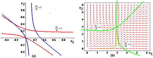
Let the parameters with ${\mu }_1=10,{\mu }_2=6,\delta =0.5,\tilde{Q}=0.55,\rho =0.23,S^0=8,$ we can compute the positive equilibrium $E^{\ast }(0.2119167866,0.1983460985)$[see Figure 2(a)] and Figure 2(b) shows the vector field of system (4(4) $\{\begin{array}{l}\frac{\mathrm{d}{x}_1}{\mathrm{d}t}=({\mu }_1(\delta S^0-x_1-x_2)-\tilde{Q})x_1+\rho (x_2-x_1),\\ \frac{\mathrm{d}{x}_2}{\mathrm{d}t}=({\mu }_2(\delta S^0-x_1-x_2)-\tilde{Q})x_2+\rho (x_1-x_2).\end{array}$(4) ) with the parameters ${\mu }_1=10,{\mu }_2=6,\delta =0.5,\tilde{Q}=0.55,\rho =0.23,S^0=8.$

Figure 2. (a) The intersection point of the two isoclinal lines with the parameters ${\mu }_1=10,{\mu }_2=6,\delta =0.5,\tilde{Q}=0.55,\rho =0.23,S^0=8.$ (b) The vector field of system (3.1) with the parameters ${\mu }_1=10,{\mu }_2=6,\delta =0.6,\tilde{Q}=0.55,\rho =0.23,S^0=8.$

Next, we discuss the local stability of the trivial equilibrium $E_0(0,0)$. The Jacobian matrix evaluated at the point $E_0(0,0)$ is $J(E_0)=\left(\begin{array}{cc}{\mu }_1\delta S^0-\tilde{Q}-\rho & \rho \\ \rho & {\mu }_2\delta S^0-\tilde{Q}-\rho \end{array}\right).$ Defining the eigenvalues of $J(E_0)$ by ${\lambda }_1$ and ${\lambda }_2,$ we have ${\lambda }_1+{\lambda }_2=({\mu }_1+{\mu }_2)\delta S^0-2\tilde{Q}-2\rho$, ${\lambda }_1{\lambda }_2=({\mu }_1\delta S^0-\tilde{Q}-\rho )({\mu }_2\delta S^0-\tilde{Q}-\rho )-{\rho }^2=\kappa \xi -{\rho }^2>0.$ Thus, trivial equilibria $E_0(0,0)$ is unstable node.

Theorem 3.1

The positive equilibrium $(x_1^{\ast },x_2^{\ast })$ is globally asymptotically stable if $\kappa +\xi <2{\mu }_1{x}_1^{\ast }+{\mu }_1{x}_2^{\ast }+2{\mu }_2{x}_2^{\ast }+{\mu }_2{x}_1^{\ast }$ holds, where $\kappa ,\xi$ are given above.

Proof.

Firstly, we analyse the local stability of the positive equilibrium. The Jacobian matrix at $E^{\ast }(x_1^{\ast },x_2^{\ast })$ is given as follows: $\begin{array}{rl}& det\left(\begin{array}{cc}\lambda -({\mu }_1\delta S^0-\tilde{Q}-\rho -2{\mu }_1{x}_1^{\ast }-{\mu }_1{x}_2^{\ast })& -(\rho -{\mu }_1{x}_2^{\ast })\\ -(\rho -{\mu }_2{x}_1^{\ast })& \lambda -({\mu }_2\delta S^0-\tilde{Q}-\rho -2{\mu }_2{x}_2^{\ast }-{\mu }_2{x}_1^{\ast })\end{array}\right)\\ & =0.\end{array}$ We have (7) $\begin{array}{rl}& {\lambda }^2-(\kappa -2{\mu }_1{x}_1^{\ast }-{\mu }_1{x}_2^{\ast }+\xi -2{\mu }_2{x}_2^{\ast }-{\mu }_2{x}_1^{\ast })\lambda +\kappa \xi -{\rho }^2\\ & +{\displaystyle \frac{\rho ({\mu }_1{x_1^{\ast }}^3+{\mu }_2{x_2^{\ast }}^3+{\mu }_1{x}_1^{\ast }{x_2^{\ast }}^2+{\mu }_2{x_1^{\ast }}^2{x}_2^{\ast })}{x_1^{\ast }{x}_2^{\ast }}=0,}\end{array}$(7) where $\kappa ={\mu }_1\delta S^0-\tilde{Q}-\rho ,\xi ={\mu }_2\delta S^0-\tilde{Q}-\rho .$ From (6(6) $\begin{array}{rl}& ({\mu }_1-{\mu }_2)(2\rho +\tilde{Q})x_1^3+({\mu }_1\kappa \xi +{\mu }_1\xi \rho -{\mu }_2{\kappa }^2-2{\mu }_1{\rho }^2+{\mu }_2\kappa \rho )x_1^2\\ & +\rho ({\rho }^2-\kappa \xi )x_1=0,\end{array}$(6) ), we have ${\lambda }_1{\lambda }_2=\kappa \xi -{\rho }^2+{\displaystyle \frac{\rho ({\mu }_1{{x_1}^{\ast }}^3+{\mu }_2{x_2^{\ast }}^3+{\mu }_1{x}_1^{\ast }{x_2^{\ast }}^2+{\mu }_2{x_1^{\ast }}^2{x}_2^{\ast })}{x_1^{\ast }{x}_2^{\ast }}>0}$ while $\kappa \xi >{\rho }^2$ holds. If ${\lambda }_1+{\lambda }_2=\kappa -2{\mu }_1{x}_1^{\ast }-{\mu }_1{x}_2^{\ast }+\xi -2{\mu }_2{x}_2^{\ast }-{\mu }_2{x}_1^{\ast }<0$ is satisfied, then positive equilibrium $E^{\ast }(x_1^{\ast },x_2^{\ast })$ is locally asymptotically stable. That is, the positive equilibrium $E^{\ast }(x_1^{\ast },x_2^{\ast })$ is locally asymptotically stable for $\kappa +\xi <2{\mu }_1{x}_1^{\ast }+{\mu }_1{x}_2^{\ast }+2{\mu }_2{x}_2^{\ast }+{\mu }_2{x}_1^{\ast }$, where $\kappa ,\xi$ are given above.

We consider a Lyapunov function given by $V(x_1,x_2)=c_1(x_1-x_1^{\ast }\ln x_1)+c_2(x_2-x_2^{\ast }\ln x_2),$ where $c_1$ and $c_2$ are positive constant. The derivative of $V(x_1,x_2)$ along the system (4(4) $\{\begin{array}{l}\frac{\mathrm{d}{x}_1}{\mathrm{d}t}=({\mu }_1(\delta S^0-x_1-x_2)-\tilde{Q})x_1+\rho (x_2-x_1),\\ \frac{\mathrm{d}{x}_2}{\mathrm{d}t}=({\mu }_2(\delta S^0-x_1-x_2)-\tilde{Q})x_2+\rho (x_1-x_2).\end{array}$(4) ) is described as follows: $\begin{array}{rl}\frac{\mathrm{d}V}{\mathrm{d}t}& =-(c_1{\mu }_1(x_1-x_1^{\ast }{)}^2+(c_1{\mu }_1+c_2{\mu }_2)(x_1-x_1^{\ast })(x_2-x_2^{\ast })+c_2{\mu }_2(x_2-x_2^{\ast }{)}^2)\\ & -\frac{c_1\rho x_2(x_1-x_1^{\ast }{)}^2}{x_1{x}_1^{\ast }}-\frac{c_2\rho x_1(x_2-x_2^{\ast }{)}^2}{x_2{x}_2^{\ast }}.\end{array}$ We obtain $\mathrm{d}V/\mathrm{d}t\le 0$ by choosing $c_1={\mu }_1/4,c_2={\mu }_2/4$, which implies the positive equilibrium $(x_1^{\ast },x_2^{\ast })$ is globally asymptotically stable.

4. Existence and stability of the order-1 periodic solution

Definition 4.1

[19]

A general planar impulsive semi-dynamical systems with the state-dependent feedback control is presented in the following: (8) $\{\begin{array}{cc}\begin{array}{c}\frac{\mathrm{d}x}{\mathrm{d}t}=P(x,y),\\ \frac{\mathrm{d}y}{\mathrm{d}t}=Q(x,y),\end{array}\}& (x,y)\notin M(x,y),\\ \begin{array}{c}\mathrm{\Delta }x=\alpha (x,y),\\ \mathrm{\Delta }y=\beta (x,y),\end{array}\}& (x,y)\in M(x,y).\end{array}$(8) The solution of system (8(8) $\{\begin{array}{cc}\begin{array}{c}\frac{\mathrm{d}x}{\mathrm{d}t}=P(x,y),\\ \frac{\mathrm{d}y}{\mathrm{d}t}=Q(x,y),\end{array}\}& (x,y)\notin M(x,y),\\ \begin{array}{c}\mathrm{\Delta }x=\alpha (x,y),\\ \mathrm{\Delta }y=\beta (x,y),\end{array}\}& (x,y)\in M(x,y).\end{array}$(8) ) is denoted by $(\mathrm{\Omega },f,\phi ,M)$. Suppose the initial point of mapping $p\in \mathrm{\Omega }=R_{+}^{2}M(x,y)$ is given, ϕ is a continuous mapping $\phi (M)=N$, φ is called as impulse mapping, where $M(x,y)$ and $N(x,y)$ are straight lines or curves on the plane in the positive quadrant $R_{+}^2=\{(x,y)\in R:x\ge 0,y\ge 0\}$. $M(x,y)$ denotes the impulsive set and $N(x,y)$ is the phase set.

Definition 4.2

[19]

Let M denote the impulsive set and N be the phase set. Suppose $g:N\to N$ be a mapping. For any point $P\in N,$ there exists a $t_1>0$ such that $F(P)=f(P,t_1)=P_1\in M,P_1^{+}=\phi (P_1)\in N$, then $g(P)=l(P_1^{+})-l(P)$ is called the successor function of point P and the point $P_1^{+}$ is called the successor point of P.

4.1. Existence of the order-1 periodic solution

In this section, we denote the impulsive set $M=\{(x_1,x_2)\in R_{+}^2|x_1\ge 0,x_2=h\}$, the impulsive function $\phi (x_1,h)=(x_1+\tau ,(1-\theta )x_2)$, and the phase set $N=\{(x_1,x_2)\in R_{+}^2|x_1\ge \tau ,x_2=(1-\theta )h\}.$ From the above analysis, we obtain the positive equilibrium is globally asymptotically stable. In the following, we investigate the existence of the order-1 periodic solution of system (3(3) $\{\begin{array}{cc}\begin{array}{c}\frac{\mathrm{d}{x}_1}{\mathrm{d}t}=({\mu }_1(\delta S^0-x_1-x_2)-\tilde{Q})x_1+\rho (x_2-x_1),\\ \frac{\mathrm{d}{x}_2}{\mathrm{d}t}=({\mu }_2(\delta S^0-x_1-x_2)-\tilde{Q})x_2+\rho (x_1-x_2),\end{array}\}& x_2<h,\\ \begin{array}{c}\mathrm{\Delta }{x}_1=\tau ,\\ \mathrm{\Delta }{x}_2=-\theta x_2,\end{array}\}& x_2=h.\end{array}$(3) ) under this condition.

Obviously, the trajectories starting from the region $x_2>x_2^{\ast }$ will tend to the positive equilibrium $E(x_1^{\ast },x_2^{\ast })$ after impulsive effect of at most one time.

Theorem 4.1

If $x_2<x_2^{\ast },$ then system (3(3) $\{\begin{array}{cc}\begin{array}{c}\frac{\mathrm{d}{x}_1}{\mathrm{d}t}=({\mu }_1(\delta S^0-x_1-x_2)-\tilde{Q})x_1+\rho (x_2-x_1),\\ \frac{\mathrm{d}{x}_2}{\mathrm{d}t}=({\mu }_2(\delta S^0-x_1-x_2)-\tilde{Q})x_2+\rho (x_1-x_2),\end{array}\}& x_2<h,\\ \begin{array}{c}\mathrm{\Delta }{x}_1=\tau ,\\ \mathrm{\Delta }{x}_2=-\theta x_2,\end{array}\}& x_2=h.\end{array}$(3) ) has a unique order-1 periodic solution.

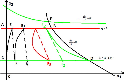
Proof.

Suppose the impulsive set M intersects the $x_2-$axis at the point A and the isoclinal line $\mathrm{d}{x}_1/\mathrm{d}t=0$ at the point B. The phase set N intersects the $x_2-$axis at the point C and the isoclinal line $\mathrm{d}{x}_1/\mathrm{d}t=0$ at the point D. The trajectory starting from the point C intersects the impulsive set M at the point E and reaches the point F due to the impulsive effect $\mathrm{\Delta }{x}_1=\tau ,\mathrm{\Delta }{x}_2=-\theta x_2$. The point F is the successor point of the point C. Thus the successor function of the point C satisfies $f(C)=x_{1F}-x_{1C}>0.$ Similarly, the trajectory from the point D inevitably intersects the line segment AB at the point $E_2.$ The point $E_2$ is mapped into the point $F_2$ after pulses. Furthermore, point $F_2$ is surely on the left of point D from the property of the vector field, hence the successor function of the point D becomes $f(D)=x_{1F}-x_{1D}<0.$ According to the continuity of the successor function, we obtain that there exists a point $F_3$ such that $f(F_3)=0,$ that is, system (3(3) $\{\begin{array}{cc}\begin{array}{c}\frac{\mathrm{d}{x}_1}{\mathrm{d}t}=({\mu }_1(\delta S^0-x_1-x_2)-\tilde{Q})x_1+\rho (x_2-x_1),\\ \frac{\mathrm{d}{x}_2}{\mathrm{d}t}=({\mu }_2(\delta S^0-x_1-x_2)-\tilde{Q})x_2+\rho (x_1-x_2),\end{array}\}& x_2<h,\\ \begin{array}{c}\mathrm{\Delta }{x}_1=\tau ,\\ \mathrm{\Delta }{x}_2=-\theta x_2,\end{array}\}& x_2=h.\end{array}$(3) ) exists an order-1 periodic solution (see Figure 3).

Figure 3. The existence of order-1 periodic solution of system (3(3) $\{\begin{array}{cc}\begin{array}{c}\frac{\mathrm{d}{x}_1}{\mathrm{d}t}=({\mu }_1(\delta S^0-x_1-x_2)-\tilde{Q})x_1+\rho (x_2-x_1),\\ \frac{\mathrm{d}{x}_2}{\mathrm{d}t}=({\mu }_2(\delta S^0-x_1-x_2)-\tilde{Q})x_2+\rho (x_1-x_2),\end{array}\}& x_2<h,\\ \begin{array}{c}\mathrm{\Delta }{x}_1=\tau ,\\ \mathrm{\Delta }{x}_2=-\theta x_2,\end{array}\}& x_2=h.\end{array}$(3) ) for $x_2<x_2^{\ast }.$

4.2. Stability of the order-1 periodic solution

In the following, we will present some Lemmas of the continuous dynamic system [20] to investigate the stability of the order-1 periodic solution.

Lemma 4.2

[20]

Suppose the function $\overline{s}=f(s)$ is a continuous map from the line segment N to itself and s = 0 is a fixed point of the continuous map $f(s).$ The fixed point s = 0 is stable(unstable) if the part near origin of curve $\overline{s}=f(s)$ on the plane $(s,\overline{s})$ lies in the interior of the domain $|{\displaystyle \overline{s}/s|\le 1-\epsilon (\ge 1+\epsilon ),\epsilon >0.}$

Lemma 4.3

[20]

If $\overline{s}=f(s)$ is continuous and derivative at the neighbourhood of the point $s=0,$ the fixed point s = 0 is stable(unstable) for $|{\displaystyle \mathrm{d}\overline{s}/\mathrm{d}s|{|}_{s=0}<1(>1).}$

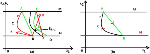
In Figure 4(a), we suppose rectangular coordinate of B is $(\phi (s),\psi (s))$ and obtain the relation of the point $B_k$ between the rectangular coordinates $(x,y)$ and curvilinear coordinates $(s,n)$ by using the geometric method. Thus we have: (9) $x=\phi (s)-n{\psi }^{\prime }(s),y=\psi (s)+n{\phi }^{\prime }(s),$(9) where ${\phi }^{\prime }(s)=\mathrm{d}x/\mathrm{d}s{|}_B=P_0/P_0^2+Q_0^2,\mathrm{d}y/\mathrm{d}s{|}_B=Q_0/P_0^2+Q_0^2.$ $P_0$ and $Q_0$ are the values of P, Q at the point B, that is, $P_0=P(\phi (s),\psi (s)),Q_0=Q(\phi (s),\psi (s)).$

Figure 4. (a) The stability of the order-1 periodic solution of system (3(3) $\{\begin{array}{cc}\begin{array}{c}\frac{\mathrm{d}{x}_1}{\mathrm{d}t}=({\mu }_1(\delta S^0-x_1-x_2)-\tilde{Q})x_1+\rho (x_2-x_1),\\ \frac{\mathrm{d}{x}_2}{\mathrm{d}t}=({\mu }_2(\delta S^0-x_1-x_2)-\tilde{Q})x_2+\rho (x_1-x_2),\end{array}\}& x_2<h,\\ \begin{array}{c}\mathrm{\Delta }{x}_1=\tau ,\\ \mathrm{\Delta }{x}_2=-\theta x_2,\end{array}\}& x_2=h.\end{array}$(3) ) for $x_2<x_2^{\ast }.$ (b) ${\mathrm{\Gamma }}^n$ is the order-1 periodic solution of system (11(11) $\{\begin{array}{cc}\begin{array}{c}\frac{\mathrm{d}{x}_1}{\mathrm{d}t}=({\mu }_1(\delta S^0-x_1-x_2)-\tilde{Q})x_1+\rho (x_2-x_1),\\ \frac{\mathrm{d}{x}_2}{\mathrm{d}t}=({\mu }_2(\delta S^0-x_1-x_2)-\tilde{Q})x_2+\rho (x_1-x_2),\end{array}\}& x_2<h,\\ \begin{array}{c}\mathrm{\Delta }{x}_1=\tau ,\\ \mathrm{\Delta }{x}_2=-\theta x_2,\end{array}\}& x_2=h.\end{array}$(11) ).

From Equation (9(9) $x=\phi (s)-n{\psi }^{\prime }(s),y=\psi (s)+n{\phi }^{\prime }(s),$(9) ), we deduce: ${\displaystyle \frac{\mathrm{d}y}{\mathrm{d}x}=\frac{{\psi }^{\prime }(s)+{\phi }^{\prime }(s)\frac{\mathrm{d}n}{\mathrm{d}s}+n{\phi }^{″}(s)}{{\phi }^{\prime }(s)-{\psi }^{\prime }(s)\frac{\mathrm{d}n}{\mathrm{d}s}-n{\phi }^{″}(s)}=\frac{Q(\phi (s)-n{\psi }^{\prime }(s),\psi (s)+n{\phi }^{\prime }(s))}{P(\phi (s)-n{\psi }^{\prime }(s),\psi (s)+n{\phi }^{\prime }(s))},}$ we obtain (10) $\frac{\mathrm{d}n}{\mathrm{d}s}=\frac{Q{\phi }^{\prime }-P{\psi }^{\prime }-n(P{\phi }^{″}+Q{\psi }^{″})}{P{\phi }^{\prime }+Q{\psi }^{\prime }}=F(s,n).$(10) It is easy to obtain n = 0 is a special solution of system (10(10) $\frac{\mathrm{d}n}{\mathrm{d}s}=\frac{Q{\phi }^{\prime }-P{\psi }^{\prime }-n(P{\phi }^{″}+Q{\psi }^{″})}{P{\phi }^{\prime }+Q{\psi }^{\prime }}=F(s,n).$(10) ). Since function P and Q is continuous and derivative, function $F(s,n)$ also exists continuous partial derivative about the parameter n. Thus, we obtain: $\frac{\mathrm{d}n}{\mathrm{d}s}=F_n^{\prime }(s,n){|}_{n=0}\cdot n+o(n).$ By computing, we have $F_n^{\prime }(s,n){|}_{n=0}=\frac{P_0^2(Q_{0y}-P_0{Q}_0(P_{y0}+Q_{x0}))+Q_0^2{P}_{x0}}{(P_0^2+Q_0^2{)}^{3/2}}=H(s).$ Therefore, Equation (10(10) $\frac{\mathrm{d}n}{\mathrm{d}s}=\frac{Q{\phi }^{\prime }-P{\psi }^{\prime }-n(P{\phi }^{″}+Q{\psi }^{″})}{P{\phi }^{\prime }+Q{\psi }^{\prime }}=F(s,n).$(10) ) becomes $\mathrm{d}n/\mathrm{d}s=H(s)n,$ and we obtain $n(s)=n_0\exp ({\int }_0^{l}H(s^{\prime })\mathrm{d}{s}^{\prime }),n(0)=n_0,$ where l is the length of the curve.

For system (3(3) $\{\begin{array}{cc}\begin{array}{c}\frac{\mathrm{d}{x}_1}{\mathrm{d}t}=({\mu }_1(\delta S^0-x_1-x_2)-\tilde{Q})x_1+\rho (x_2-x_1),\\ \frac{\mathrm{d}{x}_2}{\mathrm{d}t}=({\mu }_2(\delta S^0-x_1-x_2)-\tilde{Q})x_2+\rho (x_1-x_2),\end{array}\}& x_2<h,\\ \begin{array}{c}\mathrm{\Delta }{x}_1=\tau ,\\ \mathrm{\Delta }{x}_2=-\theta x_2,\end{array}\}& x_2=h.\end{array}$(3) ), we try to introduce the method of the square approximation to investigate the stability of the order-1 periodic solution by using theory of the limit cycle.

Suppose the orbit starting from the point B intersects the impulsive set M at point A, then jumps into the point B. The closed orbit composed of the curve $S_{BCA}$ and line segment AB is defined as a closed order-1 periodic limit (denoted as Γ, see Figure 4(a). We draw the normal line n passing through $B\in \mathrm{\Gamma }$ and establish the coordinate system $(s,n)$ on the point B. Choose any point $D\in U(A,\epsilon ),\epsilon >0$ and the trajectory starting from the point D intersects vertically $n-$axis at point $B_k$, then intersects impulsive set M at the point E. The point F is defined as the phase point of the point E due to impulsive effect. The trajectory passing trough point F intersects vertically $n-$axis at point $B_{k+1}$ as time t increases again.

In Figure 4(a), $n_0$ represents the ordinate of $B_k$ and n denotes the ordinate of $B_{k+1}.$ The Poincare map transforms $B_k$ into $B_{k+1}$ and the successor function is expressed as $f(n_0)=n$. If $|n/n_0|<1,$ then curve $S_{B_{k}EF{B}_{K+1}}$ starting from the neighbourhood of point B will tend to the closed order-1 periodic limit ${\mathrm{\Gamma }}_{ABC}$($k\to \mathrm{\infty }$), which shows the closed order-1 periodic limit is stable. Thus we have

Theorem 4.4

Suppose l is the length of the closed orbit Γ of system (3(3) $\{\begin{array}{cc}\begin{array}{c}\frac{\mathrm{d}{x}_1}{\mathrm{d}t}=({\mu }_1(\delta S^0-x_1-x_2)-\tilde{Q})x_1+\rho (x_2-x_1),\\ \frac{\mathrm{d}{x}_2}{\mathrm{d}t}=({\mu }_2(\delta S^0-x_1-x_2)-\tilde{Q})x_2+\rho (x_1-x_2),\end{array}\}& x_2<h,\\ \begin{array}{c}\mathrm{\Delta }{x}_1=\tau ,\\ \mathrm{\Delta }{x}_2=-\theta x_2,\end{array}\}& x_2=h.\end{array}$(3) ) and the closed order-1 periodic limit Γ is stable for ${\int }_0^{l}H(s)\mathrm{d}s<0.$

According to the formula of the arc length $\mathrm{d}s=\sqrt{P_0^2+Q_0^2}\mathrm{d}t,$ we obtain $H(s)={\int }_0^T(P_{x0}+Q_{y0})\mathrm{d}t-{\int }_0^T\frac{1}{2}\mathrm{d}/\mathrm{d}t[\ln (P_0^2+Q_0^2)]\mathrm{d}t,$ where $P_{x0}=\mathrm{\partial }P/\mathrm{\partial }x,P_{y0}=\mathrm{\partial }Q/\mathrm{\partial }y.$

Corollary 4.5

[20]

Suppose the integral along the order-1 periodic solution Γ satisfies $H(s)<0$, then the order-1 periodic solution Γ is stable.

Suppose ${\mathrm{\Gamma }}^{\prime }$ is the $T-$periodic solution of system (4(4) $\{\begin{array}{l}\frac{\mathrm{d}{x}_1}{\mathrm{d}t}=({\mu }_1(\delta S^0-x_1-x_2)-\tilde{Q})x_1+\rho (x_2-x_1),\\ \frac{\mathrm{d}{x}_2}{\mathrm{d}t}=({\mu }_2(\delta S^0-x_1-x_2)-\tilde{Q})x_2+\rho (x_1-x_2).\end{array}$(4) ), we obtain the value of the integral equals to zero along the periodic solution of system (4(4) $\{\begin{array}{l}\frac{\mathrm{d}{x}_1}{\mathrm{d}t}=({\mu }_1(\delta S^0-x_1-x_2)-\tilde{Q})x_1+\rho (x_2-x_1),\\ \frac{\mathrm{d}{x}_2}{\mathrm{d}t}=({\mu }_2(\delta S^0-x_1-x_2)-\tilde{Q})x_2+\rho (x_1-x_2).\end{array}$(4) ), that is, $J_{{\mathrm{\Gamma }}^{\prime }}={\int }_0^T\frac{1}{2}\mathrm{d}/\mathrm{d}t[\ln (P_0^2+Q_0^2)]\mathrm{d}t=0.$

Denote $F(x,y)={\displaystyle \frac{1}{2}\mathrm{d}/\mathrm{d}t[\ln (P_0^2+Q_0^2)].}$ In the following, we will prove the value of integral along the closed order-1 periodic limit Γ has a similar result.

Lemma 4.6

Assume the function $F(x,y)$ is continuous and differentiable, then integral along the closed order-1 periodic limit Γ of system (3(3) $\{\begin{array}{cc}\begin{array}{c}\frac{\mathrm{d}{x}_1}{\mathrm{d}t}=({\mu }_1(\delta S^0-x_1-x_2)-\tilde{Q})x_1+\rho (x_2-x_1),\\ \frac{\mathrm{d}{x}_2}{\mathrm{d}t}=({\mu }_2(\delta S^0-x_1-x_2)-\tilde{Q})x_2+\rho (x_1-x_2),\end{array}\}& x_2<h,\\ \begin{array}{c}\mathrm{\Delta }{x}_1=\tau ,\\ \mathrm{\Delta }{x}_2=-\theta x_2,\end{array}\}& x_2=h.\end{array}$(3) ) satisfies ${\displaystyle {\int }_0^T\mathrm{d}F(x,y)/\mathrm{d}t\mathrm{d}t=0,}$ where T is the period of the closed order-1 periodic limit Γ.

Proof.

Suppose Γ is the closed order-1 periodic limit Γ of system (3(3) $\{\begin{array}{cc}\begin{array}{c}\frac{\mathrm{d}{x}_1}{\mathrm{d}t}=({\mu }_1(\delta S^0-x_1-x_2)-\tilde{Q})x_1+\rho (x_2-x_1),\\ \frac{\mathrm{d}{x}_2}{\mathrm{d}t}=({\mu }_2(\delta S^0-x_1-x_2)-\tilde{Q})x_2+\rho (x_1-x_2),\end{array}\}& x_2<h,\\ \begin{array}{c}\mathrm{\Delta }{x}_1=\tau ,\\ \mathrm{\Delta }{x}_2=-\theta x_2,\end{array}\}& x_2=h.\end{array}$(3) ) and $S_{\widehat{BCA}}$ denotes the curve of system (2(2) ${\displaystyle \underset{t\to \mathrm{\infty }}{lim}(\delta S+x_1+x_2)=\delta S^0.}$(2) ) from the point $B(x_{1B},x_{2B})$ to the point $A(x_{1A},x_{2A}),$ where $S_{\widehat{BCA}}(0)=B$, $S_{\widehat{BCA}}(T)=A$. $S_{AB}$ denotes the line segment $\overline{AB}$. Making a time variable $\tau ={\displaystyle n-1/nt,}$ we transform system (3(3) $\{\begin{array}{cc}\begin{array}{c}\frac{\mathrm{d}{x}_1}{\mathrm{d}t}=({\mu }_1(\delta S^0-x_1-x_2)-\tilde{Q})x_1+\rho (x_2-x_1),\\ \frac{\mathrm{d}{x}_2}{\mathrm{d}t}=({\mu }_2(\delta S^0-x_1-x_2)-\tilde{Q})x_2+\rho (x_1-x_2),\end{array}\}& x_2<h,\\ \begin{array}{c}\mathrm{\Delta }{x}_1=\tau ,\\ \mathrm{\Delta }{x}_2=-\theta x_2,\end{array}\}& x_2=h.\end{array}$(3) ) into the following system (11) $\{\begin{array}{cc}\begin{array}{c}\frac{\mathrm{d}{x}_1}{\mathrm{d}t}=({\mu }_1(\delta S^0-x_1-x_2)-\tilde{Q})x_1+\rho (x_2-x_1),\\ \frac{\mathrm{d}{x}_2}{\mathrm{d}t}=({\mu }_2(\delta S^0-x_1-x_2)-\tilde{Q})x_2+\rho (x_1-x_2),\end{array}\}& x_2<h,\\ \begin{array}{c}\mathrm{\Delta }{x}_1=\tau ,\\ \mathrm{\Delta }{x}_2=-\theta x_2,\end{array}\}& x_2=h.\end{array}$(11) Let ${\mathrm{\Gamma }}^n$ denote the closed order-1 periodic limit of system (11(11) $\{\begin{array}{cc}\begin{array}{c}\frac{\mathrm{d}{x}_1}{\mathrm{d}t}=({\mu }_1(\delta S^0-x_1-x_2)-\tilde{Q})x_1+\rho (x_2-x_1),\\ \frac{\mathrm{d}{x}_2}{\mathrm{d}t}=({\mu }_2(\delta S^0-x_1-x_2)-\tilde{Q})x_2+\rho (x_1-x_2),\end{array}\}& x_2<h,\\ \begin{array}{c}\mathrm{\Delta }{x}_1=\tau ,\\ \mathrm{\Delta }{x}_2=-\theta x_2,\end{array}\}& x_2=h.\end{array}$(11) ). Since system (11(11) $\{\begin{array}{cc}\begin{array}{c}\frac{\mathrm{d}{x}_1}{\mathrm{d}t}=({\mu }_1(\delta S^0-x_1-x_2)-\tilde{Q})x_1+\rho (x_2-x_1),\\ \frac{\mathrm{d}{x}_2}{\mathrm{d}t}=({\mu }_2(\delta S^0-x_1-x_2)-\tilde{Q})x_2+\rho (x_1-x_2),\end{array}\}& x_2<h,\\ \begin{array}{c}\mathrm{\Delta }{x}_1=\tau ,\\ \mathrm{\Delta }{x}_2=-\theta x_2,\end{array}\}& x_2=h.\end{array}$(11) ) is topologically equivalent to system (3(3) $\{\begin{array}{cc}\begin{array}{c}\frac{\mathrm{d}{x}_1}{\mathrm{d}t}=({\mu }_1(\delta S^0-x_1-x_2)-\tilde{Q})x_1+\rho (x_2-x_1),\\ \frac{\mathrm{d}{x}_2}{\mathrm{d}t}=({\mu }_2(\delta S^0-x_1-x_2)-\tilde{Q})x_2+\rho (x_1-x_2),\end{array}\}& x_2<h,\\ \begin{array}{c}\mathrm{\Delta }{x}_1=\tau ,\\ \mathrm{\Delta }{x}_2=-\theta x_2,\end{array}\}& x_2=h.\end{array}$(3) ), the property of the closed order-1 periodic limit ${\mathrm{\Gamma }}^n$ is similar to Γ.

Let ${\overline{S}}_{\widehat{BCA}}$ denote the curve of system (11(11) $\{\begin{array}{cc}\begin{array}{c}\frac{\mathrm{d}{x}_1}{\mathrm{d}t}=({\mu }_1(\delta S^0-x_1-x_2)-\tilde{Q})x_1+\rho (x_2-x_1),\\ \frac{\mathrm{d}{x}_2}{\mathrm{d}t}=({\mu }_2(\delta S^0-x_1-x_2)-\tilde{Q})x_2+\rho (x_1-x_2),\end{array}\}& x_2<h,\\ \begin{array}{c}\mathrm{\Delta }{x}_1=\tau ,\\ \mathrm{\Delta }{x}_2=-\theta x_2,\end{array}\}& x_2=h.\end{array}$(11) ) from the point $B(x_{1B},x_{2B})$ to the point $A(x_{1A},x_{2A}),$ where ${\overline{S}}_{\widehat{BCA}}(0)=B$, ${\overline{S}}_{\widehat{BCA}}(n-1/nT)=A$. ${\overline{S}}_{AB}$ denotes the line segment $\overline{AB}$[see Figure 4(b)]. The line segment AB is satisfied as $x_2=x_{2A}-x_{2B}/x_{1A}-x_{1B}(x_1-x_{1A})+x_{2A},x_{1A}\le x_1\le x_{1B}.$ Obviously, system (11(11) $\{\begin{array}{cc}\begin{array}{c}\frac{\mathrm{d}{x}_1}{\mathrm{d}t}=({\mu }_1(\delta S^0-x_1-x_2)-\tilde{Q})x_1+\rho (x_2-x_1),\\ \frac{\mathrm{d}{x}_2}{\mathrm{d}t}=({\mu }_2(\delta S^0-x_1-x_2)-\tilde{Q})x_2+\rho (x_1-x_2),\end{array}\}& x_2<h,\\ \begin{array}{c}\mathrm{\Delta }{x}_1=\tau ,\\ \mathrm{\Delta }{x}_2=-\theta x_2,\end{array}\}& x_2=h.\end{array}$(11) ) is the square approximation of system (3(3) $\{\begin{array}{cc}\begin{array}{c}\frac{\mathrm{d}{x}_1}{\mathrm{d}t}=({\mu }_1(\delta S^0-x_1-x_2)-\tilde{Q})x_1+\rho (x_2-x_1),\\ \frac{\mathrm{d}{x}_2}{\mathrm{d}t}=({\mu }_2(\delta S^0-x_1-x_2)-\tilde{Q})x_2+\rho (x_1-x_2),\end{array}\}& x_2<h,\\ \begin{array}{c}\mathrm{\Delta }{x}_1=\tau ,\\ \mathrm{\Delta }{x}_2=-\theta x_2,\end{array}\}& x_2=h.\end{array}$(3) ), which implies ${\mathrm{\Gamma }}^n\to \mathrm{\Gamma }$ as $t\to \mathrm{\infty }.$ Thus, we have $\begin{array}{rl}& {\oint }_0^T\frac{\mathrm{d}F(x_1,x_2)}{\mathrm{d}t}\mathrm{d}t\\ & ={\int }_0^{(n-1/n)T}\frac{\mathrm{d}F(x_1,x_2)}{\mathrm{d}t}\mathrm{d}t\\ & =\frac{1}{2}{\int }_{BCA}\frac{\mathrm{d}\ln (P_0^2+Q_0^2)}{\mathrm{d}t}\mathrm{d}t+\frac{1}{2}{\int }_{AB}\frac{\mathrm{d}\ln (P_0^2+Q_0^2)}{\mathrm{d}t}\mathrm{d}t\to 0,n\to \mathrm{\infty },\end{array}$ which shows ${\int }_0^T\mathrm{d}F(x_1,x_2)/\mathrm{d}t\mathrm{d}t=0.$

Therefore, we have the following result.

Theorem 4.7

Assume the integral along the order-1 periodic solution Γ of system (3(3) $\{\begin{array}{cc}\begin{array}{c}\frac{\mathrm{d}{x}_1}{\mathrm{d}t}=({\mu }_1(\delta S^0-x_1-x_2)-\tilde{Q})x_1+\rho (x_2-x_1),\\ \frac{\mathrm{d}{x}_2}{\mathrm{d}t}=({\mu }_2(\delta S^0-x_1-x_2)-\tilde{Q})x_2+\rho (x_1-x_2),\end{array}\}& x_2<h,\\ \begin{array}{c}\mathrm{\Delta }{x}_1=\tau ,\\ \mathrm{\Delta }{x}_2=-\theta x_2,\end{array}\}& x_2=h.\end{array}$(3) ) satisfies (12) ${\int }_0^T(\frac{\mathrm{\partial }P}{\mathrm{\partial }x}+\frac{\mathrm{\partial }Q}{\mathrm{\partial }y})\mathrm{d}t<0,$(12) then order-1 periodic solution Γ is stable.

Theorem 4.8

The order-1 periodic solution of system (3(3) $\{\begin{array}{cc}\begin{array}{c}\frac{\mathrm{d}{x}_1}{\mathrm{d}t}=({\mu }_1(\delta S^0-x_1-x_2)-\tilde{Q})x_1+\rho (x_2-x_1),\\ \frac{\mathrm{d}{x}_2}{\mathrm{d}t}=({\mu }_2(\delta S^0-x_1-x_2)-\tilde{Q})x_2+\rho (x_1-x_2),\end{array}\}& x_2<h,\\ \begin{array}{c}\mathrm{\Delta }{x}_1=\tau ,\\ \mathrm{\Delta }{x}_2=-\theta x_2,\end{array}\}& x_2=h.\end{array}$(3) ) is stable.

Proof.

From the first two equations, we have (13) $\frac{\mathrm{\partial }P}{\mathrm{\partial }{x}_1}+\frac{\mathrm{\partial }Q}{\mathrm{\partial }{x}_2}={\mu }_1\delta S^0-\tilde{Q}-\rho -2{\mu }_1{x}_1-{\mu }_1{x}_2+{\mu }_2\delta S^0-\tilde{Q}-\rho -2{\mu }_2{x}_2-{\mu }_2{x}_1.$(13) Since it is difficult to judge the positive or negative of the sign of the expression (13(13) $\frac{\mathrm{\partial }P}{\mathrm{\partial }{x}_1}+\frac{\mathrm{\partial }Q}{\mathrm{\partial }{x}_2}={\mu }_1\delta S^0-\tilde{Q}-\rho -2{\mu }_1{x}_1-{\mu }_1{x}_2+{\mu }_2\delta S^0-\tilde{Q}-\rho -2{\mu }_2{x}_2-{\mu }_2{x}_1.$(13) ), we make a topological transformation $u(x_1,x_2)={\displaystyle 1/x_1{x}_2}$ by using the Dulac's Theorem [20], system (3(3) $\{\begin{array}{cc}\begin{array}{c}\frac{\mathrm{d}{x}_1}{\mathrm{d}t}=({\mu }_1(\delta S^0-x_1-x_2)-\tilde{Q})x_1+\rho (x_2-x_1),\\ \frac{\mathrm{d}{x}_2}{\mathrm{d}t}=({\mu }_2(\delta S^0-x_1-x_2)-\tilde{Q})x_2+\rho (x_1-x_2),\end{array}\}& x_2<h,\\ \begin{array}{c}\mathrm{\Delta }{x}_1=\tau ,\\ \mathrm{\Delta }{x}_2=-\theta x_2,\end{array}\}& x_2=h.\end{array}$(3) ) is topologically equivalent to the following system: $\{\begin{array}{l}{\displaystyle \frac{\mathrm{d}{x}_1}{\mathrm{d}t}=\frac{{\mu }_1\delta S^0-\tilde{Q}-\rho }{x_2}-\frac{{\mu }_1{x}_1}{x_2}-{\mu }_1+\frac{\rho }{x_2}=P(x_1,x_2)u(x_1,x_2)=P_1(x_1,x_2),}\\ {\displaystyle \frac{\mathrm{d}{x}_2}{\mathrm{d}t}=\frac{{\mu }_2\delta S^0-\tilde{Q}-\rho }{x_1}-\frac{{\mu }_2{x}_2}{x_1}-{\mu }_2+\frac{\rho }{x_1}=Q(x_1,x_2)u(x_1,x_2)=Q_1(x_1,x_2),}\end{array}$ we obtain the inequality $\mathrm{\partial }{P}_1/\mathrm{\partial }{x}_1+\mathrm{\partial }{Q}_1/\mathrm{\partial }{x}_2=-({\mu }_1/x_2+{\mu }_2/x_1)<0$ holds for $x_1>0$ and $x_2>0.$ According to Theorem 4.6, we obtain the order-1 periodic solution is stable.

5. Discussion

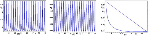
In this paper, we formulate a three-dimensional diffusion model of the rhizosphere microbes with the impulsive feedback control to understand the complex process of the degradation and improve the degradation efficiency. Firstly, the positive equilibrium $E^{\ast }(2.482108142,1.453359144)$ exists by using numerical simulation with the parameters ${\mu }_1=10,{\mu }_2=6,\delta =0.5,\tilde{Q}=0.55,\rho =0.23,S^0=8.$ Globally asymptotical stability of the positive equilibrium $E(x_1^{\ast },x_2^{\ast })$ is proved by methods of Lyapunov function, which means that pollutant concentration $S(t)$, inoculation concentration $x_1(t)$ and indigenous concentration $x_2(t)$ will become saturated and degradation ability has no further improvement. To enhance the degradation efficiency of the rhizosphere microbes, the model of the microbial degradation is proposed based on the impulsive semi-dynamical system. By using the geometric theory of the impulsive semi-dynamical system, we obtain system (3(3) $\{\begin{array}{cc}\begin{array}{c}\frac{\mathrm{d}{x}_1}{\mathrm{d}t}=({\mu }_1(\delta S^0-x_1-x_2)-\tilde{Q})x_1+\rho (x_2-x_1),\\ \frac{\mathrm{d}{x}_2}{\mathrm{d}t}=({\mu }_2(\delta S^0-x_1-x_2)-\tilde{Q})x_2+\rho (x_1-x_2),\end{array}\}& x_2<h,\\ \begin{array}{c}\mathrm{\Delta }{x}_1=\tau ,\\ \mathrm{\Delta }{x}_2=-\theta x_2,\end{array}\}& x_2=h.\end{array}$(3) ) exists an order-1 periodic solution for $h<x_2^{\ast }$, and the simulation is given in Figure 5 with the parameters ${\mu }_1=10,{\mu }_2=6,\delta =0.5,\tilde{Q}=0.55,\rho =0.23,S^0=8,h=0.33<x_2^{\ast }=1.453359144,\tau =2,\theta =\mathrm{0.2.}$ Finally, we investigate the stability of the order-1 periodic solution in terms of the theory of the limit cycle.

Figure 5. Time series and phase portrait of the order-1 periodic solution of system (3(3) $\{\begin{array}{cc}\begin{array}{c}\frac{\mathrm{d}{x}_1}{\mathrm{d}t}=({\mu }_1(\delta S^0-x_1-x_2)-\tilde{Q})x_1+\rho (x_2-x_1),\\ \frac{\mathrm{d}{x}_2}{\mathrm{d}t}=({\mu }_2(\delta S^0-x_1-x_2)-\tilde{Q})x_2+\rho (x_1-x_2),\end{array}\}& x_2<h,\\ \begin{array}{c}\mathrm{\Delta }{x}_1=\tau ,\\ \mathrm{\Delta }{x}_2=-\theta x_2,\end{array}\}& x_2=h.\end{array}$(3) ) with the parameters ${\mu }_1=10,{\mu }_2=6,\delta =0.5,\tilde{Q}=0.55,\rho =0.23,S^0=8,h=0.33,\tau =2,\theta =\mathrm{0.2.}$

Disclosure statement

No potential conflict of interest was reported by the author(s).

Additional information

Funding

This work is supported by Tianzhong scholars programme in Huanghuai University and the project of the Distinguished Professor of colleges and Universities in Henan province.

References

- Z.M. Solaiman and H.M. Anawar, Rhizosphere Microbes Interactions in Medicinal Plants, Springer, 2015.
- S. Haldar and S. Sengupta, Plant-microbe cross-talk in the rhizosphere: insight and biotechnological potential, Open Microbiol. J. 9 (2015), pp. 1–7. doi: 10.2174/1874285801509010001
- K. Sung, J. Kim, C.L. Munster, M.Y. Corapcioglu, S. Park, M.C. Drew, and Y.Y. Chang, A simple approach to modeling microbial biomass in the rhizosphere, Ecol. Modell. 190 (2006), pp. 277–286. doi: 10.1016/j.ecolmodel.2005.04.020
- L.V. Kravchenko, N.S. Strigul, and I.A. Shvytov, Mathematical simulation of the dynamics of interacting populations of rhizosphere microorganisms, Microbiology 73(2) (2004), pp. 189–195. doi: 10.1023/B:MICI.0000023988.11064.43
- B. Faybishenko and F. Molz, Nonlinear rhizosphere dynamics yields synchronized oscillation of microbial population, carbon and oxygen concentration induced by root exudation, Procedia Environ. Sci. 19 (2013), pp. 369–378. doi: 10.1016/j.proenv.2013.06.042
- E.M. Scott, E.A.S. Rattray, J.I. Prosser, K. Killham, L.A. Glover, J.M. Lynch, and M.J. Bazin, Amathematical model for dispersal of bacterial inoculants colonizing the wheat rhizosphere, Soil Biol. Biochem. 27(10) (1995), pp. 1307–1318. doi: 10.1016/0038-0717(95)00050-O
- H.P. Bai, T.L. Weir, L.G. Perry, S. Gilroy, and J.M. Vivanco, The role of root exudates in rhizosphere interaction with plants and other organisms, Annu. Rev. Plant Biol. 57 (2006), pp. 233–266. doi: 10.1146/annurev.arplant.57.032905.105159
- N.S. Strigul and L.V. Kravchenko, Mathematical modeling of PGPR inoculation into the rhizosphere, Environ. Modell. Software 21 (2006), pp. 1158–1171. doi: 10.1016/j.envsoft.2005.06.003
- S. Chen, W. Xu, L. Chen, and Z. Huang, A White-headed langurs impulsive state feedback control model with sparse effect and continuous delay, Commun. Nonlinear Sci. Numer. Simul. 50 (2017), pp. 88–102. doi: 10.1016/j.cnsns.2017.02.003
- Z. Zhao, T. Wang, and L. Chen, Dynamic analysis of a turbidostat model with the feedback control original, Commun. Nonlinear Sci. Numer. Simul. 15 (2010), pp. 1028–1035. doi: 10.1016/j.cnsns.2009.05.016
- K. Sun, A. Kasperski, Y. Tian, and L. Chen, Modelling of the corynebacterium glutamicum biosynthesis under aerobic fermentation conditions, Chem. Eng. Sci. 66 (2011), pp. 4101–4110. doi: 10.1016/j.ces.2011.05.041
- K. Sun, Y. Tian, L. Chen, and A. Kasperski, Nonlinear modeling of a synchronized chemostat with impulsive state feedback control, Math. Comput. Modell. 52 (2010), pp. 227–240. doi: 10.1016/j.mcm.2010.02.012
- Z. Zhao, L. Pang, Z. Zhao, and C. Luo, Impulsive state feedback control of the rhizosphere microbial degradation in the wetland plant, Discrete Dyn. Nat. Soc. 2015 (2015), pp. 612354.
- Z. Li, T. Wang, and L. Chen, Periodic solution of a chemostat model with Beddington-DeAnglis uptake function and impulsive state feedback control, J. Theor. Biol. 261 (2009), pp. 23–32. doi: 10.1016/j.jtbi.2009.07.016
- Z. Zhao, L. Yang, and L. Chen, Impulsive state feedback control of the microorganism culture in a turbidostat, J. Math. Chem. 47 (2010), pp. 1224–1239. doi: 10.1007/s10910-009-9644-z
- M. Chi and W. Zhao, Dynamical analysis of multi-nutrient and single microorganism chemostat model in a polluted environment, Adv. Differ. Equ. 2018 (2018), pp. 120–136. doi: 10.1186/s13662-018-1573-3
- T. Zhang, W. Ma, and X. Meng, Global dynamics of a delayed chemostat model with harvest by impulsive flocculant input, Adv. Differ. Equ. 2017 (2017), pp. 115–132. doi: 10.1186/s13662-017-1163-9
- J. Cao, J. Bao, and P. Wang, Global analysis of a delayed Monod type chemostat model with impulsive input on two substrates, Adv. Differ. Equ. 2015 (2015), pp. 310–322. doi: 10.1186/s13662-015-0623-3
- G. Pang, L. Chen, W. Xu, and G. Fu, A stage structure pest management model with impulsive state feedback control, Commun. Nonlinear Sci. Numer. Simul. 23 (2015), pp. 78–88. doi: 10.1016/j.cnsns.2014.10.033
- Y. Ye, The Theory of the Limit Cycle, Shanghai Science and Technology Press, 1984.