Global convergence dynamics of almost periodic delay Nicholson's blowflies systems

Abstract

We take into account nonlinear density-dependent mortality term and patch structure to deal with the global convergence dynamics of almost periodic delay Nicholson's blowflies system in this paper. To begin with, we prove that the solutions of the addressed system exist globally and are bounded above. What's more, by the methods of Lyapunov function and analytical techniques, we establish new criteria to check the existence and global attractivity of the positive asymptotically almost periodic solution. In the end, we arrange an example to illustrate the effectiveness and feasibility of the obtained results.

Keywords:

• Nicholson's blowflies system
• patch structure
• density-dependent mortality term
• almost periodic solution
• global attractivity

AMS(2000) Subject Classifications:

• 34C25
• 34K13

1. Introduction

There has been a growing concern that the dynamic model plays an important role in many fields including biology system, financial and economic network, physics, and engineering technology [1,11,13,15,16,22,41]. In order to describe the oscillatory fluctuations of the laboratory population of the Australian sheep blowfly Lucilia cuprina, Gurney et al. [7] proposed the following delay Nicholson's blowflies equation: (1) $\frac{\mathrm{d}N(t)}{\mathrm{d}t}=-\delta N(t)+PN(t-T_D){\mathrm{e}}^{-(N(t-T_D)/N_D)}.$(1) Biologically, $N(t)$ represents the size of sexually mature adults at time t, the per capita adult death rate with density-independent value equals δ, $T_D$ is the generation time from eggs to sexually mature adults, and P denotes the maximum possible per capita daily egg production rate. The birth function gets the maximum reproduction value with $N=\frac{1}{N_D}$. The delay Nicholson's blowflies equation offers a suitable benchmark for describing a ‘humped’ relationship between future recruitment and current population as it presents abundant dynamics characteristics, such as global attractivity, complex oscillations and even chaotic behaviour [2,9,10,14,21,23,25,29,31,36,39,42].

In biological system, the stability and instability of population-dynamics process are essentially influenced by the interaction of trophodynamic interactions among individuals [26]. Considering that the lethal fighting or cannibalism is usually inevitable, it is more reasonable to introduce a nonlinear (density-dependent) mortality term to the population model [28]. In addition, some cases of patchiness caused by diffusion instability occur in natural populations [27]. Naturally, by introducing nonlinear density-dependent mortality term and patch structure, the following revised Nicholson's blowflies systems with the Rickers type birth function and the harvesting strategy Type II (cyrtoid) (2) $\begin{array}{rl}{x}_i^{\prime }(t)& =-\frac{a_{ii}(t)x_i(t)}{b_{ii}(t)+x_i(t)}+\sum _{j=1,j\ne i}^n\frac{a_{ij}(t)x_j(t)}{b_{ij}(t)+x_j(t)}\\ & +\sum _{j=1}^m{\beta }_{ij}(t)x_i(t-{\tau }_{ij}(t)){\mathrm{e}}^{-{\gamma }_{ij}(t)x_i(t-{\tau }_{ij}(t))},\end{array}$(2) were proposed in the pioneering works [3,19,34], where $i\in Q=\{1,2,\dots ,n\}$, in ith patch, $(a_{ii}(t)x_i(t))/(b_{ii}(t)+x_i(t))$ is the death rate; ${\beta }_{ij}(t)x_i(t-{\tau }_{ij}(t)){\mathrm{e}}^{-{\gamma }_{ij}(t)x_i(t-{\tau }_{ij}(t))}$ is the birth function involving maturation delays ${\tau }_{ij}(t)$ and gets the maximum reproduce value with $x_i(t-{\tau }_{ij}(t))=(1/{\gamma }_{ij}(t))$; for $i,j\in Q$ and $j\ne i$, $(a_{ij}(t)x_j(t)/(b_{ij}(t)+x_j(t)))$ denotes cooperative connection weight of the populations ith patch and jth patch. Please refer to [5,17,35].

The periodic phenomenon in population dynamics has become a hot topic in recent years, yet there is almost no phenomenon that is purely periodic, and the almost periodic phenomenon is obviously more common [4,18,24]. Consequently, the almost periodic problems for delay Nicholson's blowflies equation and its variants have been intensively investigated in [12,33,37,40]. In particular, if there exists a positive constant $M>\kappa$ such that the following conditions hold: (3) $\begin{array}{rl}& {\gamma }_{ij}(t)M\le \tilde{\kappa },\text{for all }t\in \mathbb{R},i\in Q,j\in I=\{1,2,\dots ,m\},\end{array}$(3) (4) $\begin{array}{rl}& \underset{t\in \mathbb{R}}{sup}\{-\frac{a_{ii}(t)M}{b_{ii}(t)+M}+\sum _{j=1,j\ne i}^n{a}_{ij}(t)+\sum _{j=1}^m\frac{{\beta }_{ij}(t)}{{\gamma }_{ij}(t)}\frac{1}{e}\}<0,i\in Q,\end{array}$(4) (5) $\begin{array}{rl}& \underset{t\in \mathbb{R},s\in [0,\kappa ]}{inf}\{-\frac{a_{ii}(t)}{b_{ii}(t)+s}+\sum _{j=1,j\ne i}^n\frac{a_{ij}(t)}{b_{ij}(t)+M}+\sum _{j=1}^m\frac{{\beta }_{ij}(t)}{{\gamma }_{ij}(t)}{\mathrm{e}}^{-s}\}>0,i\in Q,\end{array}$(5) (6) $\begin{array}{rl}& \underset{t\in \mathbb{R}}{sup}\{-\frac{a_{ii}(t)b_{ii}(t)}{(b_{ii}(t)+M{)}^2}+\sum _{j=1,j\ne i}^n\frac{a_{ij}(t)b_{ij}(t)}{(b_{ij}(t)+\kappa {)}^2}+\frac{1}{{\mathrm{e}}^2}\sum _{j=1}^m{\beta }_{ij}(t)\}<0,i\in Q,\end{array}$(6) where (7) $\begin{array}{r}\begin{array}{rl}& \kappa \in (0,1),{\displaystyle \frac{1-\kappa }{{\mathrm{e}}^{\kappa }}}={\displaystyle \frac{1}{{\mathrm{e}}^2}},\tilde{\kappa }\in (1,+\mathrm{\infty }),\\ & \kappa {\mathrm{e}}^{-\kappa }=\tilde{\kappa }{\mathrm{e}}^{-\tilde{\kappa }},\kappa \approx 0.7215,\tilde{\kappa }\approx 1.3423,\end{array}\end{array}$(7) the authors in [20] built the existence and global stability of almost periodic solutions for system (2(2) $\begin{array}{rl}{x}_i^{\prime }(t)& =-\frac{a_{ii}(t)x_i(t)}{b_{ii}(t)+x_i(t)}+\sum _{j=1,j\ne i}^n\frac{a_{ij}(t)x_j(t)}{b_{ij}(t)+x_j(t)}\\ & +\sum _{j=1}^m{\beta }_{ij}(t)x_i(t-{\tau }_{ij}(t)){\mathrm{e}}^{-{\gamma }_{ij}(t)x_i(t-{\tau }_{ij}(t))},\end{array}$(2) ). Unfortunately, conditions (4(4) $\begin{array}{rl}& \underset{t\in \mathbb{R}}{sup}\{-\frac{a_{ii}(t)M}{b_{ii}(t)+M}+\sum _{j=1,j\ne i}^n{a}_{ij}(t)+\sum _{j=1}^m\frac{{\beta }_{ij}(t)}{{\gamma }_{ij}(t)}\frac{1}{e}\}<0,i\in Q,\end{array}$(4) )–(6(6) $\begin{array}{rl}& \underset{t\in \mathbb{R}}{sup}\{-\frac{a_{ii}(t)b_{ii}(t)}{(b_{ii}(t)+M{)}^2}+\sum _{j=1,j\ne i}^n\frac{a_{ij}(t)b_{ij}(t)}{(b_{ij}(t)+\kappa {)}^2}+\frac{1}{{\mathrm{e}}^2}\sum _{j=1}^m{\beta }_{ij}(t)\}<0,i\in Q,\end{array}$(6) ) have considerable limitations and are not consistent with the actual biological significance. Just as shown in [33,40], for a better biological interpretation, it may be a good choice to replace (4(4) $\begin{array}{rl}& \underset{t\in \mathbb{R}}{sup}\{-\frac{a_{ii}(t)M}{b_{ii}(t)+M}+\sum _{j=1,j\ne i}^n{a}_{ij}(t)+\sum _{j=1}^m\frac{{\beta }_{ij}(t)}{{\gamma }_{ij}(t)}\frac{1}{e}\}<0,i\in Q,\end{array}$(4) )–(6(6) $\begin{array}{rl}& \underset{t\in \mathbb{R}}{sup}\{-\frac{a_{ii}(t)b_{ii}(t)}{(b_{ii}(t)+M{)}^2}+\sum _{j=1,j\ne i}^n\frac{a_{ij}(t)b_{ij}(t)}{(b_{ij}(t)+\kappa {)}^2}+\frac{1}{{\mathrm{e}}^2}\sum _{j=1}^m{\beta }_{ij}(t)\}<0,i\in Q,\end{array}$(6) ) with the following relaxed conditions: (8) $\begin{array}{rl}& M\underset{t\to +\mathrm{\infty }}{lim sup}{\gamma }_{ij}(t)\le \tilde{\kappa },\text{for all }i\in Q,j\in I,\end{array}$(8) (9) $\begin{array}{rl}& \underset{t\in [t_0,+\mathrm{\infty })}{sup}\{-\frac{a_{ii}(t)M}{b_{ii}(t)+M}+\sum _{j=1,j\ne i}^n{a}_{ij}(t)+\sum _{j=1}^m\frac{{\beta }_{ij}(t)}{{\gamma }_{ij}(t)}\frac{1}{e}\}<0,i\in Q,\end{array}$(9) (10) $\begin{array}{rl}& \underset{s\in [0,\kappa ]}{inf}\underset{t\to +\mathrm{\infty }}{lim inf}\{-\frac{a_{ii}(t)}{b_{ii}(t)+s}+\sum _{j=1,j\ne i}^n\frac{a_{ij}(t)}{b_{ij}(t)+M}+\sum _{j=1}^m\frac{{\beta }_{ij}(t)}{{\gamma }_{ij}(t)}{\mathrm{e}}^{-s}\}>0,i\in Q,\end{array}$(10) (11) $\begin{array}{rl}& \underset{t\to +\mathrm{\infty }}{lim sup}\{-\frac{a_{ii}(t)b_{ii}(t)}{(b_{ii}(t)+M{)}^2}+\sum _{j=1,j\ne i}^n\frac{a_{ij}(t)b_{ij}(t)}{(b_{ij}(t)+\kappa {)}^2}+\frac{1}{{\mathrm{e}}^2}\sum _{j=1}^m{\beta }_{ij}(t)\}<0,i\in Q.\end{array}$(11) It is a great pity that (12) $0<l_i\underset{t\in \mathbb{R},s\in [0,\kappa ]}{sup}\{-\frac{a_{ii}(t)}{b_{ii}+s}+\sum _{j=1,j\ne i}^n\frac{a_{ij}(t)}{b_{ij}+M}+\sum _{j=1}^m\frac{{\beta }_{ij}(t)}{{\gamma }_{ij}(t)}{\mathrm{e}}^{-s}\}\le 0,$(12) appears to be a contradiction, and more details can be found in page 497 of [20]. Furthermore, since $l_i>0$ has not been proved in [20], the above contradiction is not clear. Similarly, $l_i>0$ has not been proved successfully in page 189 of [40] where the author used $\underset{t\to +\mathrm{\infty }}{lim}N(\pi (t))=0$ and $\pi (t)>t_0,j\in I$, $\frac{a^h(\pi (t))N(\pi (t))}{b^h(\pi (t))}\ge {\beta }_j^h(\pi (t))N(\pi (t)-{\sigma }_j^h(\pi (t))){\mathrm{e}}^{-{\gamma }_j^h(\pi (t))N(\pi (t)-{\sigma }_j^h(\pi (t)))},$ to show $\underset{t\to +\mathrm{\infty }}{lim}N(\pi (t)-{\sigma }_j^h(\pi (t)))=0,j\in I.$ Obviously, the above certification process requires the following statement: $\underset{t\to +\mathrm{\infty }}{lim inf}{\beta }_j^h(t)>0,j\in I.$ Sparked by the above reasons and discussions, we try to search a novel proof to investigate the existence and global attractivity of the positive asymptotically almost periodic solutions for system (2(2) $\begin{array}{rl}{x}_i^{\prime }(t)& =-\frac{a_{ii}(t)x_i(t)}{b_{ii}(t)+x_i(t)}+\sum _{j=1,j\ne i}^n\frac{a_{ij}(t)x_j(t)}{b_{ij}(t)+x_j(t)}\\ & +\sum _{j=1}^m{\beta }_{ij}(t)x_i(t-{\tau }_{ij}(t)){\mathrm{e}}^{-{\gamma }_{ij}(t)x_i(t-{\tau }_{ij}(t))},\end{array}$(2) ) under weaker conditions (8(8) $\begin{array}{rl}& M\underset{t\to +\mathrm{\infty }}{lim sup}{\gamma }_{ij}(t)\le \tilde{\kappa },\text{for all }i\in Q,j\in I,\end{array}$(8) )–(11(11) $\begin{array}{rl}& \underset{t\to +\mathrm{\infty }}{lim sup}\{-\frac{a_{ii}(t)b_{ii}(t)}{(b_{ii}(t)+M{)}^2}+\sum _{j=1,j\ne i}^n\frac{a_{ij}(t)b_{ij}(t)}{(b_{ij}(t)+\kappa {)}^2}+\frac{1}{{\mathrm{e}}^2}\sum _{j=1}^m{\beta }_{ij}(t)\}<0,i\in Q.\end{array}$(11) ). In particular, we will correct the above-mentioned mistakes.

The rest of the proposed work is furnished as follows: In Section 2, some necessary definitions are listed. Further, some basic assumptions and three beneficial lemmas needed in this paper are given. The main results with the existence and global convergence of asymptotically almost periodic solutions are established in Section 3. A numerical example and its computer simulation are provided to illustrate the effectiveness of the acquired results in Section 4. At last, conclusions are drawn in Section 5.

2. Preliminary results

Throughout this paper, it will be assumed that there exists $\widetilde{t_0}>t_0$ such that, for $i\in Q,j\in I,$ (13) ${\sigma }_i=\underset{j\in I}{max}\underset{t\in \mathbb{R}}{sup}{\tau }_{ij}(t)>0,\underset{t\ge \widetilde{t_0}}{inf}{\gamma }_{ij}(t)\ge 1,\underset{t\ge \widetilde{t_0}}{inf}{\gamma }_{ij}^h(t)\ge 1,$(13) which is a weaker condition than $\underset{t\in \mathbb{R}}{inf}{\gamma }_{ij}(t)\ge 1$ that adopted in [20,37]. As usual, we also define $|x|=(|x_1|,\dots ,|x_n|)$ and $||x||=\underset{i\in Q}{max}|x_i|$ for $x=(x_1,\dots ,x_n)\in {\mathbb{R}}^n$. Let ${\mathbb{R}}^{+}=[0,+\mathrm{\infty })$, and $C_{+}=\prod _{i=1}^{n}C([-{\sigma }_i,0],{\mathbb{R}}^{+})$. For $\mathbb{J},{\mathbb{J}}_1,{\mathbb{J}}_2\subseteq \mathbb{R}$, denote $W_0({\mathbb{R}}^{+},\mathbb{J})=\{\nu :\nu \in C({\mathbb{R}}^{+},\mathbb{J}),\underset{t\to +\mathrm{\infty }}{lim}\nu (t)=0\},$ and the collection of all bounded and continuous functions from ${\mathbb{J}}_1$ to ${\mathbb{J}}_2$ is denoted by $BC({\mathbb{J}}_1,{\mathbb{J}}_2)$.

Definition 2.1

see [6,43]

If there exists a number l>0 such that $[t,t+l]\bigcap P\ne \mathrm{\varnothing }$ ($t\in \mathbb{R}$), then we say that the subset P of $\mathbb{R}$ is relatively dense in $\mathbb{R}$. If for any $ϵ>0$, the set $T(u,ϵ)=\{\delta :|u(t+\delta )-u(t)|<ϵ,\mathrm{\forall }t\in \mathbb{R}\}$ is relatively dense, then $u\in BC(\mathbb{R},\mathbb{J})$ is said to be almost periodic on $\mathbb{R}$.

Definition 2.2

see [6,43]

If there exist an almost periodic function h and a continuous function $g\in W_0({\mathbb{R}}^{+},\mathbb{J})$ such that u = h + g, then we say that $u\in C({\mathbb{R}}^{+},\mathbb{J})$ is asymptotically almost periodic.

For $\mathbb{J}\subseteq \mathbb{R}$, we use $AP(\mathbb{R},\mathbb{J})$ to present the set of the almost periodic functions from $\mathbb{R}$ to $\mathbb{J}$. We label $AAP(\mathbb{R},\mathbb{J})$ as the set of all asymptotically almost periodic functions. What's more, according to [6,43], $AP(\mathbb{R},\mathbb{J})$ should be a proper subspace of $AAP(\mathbb{R},\mathbb{J})$.

Remark 2.1

see p. 64, Remark 5.16 in [43]

The decomposition given in Definition 2.2 is unique.

Hereafter, we assume that $a_{ii},b_{ii},{\gamma }_{ij}\in AAP(\mathbb{R},(0,+\mathrm{\infty }))$, $a_{ij}(i\ne j),b_{ij}(i\ne j),{\beta }_{ij},{\tau }_{ij}\in AAP(\mathbb{R},{\mathbb{R}}^{+})$ and $a_{ij}=a_{ij}^h+a_{ij}^g,b_{ij}=b_{ij}^h+b_{ij}^g,{\beta }_{ij}={\beta }_{ij}^h+{\beta }_{ij}^g,{\gamma }_{ij}={\gamma }_{ij}^h+{\gamma }_{ij}^g,{\tau }_{ij}={\tau }_{ij}^h+{\tau }_{ij}^g,$ where $a_{ii}^h,b_{ii}^h$, ${\gamma }_{ij}^h\in AP(\mathbb{R},(0,+\mathrm{\infty }))$, $a_{ij}^h(i\ne j),b_{ij}^h(i\ne j)$, ${\beta }_{ij}^h$, ${\tau }_{ij}^h\in AP(\mathbb{R},{\mathbb{R}}^{+})$, $a_{ij}^g,b_{ij}^g,{\beta }_{ij}^g,{\gamma }_{ij}^g,{\tau }_{ij}^g\in W_0({\mathbb{R}}^{+},{\mathbb{R}}^{+})$, and $i\in Q,j\in I$.

To proceed further, we need to introduce a nonlinear almost periodic differential system: (14) $\begin{array}{rl}{x}_i^{\prime }(t)& =-\frac{a_{ii}^h(t)x_i(t)}{b_{ii}^h(t)+x_i(t)}+\sum _{j=1,j\ne i}^n\frac{a_{ij}^h(t)x_j(t)}{b_{ij}^h(t)+x_j(t)}\\ & +\sum _{j=1}^m{\beta }_{ij}^h(t)x_i(t-{\tau }_{ij}^h(t)){\mathrm{e}}^{-{\gamma }_{ij}^h(t)x_i(t-{\tau }_{ij}^h(t))},i\in Q.\end{array}$(14) It will be considered the following admissible initial value conditions (IVC): (15) $\begin{array}{r}\begin{array}{rl}& x_i(t_0+\theta )={\phi }_i(\theta ),\theta \in [-{\sigma }_i,0],\\ & \phi =({\phi }_1,\dots ,{\phi }_n)\in C_{+}\text{and}{\phi }_i(0)>0,i\in Q.\end{array}\end{array}$(15)

Lemma 2.1

Denote $x(t;t_0,\phi )$ as a solution of (14(14) $\begin{array}{rl}{x}_i^{\prime }(t)& =-\frac{a_{ii}^h(t)x_i(t)}{b_{ii}^h(t)+x_i(t)}+\sum _{j=1,j\ne i}^n\frac{a_{ij}^h(t)x_j(t)}{b_{ij}^h(t)+x_j(t)}\\ & +\sum _{j=1}^m{\beta }_{ij}^h(t)x_i(t-{\tau }_{ij}^h(t)){\mathrm{e}}^{-{\gamma }_{ij}^h(t)x_i(t-{\tau }_{ij}^h(t))},i\in Q.\end{array}$(14) ) with respect to the IVC (15(15) $\begin{array}{r}\begin{array}{rl}& x_i(t_0+\theta )={\phi }_i(\theta ),\theta \in [-{\sigma }_i,0],\\ & \phi =({\phi }_1,\dots ,{\phi }_n)\in C_{+}\text{and}{\phi }_i(0)>0,i\in Q.\end{array}\end{array}$(15) ). Suppose that there is a positive constant $M>\kappa$ such that (8(8) $\begin{array}{rl}& M\underset{t\to +\mathrm{\infty }}{lim sup}{\gamma }_{ij}(t)\le \tilde{\kappa },\text{for all }i\in Q,j\in I,\end{array}$(8) ), (10(10) $\begin{array}{rl}& \underset{s\in [0,\kappa ]}{inf}\underset{t\to +\mathrm{\infty }}{lim inf}\{-\frac{a_{ii}(t)}{b_{ii}(t)+s}+\sum _{j=1,j\ne i}^n\frac{a_{ij}(t)}{b_{ij}(t)+M}+\sum _{j=1}^m\frac{{\beta }_{ij}(t)}{{\gamma }_{ij}(t)}{\mathrm{e}}^{-s}\}>0,i\in Q,\end{array}$(10) ) and the following inequality (16) $\underset{t\in [t_0,+\mathrm{\infty })}{sup}\{-\frac{a_{ii}^h(t)M}{b_{ii}^h(t)+M}+\sum _{j=1,j\ne i}^n{a}_{ij}^h(t)+\sum _{j=1}^m\frac{{\beta }_{ij}^h(t)}{{\gamma }_{ij}^h(t)}\frac{1}{e}\}<0,i\in Q$(16) hold. Then $x(t)=x(t;t_0,\phi )$ exists on $[t_0,+\mathrm{\infty })$, and there is $t_{\phi }\in [t_0,+\mathrm{\infty })$ such that (17) $\kappa <x_i(t)<M\text{for all}t\in [t_{\phi },+\mathrm{\infty }),i\in Q.$(17)

Proof.

First, we claim that (18) $x_i(t)>0\text{for all }t\in [t_0,\eta (\phi )),i\in Q,$(18) where $[t_0,\eta (\phi ))$ is the maximal right existence interval of $x(t)$. Otherwise, one can choose $i_0\in Q$ and ${\overline{t}}_{i_0}\in (t_0,\eta (\phi ))$ to satisfy that $x_{i_0}({\overline{t}}_{i_0})=0,x_j(t)>0\text{ for all }t\in [t_0,{\overline{t}}_{i_0}),j\in Q.$ For $t\in [t_0,{\overline{t}}_{i_0})$, from the fact that $\begin{array}{rl}& x_{i_0}(t_0)={\phi }_{i_0}(0)>0,\\ & x_{i_0}^{\prime }(t)\ge -{\displaystyle \frac{a_{i_0{i}_0}^h(t)}{b_{i_0{i}_0}^h(t)}}{x}_{i_0}(t)+\sum _{j=1}^m{\beta }_{i_{0}j}^h(t)x_{i_0}(t-{\tau }_{i_{0}j}^h(t)){\mathrm{e}}^{-{\gamma }_{i_{0}j}^h(t)x_{i_0}(t-{\tau }_{i_{0}j}^h(t))},\end{array}$ we obtain $\begin{array}{rl}0& =x_{i_0}({\overline{t}}_{i_0})\\ & \ge {\mathrm{e}}^{-{\int }_{t_0}^{{\overline{t}}_{i_0}}((a_{i_0{i}_0}^h(u))/(b_{i_0{i}_0}^h(u)))\mathrm{d}u}{x}_{i_0}(t_0)+{\mathrm{e}}^{-{\int }_{t_0}^{{\overline{t}}_{i_0}}((a_{i_0{i}_0}^h(u))/(b_{i_0{i}_0}^h(u)))\mathrm{d}u}\\ & \times {\int }_{t_0}^{{\overline{t}}_{i_0}}{\mathrm{e}}^{{\int }_{t_0}^s((a_{i_0{i}_0}^h(v))/(b_{i_0{i}_0}^h(v)))\mathrm{d}v}\sum _{j=1}^m{\beta }_{i_{0}j}^h(s)x_{i_0}(s-{\tau }_{i_{0}j}^h(s)){\mathrm{e}}^{-{\gamma }_{i_{0}j}^h(s)x_{i_0}(s-{\tau }_{i_{0}j}^h(s))}\mathrm{d}s\\ & >0,\end{array}$ which is a contradiction and results the above statement. Now, we demonstrate that $x(t)$ is bounded on $[t_0,\eta (\phi ))$. For $t\in [t_0-{\sigma }_i,\eta (\phi ))$ and $i\in Q$, define $M_i(t)=max\{\xi :\xi \le t,x_i(\xi )=\underset{t_0-{\sigma }_i\le s\le t}{max}{x}_i(s)\}.$ Suppose that $x(t)$ is unbounded on $[t_0,\eta (\phi ))$. Then, we can choose $i^{\ast }\in Q$ and a strictly monotone increasing sequence ${\left\{{\zeta }_n\right\}}_{n=1}^{+\mathrm{\infty }}$ such that $x_{i^{\ast }}(M_{i^{\ast }}({\zeta }_n))=\underset{j\in Q}{max}\{x_j(M_j({\zeta }_n))\},\underset{n\to +\mathrm{\infty }}{lim}{x}_{i^{\ast }}(M_{i^{\ast }}({\zeta }_n))=+\mathrm{\infty },\underset{n\to +\mathrm{\infty }}{lim}{\zeta }_n=\eta (\phi ),$ and then (19) $\underset{n\to +\mathrm{\infty }}{lim}{M}_{i^{\ast }}({\zeta }_n)=\eta (\phi ).$(19) It follows that there exists $n^{\ast }>0$ satisfying $M_{i^{\ast }}({\zeta }_n)>t_0,x_{i^{\ast }}(M_{i^{\ast }}({\zeta }_n))>M\text{for all }n>n^{\ast }.$ According to $\underset{u\ge 0}{sup}u{\mathrm{e}}^{-u}=1/e$, it follows from (14(14) $\begin{array}{rl}{x}_i^{\prime }(t)& =-\frac{a_{ii}^h(t)x_i(t)}{b_{ii}^h(t)+x_i(t)}+\sum _{j=1,j\ne i}^n\frac{a_{ij}^h(t)x_j(t)}{b_{ij}^h(t)+x_j(t)}\\ & +\sum _{j=1}^m{\beta }_{ij}^h(t)x_i(t-{\tau }_{ij}^h(t)){\mathrm{e}}^{-{\gamma }_{ij}^h(t)x_i(t-{\tau }_{ij}^h(t))},i\in Q.\end{array}$(14) ) and (19(19) $\underset{n\to +\mathrm{\infty }}{lim}{M}_{i^{\ast }}({\zeta }_n)=\eta (\phi ).$(19) ) that, for all $n>n^{\ast }$, $\begin{array}{rl}0& \le x_{i^{\ast }}^{\prime }(M_{i^{\ast }}({\zeta }_n))\\ & =-\frac{a_{i^{\ast }{i}^{\ast }}^h(M_{i^{\ast }}({\zeta }_n))x_{i^{\ast }}(M_{i^{\ast }}({\zeta }_n))}{b_{i^{\ast }{i}^{\ast }}^h(M_{i^{\ast }}({\zeta }_n))+x_{i^{\ast }}(M_{i^{\ast }}({\zeta }_n))}+\sum _{j=1,j\ne i}^n\frac{a_{i^{\ast }j}^h(M_{i^{\ast }}({\zeta }_n))x_j(M_{i^{\ast }}({\zeta }_n))}{b_{i^{\ast }j}^h(M_{i^{\ast }}({\zeta }_n))+x_j(M_{i^{\ast }}({\zeta }_n))}\\ & +\sum _{j=1}^m\frac{{\beta }_{i^{\ast }j}^h(M_{i^{\ast }}({\zeta }_n))}{{\gamma }_{i^{\ast }j}^h(M_{i^{\ast }}({\zeta }_n))}{\gamma }_{i^{\ast }j}^h(M_{i^{\ast }}({\zeta }_n))x_{i^{\ast }}(M_{i^{\ast }}({\zeta }_n)-{\tau }_{i^{\ast }j}^h(M_{i^{\ast }}({\zeta }_n)))\\ & \times {\mathrm{e}}^{-{\gamma }_{i^{\ast }j}^h(M_{i^{\ast }}({\zeta }_n))x_{i^{\ast }}(M_{i^{\ast }}({\zeta }_n)-{\tau }_{i^{\ast }j}^h(M_{i^{\ast }}({\zeta }_n)))}\\ & \le -\frac{a_{i^{\ast }{i}^{\ast }}^h(M_{i^{\ast }}({\zeta }_n))M}{b_{i^{\ast }{i}^{\ast }}^h(M_{i^{\ast }}({\zeta }_n))+M}+\sum _{j=1,j\ne i}^n{a}_{i^{\ast }j}^h(M_{i^{\ast }}({\zeta }_n))+\sum _{j=1}^m\frac{{\beta }_{i^{\ast }j}^h(M_{i^{\ast }}({\zeta }_n))}{{\gamma }_{i^{\ast }j}^h(M_{i^{\ast }}({\zeta }_n))}\frac{1}{e}\\ & \le \underset{t\in [t_0,+\mathrm{\infty })}{sup}\{-\frac{a_{i^{\ast }{i}^{\ast }}^h(t)M}{b_{i^{\ast }{i}^{\ast }}^h(t)+M}+\sum _{j=1,j\ne i}^n{a}_{i^{\ast }j}^h(t)+\sum _{j=1}^m\frac{{\beta }_{i^{\ast }j}^h(t)}{{\gamma }_{i^{\ast }j}^h(t)}\frac{1}{e}\}\\ & <0,\end{array}$ which is absurd and suggests that $x(t)$ is bounded on $[t_0,\eta (\phi ))$. By Theorem 2.3.1 in [8], one can easily show that $\eta (\phi )=+\mathrm{\infty }$. Hereafter, we validate that (17(17) $\kappa <x_i(t)<M\text{for all}t\in [t_{\phi },+\mathrm{\infty }),i\in Q.$(17) ) is true.

Designate $i^l,i^L\in Q$ such that $l=\underset{t\to +\mathrm{\infty }}{lim inf}{x}_{i^l}(t)=\underset{i\in Q}{min}\underset{t\to +\mathrm{\infty }}{lim inf}{x}_i(t),L=\underset{t\to +\mathrm{\infty }}{lim sup}{x}_{i^L}(t)=\underset{i\in Q}{max}\underset{t\to +\mathrm{\infty }}{lim sup}{x}_i(t).$ By the fluctuation lemma (please see [30], Lemma A.1.), one can find a sequence ${\left\{t_k^{\ast }\right\}}_{k=1}^{+\mathrm{\infty }}$ such that (20) $\underset{k\to +\mathrm{\infty }}{lim}{t}_k^{\ast }=+\mathrm{\infty },\underset{k\to +\mathrm{\infty }}{lim}{x}_{i^L}(t_k^{\ast })=L=\underset{t\to +\mathrm{\infty }}{lim sup}{x}_{i^L}(t),\underset{k\to +\mathrm{\infty }}{lim}{x}_{i^L}^{\prime }(t_k^{\ast })=0.$(20) From the almost periodicity of (14(14) $\begin{array}{rl}{x}_i^{\prime }(t)& =-\frac{a_{ii}^h(t)x_i(t)}{b_{ii}^h(t)+x_i(t)}+\sum _{j=1,j\ne i}^n\frac{a_{ij}^h(t)x_j(t)}{b_{ij}^h(t)+x_j(t)}\\ & +\sum _{j=1}^m{\beta }_{ij}^h(t)x_i(t-{\tau }_{ij}^h(t)){\mathrm{e}}^{-{\gamma }_{ij}^h(t)x_i(t-{\tau }_{ij}^h(t))},i\in Q.\end{array}$(14) ), we can select a subsequence of ${\left\{k\right\}}_{k\ge 1}$, still denoted by ${\left\{k\right\}}_{k\ge 1}$, such that for all $j\in Q,q\in I$, the limits $\underset{k\to +\mathrm{\infty }}{lim}{a}_{i^{L}j}^h(t_k^{\ast }),$ $\underset{k\to +\mathrm{\infty }}{lim}{b}_{i^{L}j}^h(t_k^{\ast }),\underset{k\to +\mathrm{\infty }}{lim}{\beta }_{i^{L}q}^h(t_k^{\ast }),\underset{k\to +\mathrm{\infty }}{lim}{\gamma }_{i^{L}q}^h(t_k^{\ast }),\underset{k\to +\mathrm{\infty }}{lim}{x}_j(t_k^{\ast })$ and $\underset{k\to +\mathrm{\infty }}{lim}{x}_{i^L}(t_k^{\ast }-{\tau }_{i^{L}q}^h(t_k^{\ast }))$ exist.

Furthermore, by taking limits, we have from (16(16) $\underset{t\in [t_0,+\mathrm{\infty })}{sup}\{-\frac{a_{ii}^h(t)M}{b_{ii}^h(t)+M}+\sum _{j=1,j\ne i}^n{a}_{ij}^h(t)+\sum _{j=1}^m\frac{{\beta }_{ij}^h(t)}{{\gamma }_{ij}^h(t)}\frac{1}{e}\}<0,i\in Q$(16) ) and (20(20) $\underset{k\to +\mathrm{\infty }}{lim}{t}_k^{\ast }=+\mathrm{\infty },\underset{k\to +\mathrm{\infty }}{lim}{x}_{i^L}(t_k^{\ast })=L=\underset{t\to +\mathrm{\infty }}{lim sup}{x}_{i^L}(t),\underset{k\to +\mathrm{\infty }}{lim}{x}_{i^L}^{\prime }(t_k^{\ast })=0.$(20) ) that $\begin{array}{rl}& \underset{t\in [t_0,+\mathrm{\infty })}{sup}\{-\frac{a_{i^L{i}^L}^h(t)M}{b_{i^L{i}^L}^h(t)+M}+\sum _{j=1,j\ne i^L}^n{a}_{i^{L}j}^h(t)+\sum _{j=1}^m\frac{{\beta }_{i^{L}j}^h(t)}{{\gamma }_{i^{L}j}^h(t)}\frac{1}{e}\}\\ & <0\\ & =\underset{k\to +\mathrm{\infty }}{lim}{x}_{i^L}^{\prime }(t_k^{\ast })\\ & =-\frac{\underset{k\to +\mathrm{\infty }}{lim}{a}_{i^L{i}^L}^h(t_k^{\ast })L}{\underset{k\to +\mathrm{\infty }}{lim}{b}_{i^L{i}^L}^h(t_k^{\ast })+L}+\sum _{j=1,j\ne i^L}^n\frac{\underset{k\to +\mathrm{\infty }}{lim}{a}_{i^{L}j}^h(t_k^{\ast })\underset{k\to +\mathrm{\infty }}{lim}{x}_j(t_k^{\ast })}{\underset{k\to +\mathrm{\infty }}{lim}{b}_{i^{L}j}^h(t_k^{\ast })+\underset{k\to +\mathrm{\infty }}{lim}{x}_j(t_k^{\ast })}\\ & +\sum _{j=1}^m\underset{k\to +\mathrm{\infty }}{lim}\frac{{\beta }_{i^{L}j}^h(t_k^{\ast })}{{\gamma }_{i^{L}j}^h(t_k^{\ast })}\underset{k\to +\mathrm{\infty }}{lim}{\gamma }_{i^{L}j}^h(t_k^{\ast })x_{i^L}(t_k^{\ast }-{\tau }_{i^{L}j}^h(t_k^{\ast }))\\ & \times {\mathrm{e}}^{-\underset{k\to +\mathrm{\infty }}{lim}{\gamma }_{i^{L}j}^h(t_k^{\ast })\underset{k\to +\mathrm{\infty }}{lim}{x}_{i^L}(t_k^{\ast }-{\tau }_{i^{L}j}^h(t_k^{\ast }))}\\ & \le -\frac{\underset{k\to +\mathrm{\infty }}{lim}{a}_{i^L{i}^L}^h(t_k^{\ast })L}{\underset{k\to +\mathrm{\infty }}{lim}{b}_{i^L{i}^L}^h(t_k^{\ast })+L}+\sum _{j=1,j\ne i^L}^n\frac{\underset{k\to +\mathrm{\infty }}{lim}{a}_{i^{L}j}^h(t_k^{\ast })L}{\underset{k\to +\mathrm{\infty }}{lim}{b}_{i^{L}j}^h(t_k^{\ast })+L}\\ & +\sum _{j=1}^m\underset{k\to +\mathrm{\infty }}{lim}\frac{{\beta }_{i^{L}j}^h(t_k^{\ast })}{{\gamma }_{i^{L}j}^h(t_k^{\ast })}\frac{1}{e}\\ & \le \underset{k\to +\mathrm{\infty }}{lim}[-\frac{a_{i^L{i}^L}^h(t_k^{\ast })L}{b_{i^L{i}^L}^h(t_k^{\ast })+L}+\sum _{j=1,j\ne i^L}^n\frac{a_{i^{L}j}^h(t_k^{\ast })L}{b_{i^{L}j}^h(t_k^{\ast })+L}+\sum _{j=1}^m\frac{{\beta }_{i^{L}j}^h(t_k^{\ast })}{{\gamma }_{i^{L}j}^h(t_k^{\ast })}\frac{1}{e}]\\ & \le \underset{t\in [t_0,+\mathrm{\infty })}{sup}\{-\frac{a_{i^L{i}^L}^h(t)L}{b_{i^L{i}^L}^h(t)+L}+\sum _{j=1,j\ne i^L}^n{a}_{i^{L}j}^h(t)+\sum _{j=1}^m\frac{{\beta }_{i^{L}j}^h(t)}{{\gamma }_{i^{L}j}^h(t)}\frac{1}{e}\},\end{array}$ which entails that $L<M,$ and there exists $t_0^{\ast }\ge t_0$ such that (21) $x_i(t)<M,\text{for all}t\ge t_0^{\ast },i\in Q.$(21) Next, we show that l>0. By way of contradiction, we assume that (22) $\underset{t\to +\mathrm{\infty }}{lim inf}{x}_{i^l}(t)=\underset{i\in Q}{min}\underset{t\to +\mathrm{\infty }}{lim inf}{x}_i(t)=0.$(22) Let ${\omega }_i(t)=max\{\xi :\xi \le t,x_i(\xi )=\underset{t_0\le s\le t}{min}{x}_i(s)\}$ for each $t\ge t_0$. From (22(22) $\underset{t\to +\mathrm{\infty }}{lim inf}{x}_{i^l}(t)=\underset{i\in Q}{min}\underset{t\to +\mathrm{\infty }}{lim inf}{x}_i(t)=0.$(22) ), one can choose $i^{\ast \ast }\in Q$ and a strictly monotone increasing sequence ${\left\{{\xi }_n\right\}}_{n=1}^{+\mathrm{\infty }}$ such that (23) $x_{i^{\ast \ast }}({\omega }_{i^{\ast \ast }}({\xi }_n))=\underset{j\in Q}{min}\{x_j({\omega }_j({\xi }_n))\},\underset{n\to +\mathrm{\infty }}{lim}{x}_{i^{\ast \ast }}({\omega }_{i^{\ast \ast }}({\xi }_n))=0,\underset{n\to +\mathrm{\infty }}{lim}{\xi }_n=+\mathrm{\infty },$(23) and then $\underset{n\to +\mathrm{\infty }}{lim}{\omega }_{i^{\ast \ast }}({\xi }_n)=+\mathrm{\infty }.$ According to (8(8) $\begin{array}{rl}& M\underset{t\to +\mathrm{\infty }}{lim sup}{\gamma }_{ij}(t)\le \tilde{\kappa },\text{for all }i\in Q,j\in I,\end{array}$(8) ), (13(13) ${\sigma }_i=\underset{j\in I}{max}\underset{t\in \mathbb{R}}{sup}{\tau }_{ij}(t)>0,\underset{t\ge \widetilde{t_0}}{inf}{\gamma }_{ij}(t)\ge 1,\underset{t\ge \widetilde{t_0}}{inf}{\gamma }_{ij}^h(t)\ge 1,$(13) ), (21(21) $x_i(t)<M,\text{for all}t\ge t_0^{\ast },i\in Q.$(21) ) and L<M, one can find $n^{\ast \ast }>0$ such that, for $n>n^{\ast \ast }$ and $j\in I$, (24) ${\omega }_{i^{\ast \ast }}({\xi }_n)>t_0^{\ast }+{\sigma }_{i^{\ast \ast }},x_{i^{\ast \ast }}({\omega }_{i^{\ast \ast }}({\xi }_n))<\kappa ,{\gamma }_{i^{\ast \ast }j}^h({\omega }_{i^{\ast \ast }}({\xi }_n))\ge 1,$(24) and (25) $x_{i^{\ast \ast }}({\omega }_{i^{\ast \ast }}({\xi }_n))\le {\gamma }_{i^{\ast \ast }j}^h({\omega }_{i^{\ast \ast }}({\xi }_n))x_{i^{\ast \ast }}({\omega }_{i^{\ast \ast }}({\xi }_n)-{\tau }_{i^{\ast \ast }j}^h({\omega }_{i^{\ast \ast }}({\xi }_n)))\le \tilde{\kappa }.$(25) It follows from (14(14) $\begin{array}{rl}{x}_i^{\prime }(t)& =-\frac{a_{ii}^h(t)x_i(t)}{b_{ii}^h(t)+x_i(t)}+\sum _{j=1,j\ne i}^n\frac{a_{ij}^h(t)x_j(t)}{b_{ij}^h(t)+x_j(t)}\\ & +\sum _{j=1}^m{\beta }_{ij}^h(t)x_i(t-{\tau }_{ij}^h(t)){\mathrm{e}}^{-{\gamma }_{ij}^h(t)x_i(t-{\tau }_{ij}^h(t))},i\in Q.\end{array}$(14) ), (24(24) ${\omega }_{i^{\ast \ast }}({\xi }_n)>t_0^{\ast }+{\sigma }_{i^{\ast \ast }},x_{i^{\ast \ast }}({\omega }_{i^{\ast \ast }}({\xi }_n))<\kappa ,{\gamma }_{i^{\ast \ast }j}^h({\omega }_{i^{\ast \ast }}({\xi }_n))\ge 1,$(24) ) and (25(25) $x_{i^{\ast \ast }}({\omega }_{i^{\ast \ast }}({\xi }_n))\le {\gamma }_{i^{\ast \ast }j}^h({\omega }_{i^{\ast \ast }}({\xi }_n))x_{i^{\ast \ast }}({\omega }_{i^{\ast \ast }}({\xi }_n)-{\tau }_{i^{\ast \ast }j}^h({\omega }_{i^{\ast \ast }}({\xi }_n)))\le \tilde{\kappa }.$(25) ) that $\begin{array}{rl}0& \ge x_{i^{\ast \ast }}^{\prime }({\omega }_{i^{\ast \ast }}({\xi }_n))\\ & \ge -\frac{a_{i^{\ast \ast }{i}^{\ast \ast }}^h({\omega }_{i^{\ast \ast }}({\xi }_n))x_{i^{\ast \ast }}({\omega }_{i^{\ast \ast }}({\xi }_n))}{b_{i^{\ast \ast }{i}^{\ast \ast }}^h({\omega }_{i^{\ast \ast }}({\xi }_n))}+\sum _{j=1,j\ne i^{\ast \ast }}^n\frac{a_{i^{\ast \ast }j}^h({\omega }_{i^{\ast \ast }}({\xi }_n))x_j({\omega }_{i^{\ast \ast }}({\xi }_n))}{b_{i^{\ast \ast }j}^h({\omega }_{i^{\ast \ast }}({\xi }_n))+x_j({\omega }_{i^{\ast \ast }}({\xi }_n))}\\ & +\sum _{j=1}^m\frac{{\beta }_{i^{\ast \ast }j}^h({\omega }_{i^{\ast \ast }}({\xi }_n))}{{\gamma }_{i^{\ast \ast }j}^h({\omega }_{i^{\ast \ast }}({\xi }_n))}{\gamma }_{i^{\ast \ast }j}^h({\omega }_{i^{\ast \ast }}({\xi }_n))x_{i^{\ast \ast }}({\omega }_{i^{\ast \ast }}({\xi }_n)-{\tau }_{i^{\ast \ast }j}^h({\omega }_{i^{\ast \ast }}({\xi }_n)))\\ & \times {\mathrm{e}}^{-{\gamma }_{i^{\ast \ast }j}^h({\omega }_{i^{\ast \ast }}({\xi }_n))x_{i^{\ast \ast }}({\omega }_{i^{\ast \ast }}({\xi }_n)-{\tau }_{i^{\ast \ast }j}^h({\omega }_{i^{\ast \ast }}({\xi }_n)))}\\ & \ge -\frac{a_{i^{\ast \ast }{i}^{\ast \ast }}^h({\omega }_{i^{\ast \ast }}({\xi }_n))x_{i^{\ast \ast }}({\omega }_{i^{\ast \ast }}({\xi }_n))}{b_{i^{\ast \ast }{i}^{\ast \ast }}^h({\omega }_{i^{\ast \ast }}({\xi }_n))}+\sum _{j=1,j\ne i^{\ast \ast }}^n\frac{a_{i^{\ast \ast }j}^h({\omega }_{i^{\ast \ast }}({\xi }_n))x_j({\omega }_{i^{\ast \ast }}({\xi }_n))}{b_{i^{\ast \ast }j}^h({\omega }_{i^{\ast \ast }}({\xi }_n))+M}\\ & +\sum _{j=1}^m\frac{{\beta }_{i^{\ast \ast }j}^h({\omega }_{i^{\ast \ast }}({\xi }_n))}{{\gamma }_{i^{\ast \ast }j}^h({\omega }_{i^{\ast \ast }}({\xi }_n))}{x}_{i^{\ast \ast }}({\omega }_{i^{\ast \ast }}({\xi }_n)){\mathrm{e}}^{-x_{i^{\ast \ast }}({\omega }_{i^{\ast \ast }}({\xi }_n))},n>n^{\ast \ast },\end{array}$ and $\begin{array}{rl}& \frac{a_{i^{\ast \ast }{i}^{\ast \ast }}^h({\omega }_{i^{\ast \ast }}({\xi }_n))}{b_{i^{\ast \ast }{i}^{\ast \ast }}^h({\omega }_{i^{\ast \ast }}({\xi }_n))}\\ & \ge \sum _{j=1,j\ne i^{\ast \ast }}^n\frac{a_{i^{\ast \ast }j}^h({\omega }_{i^{\ast \ast }}({\xi }_n))\frac{x_j({\omega }_{i^{\ast \ast }}({\xi }_n))}{x_{i^{\ast \ast }}({\omega }_{i^{\ast \ast }}({\xi }_n))}}{b_{i^{\ast \ast }j}^h({\omega }_{i^{\ast \ast }}({\xi }_n))+M}+\sum _{j=1}^m\frac{{\beta }_{i^{\ast \ast }j}^h({\omega }_{i^{\ast \ast }}({\xi }_n))}{{\gamma }_{i^{\ast \ast }j}^h({\omega }_{i^{\ast \ast }}({\xi }_n))}{\mathrm{e}}^{-x_{i^{\ast \ast }}({\omega }_{i^{\ast \ast }}({\xi }_n))}\\ & \ge \sum _{j=1,j\ne i^{\ast \ast }}^n\frac{a_{i^{\ast \ast }j}^h({\omega }_{i^{\ast \ast }}({\xi }_n))}{b_{i^{\ast \ast }j}^h({\omega }_{i^{\ast \ast }}({\xi }_n))+M}\\ & +\sum _{j=1}^m\frac{{\beta }_{i^{\ast \ast }j}^h({\omega }_{i^{\ast \ast }}({\xi }_n))}{{\gamma }_{i^{\ast \ast }j}^h({\omega }_{i^{\ast \ast }}({\xi }_n))}{\mathrm{e}}^{-x_{i^{\ast \ast }}({\omega }_{i^{\ast \ast }}({\xi }_n))},n>n^{\ast \ast },\end{array}$ which, together with (10(10) $\begin{array}{rl}& \underset{s\in [0,\kappa ]}{inf}\underset{t\to +\mathrm{\infty }}{lim inf}\{-\frac{a_{ii}(t)}{b_{ii}(t)+s}+\sum _{j=1,j\ne i}^n\frac{a_{ij}(t)}{b_{ij}(t)+M}+\sum _{j=1}^m\frac{{\beta }_{ij}(t)}{{\gamma }_{ij}(t)}{\mathrm{e}}^{-s}\}>0,i\in Q,\end{array}$(10) ), yields $\begin{array}{rl}0& \ge \underset{n\to +\mathrm{\infty }}{lim inf}\{-\frac{a_{i^{\ast \ast }{i}^{\ast \ast }}^h({\omega }_{i^{\ast \ast }}({\xi }_n))}{b_{i^{\ast \ast }{i}^{\ast \ast }}^h({\omega }_{i^{\ast \ast }}({\xi }_n))}+\sum _{j=1,j\ne i^{\ast \ast }}^n\frac{a_{i^{\ast \ast }j}^h({\omega }_{i^{\ast \ast }}({\xi }_n))}{b_{i^{\ast \ast }j}^h({\omega }_{i^{\ast \ast }}({\xi }_n))+M}\\ & +\sum _{j=1}^m\frac{{\beta }_{i^{\ast \ast }j}^h({\omega }_{i^{\ast \ast }}({\xi }_n))}{{\gamma }_{i^{\ast \ast }j}^h({\omega }_{i^{\ast \ast }}({\xi }_n))}{\mathrm{e}}^{-x_{i^{\ast \ast }}({\omega }_{i^{\ast \ast }}({\xi }_n))}\}\\ & \ge \underset{t\to +\mathrm{\infty }}{lim inf}\{-\frac{a_{i^{\ast \ast }{i}^{\ast \ast }}^h(t)}{b_{i^{\ast \ast }{i}^{\ast \ast }}^h(t)}+\sum _{j=1,j\ne i^{\ast \ast }}^n\frac{a_{i^{\ast \ast }j}^h(t)}{b_{i^{\ast \ast }j}^h(t)+M}+\sum _{j=1}^m\frac{{\beta }_{i^{\ast \ast }j}^h(t)}{{\gamma }_{i^{\ast \ast }j}^h(t)}\}\\ & =\underset{t\to +\mathrm{\infty }}{lim inf}\{-\frac{a_{i^{\ast \ast }{i}^{\ast \ast }}(t)}{b_{i^{\ast \ast }{i}^{\ast \ast }}(t)}+\sum _{j=1,j\ne i^{\ast \ast }}^n\frac{a_{i^{\ast \ast }j}(t)}{b_{i^{\ast \ast }j}(t)+M}+\sum _{j=1}^m\frac{{\beta }_{i^{\ast \ast }j}(t)}{{\gamma }_{i^{\ast \ast }j}(t)}\}\\ & \ge \underset{s\in [0,\kappa ]}{inf}\underset{t\to +\mathrm{\infty }}{lim inf}\{-\frac{a_{i^{\ast \ast }{i}^{\ast \ast }}(t)}{b_{i^{\ast \ast }{i}^{\ast \ast }}(t)+s}+\sum _{j=1,j\ne i^{\ast \ast }}^n\frac{a_{i^{\ast \ast }j}(t)}{b_{i^{\ast \ast }j}(t)+M}+\sum _{j=1}^m\frac{{\beta }_{i^{\ast \ast }j}(t)}{{\gamma }_{i^{\ast \ast }j}(t)}{\mathrm{e}}^{-s}\}\\ & >0.\end{array}$ This is a clear contradiction and thus l>0. Finally, we show that $l>\kappa$. Again employing the fluctuation lemma (please see [30], Lemma A.1.) and the almost periodicity of (14(14) $\begin{array}{rl}{x}_i^{\prime }(t)& =-\frac{a_{ii}^h(t)x_i(t)}{b_{ii}^h(t)+x_i(t)}+\sum _{j=1,j\ne i}^n\frac{a_{ij}^h(t)x_j(t)}{b_{ij}^h(t)+x_j(t)}\\ & +\sum _{j=1}^m{\beta }_{ij}^h(t)x_i(t-{\tau }_{ij}^h(t)){\mathrm{e}}^{-{\gamma }_{ij}^h(t)x_i(t-{\tau }_{ij}^h(t))},i\in Q.\end{array}$(14) ), we choose a sequence ${\left\{t_k^{\ast \ast }\right\}}_{k=1}^{+\mathrm{\infty }}$ such that (26) $\begin{array}{r}\begin{array}{rl}\underset{k\to +\mathrm{\infty }}{lim}{t}_k^{\ast \ast }& =+\mathrm{\infty },\underset{k\to +\mathrm{\infty }}{lim}{x}_{i^l}^{\prime }(t_k^{\ast \ast })=0,\\ \underset{k\to +\mathrm{\infty }}{lim}{x}_{i^l}(t_k^{\ast \ast })& =l=\underset{t\to +\mathrm{\infty }}{lim inf}{x}_{i^l}(t),\end{array}\end{array}$(26) and for all $j\in Q,q\in I$, the limits $\underset{k\to +\mathrm{\infty }}{lim}{a}_{i^{l}j}^h(t_k^{\ast \ast }),$ $\underset{k\to +\mathrm{\infty }}{lim}{b}_{i^{l}j}^h(t_k^{\ast \ast }),\underset{k\to +\mathrm{\infty }}{lim}{\beta }_{i^{l}q}^h(t_k^{\ast \ast }),\underset{k\to +\mathrm{\infty }}{lim}{\gamma }_{i^{l}q}^h(t_k^{\ast \ast }),\underset{k\to +\mathrm{\infty }}{lim}{x}_j(t_k^{\ast \ast })$ and $\underset{k\to +\mathrm{\infty }}{lim}{x}_{i^l}(t_k^{\ast \ast }-{\tau }_{i^{l}q}^h(t_k^{\ast \ast }))$ exist. Furthermore, for all $j\in Q,q\in I,$ (27) $\begin{array}{r}\begin{array}{rl}l& \le \underset{k\to +\mathrm{\infty }}{lim}{x}_j(t_k^{\ast \ast })\le L<M,\\ l& \le \underset{k\to +\mathrm{\infty }}{lim}{\gamma }_{i^{l}q}^h(t_k^{\ast \ast })\underset{k\to +\mathrm{\infty }}{lim}{x}_{i^l}(t_k^{\ast \ast }-{\tau }_{i^{l}q}(t_k^{\ast \ast }))\le \tilde{\kappa }.\end{array}\end{array}$(27) Otherwise, one can assume that $0<l\le \kappa$. With the help of (7(7) $\begin{array}{r}\begin{array}{rl}& \kappa \in (0,1),{\displaystyle \frac{1-\kappa }{{\mathrm{e}}^{\kappa }}}={\displaystyle \frac{1}{{\mathrm{e}}^2}},\tilde{\kappa }\in (1,+\mathrm{\infty }),\\ & \kappa {\mathrm{e}}^{-\kappa }=\tilde{\kappa }{\mathrm{e}}^{-\tilde{\kappa }},\kappa \approx 0.7215,\tilde{\kappa }\approx 1.3423,\end{array}\end{array}$(7) ), (10(10) $\begin{array}{rl}& \underset{s\in [0,\kappa ]}{inf}\underset{t\to +\mathrm{\infty }}{lim inf}\{-\frac{a_{ii}(t)}{b_{ii}(t)+s}+\sum _{j=1,j\ne i}^n\frac{a_{ij}(t)}{b_{ij}(t)+M}+\sum _{j=1}^m\frac{{\beta }_{ij}(t)}{{\gamma }_{ij}(t)}{\mathrm{e}}^{-s}\}>0,i\in Q,\end{array}$(10) ), (16(16) $\underset{t\in [t_0,+\mathrm{\infty })}{sup}\{-\frac{a_{ii}^h(t)M}{b_{ii}^h(t)+M}+\sum _{j=1,j\ne i}^n{a}_{ij}^h(t)+\sum _{j=1}^m\frac{{\beta }_{ij}^h(t)}{{\gamma }_{ij}^h(t)}\frac{1}{e}\}<0,i\in Q$(16) ) and (17(17) $\kappa <x_i(t)<M\text{for all}t\in [t_{\phi },+\mathrm{\infty }),i\in Q.$(17) ), we obtain $\begin{array}{rl}0& =\underset{k\to +\mathrm{\infty }}{lim}{x}_{i^l}^{\prime }(t_k^{\ast \ast })\\ & \ge -\frac{\underset{k\to +\mathrm{\infty }}{lim}{a}_{i^l{i}^l}^h(t_k^{\ast \ast })l}{\underset{k\to +\mathrm{\infty }}{lim}{b}_{i^l{i}^l}^h(t_k^{\ast \ast })+l}+\sum _{j=1,j\ne i^l}^n\frac{\underset{k\to +\mathrm{\infty }}{lim}{a}_{i^{l}j}^h(t_k^{\ast \ast })l}{\underset{k\to +\mathrm{\infty }}{lim}{b}_{i^{l}j}^h(t_k^{\ast \ast })+M}\\ & +\sum _{j=1}^m\frac{\underset{k\to +\mathrm{\infty }}{lim}{\beta }_{i^{l}j}^h(t_k^{\ast \ast })}{\underset{k\to +\mathrm{\infty }}{lim}{\gamma }_{i^{l}j}^h(t_k^{\ast \ast })}\underset{k\to +\mathrm{\infty }}{lim}{\gamma }_{i^{l}j}^h(t_k^{\ast \ast })x_{i^l}(t_k^{\ast \ast }-{\tau }_{i^{l}j}^h(t_k^{\ast \ast }))\\ & \times {\mathrm{e}}^{-\underset{k\to +\mathrm{\infty }}{lim}{\gamma }_{i^{l}j}(t_k^{\ast \ast })x_{i^l}(t_k^{\ast \ast }-{\tau }_{i^{l}j}^h(t_k^{\ast \ast }))}\\ & \ge -\frac{\underset{k\to +\mathrm{\infty }}{lim}{a}_{i^l{i}^l}^h(t_k^{\ast \ast })l}{\underset{k\to +\mathrm{\infty }}{lim}{b}_{i^l{i}^l}^h(t_k^{\ast \ast })+l}+\sum _{j=1,j\ne i^l}^n\frac{\underset{k\to +\mathrm{\infty }}{lim}{a}_{i^{l}j}^h(t_k^{\ast \ast })l}{\underset{k\to +\mathrm{\infty }}{lim}{b}_{i^{l}j}^h(t_k^{\ast \ast })+M}\\ & +\sum _{j=1}^m\frac{\underset{k\to +\mathrm{\infty }}{lim}{\beta }_{i^{l}j}^h(t_k^{\ast \ast })}{\underset{k\to +\mathrm{\infty }}{lim}{\gamma }_{i^{l}j}^h(t_k^{\ast \ast })}l{\mathrm{e}}^{-l}\\ & \ge l\underset{t\to +\mathrm{\infty }}{lim inf}\{-\frac{a_{i^l{i}^l}^h(t)}{b_{i^l{i}^l}^h(t)+l}+\sum _{j=1,j\ne i^l}^n\frac{a_{i^{l}j}^h(t)}{b_{i^{l}j}^h(t)+M}+\sum _{j=1}^m\frac{{\beta }_{i^{l}j}^h(t)}{{\gamma }_{i^{l}j}^h(t)}{\mathrm{e}}^{-l}\}\\ & =l\underset{t\to +\mathrm{\infty }}{lim inf}\{-\frac{a_{i^l{i}^l}(t)}{b_{i^l{i}^l}(t)+l}+\sum _{j=1,j\ne i^l}^n\frac{a_{i^{l}j}(t)}{b_{i^{l}j}(t)+M}+\sum _{j=1}^m\frac{{\beta }_{i^{l}j}(t)}{{\gamma }_{i^{l}j}(t)}{\mathrm{e}}^{-l}\}\\ & \ge l\underset{s\in [0,\kappa ]}{inf}\underset{t\to +\mathrm{\infty }}{lim inf}\{-\frac{a_{i^l{i}^l}(t)}{b_{i^l{i}^l}(t)+s}+\sum _{j=1,j\ne i^l}^n\frac{a_{i^{l}j}(t)}{b_{i^{l}j}(t)+M}+\sum _{j=1}^m\frac{{\beta }_{i^{l}j}(t)}{{\gamma }_{i^{l}j}(t)}{\mathrm{e}}^{-s}\}\\ & >0,\end{array}$ which results a contradiction. Then we have $l>\kappa$. Hence, there exits $t_{\phi }>t_0$ such that $\kappa <x_i(t;t_0,\phi )<M\text{for all}t\ge t_{\phi },i\in Q.$ This completes the proof.

Similar to the proof of Lemma 2.1, we state the following Lemma 2.2 directly.

Lemma 2.2

Denote $x(t)=x(t;t_0,\phi )$ as a solution of (2(2) $\begin{array}{rl}{x}_i^{\prime }(t)& =-\frac{a_{ii}(t)x_i(t)}{b_{ii}(t)+x_i(t)}+\sum _{j=1,j\ne i}^n\frac{a_{ij}(t)x_j(t)}{b_{ij}(t)+x_j(t)}\\ & +\sum _{j=1}^m{\beta }_{ij}(t)x_i(t-{\tau }_{ij}(t)){\mathrm{e}}^{-{\gamma }_{ij}(t)x_i(t-{\tau }_{ij}(t))},\end{array}$(2) ) with respect to the IVC (15(15) $\begin{array}{r}\begin{array}{rl}& x_i(t_0+\theta )={\phi }_i(\theta ),\theta \in [-{\sigma }_i,0],\\ & \phi =({\phi }_1,\dots ,{\phi }_n)\in C_{+}\text{and}{\phi }_i(0)>0,i\in Q.\end{array}\end{array}$(15) ). Suppose that there is a positive constant $M>\kappa$ such that the conditions (8(8) $\begin{array}{rl}& M\underset{t\to +\mathrm{\infty }}{lim sup}{\gamma }_{ij}(t)\le \tilde{\kappa },\text{for all }i\in Q,j\in I,\end{array}$(8) ), (9(9) $\begin{array}{rl}& \underset{t\in [t_0,+\mathrm{\infty })}{sup}\{-\frac{a_{ii}(t)M}{b_{ii}(t)+M}+\sum _{j=1,j\ne i}^n{a}_{ij}(t)+\sum _{j=1}^m\frac{{\beta }_{ij}(t)}{{\gamma }_{ij}(t)}\frac{1}{e}\}<0,i\in Q,\end{array}$(9) ) and (10(10) $\begin{array}{rl}& \underset{s\in [0,\kappa ]}{inf}\underset{t\to +\mathrm{\infty }}{lim inf}\{-\frac{a_{ii}(t)}{b_{ii}(t)+s}+\sum _{j=1,j\ne i}^n\frac{a_{ij}(t)}{b_{ij}(t)+M}+\sum _{j=1}^m\frac{{\beta }_{ij}(t)}{{\gamma }_{ij}(t)}{\mathrm{e}}^{-s}\}>0,i\in Q,\end{array}$(10) ) hold. Then $x(t)$ exists on $[t_0,+\mathrm{\infty }),$ $\kappa <\underset{i\in Q}{min}\underset{t\to +\mathrm{\infty }}{lim inf}{x}_i(t)\le \underset{i\in Q}{max}\underset{t\to +\mathrm{\infty }}{lim sup}{x}_i(t)<M,$ and there is $t_{\phi }^{\ast }\in [t_0,+\mathrm{\infty })$ such that (28) $\kappa <x_i(t)<M\text{ for all }t\in [t_{\phi }^{\ast },+\mathrm{\infty }),i\in Q.$(28)

Lemma 2.3

Suppose there is a positive constant $M>\kappa$ such that (8(8) $\begin{array}{rl}& M\underset{t\to +\mathrm{\infty }}{lim sup}{\gamma }_{ij}(t)\le \tilde{\kappa },\text{for all }i\in Q,j\in I,\end{array}$(8) ), (10(10) $\begin{array}{rl}& \underset{s\in [0,\kappa ]}{inf}\underset{t\to +\mathrm{\infty }}{lim inf}\{-\frac{a_{ii}(t)}{b_{ii}(t)+s}+\sum _{j=1,j\ne i}^n\frac{a_{ij}(t)}{b_{ij}(t)+M}+\sum _{j=1}^m\frac{{\beta }_{ij}(t)}{{\gamma }_{ij}(t)}{\mathrm{e}}^{-s}\}>0,i\in Q,\end{array}$(10) ), (11(11) $\begin{array}{rl}& \underset{t\to +\mathrm{\infty }}{lim sup}\{-\frac{a_{ii}(t)b_{ii}(t)}{(b_{ii}(t)+M{)}^2}+\sum _{j=1,j\ne i}^n\frac{a_{ij}(t)b_{ij}(t)}{(b_{ij}(t)+\kappa {)}^2}+\frac{1}{{\mathrm{e}}^2}\sum _{j=1}^m{\beta }_{ij}(t)\}<0,i\in Q.\end{array}$(11) ) and (16(16) $\underset{t\in [t_0,+\mathrm{\infty })}{sup}\{-\frac{a_{ii}^h(t)M}{b_{ii}^h(t)+M}+\sum _{j=1,j\ne i}^n{a}_{ij}^h(t)+\sum _{j=1}^m\frac{{\beta }_{ij}^h(t)}{{\gamma }_{ij}^h(t)}\frac{1}{e}\}<0,i\in Q$(16) ) hold. In addition, if $x(t)=x(t;t_0,\phi )$ is a solution of (14(14) $\begin{array}{rl}{x}_i^{\prime }(t)& =-\frac{a_{ii}^h(t)x_i(t)}{b_{ii}^h(t)+x_i(t)}+\sum _{j=1,j\ne i}^n\frac{a_{ij}^h(t)x_j(t)}{b_{ij}^h(t)+x_j(t)}\\ & +\sum _{j=1}^m{\beta }_{ij}^h(t)x_i(t-{\tau }_{ij}^h(t)){\mathrm{e}}^{-{\gamma }_{ij}^h(t)x_i(t-{\tau }_{ij}^h(t))},i\in Q.\end{array}$(14) ) with respect to the IVC (15(15) $\begin{array}{r}\begin{array}{rl}& x_i(t_0+\theta )={\phi }_i(\theta ),\theta \in [-{\sigma }_i,0],\\ & \phi =({\phi }_1,\dots ,{\phi }_n)\in C_{+}\text{and}{\phi }_i(0)>0,i\in Q.\end{array}\end{array}$(15) ), then, for any $ϵ>0,$ one can pick a relatively dense subset $P_{ϵ}$ of $\mathbb{R}$ with the below property: for each $\delta \in P_{ϵ},$ there exists $T=T(\delta )>0$ satisfying (29) $\Vert x(t+\delta )-x(t)\Vert <\frac{ϵ}{2},\text{for all }t>T.$(29)

Proof.

With the help of Lemma 2.1, (11(11) $\begin{array}{rl}& \underset{t\to +\mathrm{\infty }}{lim sup}\{-\frac{a_{ii}(t)b_{ii}(t)}{(b_{ii}(t)+M{)}^2}+\sum _{j=1,j\ne i}^n\frac{a_{ij}(t)b_{ij}(t)}{(b_{ij}(t)+\kappa {)}^2}+\frac{1}{{\mathrm{e}}^2}\sum _{j=1}^m{\beta }_{ij}(t)\}<0,i\in Q.\end{array}$(11) ) and the fact that $a_{ij}^g,b_{ij}^g,{\beta }_{ij}^g\in W_0({\mathbb{R}}^{+},{\mathbb{R}}^{+})$, one can pick positive constants $T_1>max\{0,t_{\phi }\}$ and ζ such that, for all $t\ge T_1,i\in Q$, ${\gamma }_{ij}^h(t)x_i(t-{\tau }_{ij}^h(t))>\kappa ,$ and $-\frac{a_{ii}^h(t)b_{ii}^h(t)}{(b_{ii}^h(t)+M{)}^2}+\sum _{j=1,j\ne i}^n\frac{a_{ij}^h(t)b_{ij}^h(t)}{(b_{ij}^h(t)+\kappa {)}^2}+\frac{1}{{\mathrm{e}}^2}\sum _{j=1}^m{\beta }_{ij}^h(t)<-\zeta ,$ which implies there are two positive constants $\eta >0$, $\lambda \in (0,1]$, such that for $i\in Q$, (30) $\begin{array}{rl}& \underset{t\in [T_1,+\mathrm{\infty })}{sup}\{-[\frac{a_{ii}^h(t)b_{ii}^h(t)}{(b_{ii}^h(t)+M{)}^2}-\lambda ]+\sum _{j=1,j\ne i}^n\frac{a_{ij}^h(t)b_{ij}^h(t)}{(b_{ij}^h(t)+\kappa {)}^2}\\ & +\sum _{j=1}^m{\beta }_{ij}^h(t)\frac{1}{{\mathrm{e}}^2}{\mathrm{e}}^{\lambda {\sigma }_i}\}<-\eta .\end{array}$(30) Define (31) $x_i(t)\equiv x_i(t_0-{\sigma }_i),\text{ for all }t\in (-\mathrm{\infty },t_0-{\sigma }_i],i\in Q,$(31) and (32) $\begin{array}{rl}{A}_i(\delta ,t)& =-[\frac{a_{ii}^h(t+\delta )x_i(t+\delta )}{b_{ii}^h(t+\delta )+x_i(t+\delta )}-\frac{a_{ii}^h(t)x_i(t+\delta )}{b_{ii}^h(t+\delta )+x_i(t+\delta )}]\\ & -[\frac{a_{ii}^h(t)x_i(t+\delta )}{b_{ii}^h(t+\delta )+x_i(t+\delta )}-\frac{a_{ii}^h(t)x_i(t+\delta )}{b_{ii}^h(t)+x_i(t+\delta )}]\\ & +\sum _{j=1,j\ne i}^n[\frac{a_{ij}^h(t+\delta )x_j(t+\delta )}{b_{ij}^h(t+\delta )+x_j(t+\delta )}-\frac{a_{ij}^h(t)x_j(t+\delta )}{b_{ij}^h(t+\delta )+x_j(t+\delta )}]\\ & +\sum _{j=1,j\ne i}^n[\frac{a_{ij}^h(t)x_j(t+\delta )}{b_{ij}^h(t+\delta )+x_j(t+\delta )}-\frac{a_{ij}^h(t)x_j(t+\delta )}{b_{ij}^h(t)+x_j(t+\delta )}]\\ & +\sum _{j=1}^m[{\beta }_{ij}^h(t+\delta )-{\beta }_{ij}^h(t)]x_i(t+\delta -{\tau }_{ij}^h(t+\delta ))\\ & \times {\mathrm{e}}^{-{\gamma }_{ij}^h(t+\delta )x_i(t+\delta -{\tau }_{ij}^h(t+\delta ))}\\ & +\sum _{j=1}^m{\beta }_{ij}^h(t)[x_i(t+\delta -{\tau }_{ij}^h(t+\delta )){\mathrm{e}}^{-{\gamma }_{ij}^h(t+\delta )x_i(t+\delta -{\tau }_{ij}^h(t+\delta ))}\\ & -x_i(t-{\tau }_{ij}^h(t)+\delta ){\mathrm{e}}^{-{\gamma }_{ij}^h(t+\delta )x_i(t-{\tau }_{ij}^h(t)+\delta )}]\\ & +\sum _{j=1}^m{\beta }_{ij}^h(t)[x_i(t-{\tau }_{ij}^h(t)+\delta ){\mathrm{e}}^{-{\gamma }_{ij}^h(t+\delta )x_i(t-{\tau }_{ij}^h(t)+\delta )}\\ & -x_i(t-{\tau }_{ij}^h(t)+\delta ){\mathrm{e}}^{-{\gamma }_{ij}^h(t)x_i(t-{\tau }_{ij}^h(t)+\delta )}],\text{ for all }t\in \mathbb{R},i\in Q.\end{array}$(32) Again from Lemma 2.1, one can see that $x(t)$ is bounded and the right side of (14(14) $\begin{array}{rl}{x}_i^{\prime }(t)& =-\frac{a_{ii}^h(t)x_i(t)}{b_{ii}^h(t)+x_i(t)}+\sum _{j=1,j\ne i}^n\frac{a_{ij}^h(t)x_j(t)}{b_{ij}^h(t)+x_j(t)}\\ & +\sum _{j=1}^m{\beta }_{ij}^h(t)x_i(t-{\tau }_{ij}^h(t)){\mathrm{e}}^{-{\gamma }_{ij}^h(t)x_i(t-{\tau }_{ij}^h(t))},i\in Q.\end{array}$(14) ) is also bounded. It follows from (31(31) $x_i(t)\equiv x_i(t_0-{\sigma }_i),\text{ for all }t\in (-\mathrm{\infty },t_0-{\sigma }_i],i\in Q,$(31) ) that $x(t)$ is uniformly continuous on $\mathbb{R}$. Therefore, $\mathrm{\forall }ϵ>0$, we can choose a sufficiently small constant ${ϵ}^{\ast }>0$ such that from $\begin{array}{rl}& |a_{ij}^h(t)-a_{ij}^h(t+\delta )|<{ϵ}^{\ast },|b_{ij}^h(t)-b_{ij}^h(t+\delta )|<{ϵ}^{\ast },\\ & |{\beta }_{ij}^h(t)-{\beta }_{ij}^h(t+\delta )|<{ϵ}^{\ast },|{\gamma }_{ij}^h(t)-{\gamma }_{ij}^h(t+\delta )|<{ϵ}^{\ast },|{\tau }_{ij}^h(t)-{\tau }_{ij}^h(t+\delta )|<{ϵ}^{\ast },\end{array}$ it follows that (33) $|A_i(\delta ,t)|<\frac{1}{2}\eta ϵ,t\in \mathbb{R},i\in Q,j\in I.$(33) Furthermore, for ${ϵ}^{\ast }>0$, from the uniformly almost periodic family theory (please see Corollary 2.3 in page 19 of [6] ), one can choose a relatively dense subset $P_{{ϵ}^{\ast }}$ of $\mathbb{R}$ such that (34) $\begin{array}{r}\begin{array}{rl}& |a_{ij}^h(t)-a_{ij}^h(t+\delta )|<{ϵ}^{\ast },|b_{ij}^h(t)-b_{ij}^h(t+\delta )|<{ϵ}^{\ast },\\ & |{\beta }_{ij}^h(t)-{\beta }_{ij}^h(t+\delta )|<{ϵ}^{\ast },\\ & |{\gamma }_{ij}^h(t)-{\gamma }_{ij}^h(t+\delta )|<{ϵ}^{\ast },|{\tau }_{ij}^h(t)-{\tau }_{ij}^h(t+\delta )|<{ϵ}^{\ast },\end{array}\end{array}$(34) hold for $\delta \in P_{{ϵ}^{\ast }},t\in \mathbb{R},i\in Q,j\in I$. Denote $P_{ϵ}=P_{{ϵ}^{\ast }}$, for any $\delta \in P_{ϵ}$. From (33(33) $|A_i(\delta ,t)|<\frac{1}{2}\eta ϵ,t\in \mathbb{R},i\in Q,j\in I.$(33) ) and (34(34) $\begin{array}{r}\begin{array}{rl}& |a_{ij}^h(t)-a_{ij}^h(t+\delta )|<{ϵ}^{\ast },|b_{ij}^h(t)-b_{ij}^h(t+\delta )|<{ϵ}^{\ast },\\ & |{\beta }_{ij}^h(t)-{\beta }_{ij}^h(t+\delta )|<{ϵ}^{\ast },\\ & |{\gamma }_{ij}^h(t)-{\gamma }_{ij}^h(t+\delta )|<{ϵ}^{\ast },|{\tau }_{ij}^h(t)-{\tau }_{ij}^h(t+\delta )|<{ϵ}^{\ast },\end{array}\end{array}$(34) ), we gain (35) $|A_i(\delta ,t)|<\frac{1}{2}\eta ϵ,\text{ for all }t\in \mathbb{R},i\in Q.$(35) Let ${\mathrm{\Lambda }}_0\ge max\{|t_0|+T_1+\underset{i\in Q}{max}{\sigma }_i,|t_0|+T_1+\underset{i\in Q}{max}{\sigma }_i-\delta \}$. For $t\in \mathbb{R}$, denote $u(t)=(u_1(t),u_2(t),\dots ,u_n(t)),u_i(t)=x_i(t+\delta )-x_i(t),$ and $U(t)=(U_1(t),U_2(t),\dots ,U_n(t)),U_i(t)={\mathrm{e}}^{\lambda t}{u}_i(t),$ where $i\in Q$. Let $i_t$ be such an index that (36) $|U_{i_t}(t)|=||U(t)||.$(36) Then, for all $t\ge {\mathrm{\Lambda }}_0$, we have (37) $\begin{array}{rl}{u}_i^{\prime }(t)& =-[\frac{a_{ii}^h(t)x_i(t+\delta )}{b_{ii}^h(t)+x_i(t+\delta )}-\frac{a_{ii}^h(t)x_i(t)}{b_{ii}^h(t)+x_i(t)}]\\ & +\sum _{j=1,j\ne i}^n[\frac{a_{ij}^h(t)x_j(t+\delta )}{b_{ij}^h(t)+x_j(t+\delta )}-\frac{a_{ij}^h(t)x_j(t)}{b_{ij}^h(t)+x_j(t)}]\\ & +\sum _{j=1}^m{\beta }_{ij}^h(t)[x_i(t-{\tau }_{ij}^h(t)+\delta ){\mathrm{e}}^{-{\gamma }_{ij}^h(t)x_i(t-{\tau }_{ij}^h(t)+\delta )}\\ & -x_i(t-{\tau }_{ij}^h(t)){\mathrm{e}}^{-{\gamma }_{ij}^h(t)x_i(t-{\tau }_{ij}^h(t))}]+A_i(\delta ,t).\end{array}$(37) From (17(17) $\kappa <x_i(t)<M\text{for all}t\in [t_{\phi },+\mathrm{\infty }),i\in Q.$(17) ), (37(37) $\begin{array}{rl}{u}_i^{\prime }(t)& =-[\frac{a_{ii}^h(t)x_i(t+\delta )}{b_{ii}^h(t)+x_i(t+\delta )}-\frac{a_{ii}^h(t)x_i(t)}{b_{ii}^h(t)+x_i(t)}]\\ & +\sum _{j=1,j\ne i}^n[\frac{a_{ij}^h(t)x_j(t+\delta )}{b_{ij}^h(t)+x_j(t+\delta )}-\frac{a_{ij}^h(t)x_j(t)}{b_{ij}^h(t)+x_j(t)}]\\ & +\sum _{j=1}^m{\beta }_{ij}^h(t)[x_i(t-{\tau }_{ij}^h(t)+\delta ){\mathrm{e}}^{-{\gamma }_{ij}^h(t)x_i(t-{\tau }_{ij}^h(t)+\delta )}\\ & -x_i(t-{\tau }_{ij}^h(t)){\mathrm{e}}^{-{\gamma }_{ij}^h(t)x_i(t-{\tau }_{ij}^h(t))}]+A_i(\delta ,t).\end{array}$(37) ) and the inequalities (38) $-(\frac{a_{ii}^h(t)x}{b_{ii}^h(t)+x}-\frac{a_{ii}^h(t)y}{b_{ii}^h(t)+y})\text{sgn}(x-y)\le -\frac{a_{ii}^h(t)b_{ii}^h(t)}{(b_{ii}^h(t)+M{)}^2}|x-y|,$(38) for $x,y\in [\kappa ,M],i\in Q$, (39) $|\frac{a_{ij}^h(t)x}{b_{ii}^h(t)+x}-\frac{a_{ii}^h(t)y}{b_{ij}^h(t)+y}|\le \frac{a_{ij}^h(t)b_{ij}^h(t)}{(b_{ij}^h(t)+\kappa {)}^2}|x-y|,$(39) where $x,y\in [\kappa ,M],i\in Q,j\in I,j\ne i$, and (40) $\alpha {\mathrm{e}}^{-\alpha }-\beta {\mathrm{e}}^{-\beta }|\le \frac{1}{{\mathrm{e}}^2}|\alpha -\beta |\text{where }\alpha ,\beta \in [\kappa ,+\mathrm{\infty }),$(40) we obtain (41) $\begin{array}{rl}{D}^{-}(|U_{i_s}(s)|){|}_{s=t}& \le \lambda {\mathrm{e}}^{\lambda t}|u_{i_t}(t)|+{\mathrm{e}}^{\lambda t}\{-[\frac{a_{i_t{i}_t}^h(t)x_{i_t}(t+\delta )}{b_{i_t{i}_t}^h(t)+x_{{}_t}(t+\delta )}-\frac{a_{i_t{i}_t}^h(t)x_{i_t}(t)}{b_{i_t{i}_t}^h(t)+x_{i_t}(t)}]\\ & \times \text{sgn}(x_{i_t}(t+\delta )-x_{i_t}(t))\\ & +\sum _{j=1,j\ne i_t}^n|\frac{a_{i_{t}j}^h(t)x_j(t+\delta )}{b_{i_{t}j}^h(t)+x_j(t+\delta )}-\frac{a_{i_{t}j}^h(t)x_j(t)}{b_{i_{t}j}^h(t)+x_j(t)}|\\ & +\sum _{j=1}^m{\beta }_{i_{t}j}^h(t)|x_{i_t}(t-{\tau }_{i_{t}j}^h(t)+\delta ){\mathrm{e}}^{-{\gamma }_{i_{t}j}^h(t)x_{i_t}(t-{\tau }_{i_{t}j}^h(t)+\delta )}\\ & -x_{i_t}(t-{\tau }_{i_{t}j}^h(t)){\mathrm{e}}^{-{\gamma }_{i_{t}j}^h(t)x_{i_t}(t-{\tau }_{i_{t}j}^h(t))}|+|A_{i_t}(\delta ,t)|\phantom{[\frac{a_{i_t{i}_t}^h(t)x_{i_t}(t+\delta )}{b_{i_t{i}_t}^h(t)+x_{{}_t}(t+\delta )}-\frac{a_{i_t{i}_t}^h(t)x_{i_t}(t)}{b_{i_t{i}_t}^h(t)+x_{i_t}(t)}]}\}\\ & =\lambda {\mathrm{e}}^{\lambda t}|u_{i_t}(t)|+{\mathrm{e}}^{\lambda t}\{-[\frac{a_{i_t{i}_t}^h(t)x_{i_t}(t+\delta )}{b_{i_t{i}_t}^h(t)+x_{{}_t}(t+\delta )}-\frac{a_{i_t{i}_t}^h(t)x_{i_t}(t)}{b_{i_t{i}_t}^h(t)+x_{i_t}(t)}]\\ & \times \text{sgn}(x_{i_t}(t+\delta )-x_{i_t}(t))\\ & +\sum _{j=1,j\ne i_t}^n|\frac{a_{i_{t}j}^h(t)x_j(t+\delta )}{b_{i_{t}j}^h(t)+x_j(t+\delta )}-\frac{a_{i_{t}j}^h(t)x_j(t)}{b_{i_{t}j}^h(t)+x_j(t)}|+\sum _{j=1}^m\frac{{\beta }_{i_{t}j}^h(t)}{{\gamma }_{i_{t}j}^h(t)}\\ & \times |{\gamma }_{i_{t}j}^h(t)x_{i_t}(t-{\tau }_{i_{t}j}^h(t)+\delta ){\mathrm{e}}^{-{\gamma }_{i_{t}j}^h(t)x_{i_t}(t-{\tau }_{i_{t}j}^h(t)+\delta )}\\ & -{\gamma }_{i_{t}j}^h(t)x_{i_t}(t-{\tau }_{i_{t}j}^h(t)){\mathrm{e}}^{-{\gamma }_{i_{t}j}^h(t)x_{i_t}(t-{\tau }_{i_{t}j}^h(t))}|+|A_{i_t}(\delta ,t)|\phantom{[\frac{a_{i_t{i}_t}^h(t)x_{i_t}(t+\delta )}{b_{i_t{i}_t}^h(t)+x_{{}_t}(t+\delta )}-\frac{a_{i_t{i}_t}^h(t)x_{i_t}(t)}{b_{i_t{i}_t}^h(t)+x_{i_t}(t)}]}\}\\ & \le \lambda {\mathrm{e}}^{\lambda t}|u_{i_t}(t)|+{\mathrm{e}}^{\lambda t}\{-\frac{a_{i_t{i}_t}^h(t)b_{i_t{i}_t}^h(t)}{(b_{i_t{i}_t}^h(t)+M{)}^2}|u_{i_t}(t)|\\ & +\sum _{j=1,j\ne i_t}^n\frac{a_{i_{t}j}^h(t)b_{i_{t}j}^h(t)}{(b_{i_{t}j}^h(t)+\kappa {)}^2}|u_j(t)|\\ & +\sum _{j=1}^m{\beta }_{i_{t}j}^h(t)\frac{1}{{\mathrm{e}}^2}|u_{i_t}(t-{\tau }_{i_{t}j}^h(t))|+|A_{i_t}(\delta ,t)|\}\\ & =-[\frac{a_{i_t{i}_t}^h(t)b_{i_t{i}_t}^h(t)}{(b_{i_t{i}_t}^h(t)+M{)}^2}-\lambda ]|U_{i_t}(t)|+\sum _{j=1,j\ne i_t}^n\frac{a_{i_{t}j}^h(t)b_{i_{t}j}^h(t)}{(b_{i_{t}j}^h(t)+\kappa {)}^2}|U_j(t)|\\ & +\sum _{j=1}^m{\beta }_{i_{t}j}^h(t)\frac{1}{{\mathrm{e}}^2}{\mathrm{e}}^{\lambda {\tau }_{i_{t}j}^h(t)}|U_{i_t}(t-{\tau }_{i_{t}j}^h(t))|+{\mathrm{e}}^{\lambda t}|A_{i_t}(\delta ,t)|\text{for all }t\ge {\mathrm{\Lambda }}_0.\end{array}$(41) Let $E(t)=\underset{-\mathrm{\infty }<s\le t}{sup}\{{\mathrm{e}}^{\lambda s}\Vert u(s)\Vert \}.$ It is easy to see that ${\mathrm{e}}^{\lambda t}\Vert u(t)\Vert \le E(t)$, and $E(t)$ is non-decreasing. Now, the remaining proof will be divided into two steps.

Step one. If $E(t)>{\mathrm{e}}^{\lambda t}\Vert u(t)\Vert \text{ for all }t\ge {\mathrm{\Lambda }}_0,$ we assert that (42) $E(t)\equiv \Vert U({\mathrm{\Lambda }}_0)\Vert \text{for all }t\ge {\mathrm{\Lambda }}_0.$(42) In the contrary case, one can pick ${\mathrm{\Lambda }}_1>{\mathrm{\Lambda }}_0$ such that $E({\mathrm{\Lambda }}_1)>E({\mathrm{\Lambda }}_0)$. Since ${\mathrm{e}}^{\lambda t}\Vert u(t)\Vert \le E({\mathrm{\Lambda }}_0)\text{for all }t\le {\mathrm{\Lambda }}_0,$ there exists ${\beta }^{\ast }\in ({\mathrm{\Lambda }}_0,{\mathrm{\Lambda }}_1)$ such that ${\mathrm{e}}^{\lambda {\beta }^{\ast }}\Vert u({\beta }^{\ast })\Vert =E({\mathrm{\Lambda }}_1)\ge E({\beta }^{\ast }),$ which contradicts the fact that $E({\beta }^{\ast })>{\mathrm{e}}^{\lambda {\beta }^{\ast }}\Vert u({\beta }^{\ast })\Vert$ and it proves the above assertion. Then, we can select ${\mathrm{\Lambda }}_2>{\mathrm{\Lambda }}_0$ satisfying (43) $\Vert u(t)\Vert \le {\mathrm{e}}^{-\lambda t}E(t)={\mathrm{e}}^{-\lambda t}E({\mathrm{\Lambda }}_0)<\frac{\epsilon }{2}\text{for all }t\ge {\mathrm{\Lambda }}_2.$(43)

Step two. If there exists $\varsigma \ge {\mathrm{\Lambda }}_0$ such that $E(\varsigma )={\mathrm{e}}^{\lambda \varsigma }\Vert u(\varsigma )\Vert$, just from (41(41) $\begin{array}{rl}{D}^{-}(|U_{i_s}(s)|){|}_{s=t}& \le \lambda {\mathrm{e}}^{\lambda t}|u_{i_t}(t)|+{\mathrm{e}}^{\lambda t}\{-[\frac{a_{i_t{i}_t}^h(t)x_{i_t}(t+\delta )}{b_{i_t{i}_t}^h(t)+x_{{}_t}(t+\delta )}-\frac{a_{i_t{i}_t}^h(t)x_{i_t}(t)}{b_{i_t{i}_t}^h(t)+x_{i_t}(t)}]\\ & \times \text{sgn}(x_{i_t}(t+\delta )-x_{i_t}(t))\\ & +\sum _{j=1,j\ne i_t}^n|\frac{a_{i_{t}j}^h(t)x_j(t+\delta )}{b_{i_{t}j}^h(t)+x_j(t+\delta )}-\frac{a_{i_{t}j}^h(t)x_j(t)}{b_{i_{t}j}^h(t)+x_j(t)}|\\ & +\sum _{j=1}^m{\beta }_{i_{t}j}^h(t)|x_{i_t}(t-{\tau }_{i_{t}j}^h(t)+\delta ){\mathrm{e}}^{-{\gamma }_{i_{t}j}^h(t)x_{i_t}(t-{\tau }_{i_{t}j}^h(t)+\delta )}\\ & -x_{i_t}(t-{\tau }_{i_{t}j}^h(t)){\mathrm{e}}^{-{\gamma }_{i_{t}j}^h(t)x_{i_t}(t-{\tau }_{i_{t}j}^h(t))}|+|A_{i_t}(\delta ,t)|\phantom{[\frac{a_{i_t{i}_t}^h(t)x_{i_t}(t+\delta )}{b_{i_t{i}_t}^h(t)+x_{{}_t}(t+\delta )}-\frac{a_{i_t{i}_t}^h(t)x_{i_t}(t)}{b_{i_t{i}_t}^h(t)+x_{i_t}(t)}]}\}\\ & =\lambda {\mathrm{e}}^{\lambda t}|u_{i_t}(t)|+{\mathrm{e}}^{\lambda t}\{-[\frac{a_{i_t{i}_t}^h(t)x_{i_t}(t+\delta )}{b_{i_t{i}_t}^h(t)+x_{{}_t}(t+\delta )}-\frac{a_{i_t{i}_t}^h(t)x_{i_t}(t)}{b_{i_t{i}_t}^h(t)+x_{i_t}(t)}]\\ & \times \text{sgn}(x_{i_t}(t+\delta )-x_{i_t}(t))\\ & +\sum _{j=1,j\ne i_t}^n|\frac{a_{i_{t}j}^h(t)x_j(t+\delta )}{b_{i_{t}j}^h(t)+x_j(t+\delta )}-\frac{a_{i_{t}j}^h(t)x_j(t)}{b_{i_{t}j}^h(t)+x_j(t)}|+\sum _{j=1}^m\frac{{\beta }_{i_{t}j}^h(t)}{{\gamma }_{i_{t}j}^h(t)}\\ & \times |{\gamma }_{i_{t}j}^h(t)x_{i_t}(t-{\tau }_{i_{t}j}^h(t)+\delta ){\mathrm{e}}^{-{\gamma }_{i_{t}j}^h(t)x_{i_t}(t-{\tau }_{i_{t}j}^h(t)+\delta )}\\ & -{\gamma }_{i_{t}j}^h(t)x_{i_t}(t-{\tau }_{i_{t}j}^h(t)){\mathrm{e}}^{-{\gamma }_{i_{t}j}^h(t)x_{i_t}(t-{\tau }_{i_{t}j}^h(t))}|+|A_{i_t}(\delta ,t)|\phantom{[\frac{a_{i_t{i}_t}^h(t)x_{i_t}(t+\delta )}{b_{i_t{i}_t}^h(t)+x_{{}_t}(t+\delta )}-\frac{a_{i_t{i}_t}^h(t)x_{i_t}(t)}{b_{i_t{i}_t}^h(t)+x_{i_t}(t)}]}\}\\ & \le \lambda {\mathrm{e}}^{\lambda t}|u_{i_t}(t)|+{\mathrm{e}}^{\lambda t}\{-\frac{a_{i_t{i}_t}^h(t)b_{i_t{i}_t}^h(t)}{(b_{i_t{i}_t}^h(t)+M{)}^2}|u_{i_t}(t)|\\ & +\sum _{j=1,j\ne i_t}^n\frac{a_{i_{t}j}^h(t)b_{i_{t}j}^h(t)}{(b_{i_{t}j}^h(t)+\kappa {)}^2}|u_j(t)|\\ & +\sum _{j=1}^m{\beta }_{i_{t}j}^h(t)\frac{1}{{\mathrm{e}}^2}|u_{i_t}(t-{\tau }_{i_{t}j}^h(t))|+|A_{i_t}(\delta ,t)|\}\\ & =-[\frac{a_{i_t{i}_t}^h(t)b_{i_t{i}_t}^h(t)}{(b_{i_t{i}_t}^h(t)+M{)}^2}-\lambda ]|U_{i_t}(t)|+\sum _{j=1,j\ne i_t}^n\frac{a_{i_{t}j}^h(t)b_{i_{t}j}^h(t)}{(b_{i_{t}j}^h(t)+\kappa {)}^2}|U_j(t)|\\ & +\sum _{j=1}^m{\beta }_{i_{t}j}^h(t)\frac{1}{{\mathrm{e}}^2}{\mathrm{e}}^{\lambda {\tau }_{i_{t}j}^h(t)}|U_{i_t}(t-{\tau }_{i_{t}j}^h(t))|+{\mathrm{e}}^{\lambda t}|A_{i_t}(\delta ,t)|\text{for all }t\ge {\mathrm{\Lambda }}_0.\end{array}$(41) ) and the definition of $E(t)$, we obtain (44) $\begin{array}{rl}0& \le D^{-}(|U_{i_s}(s)|){|}_{s=\varsigma }\\ & \le -[\frac{a_{i_{\varsigma }{i}_{\varsigma }}^h(t)b_{i_{\varsigma }{i}_{\varsigma }}^h(\varsigma )}{(b_{i_{\varsigma }{i}_{\varsigma }}^h(\varsigma )+M{)}^2}-\lambda ]|U_{i_{\varsigma }}(\varsigma )|+\sum _{j=1,j\ne i_{\varsigma }}^n\frac{a_{i_{\varsigma }j}^h(\varsigma )b_{i_{\varsigma }j}^h(\varsigma )}{(b_{i_{\varsigma }j}^h(\varsigma )+\kappa {)}^2}|U_j(\varsigma )|\\ & +\sum _{j=1}^m{\beta }_{i_{\varsigma }j}^h(\varsigma )\frac{1}{{\mathrm{e}}^2}{\mathrm{e}}^{\lambda {\tau }_{i_{\varsigma }j}^h(\varsigma )}|U_{i_{\varsigma }}(\varsigma -{\tau }_{i_{\varsigma }j}^h(\varsigma ))|+{\mathrm{e}}^{\lambda \varsigma }|A_{i_{\varsigma }}(\delta ,\varsigma )|\\ & \le \{-[\frac{a_{i_{\varsigma }{i}_{\varsigma }}^h(t)b_{i_{\varsigma }{i}_{\varsigma }}^h(\varsigma )}{(b_{i_{\varsigma }{i}_{\varsigma }}^h(\varsigma )+M{)}^2}-\lambda ]+\sum _{j=1,j\ne i_{\varsigma }}^n\frac{a_{i_{\varsigma }j}^h(\varsigma )b_{i_{\varsigma }j}^h(\varsigma )}{(b_{i_{\varsigma }j}^h(\varsigma )+\kappa {)}^2}\\ & +\sum _{j=1}^m{\beta }_{i_{\varsigma }j}^h(\varsigma )\frac{1}{{\mathrm{e}}^2}{\mathrm{e}}^{\lambda {\tau }_{i_{\varsigma }j}^h(\varsigma )}\}E(\varsigma )+\frac{1}{2}\eta \epsilon {\mathrm{e}}^{\lambda \varsigma }\\ & <-\eta E(\varsigma )+\frac{1}{2}\eta \epsilon {\mathrm{e}}^{\lambda \varsigma },\end{array}$(44) which leads to (45) ${\mathrm{e}}^{\lambda \varsigma }\Vert u(\varsigma )\Vert =E(\varsigma )<\frac{\epsilon }{2}{\mathrm{e}}^{\lambda \varsigma },M\Vert u(\varsigma )\Vert <\frac{\epsilon }{2}.$(45) For any $t>\varsigma$ with $E(t)={\mathrm{e}}^{\lambda t}\Vert u(t)\Vert$, by the same method as that in the derivation of (45(45) ${\mathrm{e}}^{\lambda \varsigma }\Vert u(\varsigma )\Vert =E(\varsigma )<\frac{\epsilon }{2}{\mathrm{e}}^{\lambda \varsigma },M\Vert u(\varsigma )\Vert <\frac{\epsilon }{2}.$(45) ), we can show (46) ${\mathrm{e}}^{\lambda t}\Vert u(t)\Vert <\frac{\epsilon }{2}{\mathrm{e}}^{\lambda t},\mathrm{and}\Vert u(t)\Vert <\frac{\epsilon }{2}.$(46) Furthermore, if $E(t)>{\mathrm{e}}^{\lambda t}\Vert u(t)\Vert$ and $t>\varsigma$, one can pick ${\mathrm{\Lambda }}_3\in [\varsigma ,t)$ such that $E({\mathrm{\Lambda }}_3)={\mathrm{e}}^{\lambda {\mathrm{\Lambda }}_3}|u({\mathrm{\Lambda }}_3)\Vert \mathrm{and}E(s)>{\mathrm{e}}^{\lambda s}\Vert u(s)\Vert \text{ for all }s\in ({\mathrm{\Lambda }}_3,t],$ which, together with (45(45) ${\mathrm{e}}^{\lambda \varsigma }\Vert u(\varsigma )\Vert =E(\varsigma )<\frac{\epsilon }{2}{\mathrm{e}}^{\lambda \varsigma },M\Vert u(\varsigma )\Vert <\frac{\epsilon }{2}.$(45) ) and (46(46) ${\mathrm{e}}^{\lambda t}\Vert u(t)\Vert <\frac{\epsilon }{2}{\mathrm{e}}^{\lambda t},\mathrm{and}\Vert u(t)\Vert <\frac{\epsilon }{2}.$(46) ), suggests that (47) $\Vert u({\mathrm{\Lambda }}_3)\Vert <\frac{\epsilon }{2}.$(47) With a similar reasoning as that in the proof of Step one, one can entail that $E(s)\equiv E({\mathrm{\Lambda }}_3)\text{ is a constant for all }s\in ({\mathrm{\Lambda }}_3,t],$ which, together with (17(17) $\kappa <x_i(t)<M\text{for all}t\in [t_{\phi },+\mathrm{\infty }),i\in Q.$(17) ), follows that $\Vert u(t)\Vert <{\mathrm{e}}^{-\lambda t}E(t)={\mathrm{e}}^{-\lambda t}E({\mathrm{\Lambda }}_3)=\Vert u({\mathrm{\Lambda }}_3)\Vert {\mathrm{e}}^{-\lambda (t-{\mathrm{\Lambda }}_3)}<\frac{\epsilon }{2}.$ Finally, the above discussion infers that there exists $\hat{\mathrm{\Lambda }}>max\{\varsigma ,{\mathrm{\Lambda }}_0,{\mathrm{\Lambda }}_2\}$ obeying that $\Vert u(t)\Vert \le \frac{\epsilon }{2}<\epsilon \text{for all }t>\hat{\mathrm{\Lambda }},$ which finishes the proof.

3. Main results

In this section, we will use the method of Lyapunov function and analytical techniques to present our main results on the existence and global attractivity of the positive asymptotically almost periodic solutions.

Theorem 3.1

If there is a positive constant $M>\kappa$ such that the conditions (8(8) $\begin{array}{rl}& M\underset{t\to +\mathrm{\infty }}{lim sup}{\gamma }_{ij}(t)\le \tilde{\kappa },\text{for all }i\in Q,j\in I,\end{array}$(8) ), (9(9) $\begin{array}{rl}& \underset{t\in [t_0,+\mathrm{\infty })}{sup}\{-\frac{a_{ii}(t)M}{b_{ii}(t)+M}+\sum _{j=1,j\ne i}^n{a}_{ij}(t)+\sum _{j=1}^m\frac{{\beta }_{ij}(t)}{{\gamma }_{ij}(t)}\frac{1}{e}\}<0,i\in Q,\end{array}$(9) ), (10(10) $\begin{array}{rl}& \underset{s\in [0,\kappa ]}{inf}\underset{t\to +\mathrm{\infty }}{lim inf}\{-\frac{a_{ii}(t)}{b_{ii}(t)+s}+\sum _{j=1,j\ne i}^n\frac{a_{ij}(t)}{b_{ij}(t)+M}+\sum _{j=1}^m\frac{{\beta }_{ij}(t)}{{\gamma }_{ij}(t)}{\mathrm{e}}^{-s}\}>0,i\in Q,\end{array}$(10) ), (11(11) $\begin{array}{rl}& \underset{t\to +\mathrm{\infty }}{lim sup}\{-\frac{a_{ii}(t)b_{ii}(t)}{(b_{ii}(t)+M{)}^2}+\sum _{j=1,j\ne i}^n\frac{a_{ij}(t)b_{ij}(t)}{(b_{ij}(t)+\kappa {)}^2}+\frac{1}{{\mathrm{e}}^2}\sum _{j=1}^m{\beta }_{ij}(t)\}<0,i\in Q.\end{array}$(11) ) and (16(16) $\underset{t\in [t_0,+\mathrm{\infty })}{sup}\{-\frac{a_{ii}^h(t)M}{b_{ii}^h(t)+M}+\sum _{j=1,j\ne i}^n{a}_{ij}^h(t)+\sum _{j=1}^m\frac{{\beta }_{ij}^h(t)}{{\gamma }_{ij}^h(t)}\frac{1}{e}\}<0,i\in Q$(16) ) hold, then, system (14(14) $\begin{array}{rl}{x}_i^{\prime }(t)& =-\frac{a_{ii}^h(t)x_i(t)}{b_{ii}^h(t)+x_i(t)}+\sum _{j=1,j\ne i}^n\frac{a_{ij}^h(t)x_j(t)}{b_{ij}^h(t)+x_j(t)}\\ & +\sum _{j=1}^m{\beta }_{ij}^h(t)x_i(t-{\tau }_{ij}^h(t)){\mathrm{e}}^{-{\gamma }_{ij}^h(t)x_i(t-{\tau }_{ij}^h(t))},i\in Q.\end{array}$(14) ) has a unique positive almost periodic solution $x^{\ast }(t);$ furthermore, every solution of (2(2) $\begin{array}{rl}{x}_i^{\prime }(t)& =-\frac{a_{ii}(t)x_i(t)}{b_{ii}(t)+x_i(t)}+\sum _{j=1,j\ne i}^n\frac{a_{ij}(t)x_j(t)}{b_{ij}(t)+x_j(t)}\\ & +\sum _{j=1}^m{\beta }_{ij}(t)x_i(t-{\tau }_{ij}(t)){\mathrm{e}}^{-{\gamma }_{ij}(t)x_i(t-{\tau }_{ij}(t))},\end{array}$(2) ) with respect to the IVC (15(15) $\begin{array}{r}\begin{array}{rl}& x_i(t_0+\theta )={\phi }_i(\theta ),\theta \in [-{\sigma }_i,0],\\ & \phi =({\phi }_1,\dots ,{\phi }_n)\in C_{+}\text{and}{\phi }_i(0)>0,i\in Q.\end{array}\end{array}$(15) ) is asymptotically almost periodic and converges to $x^{\ast }(t)$ as $t\to +\mathrm{\infty }$.

Proof.

Let ϕ be an initial function of (15(15) $\begin{array}{r}\begin{array}{rl}& x_i(t_0+\theta )={\phi }_i(\theta ),\theta \in [-{\sigma }_i,0],\\ & \phi =({\phi }_1,\dots ,{\phi }_n)\in C_{+}\text{and}{\phi }_i(0)>0,i\in Q.\end{array}\end{array}$(15) ), and denote the solution of (14(14) $\begin{array}{rl}{x}_i^{\prime }(t)& =-\frac{a_{ii}^h(t)x_i(t)}{b_{ii}^h(t)+x_i(t)}+\sum _{j=1,j\ne i}^n\frac{a_{ij}^h(t)x_j(t)}{b_{ij}^h(t)+x_j(t)}\\ & +\sum _{j=1}^m{\beta }_{ij}^h(t)x_i(t-{\tau }_{ij}^h(t)){\mathrm{e}}^{-{\gamma }_{ij}^h(t)x_i(t-{\tau }_{ij}^h(t))},i\in Q.\end{array}$(14) ) with respect to ϕ by $v(t)$, $v_i(t)\equiv v_i(t_0-{\sigma }_i),\text{for all }t\in (-\mathrm{\infty },t_0-{\sigma }_i],i\in Q.$

For all $t\in \mathbb{R},i\in Q$, we can define (48) $\begin{array}{rl}{B}_i(q,t)& =-[\frac{a_{ii}^h(t+t_q)v_i(t+t_q)}{b_{ii}^h(t+t_q)+v_i(t+t_q)}-\frac{a_{ii}^h(t)v_i(t+t_q)}{b_{ii}^h(t+t_q)+v_i(t+t_q)}]\\ & -[\frac{a_{ii}^h(t)v_i(t+t_q)}{b_{ii}^h(t+t_q)+v_i(t+t_q)}-\frac{a_{ii}^h(t)v_i(t+t_q)}{b_{ii}^h(t)+v_i(t+t_q)}]\\ & +\sum _{j=1,j\ne i}^n[\frac{a_{ij}^h(t+t_q)v_j(t+t_q)}{b_{ij}^h(t+t_q)+v_j(t+t_q)}-\frac{a_{ij}^h(t)v_j(t+t_q)}{b_{ij}^h(t+t_q)+v_j(t+t_q)}]\\ & +\sum _{j=1,j\ne i}^n[\frac{a_{ij}^h(t)v_j(t+t_q)}{b_{ij}^h(t+t_q)+v_j(t+t_q)}-\frac{a_{ij}^h(t)v_j(t+t_q)}{b_{ij}^h(t)+v_j(t+t_q)}]\\ & +\sum _{j=1}^m[{\beta }_{ij}^h(t+t_q)-{\beta }_{ij}^h(t)]v_i(t+t_q-{\tau }_{ij}^h(t+t_q))\\ & \times {\mathrm{e}}^{-{\gamma }_{ij}^h(t+t_q)v_i(t+t_q-{\tau }_{ij}^h(t+t_q))}\\ & +\sum _{j=1}^m{\beta }_{ij}^h(t)[v_i(t+t_q-{\tau }_{ij}^h(t+t_q))\\ & \times {\mathrm{e}}^{-{\gamma }_{ij}^h(t+t_q)v_i(t+t_q-{\tau }_{ij}^h(t+t_q))}\\ & -v_i(t-{\tau }_{ij}^h(t)+t_q){\mathrm{e}}^{-{\gamma }_{ij}^h(t+t_q)v_i(t-{\tau }_{ij}^h(t)+t_q)}]\\ & +\sum _{j=1}^m{\beta }_{ij}^h(t)[v_i(t-{\tau }_{ij}^h(t)+t_q){\mathrm{e}}^{-{\gamma }_{ij}^h(t+t_q)v_i(t-{\tau }_{ij}^h(t)+t_q)}\\ & -v_i(t-{\tau }_{ij}^h(t)+t_q){\mathrm{e}}^{-{\gamma }_{ij}^h(t)v_i(t-{\tau }_{ij}^h(t)+t_q)}],\end{array}$(48) where ${\left\{t_q\right\}}_{q\ge 1}\subseteq \mathbb{R}$ is a sequence. Then (49) $\begin{array}{rl}{v}_i^{\prime }(t+t_q)& =-\frac{a_{ii}^h(t)v_i(t+t_q)}{b_{ii}^h(t)+v_i(t+t_q)}+\sum _{j=1,j\ne i}^n\frac{a_{ij}^h(t)v_j(t+t_q)}{b_{ij}^h(t)+v_j(t+t_q)}\\ & +\sum _{j=1}^m{\beta }_{ij}^h(t)v_i(t-{\tau }_{ij}^h(t)+t_q){\mathrm{e}}^{-{\gamma }_{ij}^h(t)v_i(t-{\tau }_{ij}^h(t)+t_q)}+B_i(q,t),\end{array}$(49) for all $t+t_q\ge t_0,i\in Q.$ By using a similar proof as in Lemma 2.3, one can pick ${\left\{t_q\right\}}_{q\ge 1}$ such that (50) $|B_i(q,t)|<\frac{1}{q}\text{for all }i,q,t.$(50) Employing Arzala–Ascoli Lemma, together with the fact that the function sequence ${\{v(t+t_q)\}}_{q\ge 1}$ is uniformly bounded and equiuniformly continuous, one can choose a subsequence ${\left\{t_{q_j}\right\}}_{j\ge 1}$ of ${\left\{t_q\right\}}_{q\ge 1}$, such that ${\{v(t+t_{q_j})\}}_{j\ge 1}$ (for the sake of convenience we shall still use ${\{v(t+t_q)\}}_{q\ge 1}$) uniformly converges to $x^{\ast }(t)=(x_1^{\ast }(t),x_2^{\ast }(t),\dots ,x_n^{\ast }(t))$ on any compact set of $\mathbb{R}$. Let ‘$\rightrightarrows$’ be ‘uniformly converge’. Then, from Lemma 2.1, for all $t\in \mathbb{R},i\in Q$, we have (51) $\kappa <\underset{i\in Q}{min}\underset{t\to +\mathrm{\infty }}{lim inf}{v}_i(t)\le x_i^{\ast }(t)\le \underset{i\in Q}{max}\underset{t\to +\mathrm{\infty }}{lim sup}{v}_i(t)<M,$(51) and (52) $\begin{array}{ll}& -{\displaystyle \frac{a_{ii}^h(t)v_i(t+t_q)}{b_{ii}^h(t)+v_i(t+t_q)}}\rightrightarrows -{\displaystyle \frac{a_{ii}^h(t)x_i^{\ast }(t)}{b_{ii}^h(t)+x_i^{\ast }(t)}},\text{as}q\to +\mathrm{\infty },\\ & {\displaystyle \sum _{j=1,j\ne i}^n{\displaystyle \frac{a_{ij}^h(t)v_j(t+t_q)}{b_{ij}^h(t)+v_j(t+t_q)}}\rightrightarrows \sum _{j=1,j\ne i}^n{\displaystyle \frac{a_{ij}^h(t)x_j^{\ast }(t)}{b_{ij}^h(t)+x_j^{\ast }(t)}},\text{as}q\to +\mathrm{\infty },}\\ & {\displaystyle \sum _{j=1}^m{\beta }_{ij}^h(t)v_i(t-{\tau }_{ij}^h(t)+t_q){\mathrm{e}}^{-{\gamma }_{ij}^h(t)v_i(t-{\tau }_{ij}^h(t)+t_q)}}\\ & \rightrightarrows {\displaystyle \sum _{j=1}^m{\beta }_{ij}^h(t)x_i^{\ast }(t-{\tau }_{ij}^h(t)){\mathrm{e}}^{-{\gamma }_{ij}^h(t)x^{\ast }(t-{\tau }_{ij}^h(t))},\text{as}q\to +\mathrm{\infty },}\end{array}$(52) on any compact set of $\mathbb{R}$. Thus, for $i\in Q$, combing with (49(49) $\begin{array}{rl}{v}_i^{\prime }(t+t_q)& =-\frac{a_{ii}^h(t)v_i(t+t_q)}{b_{ii}^h(t)+v_i(t+t_q)}+\sum _{j=1,j\ne i}^n\frac{a_{ij}^h(t)v_j(t+t_q)}{b_{ij}^h(t)+v_j(t+t_q)}\\ & +\sum _{j=1}^m{\beta }_{ij}^h(t)v_i(t-{\tau }_{ij}^h(t)+t_q){\mathrm{e}}^{-{\gamma }_{ij}^h(t)v_i(t-{\tau }_{ij}^h(t)+t_q)}+B_i(q,t),\end{array}$(49) ), (50(50) $|B_i(q,t)|<\frac{1}{q}\text{for all }i,q,t.$(50) ) and (52(52) $\begin{array}{ll}& -{\displaystyle \frac{a_{ii}^h(t)v_i(t+t_q)}{b_{ii}^h(t)+v_i(t+t_q)}}\rightrightarrows -{\displaystyle \frac{a_{ii}^h(t)x_i^{\ast }(t)}{b_{ii}^h(t)+x_i^{\ast }(t)}},\text{as}q\to +\mathrm{\infty },\\ & {\displaystyle \sum _{j=1,j\ne i}^n{\displaystyle \frac{a_{ij}^h(t)v_j(t+t_q)}{b_{ij}^h(t)+v_j(t+t_q)}}\rightrightarrows \sum _{j=1,j\ne i}^n{\displaystyle \frac{a_{ij}^h(t)x_j^{\ast }(t)}{b_{ij}^h(t)+x_j^{\ast }(t)}},\text{as}q\to +\mathrm{\infty },}\\ & {\displaystyle \sum _{j=1}^m{\beta }_{ij}^h(t)v_i(t-{\tau }_{ij}^h(t)+t_q){\mathrm{e}}^{-{\gamma }_{ij}^h(t)v_i(t-{\tau }_{ij}^h(t)+t_q)}}\\ & \rightrightarrows {\displaystyle \sum _{j=1}^m{\beta }_{ij}^h(t)x_i^{\ast }(t-{\tau }_{ij}^h(t)){\mathrm{e}}^{-{\gamma }_{ij}^h(t)x^{\ast }(t-{\tau }_{ij}^h(t))},\text{as}q\to +\mathrm{\infty },}\end{array}$(52) ), on any compact set of $\mathbb{R}$, it is easy to prove that ${\{v_i^{\prime }(t+t_q)\}}_{q\ge 1}$ uniformly converges to $\begin{array}{rl}& -\frac{a_{ii}^h(t)x_i^{\ast }(t)}{b_{ii}^h(t)+x_i^{\ast }(t)}+\sum _{j=1,j\ne i}^n\frac{a_{ij}^h(t)x_j^{\ast }(t)}{b_{ij}^h(t)+x_j^{\ast }(t)}\\ & +\sum _{j=1}^m{\beta }_{ij}^h(t)x_i^{\ast }(t-{\tau }_{ij}^h(t)){\mathrm{e}}^{-{\gamma }_{ij}^h(t)x^{\ast }(t-{\tau }_{ij}^h(t))}.\end{array}$ Making full use of the uniform convergence function sequence properties, it is obvious that $x^{\ast }(t)$ is a solution of (14(14) $\begin{array}{rl}{x}_i^{\prime }(t)& =-\frac{a_{ii}^h(t)x_i(t)}{b_{ii}^h(t)+x_i(t)}+\sum _{j=1,j\ne i}^n\frac{a_{ij}^h(t)x_j(t)}{b_{ij}^h(t)+x_j(t)}\\ & +\sum _{j=1}^m{\beta }_{ij}^h(t)x_i(t-{\tau }_{ij}^h(t)){\mathrm{e}}^{-{\gamma }_{ij}^h(t)x_i(t-{\tau }_{ij}^h(t))},i\in Q.\end{array}$(14) ) and for all $t\in \mathbb{R},i\in Q$, (53) $\begin{array}{rl}(x_i^{\ast }(t){)}^{\prime }& =-\frac{a_{ii}^h(t)x_i^{\ast }(t)}{b_{ii}^h(t)+x_i^{\ast }(t)}+\sum _{j=1,j\ne i}^n\frac{a_{ij}^h(t)x_j^{\ast }(t)}{b_{ij}^h(t)+x_j^{\ast }(t)}\\ & +\sum _{j=1}^m{\beta }_{ij}^h(t)x_i^{\ast }(t-{\tau }_{ij}^h(t)){\mathrm{e}}^{-{\gamma }_{ij}^h(t)x^{\ast }(t-{\tau }_{ij}^h(t))}.\end{array}$(53)

According to the conclusion of Lemma 2.3, $\mathrm{\forall }ϵ>0$, one can select relatively dense subset $P_{ϵ}$ with the following properties: $\mathrm{\forall }\delta \in P_{ϵ}$, there is $T=T(\delta )>0$ satisfying $\Vert v(s+t_q+\delta )-v(s+t_q)\Vert <\frac{ϵ}{2},\text{for all }s+t_q>T,$ and $\underset{q\to +\mathrm{\infty }}{lim}\Vert v(s+t_q+\delta )-v(s+t_q)\Vert =\Vert x^{\ast }(s+\delta )-x^{\ast }(s)\Vert \le \frac{ϵ}{2}<ϵ\text{for all }s\in \mathbb{R},$ that is to say, $x^{\ast }(t)$ is a positive almost periodic solution of (14(14) $\begin{array}{rl}{x}_i^{\prime }(t)& =-\frac{a_{ii}^h(t)x_i(t)}{b_{ii}^h(t)+x_i(t)}+\sum _{j=1,j\ne i}^n\frac{a_{ij}^h(t)x_j(t)}{b_{ij}^h(t)+x_j(t)}\\ & +\sum _{j=1}^m{\beta }_{ij}^h(t)x_i(t-{\tau }_{ij}^h(t)){\mathrm{e}}^{-{\gamma }_{ij}^h(t)x_i(t-{\tau }_{ij}^h(t))},i\in Q.\end{array}$(14) ).

Now, we reach the point to show that all solutions of (2(2) $\begin{array}{rl}{x}_i^{\prime }(t)& =-\frac{a_{ii}(t)x_i(t)}{b_{ii}(t)+x_i(t)}+\sum _{j=1,j\ne i}^n\frac{a_{ij}(t)x_j(t)}{b_{ij}(t)+x_j(t)}\\ & +\sum _{j=1}^m{\beta }_{ij}(t)x_i(t-{\tau }_{ij}(t)){\mathrm{e}}^{-{\gamma }_{ij}(t)x_i(t-{\tau }_{ij}(t))},\end{array}$(2) ) converge to $x^{\ast }(t)$. Let $x(t)$ be any solution of (2(2) $\begin{array}{rl}{x}_i^{\prime }(t)& =-\frac{a_{ii}(t)x_i(t)}{b_{ii}(t)+x_i(t)}+\sum _{j=1,j\ne i}^n\frac{a_{ij}(t)x_j(t)}{b_{ij}(t)+x_j(t)}\\ & +\sum _{j=1}^m{\beta }_{ij}(t)x_i(t-{\tau }_{ij}(t)){\mathrm{e}}^{-{\gamma }_{ij}(t)x_i(t-{\tau }_{ij}(t))},\end{array}$(2) ) corresponding to the initial function ϕ satisfying (15(15) $\begin{array}{r}\begin{array}{rl}& x_i(t_0+\theta )={\phi }_i(\theta ),\theta \in [-{\sigma }_i,0],\\ & \phi =({\phi }_1,\dots ,{\phi }_n)\in C_{+}\text{and}{\phi }_i(0)>0,i\in Q.\end{array}\end{array}$(15) ), $y(t)=x(t)-x^{\ast }(t)$, and add the definition of $x_i(t)$ with $x_i(t)\equiv x_i(t_0-{\sigma }_i)$ for all $t\in (-\mathrm{\infty },t_0-{\sigma }_i]$. Moreover, define $\begin{array}{rl}{F}_i(t)& =-[\frac{(a_{ii}^h(t)+a_{ii}^g(t))x_i(t)}{(b_{ii}^h(t)+b_{ii}^g(t))+x_i(t)}-\frac{a_{ii}^h(t)x_i(t)}{b_{ii}^h(t)+x_i(t)}]\\ & +\sum _{j=1,j\ne i}^n[\frac{(a_{ij}^h(t)+a_{ij}^g(t))x_j(t)}{(b_{ij}^h(t)+b_{ij}^g(t))+x_j(t)}-\frac{a_{ij}^h(t)x_j(t)}{b_{ij}^h(t)+x_j(t)}]\\ & +\sum _{j=1}^m[({\beta }_{ij}^h(t)+{\beta }_{ij}^g(t))x_i(t-({\tau }_{ij}^h(t)+{\tau }_{ij}^g(t)))\\ & \times {\mathrm{e}}^{-({\gamma }_{ij}^h(t)+{\gamma }_{ij}^g(t))x_i(t-({\tau }_{ij}^h(t)+{\tau }_{ij}^g(t)))}\\ & -{\beta }_{ij}^h(t)x_i(t-{\tau }_{ij}^h(t)){\mathrm{e}}^{-{\gamma }_{ij}^h(t)x_i(t-{\tau }_{ij}^h(t))}].\end{array}$ Then (54) $\begin{array}{rl}{y}_i^{\prime }(t)& =-[\frac{a_{ii}^h(t)x_i(t)}{b_{ii}^h(t)+x_i(t)}-\frac{a_{ii}^h(t)x_i^{\ast }(t)}{b_{ii}^h(t)+x_i^{\ast }(t)}]+\sum _{j=1,j\ne i}^n[\frac{a_{ij}^h(t)x_j(t)}{b_{ij}^h(t)+x_j(t)}-\frac{a_{ij}^h(t)x_j^{\ast }(t)}{b_{ij}^h(t)+x_j^{\ast }(t)}]\\ & +\sum _{j=1}^m{\beta }_{ij}^h(t)[x_i(t-{\tau }_{ij}^h(t)){\mathrm{e}}^{-{\gamma }_{ij}^h(t)x_i(t-{\tau }_{ij}^h(t))}\\ & -x_i^{\ast }(t-{\tau }_{ij}^h(t)){\mathrm{e}}^{-{\gamma }_{ij}^h(t)x_i^{\ast }(t-{\tau }_{ij}^h(t))}]+F_i(t),\text{for all}t\ge t_0,i\in Q.\end{array}$(54) For any $ϵ>0$, combing the global existence and uniform continuity of $x(t)$ with the fact that $a_{ij}^g,b_{ij}^g,{\beta }_{ij}^g,{\gamma }_{ij}^g,{\tau }_{ij}^g\in W_0({\mathbb{R}}^{+},{\mathbb{R}}^{+})$, one can select a constant $T_{\phi }^{\ast \ast }>max\{T_1,t_{\phi }^{\ast }\}$ such that the following inequality holds: (55) $|F_i(t)|<\eta \frac{ϵ}{2},\text{for all}t>T_{\phi }^{\ast \ast }.$(55) Set $G(t)=\underset{-\mathrm{\infty }<s\le t}{sup}\{{\mathrm{e}}^{\lambda s}\Vert y(s)\Vert \},\text{for all}t\in \mathbb{R},$ and let $i_t$ be such an index that ${\mathrm{e}}^{\lambda t}|y_{i_t}(t)|=||{\mathrm{e}}^{\lambda t}y(t)||.$ According to (8(8) $\begin{array}{rl}& M\underset{t\to +\mathrm{\infty }}{lim sup}{\gamma }_{ij}(t)\le \tilde{\kappa },\text{for all }i\in Q,j\in I,\end{array}$(8) ), (13(13) ${\sigma }_i=\underset{j\in I}{max}\underset{t\in \mathbb{R}}{sup}{\tau }_{ij}(t)>0,\underset{t\ge \widetilde{t_0}}{inf}{\gamma }_{ij}(t)\ge 1,\underset{t\ge \widetilde{t_0}}{inf}{\gamma }_{ij}^h(t)\ge 1,$(13) ), (51(51) $\kappa <\underset{i\in Q}{min}\underset{t\to +\mathrm{\infty }}{lim inf}{v}_i(t)\le x_i^{\ast }(t)\le \underset{i\in Q}{max}\underset{t\to +\mathrm{\infty }}{lim sup}{v}_i(t)<M,$(51) ) and Lemma 2.2, one can find $T_{\phi ,x^{\ast }}>T_{\phi }^{\ast \ast }$ such that, for all $t>T_{\phi ,x^{\ast }},i\in Q$, (56) $\kappa <x_i(t),x_i^{\ast }(t),{\gamma }_{ij}^h(t)x_i(t-{\tau }_{ij}^h(t)),{\gamma }_{ij}^h(t)x_i^{\ast }(t-{\tau }_{ij}^h(t))\le \tilde{\kappa }.$(56) In view of (38(38) $-(\frac{a_{ii}^h(t)x}{b_{ii}^h(t)+x}-\frac{a_{ii}^h(t)y}{b_{ii}^h(t)+y})\text{sgn}(x-y)\le -\frac{a_{ii}^h(t)b_{ii}^h(t)}{(b_{ii}^h(t)+M{)}^2}|x-y|,$(38) ), (39(39) $|\frac{a_{ij}^h(t)x}{b_{ii}^h(t)+x}-\frac{a_{ii}^h(t)y}{b_{ij}^h(t)+y}|\le \frac{a_{ij}^h(t)b_{ij}^h(t)}{(b_{ij}^h(t)+\kappa {)}^2}|x-y|,$(39) ), (40(40) $\alpha {\mathrm{e}}^{-\alpha }-\beta {\mathrm{e}}^{-\beta }|\le \frac{1}{{\mathrm{e}}^2}|\alpha -\beta |\text{where }\alpha ,\beta \in [\kappa ,+\mathrm{\infty }),$(40) ), (54(54) $\begin{array}{rl}{y}_i^{\prime }(t)& =-[\frac{a_{ii}^h(t)x_i(t)}{b_{ii}^h(t)+x_i(t)}-\frac{a_{ii}^h(t)x_i^{\ast }(t)}{b_{ii}^h(t)+x_i^{\ast }(t)}]+\sum _{j=1,j\ne i}^n[\frac{a_{ij}^h(t)x_j(t)}{b_{ij}^h(t)+x_j(t)}-\frac{a_{ij}^h(t)x_j^{\ast }(t)}{b_{ij}^h(t)+x_j^{\ast }(t)}]\\ & +\sum _{j=1}^m{\beta }_{ij}^h(t)[x_i(t-{\tau }_{ij}^h(t)){\mathrm{e}}^{-{\gamma }_{ij}^h(t)x_i(t-{\tau }_{ij}^h(t))}\\ & -x_i^{\ast }(t-{\tau }_{ij}^h(t)){\mathrm{e}}^{-{\gamma }_{ij}^h(t)x_i^{\ast }(t-{\tau }_{ij}^h(t))}]+F_i(t),\text{for all}t\ge t_0,i\in Q.\end{array}$(54) ) and (56(56) $\kappa <x_i(t),x_i^{\ast }(t),{\gamma }_{ij}^h(t)x_i(t-{\tau }_{ij}^h(t)),{\gamma }_{ij}^h(t)x_i^{\ast }(t-{\tau }_{ij}^h(t))\le \tilde{\kappa }.$(56) ), we have (57) $\begin{array}{rl}{D}^{-}({\mathrm{e}}^{\lambda s}|y_{i_s}(s)|){|}_{s=t}& \le -[\frac{a_{i_t{i}_t}^h(t)b_{i_t{i}_t}^h(t)}{(b_{i_t{i}_t}^h(t)+M{)}^2}-\lambda ]{\mathrm{e}}^{\lambda t}|y_{i_t}(t)|+\sum _{j=1,j\ne i_t}^n\frac{a_{i_{t}j}^h(t)b_{i_{t}j}^h(t)}{(b_{i_{t}j}^h(t)+\kappa {)}^2}{\mathrm{e}}^{\lambda t}|y_j(t)|\\ & +\sum _{j=1}^m{\beta }_{i_{t}j}^h(t)\frac{1}{{\mathrm{e}}^2}{\mathrm{e}}^{\lambda {\tau }_{i_{t}j}^h(t)}{\mathrm{e}}^{\lambda (t-{\tau }_{i_{t}j}^h(t))}|y_{i_t}(t-{\tau }_{i_{t}j}^h(t))|\\ & +{\mathrm{e}}^{\lambda t}|F_{i_t}(t)|\text{for all}t\ge T_{\phi ,x^{\ast }},i\in Q.\end{array}$(57) Then, combing (30(30) $\begin{array}{rl}& \underset{t\in [T_1,+\mathrm{\infty })}{sup}\{-[\frac{a_{ii}^h(t)b_{ii}^h(t)}{(b_{ii}^h(t)+M{)}^2}-\lambda ]+\sum _{j=1,j\ne i}^n\frac{a_{ij}^h(t)b_{ij}^h(t)}{(b_{ij}^h(t)+\kappa {)}^2}\\ & +\sum _{j=1}^m{\beta }_{ij}^h(t)\frac{1}{{\mathrm{e}}^2}{\mathrm{e}}^{\lambda {\sigma }_i}\}<-\eta .\end{array}$(30) ), (55(55) $|F_i(t)|<\eta \frac{ϵ}{2},\text{for all}t>T_{\phi }^{\ast \ast }.$(55) ) and (57(57) $\begin{array}{rl}{D}^{-}({\mathrm{e}}^{\lambda s}|y_{i_s}(s)|){|}_{s=t}& \le -[\frac{a_{i_t{i}_t}^h(t)b_{i_t{i}_t}^h(t)}{(b_{i_t{i}_t}^h(t)+M{)}^2}-\lambda ]{\mathrm{e}}^{\lambda t}|y_{i_t}(t)|+\sum _{j=1,j\ne i_t}^n\frac{a_{i_{t}j}^h(t)b_{i_{t}j}^h(t)}{(b_{i_{t}j}^h(t)+\kappa {)}^2}{\mathrm{e}}^{\lambda t}|y_j(t)|\\ & +\sum _{j=1}^m{\beta }_{i_{t}j}^h(t)\frac{1}{{\mathrm{e}}^2}{\mathrm{e}}^{\lambda {\tau }_{i_{t}j}^h(t)}{\mathrm{e}}^{\lambda (t-{\tau }_{i_{t}j}^h(t))}|y_{i_t}(t-{\tau }_{i_{t}j}^h(t))|\\ & +{\mathrm{e}}^{\lambda t}|F_{i_t}(t)|\text{for all}t\ge T_{\phi ,x^{\ast }},i\in Q.\end{array}$(57) ), taking the similar proof like that of Lemma 2.3, one can get the following conclusion: there is a constant $\tilde{T}\ge T_{\phi ,x^{\ast }}$ such that $\Vert y(t)\Vert <\frac{ϵ}{2}\text{for all }t\ge \tilde{T},$ which implies $\underset{t\to +\mathrm{\infty }}{lim}x(t)=x^{\ast }(t),\text{and}x(t)\in AAP(\mathbb{R},{\mathbb{R}}^n).$ By the uniqueness of the limit function, system (14(14) $\begin{array}{rl}{x}_i^{\prime }(t)& =-\frac{a_{ii}^h(t)x_i(t)}{b_{ii}^h(t)+x_i(t)}+\sum _{j=1,j\ne i}^n\frac{a_{ij}^h(t)x_j(t)}{b_{ij}^h(t)+x_j(t)}\\ & +\sum _{j=1}^m{\beta }_{ij}^h(t)x_i(t-{\tau }_{ij}^h(t)){\mathrm{e}}^{-{\gamma }_{ij}^h(t)x_i(t-{\tau }_{ij}^h(t))},i\in Q.\end{array}$(14) ) has a unique positive almost periodic solution $x^{\ast }(t)$. This completes the proof.

Remark 3.1

It is easy to check that all results corresponding to (14(14) $\begin{array}{rl}{x}_i^{\prime }(t)& =-\frac{a_{ii}^h(t)x_i(t)}{b_{ii}^h(t)+x_i(t)}+\sum _{j=1,j\ne i}^n\frac{a_{ij}^h(t)x_j(t)}{b_{ij}^h(t)+x_j(t)}\\ & +\sum _{j=1}^m{\beta }_{ij}^h(t)x_i(t-{\tau }_{ij}^h(t)){\mathrm{e}}^{-{\gamma }_{ij}^h(t)x_i(t-{\tau }_{ij}^h(t))},i\in Q.\end{array}$(14) ) in [20,37] are special cases of this paper. Specifically, when n = 1, the assumption (10(10) $\begin{array}{rl}& \underset{s\in [0,\kappa ]}{inf}\underset{t\to +\mathrm{\infty }}{lim inf}\{-\frac{a_{ii}(t)}{b_{ii}(t)+s}+\sum _{j=1,j\ne i}^n\frac{a_{ij}(t)}{b_{ij}(t)+M}+\sum _{j=1}^m\frac{{\beta }_{ij}(t)}{{\gamma }_{ij}(t)}{\mathrm{e}}^{-s}\}>0,i\in Q,\end{array}$(10) ) is weaker than $\underset{t\in [t_0,+\mathrm{\infty }),s\in [0,\kappa ]}{inf}\{-\frac{a_{11}(t)}{b_{11}(t)+s}+\sum _{j=1}^m\frac{{\beta }_{1j}(t)}{{\gamma }_{1j}(t)}{\mathrm{e}}^{-s}\}>0,$ which plays a fundamental role in the recent paper [40]. In a word, our results are an extension and a useful supplement of papers [20,37,40].

4. An example

In order to verify the advantage of the above theoretical results, an illustrative numerical simulation is performed in this section.

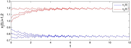
Example 4.1

Consider the below delay Nicholson's blowflies system: (58) $\begin{array}{rl}{x}_1^{\prime }(t)& =-\frac{0.6951934x_1(t)}{0.7537127+x_1(t)}+\frac{0.01x_2(t)}{0.23+x_2(t)}\\ & +(\frac{100+\sin \sqrt{2}t}{100+\cos \sqrt{7}t}+\frac{10}{1+|t|})x_1(t-(2{\mathrm{e}}^{{\sin }^{4}t}+\frac{1}{1+2|t|}))\\ & \times {\mathrm{e}}^{-(1+(100/(1+|t|)))x_1(t-(2{\mathrm{e}}^{{\sin }^{4}t}+(1/(1+2|t|))))},\\ x_2^{\prime }(t)& =-\frac{0.6951225x_2(t)}{0.7537101+x_2(t)}+\frac{0.02x_1(t)}{0.82+x_1(t)}\\ & +(\frac{100+\sin \sqrt{2}t}{100+\cos \sqrt{7}t}+\frac{10}{1+|t|})x_2(t-(2{\mathrm{e}}^{{\sin }^{4}t}+\frac{1}{1+2|t|}))\\ & \times {\mathrm{e}}^{-(1+(100/(1+|t|)))x_2(t-(2{\mathrm{e}}^{{\sin }^{4}t}+(1/(1+2|t|))))}.\end{array}$(58) Note $\tilde{\kappa }\approx 1.342276,\kappa \approx 0.7215355$. Let M = 1.31, and by some simple calculations, it is easy to verify that all the conditions of Theorem 3.1 are satisfied. Therefore, all solutions of system (58(58) $\begin{array}{rl}{x}_1^{\prime }(t)& =-\frac{0.6951934x_1(t)}{0.7537127+x_1(t)}+\frac{0.01x_2(t)}{0.23+x_2(t)}\\ & +(\frac{100+\sin \sqrt{2}t}{100+\cos \sqrt{7}t}+\frac{10}{1+|t|})x_1(t-(2{\mathrm{e}}^{{\sin }^{4}t}+\frac{1}{1+2|t|}))\\ & \times {\mathrm{e}}^{-(1+(100/(1+|t|)))x_1(t-(2{\mathrm{e}}^{{\sin }^{4}t}+(1/(1+2|t|))))},\\ x_2^{\prime }(t)& =-\frac{0.6951225x_2(t)}{0.7537101+x_2(t)}+\frac{0.02x_1(t)}{0.82+x_1(t)}\\ & +(\frac{100+\sin \sqrt{2}t}{100+\cos \sqrt{7}t}+\frac{10}{1+|t|})x_2(t-(2{\mathrm{e}}^{{\sin }^{4}t}+\frac{1}{1+2|t|}))\\ & \times {\mathrm{e}}^{-(1+(100/(1+|t|)))x_2(t-(2{\mathrm{e}}^{{\sin }^{4}t}+(1/(1+2|t|))))}.\end{array}$(58) ) are asymptotically almost periodic function on ${\mathbb{R}}^{+}$, and converge to a same almost periodic function as $t\to +\mathrm{\infty }$. These conclusions are verified by the following numerical simulations in Figure 1.

Figure 1. Numerical solutions of (58(58) $\begin{array}{rl}{x}_1^{\prime }(t)& =-\frac{0.6951934x_1(t)}{0.7537127+x_1(t)}+\frac{0.01x_2(t)}{0.23+x_2(t)}\\ & +(\frac{100+\sin \sqrt{2}t}{100+\cos \sqrt{7}t}+\frac{10}{1+|t|})x_1(t-(2{\mathrm{e}}^{{\sin }^{4}t}+\frac{1}{1+2|t|}))\\ & \times {\mathrm{e}}^{-(1+(100/(1+|t|)))x_1(t-(2{\mathrm{e}}^{{\sin }^{4}t}+(1/(1+2|t|))))},\\ x_2^{\prime }(t)& =-\frac{0.6951225x_2(t)}{0.7537101+x_2(t)}+\frac{0.02x_1(t)}{0.82+x_1(t)}\\ & +(\frac{100+\sin \sqrt{2}t}{100+\cos \sqrt{7}t}+\frac{10}{1+|t|})x_2(t-(2{\mathrm{e}}^{{\sin }^{4}t}+\frac{1}{1+2|t|}))\\ & \times {\mathrm{e}}^{-(1+(100/(1+|t|)))x_2(t-(2{\mathrm{e}}^{{\sin }^{4}t}+(1/(1+2|t|))))}.\end{array}$(58) ) for different initial values.

Remark 4.1

It is worth noting that system (58(58) $\begin{array}{rl}{x}_1^{\prime }(t)& =-\frac{0.6951934x_1(t)}{0.7537127+x_1(t)}+\frac{0.01x_2(t)}{0.23+x_2(t)}\\ & +(\frac{100+\sin \sqrt{2}t}{100+\cos \sqrt{7}t}+\frac{10}{1+|t|})x_1(t-(2{\mathrm{e}}^{{\sin }^{4}t}+\frac{1}{1+2|t|}))\\ & \times {\mathrm{e}}^{-(1+(100/(1+|t|)))x_1(t-(2{\mathrm{e}}^{{\sin }^{4}t}+(1/(1+2|t|))))},\\ x_2^{\prime }(t)& =-\frac{0.6951225x_2(t)}{0.7537101+x_2(t)}+\frac{0.02x_1(t)}{0.82+x_1(t)}\\ & +(\frac{100+\sin \sqrt{2}t}{100+\cos \sqrt{7}t}+\frac{10}{1+|t|})x_2(t-(2{\mathrm{e}}^{{\sin }^{4}t}+\frac{1}{1+2|t|}))\\ & \times {\mathrm{e}}^{-(1+(100/(1+|t|)))x_2(t-(2{\mathrm{e}}^{{\sin }^{4}t}+(1/(1+2|t|))))}.\end{array}$(58) ) is not almost periodic, and the following inequalities: (59) $\begin{array}{r}\begin{array}{rl}& \underset{t\in \mathbb{R}}{sup}{\gamma }_{ij}(t)M>30,\\ & \underset{t\in \mathbb{R}}{sup}\{-{\displaystyle \frac{a_{ii}(t)b_{ii}(t)}{(b_{ii}(t)+M{)}^2}}+\sum _{j=1,j\ne i}^2{\displaystyle \frac{a_{ij}(t)b_{ij}(t)}{(b_{ij}(t)+\kappa {)}^2}}+{\displaystyle \frac{1}{{\mathrm{e}}^2}}\sum _{j=1}^2{\beta }_{ij}(t)\}>0.4,i=1,2,\end{array}\end{array}$(59) do not meet the requirements of conditions (1.3) and (1.5) in [20,37].

To the best of our knowledge, few authors have considered the asymptotically almost periodic dynamics of Nicholson's blowflies model with both nonlinear density-dependent mortality term and patch structure. We only find [3,5,12,17–20,32–35,37,38,40] in the literature. However, all results in these papers can not be used to imply that all solutions of (58(58) $\begin{array}{rl}{x}_1^{\prime }(t)& =-\frac{0.6951934x_1(t)}{0.7537127+x_1(t)}+\frac{0.01x_2(t)}{0.23+x_2(t)}\\ & +(\frac{100+\sin \sqrt{2}t}{100+\cos \sqrt{7}t}+\frac{10}{1+|t|})x_1(t-(2{\mathrm{e}}^{{\sin }^{4}t}+\frac{1}{1+2|t|}))\\ & \times {\mathrm{e}}^{-(1+(100/(1+|t|)))x_1(t-(2{\mathrm{e}}^{{\sin }^{4}t}+(1/(1+2|t|))))},\\ x_2^{\prime }(t)& =-\frac{0.6951225x_2(t)}{0.7537101+x_2(t)}+\frac{0.02x_1(t)}{0.82+x_1(t)}\\ & +(\frac{100+\sin \sqrt{2}t}{100+\cos \sqrt{7}t}+\frac{10}{1+|t|})x_2(t-(2{\mathrm{e}}^{{\sin }^{4}t}+\frac{1}{1+2|t|}))\\ & \times {\mathrm{e}}^{-(1+(100/(1+|t|)))x_2(t-(2{\mathrm{e}}^{{\sin }^{4}t}+(1/(1+2|t|))))}.\end{array}$(58) ) converge to the almost periodic solution.

5. Conclusions

In the present paper, the issue of asymptotic almost periodicity of Nicholson's blowflies systems with nonlinear density-dependent mortality term and patch structure is investigated. The positivity, global existence and boundedness of the initial value problem on the addressed system have been shown, and the existence of the positive asymptotically almost periodic solution and its global attractivity have been established by applying Lyapunov function and analytical techniques. In particular, a numerical example is provided to illustrate these analytical conclusions. It is worth noting that our conditions are very easy to test in practice by a simple algebraic method, and the method used in this paper provides a possible approach for studying the asymptotic almost periodic dynamics of other population systems with asymptotic almost-periodic environments.

Acknowledgments

The authors would like to express the sincere appreciation to the editor and reviewers for their helpful comments in improving the presentation and quality of the paper. This work was supported by the National Natural Science Foundation of China (Nos. 11971076, 51839002,11861037), Research Promotion Program of Changsha University of Science and Technology (No. 2019QJCZ050), and the Natural Scientific Research Fund of Zhejiang Province of China (Grant No. LY18A010019).

Disclosure statement

No potential conflict of interest was reported by the author(s).

Additional information

Funding

This work was supported by the National Natural Science Foundation of China [grant numbers 11971076, 51839002,1186103], Research Promotion Program of Changsha University of Science and Technology [grant number 2019QJCZ050], and the Natural Scientific Research Fund of Zhejiang Province of China [grant number LY18A010019].

References

- L. Berezansky and E. Braverman, Boundedness and persistence of delay differential equations with mixed nonlinearity, Appl. Math. Comput. 279 (2016), pp. 154–169.
- L. Berezansky and E. Braverman, A note on stability of Mackey-Glass equations with two delays, J. Math. Anal. Appl. 450 (2017), pp. 1208–1228. doi: 10.1016/j.jmaa.2017.01.050
- L. Berezansky, E. Braverman, and L. Idels, Nicholson's blowflies differential equations revisited: main results and open problems, Appl. Math. Model. 34 (2010), pp. 1405–1417. doi: 10.1016/j.apm.2009.08.027
- Q. Cao, G. Wang, and C. Qian, New results on global exponential stability for a periodic Nicholson's blowflies model involving time-varying delays, Adv. Differ. Equ. 2020(43) (2020). Available at https://doi.org/10.1186/s13662-020-2495-4.
- W. Chen, Permanence for Nicholson-type delay systems with patch structure and nonlinear density-dependent mortality terms, Electron. J. Qual. Theory Differ. Equ. 73 (2012), pp. 1–14.
- A. Fink, Almost Periodic Differential Equations, Lecture Notes in Mathematics, Vol. 377, Springer, Berlin, 1974.
- W. Gurney, S. Blythe, and R. Nisbet, Nicholson's blowflies revisited, Nature 287 (1980), pp. 17–21. doi: 10.1038/287017a0
- J. Hale and S. Verduyn Lunel, Introduction to Functional Differential Equations, Springer, New York, 1993.
- L. Hien, Global asymptotic behaviour of positive solutions to a non-autonomous Nicholson's blowflies model with delays, J. Biol. Dyn. 8(1) (2014), pp. 135–144. doi: 10.1080/17513758.2014.917725
- C. Huang, X. Long, L. Huang, and S. Fu, Stability of almost periodic Nicholson's blowflies model involving patch structure and mortality terms, Can. Math. Bull. 63(2) (2020), pp. 405–422. doi: 10.4153/S0008439519000511
- C. Huang, Y. Qiao, L. Huang, and R. Agarwal, Dynamical behaviors of a food-chain model with stage structure and time delays, Adv. Differ. Equ. 2018 (2018), p. 3284. Available at https://doi.org/10.1186/s13662-018-1589-8.
- C. Huang, J. Wang, and L. Huang, Asymptotically almost periodicity of delayed Nicholson-type system involving patch structure, Electron. J. Differ. Equ. 2020(61) (2020), pp. 1104–17.
- C. Huang, S. Wen, M. Li, F. Wen, and X. Yang, An empirical evaluation of the influential nodes for stock market network: Chinese A shares case, Finance Res. Lett. (2020). doi: 10.1016/j.frl.2020.101517.
- C. Huang, X. Yang, and J. Cao, Stability analysis of Nicholson's blowflies equation with two different delays, Math. Comput. Simul. 171 (2020), pp. 201–206. doi: 10.1016/j.matcom.2019.09.023
- C. Huang, H Zhang, J Cao, and H Hu, Stability and Hopf bifurcation of a delayed prey-predator model with disease in the predator, Int. J. Bifurc. Chaos 29(7) (2019). 1950091. 23 pp. doi: 10.1142/S0218127419500913
- C. Huang, H. Zhang, and L. Huang, Almost periodicity analysis for a delayed Nicholson's blowflies model with nonlinear density-dependent mortality term, Commun. Pure Appl. Anal. 18(6) (2019), pp. 3337–3349. doi: 10.3934/cpaa.2019150
- B. Liu, Permanence for a delayed Nicholson's blowflies model with a nonlinear density-dependent mortality term, Ann. Polonici Math. 101(2) (2011), pp. 123–129. doi: 10.4064/ap101-2-2
- B. Liu, Almost periodic solutions for a delayed Nicholsons blowflies model with a nonlinear density-dependent mortality term, Adv. Differ. Equ. 72 (2014), pp. 1–16.
- B. Liu and S. Gong, Permanence for Nicholson-type delay systems with nonlinear density-dependent mortality terms, Nonlinear Anal. Real World Appl. 12 (2011), pp. 1931–1937. doi: 10.1016/j.nonrwa.2010.12.009
- P. Liu, L. Zhang, S. Liu, and L. Zheng, Global exponential stability of almost periodic solutions for Nicholson's Blowflies system with nonlinear density-dependent mortality terms and patch structure, Math. Model. Anal. 22(4) (2017), pp. 484–502. doi: 10.3846/13926292.2017.1329171
- X. Long and S. Gong, New results on stability of Nicholson's blowflies equation with multiple pairs of time-varying delays, Appl. Math. Lett. 100 (2020), p. 106027. Available at https://doi.org/10.1016/j.aml.2019.106027.
- Y. Muroya, Global stability for separable nonlinear delay differential equations, Comput. Math. Appl.49 (2005), pp. 1913–1927. doi: 10.1016/j.camwa.2004.02.013
- C. Qian, New periodic stability for a class of Nicholson's blowflies models with multiple different delays, Int. J. Control (2020). doi: 10.1080/00207179.2020.1766118.
- C. Qian and Y. Hu, Novel stability criteria on nonlinear density-dependent mortality Nicholson's blowflies systems in asymptotically almost periodic environments, J. Inequalities Appl. 2020(13) (2020). Available at https://doi.org/10.1186/s13660-019-2275-4.
- G. Röst and J. Wu, Domain-decomposition method for the global dynamics of delay differential equations with unimodal feedback, Proc. Royal Soc. A 463 (2007), pp. 2655–2669. doi: 10.1098/rspa.2007.1890
- B. Rothschild, Dynamics of marine fish populations, Q. Rev. Biol. 52(3) (1986), pp. 907–909.
- B. Rothschild and J. Ault, Population-dynamic instability as a cause of patch structure, Ecol. Model.93 (1996), pp. 237–249. doi: 10.1016/S0304-3800(96)00005-1
- S. Ruan, A. Ardito, P. Ricciardi, and D. Deangelis, Coexistence in competition models with density-dependent mortality (in French), Comptes Rendus Biologies 330 (2007), pp. 845–854. doi: 10.1016/j.crvi.2007.10.004
- S. Saker and S. Agarwal, Oscillation and global attractivity in a periodic Nicholson's blowflies model, Math. Comput. Model. 35 (2002), pp. 719–731. doi: 10.1016/S0895-7177(02)00043-2
- H. Smith, An Introduction to Delay Differential Equations with Applications to the Life Sciences, Springer, New York, 2011.
- J. So and J. Yu, Global attractivity and uniform persistence in Nicholson's blowflies, Differ. Equ. Dyn. Syst. 2 (1994), pp. 11–18.
- D. Son, L. HienB, and T. Anh, Global attractivity of positive periodic solution of a delayed Nicholson model with nonlinear density-dependent mortality term, Electron. J. Qual. Theory Differ. Equ. 8 (2019), pp. 1–17. doi: 10.14232/ejqtde.2019.1.62
- Y. Tang and S. Xie, Global attractivity of asymptotically almost periodic Nicholson's blowflies models with a nonlinear density-dependent mortality term, Int. J. Biomathematics 11(6) (2018), p. 1850079. 15 pp. doi: 10.1142/S1793524518500791
- W. Wang, Positive periodic solutions of delayed Nicholson's blowflies models with a nonlinear density-dependent mortality term, Appl. Math. Model. 36 (2012), pp. 4708–4713. doi: 10.1016/j.apm.2011.12.001
- W. Wang, Exponential extinction of Nicholson's blowflies system with nonlinear density-dependent mortality terms, Abstract Appl. Anal. 302065 (2012), pp. 1–17.
- J. Wei and M. Li, Hopf bifurcation analysis in a delayed Nicholson blowflies equation, Nonlinear Anal.60 (2005), pp. 1351–1367. doi: 10.1016/j.na.2003.04.002
- Y. Xu, Existence and global exponential stability of positive almost periodic solutions for a delayed Nicholson's blowflies model, J. Korean Math. Soc. 51(3) (2014), pp. 473–493. doi: 10.4134/JKMS.2014.51.3.473
- Y. Xu, New stability theorem for periodic Nicholson's model with mortality term, Appl. Math. Lett.94 (2019), pp. 59–65. doi: 10.1016/j.aml.2019.02.021
- Y. Xu, Q. Cao, and X. Guo, Stability on a patch structure Nicholson's blowflies systeminvolving distinctive delays, Appl. Math. Lett. 105 (2020), p. 106340. doi: 10.1016/j.aml.2020.106340.
- L. Yao, Dynamics of Nicholson's blowflies models with a nonlinear density-dependent mortality, Appl. Math. Model. 64 (2018), pp. 185–195. doi: 10.1016/j.apm.2018.07.007
- Z. Ye, C. Hu, L. He, G. Ouyang, and F. Wen, The dynamic time-frequency relationship between international oil prices and investor sentiment in China: A wavelet coherence analysis, Energy J. 41(01) (2020). doi:10.5547/01956574.41.5.fwen.
- T. Yi and X. Zou, Global attractivity of the diffusive Nicholson blowflies equation with Neumann boundary condition: A non-monotone case, J. Differ. Equ. 245(11) (2008), pp. 3376–3388. doi: 10.1016/j.jde.2008.03.007
- C. Zhang, Almost Periodic Type Functions and Ergodicity, Kluwer Academic/Science Press, Beijing, 2003.