A stochastic SACR epidemic model for HBV transmission

Abstract

In this article, a stochastic SACR hepatitis B epidemic model is taken to be under consideration. We develop a stochastic epidemic model by considering the effect of environmental fluctuation on the hepatitis B dynamics and distribute the transmission rate by white noise. Using the stochastic Lyapunov function theory, we have shown the existence and uniqueness of the global positive solution. The extinction and persistence for our proposed model are derived with sufficient conditions. The numerical simulations are carried out using first-order Itô-Taylor stochastic scheme in the last section for the verification of our theoretical results.

Keywords:

• Hepatitis B
• stochastic epidemic model
• existence and uniqueness
• extinction and persistence
• numerical simulation

1. Introduction

Environmental noise and environmental variation play an effective role in the transmission of infectious diseases. Dengue, hepatitis B and Malaria, etc., are some of the best examples. Epidemic and spread of infectious diseases are random due to the unpredictable contacts of one individual to another individual [1, 2]. In this sense, environmental fluctuations have a critical influence on the epidemic development [18, 21]. Hence this randomness of the environment enters into the state of the epidemic. Such an unpredictable influence of the environment can be seen in the epidemic growth and spreads of contagious disease of hepatitis B, caused by hepatitis B viral infection since individual to individual contact is random [4]. The variability and randomness of the environment are fed through the state of the epidemics [21]. And in epidemic dynamics, stochastic models may be a more appropriate way of modelling epidemics in many circumstances. For example, stochastic models can take care of randomness of the infectious contacts occurring in the infectious periods [3].

Hepatitis B is a contagious disease that causes the liver's inflammation, which results from the Hepatitis B virus infection. HBV is not cytopathic. It should be noted that HBV hijacks host machinery and results in cancerous cells. Most likely it damages hepatocyte and does not kill host cells itself, however, the reaction to the invulnerable system aggression will lead to liver inflammation. After entering into the body, HBV infects the hepatocyte cells in the liver. The immune system in response to such infection conduces to irritation of the liver. Most hepatitis infections are caused by a virus, infection, due to bacteria or active exposure to alcohol and drugs. Two thousand years ago, the hepatitis B virus was first observed by Hippocrates. Hepatitis B virus is considered as one of the fatal infections due to which millions of people have died. Hepatitis B virus infects the liver of the human body and is the main cause of liver cancer. The transmission of the hepatitis B virus from infected to susceptible people is vertical as well horizontal. Hepatitis B is divided into two stages i.e acute and chronic. The acute stage consists of the first few months normally considered as six months after exposure to the virus, during which the immune system of the human body is capable to control the infection. Feeling sick and high temperature are the two main symptoms of the acute stage, which fade away after some weeks due to the immune system. The chronic stage is the worst stage in which the liver fails to function properly and cancer cells develop. The treatment of a person in the chronic stage takes several years.

Mathematical modelling is considered an effective tool for describing the dynamic behaviour of infections. For realizing and controlling the outbreak of transmissible diseases in a group, many researchers have formulated models. The application of mathematical modelling has been in vogue for the study of transmissible infectious diseases. Epidemic models of two types are identified by deterministic and stochastic. The most effective epidemic model for such type is the stochastic one because it results in a larger degree of realism between evaluation in imitation. The stochastic one gives us more valuable output with a comparison to the deterministic model. By executing the stochastic model various times, we can make a distribution of outcomes. To study the dynamics of various infectious diseases, mathematical modelling is considered as one of the best techniques to formulate the phenomenon in the system of equations. Several researchers have worked on different infectious diseases. They have developed different mathematical models for these epidemic diseases, and then studied the stability analysis and optimal control of these epidemic models (see e.g. [17, 19, 20, 25, 28, 31]), which not only helps in the control/spread of infectious diseases but also helps in prevention of these diseases in daily life. Modelling of epidemic models is helpful to academia as well as to daily life. Epidemic models are broadly classified into two categories i.e deterministic and stochastic. The stochastic models have an advantage over the deterministic models as these models are very close to nature and depict exact biological phenomena [5]. In explicating many fields of natural and engineering sciences, the role of stochastic models is pivotal. In medical and biological processes, the inherent variability can be studied using stochastic models k [7, 9, 14, 15, 30]. They can be used to counter (i) the risk effects in managerial economics (ii) psychological complexities and (iii) fluctuation in rates. Many researchers have worked on stochastic epidemic models to analyse and control different diseases i.e Hepatitis B, avian influenza, leishmaniasis, tuberculosis, etc. [6, 12, 13, 16, 26, 32].

As most real-world problems are not deterministic, including stochastic effects into the model gives us a more realistic way of modelling dynamics. Population systems are often subject to environmental noise which is ignored by the deterministic models. Hence the stochastic model has come to play an important role in infectious dynamics. Modelling the biological phenomena stochastic differential equation is more reasonable than deterministic [5]. To reflect the actual problem as much as possible, many mathematical researchers and biologists have long been interested in the stochastic effects that may lead to significant changes. Stochastic models produce more valuable output than deterministic models as by running a stochastic model several times, we can build up a distribution of the predicted outcomes, e.g. the number of infected classes at the time t, whereas a deterministic model, will just give a single predicted value [7–9, 14, 29, 30]. Many epidemic models have been discovered for the description of viral dynamic of hepatitis B, which are mostly using the deterministic approach (see for detail [6, 12, 13, 26, 32]). Recently Khan et al. [11] presented a stochastic model for the transmission dynamics of hepatitis B.

The study is focused on a stochastic hepatitis B epidemic model, keeping in view the nature of varying populations for the behaviour of long duration by extending the work of Khan et al. [11] to discuss both the acute and chronic stages of hepatitis B stochastic epidemic model. The total population is classified into four groups. The susceptible class composes of those people who are not infected yet and white noise distributes the transmission rate. The infected (acute) class consists of those individuals who are infected but they cannot transfer the virus to other individuals. The third class consists of chronic individuals and the fourth class includes recovered individuals. We derive sufficient conditions for disease extinction and persistence. We illustrate numerical simulation to support our theoretical findings by using the stochastic Milstein scheme method, see [23, 24].

Literature reveals that very few attempts have been established by the researchers using hepatitis B stochastic epidemic model. That is why; in this paper we made an attempt to show the considerable effect of a stochastic factor on the SACR dynamics with acute and chronic stages.

2. Formulation of the model

Therefore, motivated by the aforementioned work, we study the stochastic hepatitis B epidemic model with varying population environment. We put the following assumption on the epidemic model:

(A1)	The total population $N\left(t\right)$ at time t is divided into four compartments: the susceptible individuals, $S\left(t\right)$, the acutely infected with hepatitis B individuals, $A\left(t\right)$, the chronically infected with hepatitis B individuals, $C\left(t\right)$ and the recovered individuals, $R\left(t\right)$, i.e. $N\left(t\right)=S\left(t\right)+A\left(t\right)+C\left(t\right)+R\left(t\right)$ varies with time t.
(A2)	All parameters and state variables of the proposed model are non-negative.
(A3)	For the effect of randomly fluctuating environment taking, $\alpha \to \alpha +\sigma \dot{\phantom{a}}B\left(t\right)$, where ${\sigma }^2>0$ denotes the intensity of white noise and $B\left(t\right)$ represents the standard Brownian motion satisfying the condition $B\left(0\right)=0$.

The assumption $\left(A_1\right)$–$\left(A_3\right)$ leads to the stochastic hepatitis B epidemic model, which is represented by the following system of four stochastic differential equations: (1) $\begin{array}{rl}\mathrm{d}S\left(t\right)& =(b-\alpha S\left(t\right)C\left(t\right)-(v+{\mu }_0)S\left(t\right))\mathrm{d}t-\sigma S\left(t\right)C\left(t\right)\mathrm{d}B\left(t\right),\\ \mathrm{d}A\left(t\right)& =(\alpha S\left(t\right)C\left(t\right)-({\gamma }_1+{\mu }_0+\text{β})A\left(t\right))\mathrm{d}t+\sigma S\left(t\right)C\left(t\right)\mathrm{d}B\left(t\right),\\ \mathrm{d}C\left(t\right)& =(\text{β}A\left(t\right)-({\gamma }_2+{\mu }_0+{\mu }_1)C\left(t\right))\mathrm{d}t,\\ \mathrm{d}R\left(t\right)& =vS\left(t\right)+({\gamma }_{2}C\left(t\right)-{\mu }_{0}R\left(t\right)+{\gamma }_{1}A\left(t\right))\mathrm{d}t.\end{array}$(1) By putting $\sigma =0$, we get the deterministic model as (2) $\begin{array}{rl}\mathrm{d}S\left(t\right)& =(b-\alpha S\left(t\right)C\left(t\right)-(v+{\mu }_0)S\left(t\right))\mathrm{d}t,\\ \mathrm{d}A\left(t\right)& =(\alpha S\left(t\right)C\left(t\right)-({\gamma }_1+{\mu }_0+\text{β})A\left(t\right))\mathrm{d}t,\\ \mathrm{d}C\left(t\right)& =(\text{β}A\left(t\right)-({\gamma }_2+{\mu }_0+{\mu }_1)C\left(t\right))\mathrm{d}t,\\ \mathrm{d}R\left(t\right)& =vS\left(t\right)+({\gamma }_{2}C\left(t\right)-{\mu }_{0}R\left(t\right)+{\gamma }_{1}A\left(t\right))\mathrm{d}t.\end{array}$(2) The basic reproduction number of the deterministic model is (3) $R_0^d=\frac{\alpha \text{β}b}{\left({\mu }_0+v\right)\left({\mu }_0+\text{β}+{\gamma }_1\right)\left({\mu }_0+{\mu }_1+{\gamma }_2\right)}.$(3) The parameters description with their units is presented in Table 1.

Table 1. Parameters value.

Notation	Parameter description	Value	Source
b	The constant birth rate	0.5	[11]
α	The transmission rate	0.6, 0.36 ${\mathrm{d}\mathrm{a}\mathrm{y}}^{-1}$	[11]
${\mu }_0$	Natural death rate	0.5	[11]
${\mu }_1$	The disease induced death rate	0.2 ${\mathrm{d}\mathrm{a}\mathrm{y}}^{-1}$	[11]
v	The vaccination rate	0.01	[11]
${\gamma }_1$	The constant recovery rate for acutely infected individuals	0.2, 0.4 ${\mathrm{d}\mathrm{a}\mathrm{y}}^{-1}$	[11]
${\gamma }_2$	The constant recovery rate for chronically infected individuals	0.4, 0.2 ${\mathrm{d}\mathrm{a}\mathrm{y}}^{-1}$	[11]
β	The moving rate of acutely infected individuals to chronic stage	0.1, 0.4 ${\mathrm{d}\mathrm{a}\mathrm{y}}^{-1}$	[11]

3. Existence and uniqueness

By proving the following theorem, we show existence and uniqueness of our model (1(1) $\begin{array}{rl}\mathrm{d}S\left(t\right)& =(b-\alpha S\left(t\right)C\left(t\right)-(v+{\mu }_0)S\left(t\right))\mathrm{d}t-\sigma S\left(t\right)C\left(t\right)\mathrm{d}B\left(t\right),\\ \mathrm{d}A\left(t\right)& =(\alpha S\left(t\right)C\left(t\right)-({\gamma }_1+{\mu }_0+\text{β})A\left(t\right))\mathrm{d}t+\sigma S\left(t\right)C\left(t\right)\mathrm{d}B\left(t\right),\\ \mathrm{d}C\left(t\right)& =(\text{β}A\left(t\right)-({\gamma }_2+{\mu }_0+{\mu }_1)C\left(t\right))\mathrm{d}t,\\ \mathrm{d}R\left(t\right)& =vS\left(t\right)+({\gamma }_{2}C\left(t\right)-{\mu }_{0}R\left(t\right)+{\gamma }_{1}A\left(t\right))\mathrm{d}t.\end{array}$(1) )

Theorem 3.1

The solution $\left(S\right(t),A(t),C(t),R(t\left)\right)$ of model (1(1) $\begin{array}{rl}\mathrm{d}S\left(t\right)& =(b-\alpha S\left(t\right)C\left(t\right)-(v+{\mu }_0)S\left(t\right))\mathrm{d}t-\sigma S\left(t\right)C\left(t\right)\mathrm{d}B\left(t\right),\\ \mathrm{d}A\left(t\right)& =(\alpha S\left(t\right)C\left(t\right)-({\gamma }_1+{\mu }_0+\text{β})A\left(t\right))\mathrm{d}t+\sigma S\left(t\right)C\left(t\right)\mathrm{d}B\left(t\right),\\ \mathrm{d}C\left(t\right)& =(\text{β}A\left(t\right)-({\gamma }_2+{\mu }_0+{\mu }_1)C\left(t\right))\mathrm{d}t,\\ \mathrm{d}R\left(t\right)& =vS\left(t\right)+({\gamma }_{2}C\left(t\right)-{\mu }_{0}R\left(t\right)+{\gamma }_{1}A\left(t\right))\mathrm{d}t.\end{array}$(1) ) is unique for an initial value $\xi \left(0\right)=\left(S\right(0),A(0),C(0),R(0\left)\right)\in R_{+}^4,$ where $t\ge 0$. Also, $\xi \left(t\right)=\left(S\right(t),A(t),C(t),R(t\left)\right)\in R_{+}^4$ for all $t\ge 0$ i.e. the solution lies in $R_{+}^4$ with probability 1 a.s (almost surely).

Proof.

For any $\xi \left(0\right)\in R_{+}^4$, the locally Lipschitz condition is clearly satisfied by the coefficients of our model. Consequently, a unique local solution $\xi \left(t\right)$ exists on $t\in [0,{\tau }_e)$, ${\tau }_e$ represents the explosion time [5, 6]. Now, we have to show that the solution exists globally as well, and for this we will show that ${\tau }_e=\mathrm{\infty }$ a.s. For a sufficiently large value $k_0\ge 0$, $S\left(0\right)$, $A\left(0\right)$, $C\left(0\right)$ and $R\left(0\right)$ remains in $[\frac{1}{k_0},k_0]$. For all integer $k\ge k_0$, let us consider the stopping time as (4) ${\tau }_k=\left\{t\in [0,{\tau }_e):max\left\{S\right(t),A(t),C(t),R(t\left)\right\}\ge k\mathrm{o}\mathrm{r}min\left\{S\left(t\right),A\left(t\right),C\left(t\right),R\left(t\right)\le \frac{1}{k}\right\}\right\}.$(4) Similarly to the work of [22], we use the notion $inf\phi =\mathrm{\infty }$ thought in this study, where φ is an empty set. ${\tau }_k$ increases as k approaches to ∞. The setting of ${\tau }_{\mathrm{\infty }}=\underset{k\to \mathrm{\infty }}{lim}$ along with the use of ${\tau }_{\mathrm{\infty }}\le {\tau }_e$ a.s proves that ${\tau }_{\mathrm{\infty }}$ is $=\mathrm{\infty }$ a.s., and the solution of (1(1) $\begin{array}{rl}\mathrm{d}S\left(t\right)& =(b-\alpha S\left(t\right)C\left(t\right)-(v+{\mu }_0)S\left(t\right))\mathrm{d}t-\sigma S\left(t\right)C\left(t\right)\mathrm{d}B\left(t\right),\\ \mathrm{d}A\left(t\right)& =(\alpha S\left(t\right)C\left(t\right)-({\gamma }_1+{\mu }_0+\text{β})A\left(t\right))\mathrm{d}t+\sigma S\left(t\right)C\left(t\right)\mathrm{d}B\left(t\right),\\ \mathrm{d}C\left(t\right)& =(\text{β}A\left(t\right)-({\gamma }_2+{\mu }_0+{\mu }_1)C\left(t\right))\mathrm{d}t,\\ \mathrm{d}R\left(t\right)& =vS\left(t\right)+({\gamma }_{2}C\left(t\right)-{\mu }_{0}R\left(t\right)+{\gamma }_{1}A\left(t\right))\mathrm{d}t.\end{array}$(1) ) lie in $R_{+}^4$ a.s., ∀ $t\ge 0$. Also for the completion of conclusion, we will prove ${\tau }_e=\mathrm{\infty }$ a.s. If this is is not true, then constants pair exists for T>0 and $ϵ\in (0,1)$, so that (5) $P\{{\tau }_k\le T\}\ge ϵ.$(5) Consequently, we can find $k_1\in Z$ so that $P\{{\tau }_k\le T\}\ge ϵ,\mathrm{f}\mathrm{o}\mathrm{r}\mathrm{a}\mathrm{l}\mathrm{l}k\ge k_1.$ Now, let $N\left(t\right)=S\left(t\right)+A\left(t\right)+C\left(t\right)+R\left(t\right)$ and for all $t\le {\tau }_k$, we have (6) $\mathrm{d}N\left(t\right)=(b-{\mu }_{1}C\left(t\right)-{\mu }_{0}N\left(t\right))\mathrm{d}t\le (b-{\mu }_{0}N\left(t\right))\mathrm{d}t.$(6) By calculating  Equation (6(6) $\mathrm{d}N\left(t\right)=(b-{\mu }_{1}C\left(t\right)-{\mu }_{0}N\left(t\right))\mathrm{d}t\le (b-{\mu }_{0}N\left(t\right))\mathrm{d}t.$(6) ), one can derive that (7) $N\left(t\right)\le \left\{\begin{array}{ll}\frac{b}{{\mu }_0},& \mathrm{i}\mathrm{f}N\left(0\right)\le \frac{b}{{\mu }_0},\\ N\left(0\right),& \mathrm{i}\mathrm{f}N\left(0\right)>\frac{b}{{\mu }_0},\end{array}\right.:=M.$(7) We define a function $G\in C^2$, $G:R_{+}^4\to R_{+}$, satisfying (8) $G(S,A,C,R)=-(\log R+\log A+\log C+\log S)+S+A+C+R-1.$(8) Since we know that $logy\le y-1$ for all 0<y, therefore G is clearly non-negative. Consider $k\ge k_0$, T>0 and using $It\hat{o}$ formula to Equation (8(8) $G(S,A,C,R)=-(\log R+\log A+\log C+\log S)+S+A+C+R-1.$(8) ), we obtain (9) $\begin{array}{rl}\mathrm{d}G(S,A,C,R)& =\frac{1}{2S^2}(\mathrm{d}S{)}^2+\left(1-\frac{1}{S}\right)\mathrm{d}S+\left(1-\frac{1}{R}\right)\mathrm{d}R+\left(1-\frac{1}{C}\right)\mathrm{d}C\\ & +\frac{1}{2A^2}(\mathrm{d}A{)}^2+\left(1-\frac{1}{A}\right)\mathrm{d}A,\\ & =LG(S,A,C,R)\mathrm{d}t+\sigma (I-S)\mathrm{d}B\left(t\right),\end{array}$(9) where $LG(R,C,A,S):R_{+}^4\to R_{+}$ is (10) $\begin{array}{rl}LG(S,A,C,R)& =\left(1-\frac{1}{S}\right)\left(b-\alpha S\left(t\right)C\left(t\right)-(v+{\mu }_0)S\left(t\right)\right)+\frac{1}{2}{\sigma }^2{I}^2\\ & +\left(1-\frac{1}{A}\right)\left(\alpha S\left(t\right)C\left(t\right)-(\text{β}+{\gamma }_1+{\mu }_0)A\left(t\right)\right)+\frac{1}{2}{\sigma }^2{S}^2\\ & +\left(1-\frac{1}{C}\right)\left(-({\gamma }_2+{\mu }_1+{\mu }_0)C\left(t\right)+\text{β}A\left(t\right)\right)\\ & +\left(1-\frac{1}{R}\right)\left(vS\left(t\right)-{\mu }_{0}R\left(t\right)+{\gamma }_{1}A\left(t\right)+{\gamma }_{2}C\left(t\right)\right)\\ & =b-(v+{\mu }_0)S-\frac{b}{S}+\alpha C+{\mu }_0+v+\frac{1}{2}{\sigma }^2{I}^2\\ & -({\gamma }_1+{\mu }_0+\text{β})A-\alpha \frac{SC}{A}+{\gamma }_1+{\mu }_0+\text{β}+\frac{1}{2}{\sigma }^2{S}^2\\ & +\text{β}A-({\gamma }_2+{\mu }_0+{\mu }_1)C-\text{β}\frac{A}{C}+{\mu }_0+{\mu }_1+{\gamma }_2\\ & +{\gamma }_{1}A+{\gamma }_{2}C-{\mu }_{0}R+vS-{\gamma }_1\frac{A}{R}-{\gamma }_2\frac{C}{R}+{\mu }_0-v\frac{S}{R},\\ & \le b+\alpha C+v+{\mu }_0+{\mu }_0+\text{β}+{\gamma }_1+\frac{1}{2}{\sigma }^2(I^2+S^2)\\ & +\text{β}A+{\mu }_1+{\mu }_0+{\gamma }_2\\ & +{\gamma }_{1}A+{\gamma }_{2}C+vS+{\mu }_0,\\ & \le b+4{\mu }_0+v+{\sigma }^2{M}^2+(\alpha +\text{β}+{\gamma }_1+{\gamma }_2+v)M+\text{β}+{\mu }_1\\ & +{\gamma }_1+{\gamma }_2:=K.\end{array}$(10) Hence (11) $\begin{array}{rl}E\left[G\left(R\right({\tau }_k\wedge T),C({\tau }_k\wedge T),A({\tau }_k\wedge T),S({\tau }_k\wedge T\left)\right)\right]& \le G\left(\xi \right(0\left)\right)+E\left[{\int }_0^{{\tau }_k\wedge T}K\mathrm{d}t\right],\\ & \le G\left(\xi \right(0\left)\right)+KT.\end{array}$(11) For all $k\ge k_1$ let ${\tau }_k\le T={\mathrm{\Omega }}_k$ then $P\left({\mathrm{\Omega }}_k\right)\ge ϵ$, by using corresponding to each $\omega \in {\mathrm{\Omega }}_k$, we can find $R({\tau }_k,\omega )$, $C({\tau }_k,\omega )$,$A({\tau }_k,\omega )$, $S({\tau }_k,\omega )$, whose value is either $\frac{1}{k}$ or k, consequently, $G\left(R\right({\tau }_k),C({\tau }_k),A({\tau }_k),S({\tau }_k\left)\right)$ is not less than $\log k+\frac{1}{k}-1$ or $k-1-\log k$. So (12) $G\left(R\right({\tau }_k),C({\tau }_k),A({\tau }_k),S({\tau }_k\left)\right)\ge E\left(\log k+\frac{1}{k}-1\right)\wedge \left(k-1-\log k\right).$(12) Taking into account Equation (5(5) $P\{{\tau }_k\le T\}\ge ϵ.$(5) ) and  Equation (11(11) $\begin{array}{rl}E\left[G\left(R\right({\tau }_k\wedge T),C({\tau }_k\wedge T),A({\tau }_k\wedge T),S({\tau }_k\wedge T\left)\right)\right]& \le G\left(\xi \right(0\left)\right)+E\left[{\int }_0^{{\tau }_k\wedge T}K\mathrm{d}t\right],\\ & \le G\left(\xi \right(0\left)\right)+KT.\end{array}$(11) ), we have (13) $\begin{array}{rl}G\left(\xi \right(0\left)\right)+KT& \ge E\left[1_{\mathrm{\Omega }\left(\omega \right)}G\left(R\left({\tau }_k\right),C\left({\tau }_k\right),A\left({\tau }_k\right),S\left({\tau }_k\right)\right)\right]\\ & \ge ϵ\left[\left(\log k+\frac{1}{k}-1\right)\wedge \left(k-1-\log k\right)\right].\end{array}$(13) The indicator function of Ω is denoted by $1_{\mathrm{\Omega }\left(\omega \right)}$. As k approaches to ∞ the contradiction arises, i.e $\mathrm{\infty }>G\left(\xi \right(0\left)\right)+MT=\mathrm{\infty }$, hence ${\tau }_{\mathrm{\infty }}$ is equal to infinity a.s.

Remark 3.1

From Theorem 3.1 it is concluded that for any $\xi \left(0\right)\in R_{+}^4$, there is $\left(\xi \right(t\left)\right)\in R_{+}^4$ i.e a unique global solution exist a.s. of model (1(1) $\begin{array}{rl}\mathrm{d}S\left(t\right)& =(b-\alpha S\left(t\right)C\left(t\right)-(v+{\mu }_0)S\left(t\right))\mathrm{d}t-\sigma S\left(t\right)C\left(t\right)\mathrm{d}B\left(t\right),\\ \mathrm{d}A\left(t\right)& =(\alpha S\left(t\right)C\left(t\right)-({\gamma }_1+{\mu }_0+\text{β})A\left(t\right))\mathrm{d}t+\sigma S\left(t\right)C\left(t\right)\mathrm{d}B\left(t\right),\\ \mathrm{d}C\left(t\right)& =(\text{β}A\left(t\right)-({\gamma }_2+{\mu }_0+{\mu }_1)C\left(t\right))\mathrm{d}t,\\ \mathrm{d}R\left(t\right)& =vS\left(t\right)+({\gamma }_{2}C\left(t\right)-{\mu }_{0}R\left(t\right)+{\gamma }_{1}A\left(t\right))\mathrm{d}t.\end{array}$(1) ), such that (14) $\mathrm{d}N\left(t\right)\le (b-{\mu }_{0}N\left(t\right)).$(14) Simplification leads to (15) $\left(N\left(0\right)-\frac{b}{{\mu }_0}\right)\left(b-{\mu }_{0}N\left(t\right)\right)e^{-{\mu }_{0}t}+\frac{b}{{\mu }_0}\ge N\left(t\right).$(15) If $\frac{b}{{\mu }_0}\ge N\left(0\right)$, then $\frac{b}{{\mu }_0}\ge N\left(t\right)$ a.s, so (16) ${\mathrm{\Omega }}^{\ast }=\{(S,A,C,R):S>0,R\ge 0,C\ge 0,A\ge 0,\frac{b}{{\mu }_0}\ge N\},$(16)

supposing that $\xi \left(0\right)\in {\mathrm{\Omega }}^{\ast }$ always.

4. Extinction and persistence

To show conditions for extinction and persistence of the model (1(1) $\begin{array}{rl}\mathrm{d}S\left(t\right)& =(b-\alpha S\left(t\right)C\left(t\right)-(v+{\mu }_0)S\left(t\right))\mathrm{d}t-\sigma S\left(t\right)C\left(t\right)\mathrm{d}B\left(t\right),\\ \mathrm{d}A\left(t\right)& =(\alpha S\left(t\right)C\left(t\right)-({\gamma }_1+{\mu }_0+\text{β})A\left(t\right))\mathrm{d}t+\sigma S\left(t\right)C\left(t\right)\mathrm{d}B\left(t\right),\\ \mathrm{d}C\left(t\right)& =(\text{β}A\left(t\right)-({\gamma }_2+{\mu }_0+{\mu }_1)C\left(t\right))\mathrm{d}t,\\ \mathrm{d}R\left(t\right)& =vS\left(t\right)+({\gamma }_{2}C\left(t\right)-{\mu }_{0}R\left(t\right)+{\gamma }_{1}A\left(t\right))\mathrm{d}t.\end{array}$(1) ), we define some preliminaries which will be used in our main results. Let us define $⟨y\left(t\right)⟩=\frac{1}{t}{\int }_0^{t}y\left(r\right)\mathrm{d}r,$ and (17) $R_0=\frac{b\alpha }{(v+{\mu }_0)({\gamma }_1+{\mu }_0+\text{β}+\frac{1}{2}{\sigma }^2{S}_0)}.$(17)

Definition 4.1

[27]

The condition for the model (1(1) $\begin{array}{rl}\mathrm{d}S\left(t\right)& =(b-\alpha S\left(t\right)C\left(t\right)-(v+{\mu }_0)S\left(t\right))\mathrm{d}t-\sigma S\left(t\right)C\left(t\right)\mathrm{d}B\left(t\right),\\ \mathrm{d}A\left(t\right)& =(\alpha S\left(t\right)C\left(t\right)-({\gamma }_1+{\mu }_0+\text{β})A\left(t\right))\mathrm{d}t+\sigma S\left(t\right)C\left(t\right)\mathrm{d}B\left(t\right),\\ \mathrm{d}C\left(t\right)& =(\text{β}A\left(t\right)-({\gamma }_2+{\mu }_0+{\mu }_1)C\left(t\right))\mathrm{d}t,\\ \mathrm{d}R\left(t\right)& =vS\left(t\right)+({\gamma }_{2}C\left(t\right)-{\mu }_{0}R\left(t\right)+{\gamma }_{1}A\left(t\right))\mathrm{d}t.\end{array}$(1) ) is persistent in mean, if $\underset{t\to \mathrm{\infty }}{lim}inf{\int }_0^{t}A\left(r\right)\mathrm{d}r>0\mathrm{a}.\mathrm{s}.$

4.1. Extinction

We now prove our main result i.e to show the conditions for which extinction of model (1(1) $\begin{array}{rl}\mathrm{d}S\left(t\right)& =(b-\alpha S\left(t\right)C\left(t\right)-(v+{\mu }_0)S\left(t\right))\mathrm{d}t-\sigma S\left(t\right)C\left(t\right)\mathrm{d}B\left(t\right),\\ \mathrm{d}A\left(t\right)& =(\alpha S\left(t\right)C\left(t\right)-({\gamma }_1+{\mu }_0+\text{β})A\left(t\right))\mathrm{d}t+\sigma S\left(t\right)C\left(t\right)\mathrm{d}B\left(t\right),\\ \mathrm{d}C\left(t\right)& =(\text{β}A\left(t\right)-({\gamma }_2+{\mu }_0+{\mu }_1)C\left(t\right))\mathrm{d}t,\\ \mathrm{d}R\left(t\right)& =vS\left(t\right)+({\gamma }_{2}C\left(t\right)-{\mu }_{0}R\left(t\right)+{\gamma }_{1}A\left(t\right))\mathrm{d}t.\end{array}$(1) ) holds.

Theorem 4.1

Let the solution of (1(1) $\begin{array}{rl}\mathrm{d}S\left(t\right)& =(b-\alpha S\left(t\right)C\left(t\right)-(v+{\mu }_0)S\left(t\right))\mathrm{d}t-\sigma S\left(t\right)C\left(t\right)\mathrm{d}B\left(t\right),\\ \mathrm{d}A\left(t\right)& =(\alpha S\left(t\right)C\left(t\right)-({\gamma }_1+{\mu }_0+\text{β})A\left(t\right))\mathrm{d}t+\sigma S\left(t\right)C\left(t\right)\mathrm{d}B\left(t\right),\\ \mathrm{d}C\left(t\right)& =(\text{β}A\left(t\right)-({\gamma }_2+{\mu }_0+{\mu }_1)C\left(t\right))\mathrm{d}t,\\ \mathrm{d}R\left(t\right)& =vS\left(t\right)+({\gamma }_{2}C\left(t\right)-{\mu }_{0}R\left(t\right)+{\gamma }_{1}A\left(t\right))\mathrm{d}t.\end{array}$(1) ) be $\xi \left(t\right)$ with $\xi \left(0\right)\in {\mathrm{\Omega }}^{\ast }$. If

1. $\alpha ({\mu }_0+v)>{\sigma }^{2}b$ and $1>R_0$, then $\underset{t\to \mathrm{\infty }}{lim}\left(\frac{\log A\left(t\right)}{t}\right)<0,$ moreover (18) $\underset{t\to \mathrm{\infty }}{lim}S\left(t\right)=S^0,\underset{t\to \mathrm{\infty }}{lim}A\left(t\right)=0,\underset{t\to \mathrm{\infty }}{lim}C\left(t\right)=0,\underset{t\to \mathrm{\infty }}{lim}R\left(t\right)=R^0.$(18)

Proof.

Taking integration of (1(1) $\begin{array}{rl}\mathrm{d}S\left(t\right)& =(b-\alpha S\left(t\right)C\left(t\right)-(v+{\mu }_0)S\left(t\right))\mathrm{d}t-\sigma S\left(t\right)C\left(t\right)\mathrm{d}B\left(t\right),\\ \mathrm{d}A\left(t\right)& =(\alpha S\left(t\right)C\left(t\right)-({\gamma }_1+{\mu }_0+\text{β})A\left(t\right))\mathrm{d}t+\sigma S\left(t\right)C\left(t\right)\mathrm{d}B\left(t\right),\\ \mathrm{d}C\left(t\right)& =(\text{β}A\left(t\right)-({\gamma }_2+{\mu }_0+{\mu }_1)C\left(t\right))\mathrm{d}t,\\ \mathrm{d}R\left(t\right)& =vS\left(t\right)+({\gamma }_{2}C\left(t\right)-{\mu }_{0}R\left(t\right)+{\gamma }_{1}A\left(t\right))\mathrm{d}t.\end{array}$(1) ) we get (19) $\begin{array}{rl}\frac{S\left(t\right)-S\left(0\right)}{t}& =b-\alpha ⟨S\left(t\right)C\left(t\right)⟩-(v+{\mu }_0)⟨S\left(t\right)⟩-\frac{\sigma }{t}{\int }_0^{t}S\left(r\right)C\left(r\right)\mathrm{d}B\left(r\right),\\ \frac{A\left(t\right)-A\left(0\right)}{t}& =\alpha ⟨S\left(t\right)C\left(t\right)⟩-({\gamma }_1+{\mu }_0+\text{β})⟨A\left(t\right)⟩+\frac{\sigma }{t}{\int }_0^{t}S\left(r\right)C\left(r\right)\mathrm{d}B\left(r\right),\\ \frac{C\left(t\right)-C\left(0\right)}{t}& =\text{β}⟨A\left(t\right)⟩-({\gamma }_2+{\mu }_0+{\mu }_1)⟨C\left(t\right)⟩,\\ \frac{R\left(t\right)-R\left(0\right)}{t}& ={\gamma }_1⟨A\left(t\right)⟩+v⟨S\left(t\right)⟩-{\mu }_0⟨R\left(t\right)⟩+{\gamma }_2⟨C\left(t\right)⟩.\end{array}$(19) Simplify Equation (19(19) $\begin{array}{rl}\frac{S\left(t\right)-S\left(0\right)}{t}& =b-\alpha ⟨S\left(t\right)C\left(t\right)⟩-(v+{\mu }_0)⟨S\left(t\right)⟩-\frac{\sigma }{t}{\int }_0^{t}S\left(r\right)C\left(r\right)\mathrm{d}B\left(r\right),\\ \frac{A\left(t\right)-A\left(0\right)}{t}& =\alpha ⟨S\left(t\right)C\left(t\right)⟩-({\gamma }_1+{\mu }_0+\text{β})⟨A\left(t\right)⟩+\frac{\sigma }{t}{\int }_0^{t}S\left(r\right)C\left(r\right)\mathrm{d}B\left(r\right),\\ \frac{C\left(t\right)-C\left(0\right)}{t}& =\text{β}⟨A\left(t\right)⟩-({\gamma }_2+{\mu }_0+{\mu }_1)⟨C\left(t\right)⟩,\\ \frac{R\left(t\right)-R\left(0\right)}{t}& ={\gamma }_1⟨A\left(t\right)⟩+v⟨S\left(t\right)⟩-{\mu }_0⟨R\left(t\right)⟩+{\gamma }_2⟨C\left(t\right)⟩.\end{array}$(19) ), that (20) $\begin{array}{rl}& \frac{C\left(t\right)-C\left(0\right)}{t}+\frac{A\left(t\right)-A\left(0\right)}{t}+\frac{S\left(t\right)-S\left(0\right)}{t}\\ & =b-(v+{\mu }_0)⟨S\left(t\right)⟩-({\gamma }_1+{\mu }_0)⟨A\left(t\right)⟩-({\gamma }_2+{\mu }_1+{\mu }_0)⟨C\left(t\right)⟩,\end{array}$(20) (21) $\begin{array}{rl}& ⟨S\left(t\right)⟩=\frac{b}{v+{\mu }_0}-⟨A\left(t\right)⟩\frac{{\gamma }_1+{\mu }_0}{v+{\mu }_0}-⟨C\left(t\right)⟩\frac{{\mu }_1+{\gamma }_2+{\mu }_0}{v+{\mu }_0}+\phi \left(t\right)\\ & \phi \left(t\right)=-\frac{1}{v+{\mu }_0}\left[\frac{C\left(t\right)-C\left(0\right)}{t}+\frac{A\left(t\right)-A\left(0\right)}{t}+\frac{S\left(t\right)-S\left(0\right)}{t}\right].\end{array}$(21) Clearly $\phi \left(t\right)\to 0$ as $t\to \mathrm{\infty }$. Considering the second equation of model (1(1) $\begin{array}{rl}\mathrm{d}S\left(t\right)& =(b-\alpha S\left(t\right)C\left(t\right)-(v+{\mu }_0)S\left(t\right))\mathrm{d}t-\sigma S\left(t\right)C\left(t\right)\mathrm{d}B\left(t\right),\\ \mathrm{d}A\left(t\right)& =(\alpha S\left(t\right)C\left(t\right)-({\gamma }_1+{\mu }_0+\text{β})A\left(t\right))\mathrm{d}t+\sigma S\left(t\right)C\left(t\right)\mathrm{d}B\left(t\right),\\ \mathrm{d}C\left(t\right)& =(\text{β}A\left(t\right)-({\gamma }_2+{\mu }_0+{\mu }_1)C\left(t\right))\mathrm{d}t,\\ \mathrm{d}R\left(t\right)& =vS\left(t\right)+({\gamma }_{2}C\left(t\right)-{\mu }_{0}R\left(t\right)+{\gamma }_{1}A\left(t\right))\mathrm{d}t.\end{array}$(1) ), and apply $It\hat{o}$ formula on it, one can reach to (22) $d\log A\left(t\right)=\left[-(\text{β}+{\gamma }_1+{\mu }_0)+\alpha S\left(t\right)-\frac{1}{2}{\sigma }^2{S}^2\left(t\right)\right]\mathrm{d}t+\eta S\left(t\right)\mathrm{d}B\left(t\right).$(22) Taking integration of the last equation, we obtain (23) $\begin{array}{rl}\frac{\log A\left(t\right)-\log A\left(0\right)}{t}& =\alpha ⟨S\left(t\right)⟩-({\gamma }_1+{\mu }_0+\text{β})-\frac{1}{2}{\sigma }^2⟨S^2\left(t\right)⟩+\frac{\sigma }{t}{\int }_0^{t}S\left(r\right)\mathrm{d}B\left(r\right),\\ & \le \alpha ⟨S\left(t\right)⟩-({\gamma }_1+{\mu }_0+\text{β})-\frac{1}{2}{\sigma }^2⟨S\left(t\right){⟩}^2+\frac{\sigma }{t}{\int }_0^{t}S\left(r\right)\mathrm{d}B\left(r\right).\end{array}$(23) Substituting  Equation (21(21) $\begin{array}{rl}& ⟨S\left(t\right)⟩=\frac{b}{v+{\mu }_0}-⟨A\left(t\right)⟩\frac{{\gamma }_1+{\mu }_0}{v+{\mu }_0}-⟨C\left(t\right)⟩\frac{{\mu }_1+{\gamma }_2+{\mu }_0}{v+{\mu }_0}+\phi \left(t\right)\\ & \phi \left(t\right)=-\frac{1}{v+{\mu }_0}\left[\frac{C\left(t\right)-C\left(0\right)}{t}+\frac{A\left(t\right)-A\left(0\right)}{t}+\frac{S\left(t\right)-S\left(0\right)}{t}\right].\end{array}$(21) ) in  Equation (23(23) $\begin{array}{rl}\frac{\log A\left(t\right)-\log A\left(0\right)}{t}& =\alpha ⟨S\left(t\right)⟩-({\gamma }_1+{\mu }_0+\text{β})-\frac{1}{2}{\sigma }^2⟨S^2\left(t\right)⟩+\frac{\sigma }{t}{\int }_0^{t}S\left(r\right)\mathrm{d}B\left(r\right),\\ & \le \alpha ⟨S\left(t\right)⟩-({\gamma }_1+{\mu }_0+\text{β})-\frac{1}{2}{\sigma }^2⟨S\left(t\right){⟩}^2+\frac{\sigma }{t}{\int }_0^{t}S\left(r\right)\mathrm{d}B\left(r\right).\end{array}$(23) ), and using $M\left(t\right)=\sigma {\int }_0^{t}S\left(r\right)\mathrm{d}B\left(r\right)$ which is the local continuous martingale satisfying $M\left(0\right)=0$, we get the following (24) $\begin{array}{rl}& \frac{\log A\left(t\right)-\log A\left(0\right)}{t}\\ & \le \alpha \left(\frac{b}{{\mu }_0+v}-⟨A\left(t\right)⟩\frac{{\mu }_0+{\gamma }_1}{v+{\mu }_0}-⟨C\left(t\right)⟩\frac{{\gamma }_2+{\mu }_0+{\mu }_1}{v+{\mu }_0}+\phi \left(t\right)\right)-({\mu }_0+{\gamma }_1+\text{β})\\ & -\frac{1}{2}{\sigma }^2{\left(\frac{b}{v+{\mu }_0}-⟨A\left(t\right)⟩\frac{{\mu }_0+{\gamma }_1}{v+{\mu }_0}-⟨C\left(t\right)⟩\frac{{\gamma }_2+{\mu }_0+{\mu }_1}{v+{\mu }_0}+\phi \left(t\right)\right)}^2\\ & +\frac{\sigma }{t}{\int }_0^{t}S\left(r\right)\mathrm{d}B\left(r\right)\\ & \le \frac{\alpha b}{v+{\mu }_0}-⟨A\left(t\right)⟩\frac{\alpha ({\gamma }_1+{\mu }_0)}{v+{\mu }_0}-⟨C\left(t\right)⟩\frac{\alpha ({\gamma }_2+{\mu }_1+{\mu }_0)}{v+{\mu }_0}+\alpha \phi \left(t\right)-(\text{β}+{\gamma }_1+{\mu }_0)\\ & -\frac{1}{2}\frac{{\sigma }^2{b}^2}{(v+{\mu }_0{)}^2}-\frac{1}{2}{\sigma }^2\frac{{\mu }_0+{\gamma }_1}{v+{\mu }_0}⟨A\left(t\right)⟩-\frac{1}{2}{\sigma }^2⟨C\left(t\right)⟩\frac{{\mu }_1+{\gamma }_2+{\mu }_0}{v+{\mu }_0}-\frac{1}{2}{\sigma }^2{\phi }^2\left(t\right)\\ & +⟨A\left(t\right)⟩\frac{{\sigma }^{2}b}{v+{\mu }_0}.\frac{{\mu }_0+{\gamma }_1}{v+{\mu }_0}-\frac{{\sigma }^2({\mu }_0+{\gamma }_1)}{v+{\mu }_0}⟨A\left(t\right)⟩.\frac{{\gamma }_2+{\mu }_0+{\mu }_1}{v+{\mu }_0}⟨C\left(t\right)⟩\\ & +⟨C\left(t\right)⟩\frac{{\sigma }^{2}b({\gamma }_2+{\mu }_1+{\mu }_0)}{(v+{\mu }_0{)}^2}-\frac{{\sigma }^{2}b}{{\mu }_0+v}\phi \left(t\right)+\frac{{\sigma }^2({\gamma }_1+{\mu }_0)}{v+{\mu }_0}⟨A\left(t\right)⟩.\phi \left(t\right)\\ & +\frac{{\sigma }^2({\gamma }_2+{\mu }_1+{\mu }_0)}{v+{\mu }_0}⟨C\left(t\right)⟩.\phi \left(t\right)+\frac{\sigma }{t}{\int }_0^{t}S\left(r\right)\mathrm{d}B\left(r\right),\\ & \le \frac{\alpha b}{v+{\mu }_0}-(\text{β}+{\gamma }_1+{\mu }_0)-\frac{1}{2}\frac{{\sigma }^2{b}^2}{(v+{\mu }_0{)}^2}-⟨A\left(t\right)⟩\frac{\alpha ({\gamma }_1+{\mu }_0)}{v+{\mu }_0}+\psi \left(t\right)+\frac{M\left(t\right)}{t}\\ & \le -\left({\gamma }_1+{\mu }_0+\text{β}+\frac{1}{2}\frac{{\sigma }^2{b}^2}{(v+{\mu }_0{)}^2}\right)(1-R_0)\\ & -\left(-\frac{{\sigma }^{2}b}{v+{\mu }_0}+\alpha \right)\left(\frac{{\gamma }_1+{\mu }_0}{v+{\mu }_0}\right)⟨A\left(t\right)⟩+\psi \left(t\right)+\frac{M\left(t\right)}{t},\end{array}$(24) where $\psi \left(t\right)=\alpha \phi \left(t\right)-\frac{1}{2}{\sigma }^2{\phi }^2\left(t\right)-\frac{{\sigma }^{2}b}{v+{\mu }_0}\phi \left(t\right)+\frac{{\sigma }^2({\gamma }_2+{\mu }_1+{\mu }_0)}{v+{\mu }_0}⟨C\left(t\right)⟩.\phi \left(t\right)+⟨A\left(t\right)⟩\frac{{\sigma }^2({\mu }_0+{\gamma }_1)}{{\mu }_0+v}\phi \left(t\right).$

Moreover $\underset{t\to \mathrm{\infty }}{lim}sup\frac{⟨M,M{⟩}_t}{t}\le \frac{{\sigma }^2{b}^2}{v+{\mu }_0}<\mathrm{\infty }$ a.s. The application of the large number theorem [27] and by Lemma 1 with $\phi \left(t\right)=0$ as $t\to \mathrm{\infty }$, it is easy to prove that (25) $\underset{t\to \mathrm{\infty }}{lim}\mathrm{s}\mathrm{u}\mathrm{p}\frac{M\left(t\right)}{t}=0\mathrm{a}\mathrm{n}\mathrm{d}\underset{t\to \mathrm{\infty }}{lim}\varphi \left(t\right)=0\mathrm{a}.\mathrm{s}.$(25) If the condition (a) is satisfied, then (26) $\begin{array}{rl}\underset{t\to \mathrm{\infty }}{lim}\mathrm{s}\mathrm{u}\mathrm{p}\frac{\log A\left(t\right)}{t}& \le -\left({\gamma }_1+{\mu }_0+\text{β}+\frac{1}{2}\frac{{\sigma }^2{b}^2}{(v+{\mu }_0{)}^2}\right)(1-R_0)\\ & -\left(\frac{{\gamma }_1+{\mu }_0}{v+{\mu }_0}\right)\left(-\frac{{\sigma }^{2}b}{{\mu }_0+v}+\alpha \right)⟨A\left(t\right)⟩<0\mathrm{a}.\mathrm{s}.\end{array}$(26) Hence (27) $\underset{t\to \mathrm{\infty }}{lim}A\left(t\right)=0\mathrm{a}.\mathrm{s}.$(27) Also, from the model, we can derive that (28) $d\left(S\right(t)+A(t)+C(t)+R(t\left)\right)=(\mathrm{\Lambda }-{\mu }_0\left(S\right(t)+A(t)+C(t)+R(t\left)\right)-{\mu }_{1}C\left(t\right))\mathrm{d}t.$(28) By simple calculation, we can reach to (29) $\begin{array}{rl}& R\left(t\right)+C\left(t\right)+A\left(t\right)+S\left(t\right)\\ & =\left({\int }_0^t(b-{\mu }_{1}C\left(s\right))e^{{\mu }_{0}s}\mathrm{d}s+R(0)+C(0)+A(0)+S(0)\right)e^{-{\mu }_{0}t}.\end{array}$(29) Taking into account Equation (27(27) $\underset{t\to \mathrm{\infty }}{lim}A\left(t\right)=0\mathrm{a}.\mathrm{s}.$(27) ) and with the help of L'Hospital rule, we obtain (30) $\underset{t\to \mathrm{\infty }}{lim}\left(R\right(t)+S(t\left)\right)=\underset{t\to \mathrm{\infty }}{lim}\left(\frac{\begin{array}{c}R\left(0\right)+C\left(0\right)+A\left(0\right)+S\left(0\right)\\ +{\int }_0^t{e}^{{\mu }_{0}s}(b-{\mu }_{1}C\left(s\right))\mathrm{d}s\end{array}}{e^{{\mu }_{0}t}}+\left(A\left(t\right)-C\left(t\right)\right)\right)=\frac{b}{{\mu }_0},$(30) hence (31) $\underset{t\to \mathrm{\infty }}{lim}\left(R\right(t)+S(t\left)\right)=\frac{b}{{\mu }_0}\mathrm{a}.\mathrm{s}.$(31) System (1(1) $\begin{array}{rl}\mathrm{d}S\left(t\right)& =(b-\alpha S\left(t\right)C\left(t\right)-(v+{\mu }_0)S\left(t\right))\mathrm{d}t-\sigma S\left(t\right)C\left(t\right)\mathrm{d}B\left(t\right),\\ \mathrm{d}A\left(t\right)& =(\alpha S\left(t\right)C\left(t\right)-({\gamma }_1+{\mu }_0+\text{β})A\left(t\right))\mathrm{d}t+\sigma S\left(t\right)C\left(t\right)\mathrm{d}B\left(t\right),\\ \mathrm{d}C\left(t\right)& =(\text{β}A\left(t\right)-({\gamma }_2+{\mu }_0+{\mu }_1)C\left(t\right))\mathrm{d}t,\\ \mathrm{d}R\left(t\right)& =vS\left(t\right)+({\gamma }_{2}C\left(t\right)-{\mu }_{0}R\left(t\right)+{\gamma }_{1}A\left(t\right))\mathrm{d}t.\end{array}$(1) ) first equation becomes $\mathrm{d}S\left(t\right)=(b-(v+{\mu }_0)S\left(t\right))\mathrm{d}t.$ Hence, we get $\underset{t\to \mathrm{\infty }}{lim}S\left(t\right)=\frac{b}{v+{\mu }_0}\mathrm{a}.\mathrm{s}.$ In a similar fashion $\underset{t\to \mathrm{\infty }}{lim}R\left(t\right)=\frac{vb}{{\mu }_0(v+{\mu }_0)}=R^0\mathrm{a}.\mathrm{s}.$

4.2. Persistence

Our second main result regarding persistence is given below.

Theorem 4.2

Let $\xi \left(t\right)$ be the solution of model (1(1) $\begin{array}{rl}\mathrm{d}S\left(t\right)& =(b-\alpha S\left(t\right)C\left(t\right)-(v+{\mu }_0)S\left(t\right))\mathrm{d}t-\sigma S\left(t\right)C\left(t\right)\mathrm{d}B\left(t\right),\\ \mathrm{d}A\left(t\right)& =(\alpha S\left(t\right)C\left(t\right)-({\gamma }_1+{\mu }_0+\text{β})A\left(t\right))\mathrm{d}t+\sigma S\left(t\right)C\left(t\right)\mathrm{d}B\left(t\right),\\ \mathrm{d}C\left(t\right)& =(\text{β}A\left(t\right)-({\gamma }_2+{\mu }_0+{\mu }_1)C\left(t\right))\mathrm{d}t,\\ \mathrm{d}R\left(t\right)& =vS\left(t\right)+({\gamma }_{2}C\left(t\right)-{\mu }_{0}R\left(t\right)+{\gamma }_{1}A\left(t\right))\mathrm{d}t.\end{array}$(1) ) with $\xi \left(0\right)\in {\mathrm{\Omega }}^{\ast }$, if a. $\alpha ({\mu }_0+v)>{\sigma }^{2}b$ and $1<R_0$, then $A_{\ast }\le \underset{t\to \mathrm{\infty }}{lim}\mathit{\text{inf}}⟨A\left(t\right)⟩\le \underset{t\to \mathrm{\infty }}{lim}\mathit{\text{sup}}⟨A\left(t\right)⟩\le A^{\ast }\mathrm{a}.\mathrm{s}.,$ where (32) $\begin{array}{rl}& A_{\ast }=\frac{(v+{\mu }_0)\left({\gamma }_1+{\mu }_0+\text{β}+\frac{1}{2}{\sigma }^2{S}_0^2(R_0-1)\right)}{\alpha ({\gamma }_1+{\mu }_0)},\\ & A^{\ast }=\frac{(v+{\mu }_0)\left({\gamma }_1+{\mu }_0+\text{β}+\frac{1}{2}{\sigma }^2{S}_0^2(R_0-1)\right)}{({\gamma }_1+{\mu }_0)}.\end{array}$(32)

Proof.

From Equation (24(24) $\begin{array}{rl}& \frac{\log A\left(t\right)-\log A\left(0\right)}{t}\\ & \le \alpha \left(\frac{b}{{\mu }_0+v}-⟨A\left(t\right)⟩\frac{{\mu }_0+{\gamma }_1}{v+{\mu }_0}-⟨C\left(t\right)⟩\frac{{\gamma }_2+{\mu }_0+{\mu }_1}{v+{\mu }_0}+\phi \left(t\right)\right)-({\mu }_0+{\gamma }_1+\text{β})\\ & -\frac{1}{2}{\sigma }^2{\left(\frac{b}{v+{\mu }_0}-⟨A\left(t\right)⟩\frac{{\mu }_0+{\gamma }_1}{v+{\mu }_0}-⟨C\left(t\right)⟩\frac{{\gamma }_2+{\mu }_0+{\mu }_1}{v+{\mu }_0}+\phi \left(t\right)\right)}^2\\ & +\frac{\sigma }{t}{\int }_0^{t}S\left(r\right)\mathrm{d}B\left(r\right)\\ & \le \frac{\alpha b}{v+{\mu }_0}-⟨A\left(t\right)⟩\frac{\alpha ({\gamma }_1+{\mu }_0)}{v+{\mu }_0}-⟨C\left(t\right)⟩\frac{\alpha ({\gamma }_2+{\mu }_1+{\mu }_0)}{v+{\mu }_0}+\alpha \phi \left(t\right)-(\text{β}+{\gamma }_1+{\mu }_0)\\ & -\frac{1}{2}\frac{{\sigma }^2{b}^2}{(v+{\mu }_0{)}^2}-\frac{1}{2}{\sigma }^2\frac{{\mu }_0+{\gamma }_1}{v+{\mu }_0}⟨A\left(t\right)⟩-\frac{1}{2}{\sigma }^2⟨C\left(t\right)⟩\frac{{\mu }_1+{\gamma }_2+{\mu }_0}{v+{\mu }_0}-\frac{1}{2}{\sigma }^2{\phi }^2\left(t\right)\\ & +⟨A\left(t\right)⟩\frac{{\sigma }^{2}b}{v+{\mu }_0}.\frac{{\mu }_0+{\gamma }_1}{v+{\mu }_0}-\frac{{\sigma }^2({\mu }_0+{\gamma }_1)}{v+{\mu }_0}⟨A\left(t\right)⟩.\frac{{\gamma }_2+{\mu }_0+{\mu }_1}{v+{\mu }_0}⟨C\left(t\right)⟩\\ & +⟨C\left(t\right)⟩\frac{{\sigma }^{2}b({\gamma }_2+{\mu }_1+{\mu }_0)}{(v+{\mu }_0{)}^2}-\frac{{\sigma }^{2}b}{{\mu }_0+v}\phi \left(t\right)+\frac{{\sigma }^2({\gamma }_1+{\mu }_0)}{v+{\mu }_0}⟨A\left(t\right)⟩.\phi \left(t\right)\\ & +\frac{{\sigma }^2({\gamma }_2+{\mu }_1+{\mu }_0)}{v+{\mu }_0}⟨C\left(t\right)⟩.\phi \left(t\right)+\frac{\sigma }{t}{\int }_0^{t}S\left(r\right)\mathrm{d}B\left(r\right),\\ & \le \frac{\alpha b}{v+{\mu }_0}-(\text{β}+{\gamma }_1+{\mu }_0)-\frac{1}{2}\frac{{\sigma }^2{b}^2}{(v+{\mu }_0{)}^2}-⟨A\left(t\right)⟩\frac{\alpha ({\gamma }_1+{\mu }_0)}{v+{\mu }_0}+\psi \left(t\right)+\frac{M\left(t\right)}{t}\\ & \le -\left({\gamma }_1+{\mu }_0+\text{β}+\frac{1}{2}\frac{{\sigma }^2{b}^2}{(v+{\mu }_0{)}^2}\right)(1-R_0)\\ & -\left(-\frac{{\sigma }^{2}b}{v+{\mu }_0}+\alpha \right)\left(\frac{{\gamma }_1+{\mu }_0}{v+{\mu }_0}\right)⟨A\left(t\right)⟩+\psi \left(t\right)+\frac{M\left(t\right)}{t},\end{array}$(24) ), we can write as (33) $\begin{array}{rl}\frac{\log A\left(t\right)-\log A\left(0\right)}{t}& \le \left(\text{β}+{\gamma }_1+{\mu }_0+\frac{1}{2}\frac{{\sigma }^{2}b}{v+{\mu }_0}\right)(R_0-1)\\ & -⟨A\left(t\right)⟩\left(\frac{{\gamma }_1+{\mu }_0}{{\mu }_0+v}\right)\left(\alpha -\frac{{\sigma }^{2}b}{v+{\mu }_0}\right)+\frac{M\left(t\right)}{t}+\psi \left(t\right).\end{array}$(33) Simplification of (33(33) $\begin{array}{rl}\frac{\log A\left(t\right)-\log A\left(0\right)}{t}& \le \left(\text{β}+{\gamma }_1+{\mu }_0+\frac{1}{2}\frac{{\sigma }^{2}b}{v+{\mu }_0}\right)(R_0-1)\\ & -⟨A\left(t\right)⟩\left(\frac{{\gamma }_1+{\mu }_0}{{\mu }_0+v}\right)\left(\alpha -\frac{{\sigma }^{2}b}{v+{\mu }_0}\right)+\frac{M\left(t\right)}{t}+\psi \left(t\right).\end{array}$(33) ) implies that (34) $\begin{array}{rl}\frac{\log A\left(t\right)}{t}& \le \left({\gamma }_1+{\mu }_0+\text{β}+\frac{1}{2}\frac{b{\sigma }^2}{v+{\mu }_0}\right)(-1+R_0)\\ & -\left(\frac{{\gamma }_1+{\mu }_0}{v+{\mu }_0}\right)\left(\alpha -\frac{b{\sigma }^2}{v+{\mu }_0}\right)⟨A\left(t\right)⟩+\psi \left(t\right)+\frac{M\left(t\right)}{t}+\frac{\log A\left(0\right)}{t}.\end{array}$(34) Solving  Equation (34(34) $\begin{array}{rl}\frac{\log A\left(t\right)}{t}& \le \left({\gamma }_1+{\mu }_0+\text{β}+\frac{1}{2}\frac{b{\sigma }^2}{v+{\mu }_0}\right)(-1+R_0)\\ & -\left(\frac{{\gamma }_1+{\mu }_0}{v+{\mu }_0}\right)\left(\alpha -\frac{b{\sigma }^2}{v+{\mu }_0}\right)⟨A\left(t\right)⟩+\psi \left(t\right)+\frac{M\left(t\right)}{t}+\frac{\log A\left(0\right)}{t}.\end{array}$(34) ) gives us (35) $\begin{array}{rl}⟨A\left(t\right)⟩& \le \frac{({\mu }_0+v)\left(\text{β}+{\gamma }_1+{\mu }_0+\frac{1}{2}\frac{{\sigma }^2{b}^2}{(v+{\mu }_0{)}^2}\right)}{({\mu }_0+{\gamma }_1)\left(\alpha \right(v+{\mu }_0)-{\sigma }^{2}b)}\left(-1+R_0\right)\\ & +\frac{v+{\mu }_0}{({\gamma }_1+{\mu }_0)\left(\alpha \right(v+{\mu }_0)-{\sigma }^{2}b)}\left[\frac{M\left(t\right)}{t}+\varphi \left(t\right)+\frac{\log A\left(0\right)}{t}-\frac{\log A\left(t\right)}{t}\right].\end{array}$(35) The relation $\alpha (v+{\mu }_0)>{\sigma }^{2}b$ with $R_0>1$, the Lemma 2 and  Equation (25(25) $\underset{t\to \mathrm{\infty }}{lim}\mathrm{s}\mathrm{u}\mathrm{p}\frac{M\left(t\right)}{t}=0\mathrm{a}\mathrm{n}\mathrm{d}\underset{t\to \mathrm{\infty }}{lim}\varphi \left(t\right)=0\mathrm{a}.\mathrm{s}.$(25) ), we have (36) $\underset{t\to \mathrm{\infty }}{lim}sup⟨A\left(t\right)⟩\le \frac{(v+{\mu }_0)\left({\mu }_0+\text{β}+{\gamma }_1+\frac{1}{2}\frac{{\sigma }^2{b}^2}{(v+{\mu }_0{)}^2}\right)(R_0-1)}{({\mu }_0+{\gamma }_1)}=A^{\ast }.$(36) From  Equation (21(21) $\begin{array}{rl}& ⟨S\left(t\right)⟩=\frac{b}{v+{\mu }_0}-⟨A\left(t\right)⟩\frac{{\gamma }_1+{\mu }_0}{v+{\mu }_0}-⟨C\left(t\right)⟩\frac{{\mu }_1+{\gamma }_2+{\mu }_0}{v+{\mu }_0}+\phi \left(t\right)\\ & \phi \left(t\right)=-\frac{1}{v+{\mu }_0}\left[\frac{C\left(t\right)-C\left(0\right)}{t}+\frac{A\left(t\right)-A\left(0\right)}{t}+\frac{S\left(t\right)-S\left(0\right)}{t}\right].\end{array}$(21) ) and  Equation (23(23) $\begin{array}{rl}\frac{\log A\left(t\right)-\log A\left(0\right)}{t}& =\alpha ⟨S\left(t\right)⟩-({\gamma }_1+{\mu }_0+\text{β})-\frac{1}{2}{\sigma }^2⟨S^2\left(t\right)⟩+\frac{\sigma }{t}{\int }_0^{t}S\left(r\right)\mathrm{d}B\left(r\right),\\ & \le \alpha ⟨S\left(t\right)⟩-({\gamma }_1+{\mu }_0+\text{β})-\frac{1}{2}{\sigma }^2⟨S\left(t\right){⟩}^2+\frac{\sigma }{t}{\int }_0^{t}S\left(r\right)\mathrm{d}B\left(r\right).\end{array}$(23) ), we have (37) $\begin{array}{rl}\frac{\log A\left(t\right)-\log A\left(0\right)}{t}& =\frac{\alpha b}{v+{\mu }_0}-\frac{\alpha ({\mu }_0+{\gamma }_1)}{v+{\mu }_0}⟨A\left(t\right)⟩+\alpha \phi \left(t\right)-\frac{1}{2}{\sigma }^2⟨S^2\left(t\right)⟩\\ & -({\gamma }_1+\text{β}+{\mu }_0)+\frac{M\left(t\right)}{t},\\ & \ge \frac{\alpha b}{v+{\mu }_0}-\frac{\alpha ({\mu }_0+{\gamma }_1)}{v+{\mu }_0}⟨A\left(t\right)⟩+\alpha \phi \left(t\right)-\frac{1}{2}\frac{{\sigma }^2{b}^2}{(v+{\mu }_0{)}^2}\\ & -({\gamma }_1+{\mu }_0+\text{β})+\frac{M\left(t\right)}{t},\\ & \ge \frac{\alpha b}{v+{\mu }_0}-\frac{\text{β}({\mu }_0+{\gamma }_1)}{v+{\mu }_0}⟨A\left(t\right)⟩+\alpha \phi \left(t\right)-\frac{1}{2}\frac{{\sigma }^2{b}^2}{(v+{\mu }_0{)}^2}\\ & -({\gamma }_1+\text{β}+{\mu }_0)+\frac{M\left(t\right)}{t}.\end{array}$(37) Using  Equation (25(25) $\underset{t\to \mathrm{\infty }}{lim}\mathrm{s}\mathrm{u}\mathrm{p}\frac{M\left(t\right)}{t}=0\mathrm{a}\mathrm{n}\mathrm{d}\underset{t\to \mathrm{\infty }}{lim}\varphi \left(t\right)=0\mathrm{a}.\mathrm{s}.$(25) ) to solve  Equation (37(37) $\begin{array}{rl}\frac{\log A\left(t\right)-\log A\left(0\right)}{t}& =\frac{\alpha b}{v+{\mu }_0}-\frac{\alpha ({\mu }_0+{\gamma }_1)}{v+{\mu }_0}⟨A\left(t\right)⟩+\alpha \phi \left(t\right)-\frac{1}{2}{\sigma }^2⟨S^2\left(t\right)⟩\\ & -({\gamma }_1+\text{β}+{\mu }_0)+\frac{M\left(t\right)}{t},\\ & \ge \frac{\alpha b}{v+{\mu }_0}-\frac{\alpha ({\mu }_0+{\gamma }_1)}{v+{\mu }_0}⟨A\left(t\right)⟩+\alpha \phi \left(t\right)-\frac{1}{2}\frac{{\sigma }^2{b}^2}{(v+{\mu }_0{)}^2}\\ & -({\gamma }_1+{\mu }_0+\text{β})+\frac{M\left(t\right)}{t},\\ & \ge \frac{\alpha b}{v+{\mu }_0}-\frac{\text{β}({\mu }_0+{\gamma }_1)}{v+{\mu }_0}⟨A\left(t\right)⟩+\alpha \phi \left(t\right)-\frac{1}{2}\frac{{\sigma }^2{b}^2}{(v+{\mu }_0{)}^2}\\ & -({\gamma }_1+\text{β}+{\mu }_0)+\frac{M\left(t\right)}{t}.\end{array}$(37) ) and taking limit, we can reach to (38) $\underset{t\to \mathrm{\infty }}{lim}inf⟨A\left(t\right)⟩\ge \frac{(v+{\mu }_0)\left({\gamma }_1+\text{β}+{\mu }_0+\frac{1}{2}\frac{{\sigma }^2{b}^2}{(v+{\mu }_0{)}^2}\right)(R_0-1)}{\alpha ({\gamma }_1+{\mu }_0)}=A_{\ast }.$(38) We can get assertion (4.2) from  Equations (36(36) $\underset{t\to \mathrm{\infty }}{lim}sup⟨A\left(t\right)⟩\le \frac{(v+{\mu }_0)\left({\mu }_0+\text{β}+{\gamma }_1+\frac{1}{2}\frac{{\sigma }^2{b}^2}{(v+{\mu }_0{)}^2}\right)(R_0-1)}{({\mu }_0+{\gamma }_1)}=A^{\ast }.$(36) ) and (38(38) $\underset{t\to \mathrm{\infty }}{lim}inf⟨A\left(t\right)⟩\ge \frac{(v+{\mu }_0)\left({\gamma }_1+\text{β}+{\mu }_0+\frac{1}{2}\frac{{\sigma }^2{b}^2}{(v+{\mu }_0{)}^2}\right)(R_0-1)}{\alpha ({\gamma }_1+{\mu }_0)}=A_{\ast }.$(38) ) $A_{\ast }\le \underset{t\to \mathrm{\infty }}{lim}\mathrm{i}\mathrm{n}\mathrm{f}⟨A\left(t\right)⟩\le \underset{t\to \mathrm{\infty }}{lim}\mathrm{s}\mathrm{u}\mathrm{p}⟨A\left(t\right)⟩\le A^{\ast }\mathrm{a}.\mathrm{s}.$ Similarly, we can prove that $C_{\ast }\le \underset{t\to \mathrm{\infty }}{lim}\mathrm{i}\mathrm{n}\mathrm{f}⟨C\left(t\right)⟩\le \underset{t\to \mathrm{\infty }}{lim}\mathrm{s}\mathrm{u}\mathrm{p}⟨C\left(t\right)⟩\le C^{\ast }\mathrm{a}.\mathrm{s}.$

5. Numerical simulation

We approximate the solution of the SACR system using the first order Itô-Taylor stochastic scheme (also called the Milstein scheme). Since the system $\left(1\right)$ is driven by one noise $\mathrm{d}{B}_t$, especially the first and the second equation, where the third and the fourth equations are noise-free. The double stochastic integrals required by the Milstein scheme is approximated using the Fourier series, for more details see [23]. By discretizing the time interval into 1000 equidistant time steps, we simulate the SACR system under the conditions of our theoretical results above. The corresponding mean simulations are results of 1000 realizations as shown in Figure 1(a–c) and Figure 2(a–c).

Figure 1. For the verification of the hepatitis B extinction i.e.  Theorem 4.1, we assume the parameter values as: b = 0.5, $\text{β}=0.1$, ${\text{β}}_2=0.5$, ${\mu }_0=0.5$, v = 0.01, ${\gamma }_1=0.2$, ${\gamma }_2=0.4$, ${\mu }_1=0.2$, $\sigma =0.5$. It is easy to ensure the condition (a) i.e. $R_0=\mathrm{0.0.734729}<1$, $\alpha ({\mu }_0+v)=0.306>0.125={\sigma }^{2}b$. This indicates the extinction of the hepatitis B. On the other hand, for the corresponding deterministic model (2(2) $\begin{array}{rl}\mathrm{d}S\left(t\right)& =(b-\alpha S\left(t\right)C\left(t\right)-(v+{\mu }_0)S\left(t\right))\mathrm{d}t,\\ \mathrm{d}A\left(t\right)& =(\alpha S\left(t\right)C\left(t\right)-({\gamma }_1+{\mu }_0+\text{β})A\left(t\right))\mathrm{d}t,\\ \mathrm{d}C\left(t\right)& =(\text{β}A\left(t\right)-({\gamma }_2+{\mu }_0+{\mu }_1)C\left(t\right))\mathrm{d}t,\\ \mathrm{d}R\left(t\right)& =vS\left(t\right)+({\gamma }_{2}C\left(t\right)-{\mu }_{0}R\left(t\right)+{\gamma }_{1}A\left(t\right))\mathrm{d}t.\end{array}$(2) ), $R_0^d=1.2$ then the endemic equilibrium ($S^{\ast },A^{\ast },C^{\ast },R^{\ast }$) is globally asymptotically stable. (a) Test 1: Realization 1 with time in days. (b) Test 1: Realization 2 with time in days. (c) Test 1: Mean Solution with time in days.

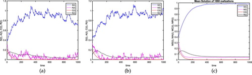
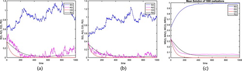
Figure 2. The plot shows the extinction of the proposed model $\left(1\right)$ for $\sigma =0.35$. Comparing with Figure (1), with the noise getting smaller, the fluctuation of the solution of system (1(1) $\begin{array}{rl}\mathrm{d}S\left(t\right)& =(b-\alpha S\left(t\right)C\left(t\right)-(v+{\mu }_0)S\left(t\right))\mathrm{d}t-\sigma S\left(t\right)C\left(t\right)\mathrm{d}B\left(t\right),\\ \mathrm{d}A\left(t\right)& =(\alpha S\left(t\right)C\left(t\right)-({\gamma }_1+{\mu }_0+\text{β})A\left(t\right))\mathrm{d}t+\sigma S\left(t\right)C\left(t\right)\mathrm{d}B\left(t\right),\\ \mathrm{d}C\left(t\right)& =(\text{β}A\left(t\right)-({\gamma }_2+{\mu }_0+{\mu }_1)C\left(t\right))\mathrm{d}t,\\ \mathrm{d}R\left(t\right)& =vS\left(t\right)+({\gamma }_{2}C\left(t\right)-{\mu }_{0}R\left(t\right)+{\gamma }_{1}A\left(t\right))\mathrm{d}t.\end{array}$(1) ) is getting weaker. (a) Test 2: Realization 1 with time in days. (b) Test 2: Realization 2 with time in days. (c) Test 2: Mean Solution with time in days.

We examine two tests, using the parameters and initial data as mentioned in Table 2:

Table 2. List of parameters.

	Test 1	Test 2
$C_0$	1.3	1.3
$R_0$	0.5	0.5
$A_0$	0.8	0.8
$S_0$	0.3	0.3
$C_s$	1.3461	1.3461
$R_s$	0.5121	0.5121
$A_s$	0.1513	0.1513
$S_s$	0.9246	0.9246
${\mu }_1$	0.2	0.2
${\mu }_0$	0.5	0.5
${\gamma }_1$	0.2	0.4
${\gamma }_2$	0.4	0.2
b	0.5	0.5
α	0.60	0.360
v	0.01	0.01
β	0.1	0.4
σ	0.5	0.35

Remark that the results of the two tests show the stability of the system (1). Moreover, we have for our Tests: $\begin{array}{rl}\mathrm{T}\mathrm{e}\mathrm{s}\mathrm{t}1& =C_T\le A_T\le R_T\le S_T,\\ \mathrm{T}\mathrm{e}\mathrm{s}\mathrm{t}2& =C_T\le R_T\le A_T\le S_T.\end{array}$

6. Conclusion

Most of the real-world problems include stochastic influence. In the current paper, we investigated the transmission dynamics of the HBV stochastic epidemic model. By using a proper stochastic Lyapunov function, we showed the existence of positive solutions. We obtained sufficient conditions for the extinction and persistence of the hepatitis B in terms of the parameters involved in the model. We also proved that the intensity of the noise has a significant influence on the transmission of the disease. We showed that the extinction of the disease increases with the increase in the noise parameter. Similarly, the disease decreases with the increased noise term. All these theoretical findings are verified using Itô-Taylor stochastic scheme (also called the Milstein scheme).

Remark Tahir Khan et al. [10] have studied system (1), comparing with Theorem 5.1, our conditions for extinction are much more simple. Also the basic reproductive number $R_0$ presented in Equation (23) of [10] is very cumbersome as compare to our $R_0$ in (17). Moreover, we see that if $\sigma =0$, the condition is reduced to $R_0>1$, which is the condition for globally asymptotically stable of endemic equilibrium $P^{\ast }$ of system (2). And $R_0$ is smaller than the basic reproduction number $R_0^d$ of system (2). Hence, we can make a conjecture that the behaviour of the disease is determined by $R_0$. It is well known that for deterministic epidemic models, the basic reproduction number determines the prevalence or extinction of the disease. Notice that $R_0<R_0^d$, and it is possible that $R_0<1<R_0^d$. This is the case when the deterministic model has an endemic.

Disclosure statement

No potential conflict of interest was reported by the author(s).

References

- L.J.S. Allen, An introduction to stochastic epidemic models, in Mathematical Epidemiology, F. Brauer, P. van den Driessche, J. Wu, eds., Springer, Berlin, Heidelberg, 2008, pp. 81–130
- J.R. Beddington and R.M. May, Harvesting natural populations in a randomly fluctuating environment, Science 197 (1977), pp. 463–465. doi: 10.1126/science.197.4302.463
- T. Britton and D. Lindenstrand, Epidemic modelling: aspects where stochastic epidemic models: a survey, Math. Biosci. 222 (2010), pp. 109–116. doi: 10.1016/j.mbs.2009.10.001
- Y. Cai, Y. Kang, M. Banerjee, and W. Wang, A stochastic epidemic model incorporating media coverage, Commun. Math. Sci. 14 (2016), pp. 892–910. doi: 10.4310/CMS.2016.v14.n4.a1
- N. Dalal, D. Greenhalgh, and X. Mao, A stochastic model for internal HIV dynamics, J. Math. Anal. Appl. 341 (2008), pp. 1084–1101. doi: 10.1016/j.jmaa.2007.11.005
- W.J. Edmunds, G.F. Medley, and D.J. Nokes, The transmission dynamics and control of hepatitis B virus in the Gambia, Stat. Medic 15 (1996), pp. 2215–2233. doi: 10.1002/(SICI)1097-0258(19961030)15:20<2215::AID-SIM369>3.0.CO;2-2
- A. Gray, D. Greenhalgh, L. Hu, X. Mao, and J. Pan, A stochastic differential equation SIS epidemic model, SIAM J. Appl. Math. 71 (2011), pp. 876–902. doi: 10.1137/10081856X
- Q. Han, L. Chen, and D. Jiang, A note on the stationary distribution of stochastic SEIR epidemic model with saturated incidence rate, Sci. Rep. 7(1) (2017), p. 3996. doi: 10.1038/s41598-017-03858-8
- C. Ji and D. Jiang, Threshold behaviour of a stochastic SIR model, Appl. Math. Model. 38 (2014), pp. 5067–5079. doi: 10.1016/j.apm.2014.03.037
- T. Khan, I.H. Jung, and G. Zaman, A stochastic model for the transmission dynamics of hepatitis B virus, J. Biol. Dyn. 13(1) (2019), pp. 328–344. doi: 10.1080/17513758.2019.1600750
- T. Khan, A. Khan, and G. Zaman, The extinction and persisitence of the stochastic hepatitis B epidemic model, Chaos. Sol. Fractals 108 (2018), pp. 123–128. doi: 10.1016/j.chaos.2018.01.036
- T. Khan and G. Zaman, Classification of different hepatitis B infected individuals with saturated incidence rate, SpringerPlus. 5 (2016), pp. 1082. doi: 10.1186/s40064-016-2706-3
- T. Khan, G. Zaman, and M.I. Chohan, The transmission dynamic and optimal control of acute and chronic hepatitis B, J. Biol. Dyn. 11 (2017), pp. 172–189. doi: 10.1080/17513758.2016.1256441
- A. Lahrouz and L. Omari, Extinction and stationary distribution of a stochastic SIRS epidemic model with non-linear incidence, Stat. Prob. Lett. 83 (2013), pp. 960–968. doi: 10.1016/j.spl.2012.12.021
- Q. Lu, Stability of SIRS system with random perturbations, Phys. A Stat. Mech. Appl. 388 (2009), pp. 3677–3686. doi: 10.1016/j.physa.2009.05.036
- J. Mann and M. Roberts, Modelling the epidemiology of hepatitis B in New Zealand, J. Theor. Biol. 269 (2011), pp. 266–272. doi: 10.1016/j.jtbi.2010.10.028
- A. Mwasa and J.M. Tchuenche, Mathematical analysis of a cholera model with public health interventions, Biosystems 105 (2011), pp. 190–200. doi: 10.1016/j.biosystems.2011.04.001
- B. Øksendal, Stochastic Differential Equations, Springer, Berlin, Heidelberg, 2003.
- J. Pang, J.A. Cui, and X. Zhou, Dynamical behavior of a hepatitis B virus transmission model with vaccination, J. Theor. Biol. 265 (2010), pp. 572–578. doi: 10.1016/j.jtbi.2010.05.038
- S. Thornley, C. Bullen, and M. Roberts, Hepatitis B in a high prevalence New Zealand population: a mathematical model applied to infection control policy, J. Theor. Biol. 254 (2008), pp. 599–603 doi: 10.1016/j.jtbi.2008.06.022
- J.E. Truscott and C.A. Gilligan, Response of a deterministic epidemiological system to a stochastically varying environment, Proc. Nat. Acad. Sci. 100 (2003), pp. 9067–9072. doi: 10.1073/pnas.1436273100
- F. Wei and C. Fangxiang, Stochastic permanence of an SIQS epidemic model with saturated incidence and independent random perturbations, Phys. A Stat. Mech. Appl. 453 (2016), pp. 99–107. doi: 10.1016/j.physa.2016.01.059
- M. Zahri, Multidimensional Milstein scheme for solving a stochastic model for prebiotic evolution, Jou. Tai. Uni. Sci. 8(2) (2014), pp. 186–198. doi: 10.1016/j.jtusci.2013.12.002
- M. Zahri, Barycentric interpolation of interface-solution for solving SPDEs on non-overlapping subdomains with additive multi-noises, Inter. J. Comp. Math. 95(4) (2018), pp. 645–685. doi: 10.1080/00207160.2017.1297429
- G. Zaman, Y.H. Kang, and I.H. Jung, Stability analysis and optimal vaccination of an SIR epidemic model, BioSystems 93(3) (2008), pp. 240–249. doi: 10.1016/j.biosystems.2008.05.004
- T. Zhang, K. Wang, and X. Zhang, Modeling and analyzing the transmission dynamics of HBV epidemic in Xinjiang, China, PLoS One 10 (2015), p. e0138765. doi: 10.1371/journal.pone.0138765
- Y. Zhao, D. Jiang, and D. O'Regan, The extinction and persistence of the stochastic SIS epidemic model with vaccination, Phys. A Stat. Mech. Appl. 392 (2013), pp. 4916–4927. doi: 10.1016/j.physa.2013.06.009
- S. Zhao, Z. Xu, and Y. Lu, A mathematical model of hepatitis B virus transmission and its application for vaccination strategy in China, Int. J. Epidemiol. 29 (2000), pp. 744–752. doi: 10.1093/ije/29.4.744
- Y. Zhao, Q. Zhang, and D. Jiang, The asymptotic behavior of a stochastic SIS epidemic model with vaccination, Adv. Diff. Equ. 2015(1) (2015), pp. 328. doi: 10.1186/s13662-015-0592-6
- Y. Zhou, W. Zhang, and S. Yuan, Survival and stationary distribution of a SIR epidemic model with stochastic perturbations, Appl. Math. Comput. 244 (2014), pp. 118–131.
- L. Zou, W. Zhang, and S. Ruan, Modeling the transmission dynamics and control of hepatitis B virus in China, J. Theor. Biol. 262 (20100), pp. 330–338. doi: 10.1016/j.jtbi.2009.09.035
- L. Zou, W. Zhang, and S. Ruan, Modeling the transmission dynamics and control of hepatitis B virus in China, J. Theor. Biol. 262 (2010), pp. 330–338. doi: 10.1016/j.jtbi.2009.09.035