Modelling the risk of HIV infection for drug abusers

ABSTRACT

Drugs of abuse, such as opiates, are one of the leading causes for transmission of HIV in many parts of the world. Drug abusers often face a higher risk of acquiring HIV because target cell (CD4+ T-cell) receptor expression differs in response to morphine, a metabolite of common opiates. In this study, we use a viral dynamics model that incorporates the T-cell expression difference to formulate the probability of infection among drug abusers. We quantify how the risk of infection is exacerbated in morphine conditioning, depending on the timings of morphine intake and virus exposure. With in-depth understanding of the viral dynamics and the increased risk for these individuals, we further evaluate how preventive therapies, including pre- and post-exposure prophylaxis, affect the infection risk in drug abusers. These results are useful to devise ideal treatment protocols to combat the several obstacles those under drugs of abuse face.

Keywords:

• Drugs of abuse
• human immunodeficiency virus
• mathematical models
• prophylaxis
• risk of infection

2010 Mathematics Subject Classifications:

• 34D20
• 37N25
• 92B05
• 92C50

1. Introduction

The human immunodeficiency virus (HIV) remains a persistent epidemic in the USA and worldwide. It has been commonly understood that drugs of abuse, such as opiates, are one of the leading causes of HIV transmission. According to the World Health Organization [45], out of the 13 million people who inject drugs worldwide, 1.7 million of them are living with HIV. More specifically, injection drug use accounts for nearly a third of all HIV infections in the USA [4,10,25]. Given the high risk of infection associated with drugs of abuse, it is of paramount importance to study HIV dynamics and the risk of infection in the context of drugs of abuse.

Opioids remain a major class of commonly abused drugs, among which heroin is one of the most common in the drug abuser community [6]. Since a metabolite of heroin is morphine [22], morphine is a common opiate used for experimental studies related to drugs of abuse. Drugs of abuse are typically attributed to a higher risk of HIV infection due to needle sharing and increased risky sexual behaviour [9,29]. While these behavioural factors contribute to an increased risk of transmission, an alteration of biological components due to conditioning of drugs of abuse has been shown to have a significant impact on the risk of infection. Several experiments utilizing simian immunodeficiency virus (SIV) infection in macaques have shown that when morphine is present within a body, the population dynamics of CD4 T cells, which are the primary target of HIV, change [16,17]. In particular, morphine promotes co-receptor expression in CD4 T cells, and these co-receptors, such as CCR5 and CXCR4, are utilized by HIV to establish infection in CD4 T cells [27,40]. An increase of co-receptor expression due to the presence of morphine increases the susceptibility of target cells (CD4 T cells) to HIV infection. As a consequence, the risk of infection may change as a result of the presence of morphine in the body of virus recipients. It is of utmost importance to properly quantify the risk of infection in order to devise an ideal strategy for HIV prevention among drug abusers. One of the main objectives of this study is to predict the risk of HIV infection when morphine is present within a body and to identify how much the risk of infection can be reduced by using preventive therapies.

Mathematical models have been a powerful tool to describe HIV dynamics within hosts. In this study, we implement a recently developed mathematical model under conditioning of drugs of abuse to predict the risk of HIV transmission from infected individuals to uninfected drug abusers. Our novel probabilistic model takes into account three vital steps for a successful infection: virus transfer from a source partner to the target cell site within a drug abuser, initial infection of a target cell, and persistence of infection within the drug abuser host. Using our model, we quantify the risk of infection in morphine conditioning depending on the timings of morphine intake and virus exposure. Our model predicts that the presence of morphine can set a condition with significant increase in the risk of HIV infection, underscoring a need of proper evaluation of prevention strategy for drug abusers.

In a current situation of unavailability of an effective HIV vaccine, treatment as prevention has been considered as planning for curbing the HIV epidemic. In particular, individuals in risky groups, such as injection drug users and sexual workers, are recommended to use pre- and/or post-exposure prophylaxis (PrEP/ PEP) as a way to prevent the virus transmission [21]. We extended our basic probabilistic model for drug abusers to incorporate preventive therapy and used the extended model to evaluate the role of pre- and post-exposure prophylaxis in reducing the risk of HIV infection. Importantly, our results indicate that the effectiveness of therapy on reducing the risk of HIV infection highly depends on the timing of therapy initiation.

2. Cell population switch under morphine conditioning

To quantify the risk of HIV infection, it is necessary to understand target cell (CD4 T cell) dynamics, which is affected by morphine conditioning. In this section, we analyse a mathematical model that describes T-cell dynamics under morphine conditioning in the absence of virus. When an opiate interacts with target cells, it affects the co-receptors by increasing their expression. Morphine has been proven to modulate co-receptor expression of CD4 T cells, specifically the expressions of CCR5 and CXCR4 co-receptors [12,19,39]. An increase in the co-receptor expression in a target cell causes the cell to be more susceptible to HIV infection as the virus fusion into the cell is mediated through the help of these co-receptors.

As mentioned earlier, our objective is to compute the risk of infection in uninfected drug abusers. Since the infection has not been established in these individuals, HIV-specific immune responses are absent. Therefore, other immune cells, such as CD8 T cells and B cells, are ignored, and only CD4 T cells, the primary target of HIV, are considered in our model. To describe the effect of morphine on switching CD4 T cells between different susceptibilities, we consider two subpopulations of these cells as done previously [44]: a low susceptibility category, $T_l$, and a high susceptibility category, $T_h$. We describe the dynamics of these cells using the following model equations. 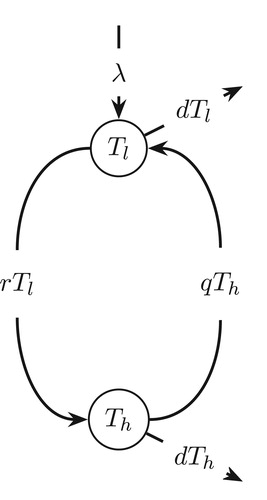(1) $\begin{array}{rl}\dot{T_l}& =\lambda -\mathrm{d}{T}_l-r{T}_l+q{T}_h,T_l(0)=T_{l0},\\ \dot{T_h}& =r{T}_l-\mathrm{d}{T}_h-q{T}_h,T_h(0)=T_{h0}.\end{array}$(1) In this model, target cells are assumed to be generated in the low susceptible category, $T_l$, at a rate of λ cells per day. Cells transit from the low, $T_l$, to high, $T_h$, susceptible category at rate r, and from high to low at rate q. These target cells die at per capita death rate of d per day. A schematic diagram of the cell population switch model is shown in Figure 1.

Figure 1. Schematic diagram of target cell population switch model.

In the absence of HIV infection, the total amount of CD4 T cells in uninfected individuals remains approximately constant, i.e.$T_l+T_h=T_{l0}+T_{h0}=T_0$, a constant. This implies that $\dot{T_l}+\dot{T_h}=0$, which from Model 1(1) $\begin{array}{rl}\dot{T_l}& =\lambda -\mathrm{d}{T}_l-r{T}_l+q{T}_h,T_l(0)=T_{l0},\\ \dot{T_h}& =r{T}_l-\mathrm{d}{T}_h-q{T}_h,T_h(0)=T_{h0}.\end{array}$(1) , gives $\lambda =d(T_l+T_h)=\mathrm{d}{T}_0$. Then, solving the differential equations, we obtain (2a) $\begin{array}{rl}{T}_h(t)& =\frac{r{T}_0+[(d+q+r)T_{h0}-r{T}_0]e^{-(d+q+r)t}}{d+q+r},\end{array}$(2a) (2b) $\begin{array}{rl}{T}_l(t)& =T_0-T_h(t).\end{array}$(2b)

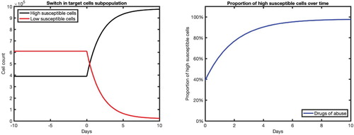
Since morphine causes a cell population switch, the model parameters that are affected by morphine are r and q. For example, an estimation using the data from morphine addicted SIV-infected macaques [44] shows a higher r and a lower q in the presence of morphine (r = 0.5 per day, $q=4.42\times {10}^{-7}$ per day in the presence of morphine and r = 0.16 per day, q = 0.24 per day in the absence of morphine).

In Figure 2, we present the typical cell dynamics predicted by Equations (2a(2a) $\begin{array}{rl}{T}_h(t)& =\frac{r{T}_0+[(d+q+r)T_{h0}-r{T}_0]e^{-(d+q+r)t}}{d+q+r},\end{array}$(2a) ) and (2b(2b) $\begin{array}{rl}{T}_l(t)& =T_0-T_h(t).\end{array}$(2b) ), within a susceptible individual under morphine conditioning. In this case, morphine enters the system at day 0, before which the cell subpopulation is assumed to be at the steady state (a constant level before morphine intake). The proportion of high susceptible cells, $P=\frac{T_h}{T_l+T_h}$, rapidly increases after morphine exposure (Figure 2 right). In the absence of morphine, the proportion of high susceptible cells remains at approximately 39% while with a prolonged maintenance of morphine, this proportion reaches approximately 98% within 10 days. This implies that the maintenance of a constant level of morphine can cause the proportion of high susceptible cells to be more than double in the body of drug abusers. Depending on when the virus is introduced, before or after the morphine intake, the number of high susceptible cells available can be quite different. The dynamical nature of the high susceptible cells post-morphine intake indicates that the risk of infection may depend on the amount of time between morphine intake and virus exposure.

Figure 2. Dynamics of cell subpopulations (left) and proportion of high susceptible cells (right) in the absence of virus infection. Time t = 0 represents the time of morphine intake. Before the morphine intake ($t\le 0$), the cell populations are assumed to be at the steady state $T_l=T_0(d+q)/(d+q+r)\sim 6.1\times {10}^5,T_h=T_{0}r/(d+q+r)\sim 3.9\times {10}^5$ (with parameters corresponding to the absence of morphine, i.e. $T_0={10}^6,d=0.01,r=0.16,q=0.24$). After the morphine intake ($t\ge 0$), the parameters corresponding to the presence of morphine are used (i.e. $d=0.01,r=0.5,q=4.42\times {10}^{-7},T_{l0}=6.1\times {10}^5,T_{h0}=3.9\times {10}^5$).

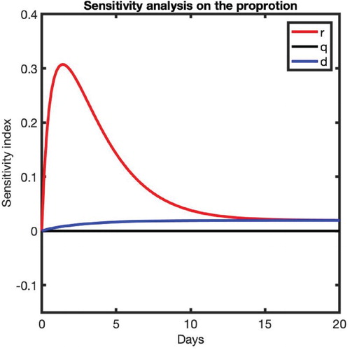
We also performed a sensitivity analysis to identify the most impactful parameter on the proportion of high susceptible cells, P, by computing the following sensitivity index $S_x=\frac{x}{P}\frac{\mathrm{\partial }P}{\mathrm{\partial }x},$where x is a parameter, whose impact on P is sought [30]. Note that the higher the value of $S_x$, the more impactful the parameter is. Also, a positive (negative) value indicates that an increase in the parameter increases (decreases) P. Our computations (Figure 3) reveal that the most impactful parameter on the proportion of high susceptible cells is r, the rate at which low susceptible cells, $T_l$, transit to the high susceptible category, $T_h$. The impact is particularly pronounced at the beginning of the morphine intake until about 10 days post-morphine intake. A higher positive effect of r indicates that the presence of a higher amount of morphine results in a higher proportion of high susceptible cells. The parameters q and d have low sensitivity indices, implying that they have a low effect on the proportion of high susceptible cells, P.

Figure 3. Sensitivity analysis of parameters on the proportion of high susceptible cells, P. The value on the y-axis represents the sensitivity index, $S_x$ and the time t = 0 represents the time of morphine intake.

3. Formulation of risk of infection

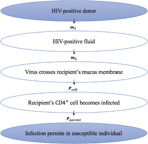
We define a risk of infection, $P_{\inf }$, as the probability of a successful establishment of HIV infection in a susceptible individual upon a single contact (exposure to virus source) with an HIV-infected individual. In order for a susceptible individual (recipient) to become infected upon contact with an infected individual (donor), three steps must occur:

1. transmission (the transfer of virus from the donor to the site of the target cells of the recipient)

2. infection initiation (infection of at least one target cell by the virus)

3. infection persistence (establishment of a persistent infection by infecting other cells)

A detailed stepwise process starting from virus in the donor to a successful establishment of HIV infection in the recipient is depicted through a schematic diagram in Figure 4. We now formulate each step leading to an overall risk of infection, $P_{\inf }$, which is a combined effect of the transfer of virus from the donor to the recipient, the probability of infection initiation, $P_{\mathrm{cell}}$, and the probability of infection persistence, $P_{\mathrm{persist}}.$

Figure 4. Schematic diagram showing steps starting from virus in the donor to a successful establishment of HIV infection in the recipient.

Step-1: Transmission

We denote a viral load in the blood of the donor as $V_{\mathrm{donor}}$ per mL, which can be clinically measured in HIV-infected patients. We take $m_1$ to represent the ratio between the viral concentration in the blood and the released bodily fluid, such as semen, of the donor such that the recipient is exposed to the total $m_1{V}_{\mathrm{donor}}$ viruses. We further assume that a fraction $m_2$ of these exposed viruses cross any mucus barrier and reach the target cell site of the recipient [24]. Thus, the total amount of viruses that survive transmission and make it to the recipient's target cell site is given by $m{V}_{\mathrm{donor}}$, where $m=m_1{m}_2$. Depending on the mode of transmission, m can take on several different values. For example, the value of m is higher when the mode of transmission is injection drug use rather than sexual contact, as the virus is directly injected into the blood causing fewer barriers to cross to make it to the target cell site [42].

Step-2: Infection initiation

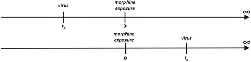
In this section, we formulate the probability, $P_{\mathrm{cell}}$, that the viruses that reached the recipient's target cell site infect at least one of the target cells. We consider the time of the morphine intake as t = 0 (same as above) and the time of virus exposure as $t=t_p$ (Figure 5). A positive $t_p$ represents virus being introduced after morphine has entered the system and a negative $t_p$ represents virus being introduced before morphine intake (Figure 5).

Figure 5. Timeline showing the time of morphine intake (t = 0) and the time of virus exposure ($t=t_p$). When the recipient is exposed to virus before morphine intake (top, $t_p<0$) and after morphine intake (bottom, $t_p>0$).

In the absence of target cell infection, free virus, V, gets cleared by the body at a virus clearance rate c. The dynamics of virus introduced into the target cell site at the time of virus exposure $t=t_p$ is governed by the equation (3) $\dot{V}=-cV,V(t_p)=m{V}_{\mathrm{donor}}.$(3) By solving Equation 3(3) $\dot{V}=-cV,V(t_p)=m{V}_{\mathrm{donor}}.$(3) , we find $V(s)=m{V}_{\mathrm{donor}}{e}^{-c(s-t_p)},s\ge t_p$, which provides the amount of virus that survive at the end of the time interval of $[t_p,t_i]$ to be $V(t_i)$ [23]. We assume the infection rate of low ($T_l$) and high ($T_h$) susceptible cells to be ${\beta }_l$ per virus per day and ${\beta }_h$ per virus per day, respectively. Thus, the total cell infection rate per virus is given by $({\beta }_l{T}_l+{\beta }_h{T}_h)$ per day.

As in previous work [1,31,42], we now assume that the viral infection of target cells follows an inhomogeneous Poisson process. Here, the Poisson parameter represents the expected number of newly infected target cells of the recipient in the time interval $[t_p,t_i]$, which is given by (4) $\gamma (t_i)=m{V}_{\mathrm{donor}}{\int }_{t_p}^{t_i}{e}^{-c(s-t_p)}[{\beta }_l{T}_l(s)+{\beta }_h{T}_h(s)]\mathrm{d}s.$(4) Then using the Poisson process [1,31,42], we obtain the probability that at least one target cell becomes ultimately infected as $\underset{t_i\to \mathrm{\infty }}{lim}(1-e^{-\gamma (t_i)})$. Hence, the probability of infection initiation is given by (5) $P_{\mathrm{cell}}=1-\exp (-m{V}_{\mathrm{donor}}{\int }_{t_p}^{\mathrm{\infty }}{e}^{-c(s-t_p)}[{\beta }_l{T}_l(s)+{\beta }_h{T}_h(s)]\mathrm{d}s),$(5) where the dynamics of $T_h$ and $T_l$ before morphine intake (t<0) and after morphine intake (t>0), as discussed in Section 2, are given by (6a) $\begin{array}{rl}{T}_h(t)& =\{\begin{array}{ll}{T}_{h0}& \mathrm{if}t<0,\\ {\displaystyle \frac{r{T}_0+[(d+q+r)T_{h0}-r{T}_0]e^{-(d+q+r)t}}{d+q+r}}& \mathrm{if}t\ge 0,\end{array}\end{array}$(6a) (6b) $\begin{array}{rl}{T}_l(t)& =T_0-T_h(t).\end{array}$(6b)

Step-3: Infection persistence

We assume that a single cell is successfully infected at time $t=t_i\ge t_p$, where $t_p$ is the time of virus exposure as discussed above. Given the single cell is successfully infected, we now formulate the probability that the initiated infection establishes a persistent infection, $P_{\mathrm{persist}}$. For this, we again assume the inhomogeneous Poisson process, with a new Poisson parameter. This new parameter represents the expected number of secondary infections from a single infected cell, which is known as the basic reproduction number, $R_0$ [3]. For $t\ge t_i$ (after infection initiation), we extend Model (1(1) $\begin{array}{rl}\dot{T_l}& =\lambda -\mathrm{d}{T}_l-r{T}_l+q{T}_h,T_l(0)=T_{l0},\\ \dot{T_h}& =r{T}_l-\mathrm{d}{T}_h-q{T}_h,T_h(0)=T_{h0}.\end{array}$(1) ) to incorporate the dynamics of infected cells, I, and free virus, V, along with target cells, $T_l$ and $T_h$. The governing equations are as follows. (7) $\begin{array}{rl}\dot{T_l}& =\lambda -\mathrm{d}{T}_l-r{T}_l-{\beta }_l{T}_{l}V+q{T}_h,\\ \dot{T_h}& =r{T}_l-\mathrm{d}{T}_h-{\beta }_h{T}_{h}V-q{T}_h,\\ \dot{I}& ={\beta }_l{T}_{l}V+{\beta }_h{T}_{h}V-\delta I,\\ \dot{V}& =pI-cV,\end{array}$(7) with initial conditions at the time of infection initiation, $T_l(t_i)$, $T_h(t_i)$, $I(t_i)=1$, and $V(t_i)$. The schematic diagram of the model is shown in Figure 6. Target cells, $T_l$ and $T_h$ become infected cells, I, when they come in contact with free virus, V, at rates ${\beta }_l$ and ${\beta }_h$, respectively. δ represents the death rate of infected cells, and p and c are rate constants for virus production per infected cell and virus clearance, respectively. A comprehensive list of the parameters, their meanings, and values are shown in Table 1 [44].

Figure 6. Schematic diagram of viral dynamics after infection is initiated.

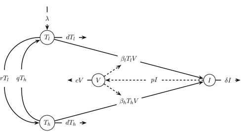
Table 1. Model parameters.

	Meaning	Value	Units	Source
δ	Death rate of infected cells	0.38	day${}^{-1}$	[44]
d	Death rate of uninfected cells	0.01	day${}^{-1}$	[38]
λ	Target cell production rate	${10}^4$	cell ml${}^{-1}$ day${}^{-1}$	[38]
r	Rate of switch $T_l$ to $T_h$	0.5 (morphine)	day${}^{-1}$	[44]
		0.16 (no morphine)
q	Rate of switch $T_h$ to $T_l$	$4.42\times {10}^{-7}$ (morphine)	day${}^{-1}$	[44]
		0.24 (no morphine)
${\beta }_l$	Infection rate of $T_l$	5.13$\times {10}^{-10}$	ml day${}^{-1}$virion${}^{-1}$	[44]
${\beta }_h$	Infection rate of $T_h$	3.02$\times {10}^{-8}$	ml day${}^{-1}$virion${}^{-1}$	[44]
p	Virus production rate	2500	virion day${}^{-1}$cell${}^{-1}$	[44]
c	Clearance rate of virus	23	day${}^{-1}$	[26]
m	Fraction of viruses reaching target cells	$1.64\times {10}^{-5}$	dimensionless	[46], Estimated

To compute the basic reproduction number, $R_0$ (the Poisson parameter for $P_{\mathrm{persist}}$), we use the next generation matrix method [18,48] on Model (7(7) $\begin{array}{rl}\dot{T_l}& =\lambda -\mathrm{d}{T}_l-r{T}_l-{\beta }_l{T}_{l}V+q{T}_h,\\ \dot{T_h}& =r{T}_l-\mathrm{d}{T}_h-{\beta }_h{T}_{h}V-q{T}_h,\\ \dot{I}& ={\beta }_l{T}_{l}V+{\beta }_h{T}_{h}V-\delta I,\\ \dot{V}& =pI-cV,\end{array}$(7) ). According to the next generation method, we compute the Jacobian, J, of the infectious equations, ($\dot{I},\dot{V}$), linearized about the infection-free equilibrium, $\mathrm{IFE}=(\frac{\lambda (d+q)}{d(d+q+r)},\frac{\lambda r}{d(d+q+r)},0,0)$. The Jacobian is then split into two matrices, F (the new infection matrix) and V (the transfer matrix) such that J = F−V, $\mathbf{F}=\left[\begin{array}{cc}0& {\beta }_l\left({\displaystyle \frac{\lambda (d+q)}{d(d+q+r)}}\right)+{\beta }_h\left({\displaystyle \frac{\lambda r}{d(d+q+r)}}\right)\\ p& 0\end{array}\right],\mathbf{V}=\left[\begin{array}{cc}\delta & 0\\ 0& c\end{array}\right].$The spectral radius of $\mathbf{F}{\mathbf{V}}^{-1}$ gives the basic reproduction number, i.e. $R_0=\rho (\mathbf{F}{\mathbf{V}}^{-1})$. Hence, (8) $R_0=\frac{\lambda p[{\beta }_l(d+q)+{\beta }_{h}r]}{\delta cd(d+r+q)}.$(8) Note that the basic reproduction number can take on different values depending on the availability of the two different target cell subpopulations ($T_l(t_i),T_h(t_i)$) (Figure 2) at the time of infection initiation. Since the lifespan of free virus particles and infected cells is short, the difference between target cell populations at $t_i$ (the time of infection initiation) and at $t_p$ (the time of virus exposure) can be assumed to be negligible, implying ($T_l(t_i),T_h(t_i)$) ∼ ($T_l(t_p),T_h(t_p)$). Thus, replacing the expression of $\mathrm{IFE}=(\frac{\lambda (d+q)}{d(d+q+r)},\frac{\lambda r}{d(d+q+r)},0,0)$ in Equation (8(8) $R_0=\frac{\lambda p[{\beta }_l(d+q)+{\beta }_{h}r]}{\delta cd(d+r+q)}.$(8) ) by the initial infection-free condition $(T_l(t_p),T_h(t_p),0,0)$, we obtain the basic reproduction number as (9) $R_0=\frac{p}{c\delta }[{\beta }_l{T}_l(t_p)+{\beta }_h{T}_h(t_p)],$(9) where (10a) $\begin{array}{rl}{T}_h(t_p)& =\{\begin{array}{ll}{T}_{h0}& \mathrm{if}{t}_p<0,\\ {\displaystyle \frac{r{T}_0+[(d+q+r)T_{h0}-r{T}_0]e^{-(d+q+r)t_p}}{d+q+r}}& \mathrm{if}{t}_p\ge 0,\end{array}\end{array}$(10a) (10b) $\begin{array}{rl}{T}_l(t_p)& =T_0-T_h(t_p).\end{array}$(10b)

As established in the following three theorems, we are able to prove that $R_0$ can fully describe both virus and cell dynamics after the initiation of infection.

Theorem 3.1

If $R_0<1$, the infection-free equilibrium is locally asymptotically stable and if $R_0>1$ the IFE is unstable.

Proof.

See Appendix 1.

Theorem 3.2

If $R_0<1$, the infection-free equilibrium is globally asymptotically stable.

Proof.

See Appendix 2.

Theorem 3.3

If $R_0>1$, system (7(7) $\begin{array}{rl}\dot{T_l}& =\lambda -\mathrm{d}{T}_l-r{T}_l-{\beta }_l{T}_{l}V+q{T}_h,\\ \dot{T_h}& =r{T}_l-\mathrm{d}{T}_h-{\beta }_h{T}_{h}V-q{T}_h,\\ \dot{I}& ={\beta }_l{T}_{l}V+{\beta }_h{T}_{h}V-\delta I,\\ \dot{V}& =pI-cV,\end{array}$(7) ) is uniformly persistent with respect to $({\mathbb{X}}_0,\mathrm{\partial }{\mathbb{X}}_0)$, where $\mathbb{X}={\mathbb{R}}_{+}^4$, such that there exists a positive constant $\xi >0$, and every solution $(T_l(t),T_h(t),I(t),V(t))$ with initial value $(T_{l0},T_{h0},I_0,V_0)\in {\mathbb{X}}_0$ satisfies (11) $\underset{t\to \mathrm{\infty }}{lim}infI(t)\ge \xi ,\underset{t\to \mathrm{\infty }}{lim}infV(t)\ge \xi .$(11) Furthermore, system (7(7) $\begin{array}{rl}\dot{T_l}& =\lambda -\mathrm{d}{T}_l-r{T}_l-{\beta }_l{T}_{l}V+q{T}_h,\\ \dot{T_h}& =r{T}_l-\mathrm{d}{T}_h-{\beta }_h{T}_{h}V-q{T}_h,\\ \dot{I}& ={\beta }_l{T}_{l}V+{\beta }_h{T}_{h}V-\delta I,\\ \dot{V}& =pI-cV,\end{array}$(7) ) admits at least one positive equilibrium.

Proof.

See Appendix 3.

These three theorems have important biological interpretations. Note that $R_0$ represents the average number of infected cells produced by a single infected cell and can be estimated using the model parameters (Equations (8(8) $R_0=\frac{\lambda p[{\beta }_l(d+q)+{\beta }_{h}r]}{\delta cd(d+r+q)}.$(8) ) and (9(9) $R_0=\frac{p}{c\delta }[{\beta }_l{T}_l(t_p)+{\beta }_h{T}_h(t_p)],$(9) )). According to the Theorems 3.1 and 3.2, if the magnitude of $R_0$ is less than unity, the infection dies out eventually converging to the infection-free equilibrium. On the other hand, the Theorem 3.3 shows that if the magnitude of $R_0$ is greater than unity, the infection establishes with virus persisting in the body.

While $R_0>1$ can ascertain the persistence of infection in the deterministic dynamics (Theorem 3.3), due to the small number of initially infected cells, the infection may not persist because of the stochastic nature of cell dynamics [8,15]. To incorporate this stochastic factor, we use $R_0$ as a rate parameter in the Poisson process, which implies the probability of infection persistence is ($1-e^{-R_0}$). Therefore, the probability, $P_{\mathrm{persist}}$, that the initiated infection establishes a persistent infection is given by (12) $P_{\mathrm{persist}}=1-\exp (-\frac{p[{\beta }_l{T}_l(t_p)+{\beta }_h{T}_h(t_p)]}{c\delta }),$(12) where (13a) $\begin{array}{rl}{T}_h(t_p)& =\{\begin{array}{ll}{T}_{h0}& \mathrm{if}{t}_p<0,\\ {\displaystyle \frac{r{T}_0+[(d+q+r)T_{h0}-r{T}_0]e^{-(d+q+r)t_p}}{d+q+r}}& \mathrm{if}{t}_p\ge 0,\end{array}\end{array}$(13a) (13b) $\begin{array}{rl}{T}_l(t_p)& =T_0-T_h(t_p).\end{array}$(13b)

Overall risk of infection

We now combine all steps to formulate the overall risk of infection. The probability of a susceptible individual becoming infected from a single contact with an infected individual having a viral load of $V_{\mathrm{donor}}$ is given by (14) $\begin{array}{rl}{P}_{\inf }& =P_{\mathrm{cell}}\cdot P_{\mathrm{persist}}\\ & =[1-e^{-m{V}_{\mathrm{donor}}{\int }_{t_p}^{\mathrm{\infty }}{e}^{-c(s-t_p)}({\beta }_l{T}_l(s)+{\beta }_h{T}_h(s))\mathrm{d}s}][1-e^{-\frac{p[{\beta }_l{T}_l(t_p)+{\beta }_h{T}_h(t_p)]}{c\delta }}],\end{array}$(14) where (15a) $\begin{array}{rl}{T}_h(t)& =\{\begin{array}{ll}{T}_{h0}& \mathrm{if}t<0,\\ {\displaystyle \frac{r{T}_0+[(d+q+r)T_{h0}-r{T}_0]e^{-(d+q+r)t}}{d+q+r}}& \mathrm{if}t\ge 0,\end{array}\end{array}$(15a) (15b) $\begin{array}{rl}{T}_l(t)& =T_0-T_h(t).\end{array}$(15b)

4. Computation of risk of infection

Model parameters are estimated based on literature survey [26,38,43,44] and are given in Table 1. Note that as discussed above, the transmission-related parameter, m, depends upon the mode of transmission. For sexual transmission, the risk of receiving HIV from an infected individual has been estimated to be 0.82% per coital act [46]. Thus, we estimate m by adjusting its value in order to attain a risk of infection of 0.82% in the absence of drugs of abuse. As a result, we obtain a value of $m=1.64\times {10}^{-5}$. Using these estimated parameters (Table 1), we now compute the basic reproduction number and the risk of infection.

In the absence of drugs of abuse, the basic reproduction number is $R_0=3.46$. The computed $R_0$ value is consistent with previous estimates [43], and $R_0>1$ indicates that the infection persists in the deterministic framework. Importantly, the target cell population switch due to morphine which results in a higher number of high susceptible cells can bring the value of $R_0$ as high as 8.47 after prolonged use of morphine. This implies that morphine can set the within-host environment for a significantly high chance of infection persistence.

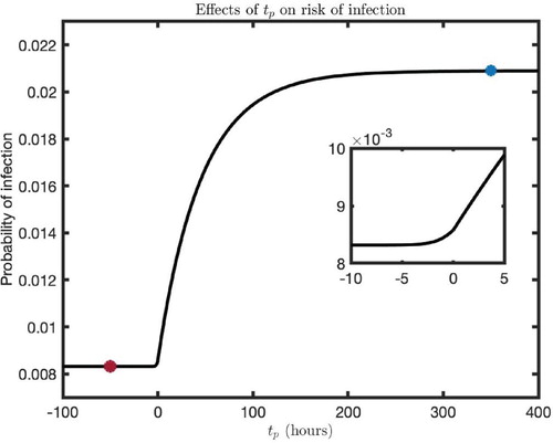
The probability of infection for the different timing of virus-exposure ($t_p$) predicted by our model is given in Figure 7. The level of probability before morphine intake ($t_p<0$) represents the risk of infection for individuals without drugs of abuse in their system (red filled circle, Figure 7). The presence of morphine gradually increases the risk of infection until it saturates at some steady-state level (Figure 7). The steady state of probability reached after morphine intake represents the risk of infection for individuals who experience prolonged conditions of drugs of abuse (blue-filled circle, Figure 7). For comparison, our model predicts that the risk of infection for a susceptible individual per sexual act is $0.83\mathrm{\%}$ in the absence of drugs of abuse while the risk increases to $2.09\mathrm{\%}$ for prolonged conditioning of drugs of abuse. Therefore, from a single exposure to virus, drug abusers can be 2.5 times more likely to get infected with HIV than those individuals without drugs of abuse. It is interesting to note that the probability is higher even before the morphine-intake (Figure 7 inset), showing that there is a higher risk of infection for drug abusers even when morphine is taken after virus exposure. This is due to the fact that the virus can remain long enough until the morphine taken later switches target cell populations.

Figure 7. Infection probability for the different timing of virus exposure ($t_p$). Note that $t_p=0$ represents the time of morphine intake. The red filled circle represents the risk of infection when morphine is absent, and the blue-filled circle is the maximum risk of infection for an individual under prolonged morphine conditioning. The following parameter values were used: $m=1.64\times {10}^{-5},c=23,{\beta }_l=5.13\times {10}^{-10},{\beta }_h=3.02\times {10}^{-8},p=2500,\delta =.38,r=0.5,q=4.42\times {10}^{-7},d=0.01$, $T_{l0}=6.1\times {10}^5$, and $T_{h0}=3.9\times {10}^5$.

5. Impact of preventive therapy

Antiretroviral therapy (ART) as preventive therapy, such as pre-exposure prophylaxis (PrEP) and post-exposure prophylaxis (PEP), has been commonly practiced. Currently the five classes of ART, nucleoside reverse transcriptase inhibitors (NRTI), nonnucleoside reverse transcriptase inhibitors (NNRTI), protease inhibitors (PI), fusion inhibitors (FI), and integrase inhibitors (II) [32,33], show their antiviral activity either by reducing the infection rate ${\beta }_l$ and ${\beta }_h$ to the rates $(1-\epsilon ){\beta }_l$ and $(1-\epsilon ){\beta }_h$, respectively, or the viral production rate, p, to the rate $(1-\eta )p$. Here, $\epsilon \in [0,1]$ and $\eta \in [0,1]$ represent the efficacy of ART to reduce infection rates and to reduce the virus production rate, respectively. These terms corresponding to ART efficacy affect our formulation of both $P_{\mathrm{cell}}$ and $P_{\mathrm{persist}}$.

5.1. Formulation of risk of infection under preventive therapy

We assume that the treatment begins at time $t_t$ such that $t_t\le t_p$ represents PrEP and $t_t>t_p$ represents PEP, where $t_p$ represents the time of virus exposure. Including the treatment conditions (${\beta }_l\to (1-\epsilon ){\beta }_l$, ${\beta }_h\to (1-\epsilon ){\beta }_h$, and $p\to (1-\eta )p$) into the formulation above, we obtain the probability of infection, $P_{\inf (\mathrm{PrEP})}$ and $P_{\inf (\mathrm{PEP})}$, for both cases, PrEP and PEP, respectively.

ART as pre-exposure prophylaxis (PrEP). When ART is used as PrEP, i.e. $t_t\le t_p$, we obtain (16) $P_{\mathrm{cell}(\mathrm{PrEP})}=1-e^{-m{V}_{\mathrm{donor}}\left({\int }_{t_p}^{\mathrm{\infty }}[(1-\epsilon ){\beta }_l{T}_l(s)+(1-\epsilon ){\beta }_h{T}_h(s)]e^{-c(s-t_p)}\mathrm{d}s\right),}$(16) where (17a) $\begin{array}{rl}{T}_h(t)& =\{\begin{array}{ll}{T}_{h0}& \mathrm{if}t<0,\\ {\displaystyle \frac{r{T}_0+[(d+q+r)T_{h0}-r{T}_0]e^{-(d+q+r)t}}{d+q+r}}& \mathrm{if}t\ge 0,\end{array}\end{array}$(17a) (17b) $\begin{array}{rl}{T}_l(t)& =T_0-T_h(t).\end{array}$(17b) In this case, the basic reproduction number under PrEP, $R_{0(\mathrm{PrEP})}$, is given by (18) $R_{0(\mathrm{PrEP})}=(1-\epsilon )(1-\eta )R_0,$(18) and the probability of persistence is given by (19) $P_{\mathrm{persist}(\mathrm{PrEP})}=1-e^{-R_{0(\mathrm{PrEP})}}$(19) Finally, with $P_{\mathrm{cell}(\mathrm{PrEP})}$ from Equation (16(16) $P_{\mathrm{cell}(\mathrm{PrEP})}=1-e^{-m{V}_{\mathrm{donor}}\left({\int }_{t_p}^{\mathrm{\infty }}[(1-\epsilon ){\beta }_l{T}_l(s)+(1-\epsilon ){\beta }_h{T}_h(s)]e^{-c(s-t_p)}\mathrm{d}s\right),}$(16) ) and $P_{\mathrm{persist}(\mathrm{PrEP})}$ from Equation (19(19) $P_{\mathrm{persist}(\mathrm{PrEP})}=1-e^{-R_{0(\mathrm{PrEP})}}$(19) ), we compute the risk of infection under PrEP using the following expression. (20) $P_{\inf (\mathrm{PrEP})}=P_{\mathrm{cell}(\mathrm{PrEP})}\cdot P_{\mathrm{persist}(\mathrm{PrEP})}.$(20)

ART as post-exposure prophylaxis (PEP). When ART is used as PEP, i.e. $t_t>t_p$, we obtain the probability that the infection is ultimately initiated (i.e. at least one cell is eventually infected) as (21) $P_{\mathrm{cell}(\mathrm{PEP})}=1-e^{-m{V}_{\mathrm{donor}}({\int }_{t_p}^{t_t}[{\beta }_l{T}_l(s)+{\beta }_h{T}_h(s)]e^{-c(s-t_p)}\mathrm{d}s+{\int }_{t_t}^{\mathrm{\infty }}[(1-\epsilon ){\beta }_l{T}_l(s)+(1-\epsilon ){\beta }_h{T}_h(s)]e^{-c(s-t_p)}\mathrm{d}s),}$(21) where (22a) $\begin{array}{rl}{T}_h(t)& =\{\begin{array}{ll}{T}_{h0}& \mathrm{if}t<0,\\ {\displaystyle \frac{r{T}_0+[(d+q+r)T_{h0}-r{T}_0]e^{-(d+q+r)t}}{d+q+r}}& \mathrm{if}t\ge 0,\end{array}\end{array}$(22a) (22b) $\begin{array}{rl}{T}_l(t)& =T_0-T_h(t).\end{array}$(22b)

In the case of PEP, there are two possibilities for an infection to occur: (1) the infection is initiated before the treatment begins ($t_i<t_t$), or (2) the infection is initiated after the treatment begins ($t_i\ge t_t$). The probability that the infection occurs before treatment begins $t_i<t_t$ is given by $AA=1-\exp (-m{V}_{\mathrm{donor}}{\int }_{t_p}^{t_t}{e}^{-c(s-t_p)}[{\beta }_l{T}_l(s)+{\beta }_h{T}_h(s)]\mathrm{d}s),$where (23a) $\begin{array}{rl}{T}_h(t)& =\{\begin{array}{ll}{T}_{h0}& \mathrm{if}t<0,\\ {\displaystyle \frac{r{T}_0+[(d+q+r)T_{h0}-r{T}_0]e^{-(d+q+r)t}}{d+q+r}}& \mathrm{if}t\ge 0,\end{array}\end{array}$(23a) (23b) $\begin{array}{rl}{T}_l(t)& =T_0-T_h(t),\end{array}$(23b) and the basic reproduction number for this case remains the same as above ($R_0$ in Equation (9(9) $R_0=\frac{p}{c\delta }[{\beta }_l{T}_l(t_p)+{\beta }_h{T}_h(t_p)],$(9) )). Thus, the probability of persistence under PEP if the infection occurs before treatment begins ($t_i<t_t$) is $P_{\mathrm{persist}(\mathrm{PEP}1)}=1-e^{-R_0}.$

Similarly, the probability that the infection is initiated after the treatment begins ($t_i\ge t_t$) is given by ($P_{\mathrm{cell}(\mathrm{PEP})}-AA$) and the corresponding basic reproduction number is (24) ${\hat{R}}_{0t}=\frac{(1-\eta )(1-\epsilon )p}{\delta c}[{\beta }_l{T}_l(t_t)+{\beta }_h{T}_h(t_t)].$(24) This implies that the probability of persistence under PEP if the infection occurs after treatment begins ($t_i\ge t_t$) is $P_{\mathrm{persist}(\mathrm{PEP}2)}=1-e^{-{\hat{R}}_{0t}}.$

Therefore, including both possibilities, we obtain the risk of infection in the case of PEP as follows: (25) $\begin{array}{rl}{P}_{\inf (\mathrm{PEP})}& =AA\cdot P_{\mathrm{persist}(\mathrm{PEP}1)}+[P_{\mathrm{cell}(\mathrm{PEP})}-AA]\cdot P_{\mathrm{persist}(\mathrm{PEP}2)}\\ & =AA(1-e^{-R_0})+[P_{\mathrm{cell}(\mathrm{PEP})}-AA](1-e^{-{\hat{R}}_{0t}}).\end{array}$(25)

5.2. Computation of risk of infection under preventive therapy

The net efficacy of treatment can be affected by many factors, such as the frequency of dosages, the timing of dosages, drug choice, and the timing relevant to virus exposure [13,43]. Strict abidance to PrEP guidelines have also been associated with increased treatment efficacy [37]. In general, the efficacy of a treatment is expected to be less than 100%; it typically has an effectiveness between 0% and 75% [2,11]. For the purpose of our computation, we chose values for both efficacies as $\epsilon =0.5$ and $\eta =0.5$ which falls in line with [5].

The impact of PrEP/PEP on the probability of infection predicted by our model (Equations (20(20) $P_{\inf (\mathrm{PrEP})}=P_{\mathrm{cell}(\mathrm{PrEP})}\cdot P_{\mathrm{persist}(\mathrm{PrEP})}.$(20) ) and (25(25) $\begin{array}{rl}{P}_{\inf (\mathrm{PEP})}& =AA\cdot P_{\mathrm{persist}(\mathrm{PEP}1)}+[P_{\mathrm{cell}(\mathrm{PEP})}-AA]\cdot P_{\mathrm{persist}(\mathrm{PEP}2)}\\ & =AA(1-e^{-R_0})+[P_{\mathrm{cell}(\mathrm{PEP})}-AA](1-e^{-{\hat{R}}_{0t}}).\end{array}$(25) )) is shown in Figure 8. The graphs shown are the infection probability for the different timings of treatment initiation pre-/post-virus exposure ($t_t-t_p$) in an individual without (red) and with (blue) prolonged conditioning of drugs of abuse (Figure 8). Note that $t_t-t_p=0$ represents PrEP and $t_t-t_p>0$ represents PEP. Comparing two individuals taking PrEP, one with morphine in their system and another without, we observe quite different risks of infection between them. An individual without drugs of abuse and taking PrEP has a risk of infection of 0.2% while an individual using drugs of abuse and taking PrEP has a risk of infection of 0.9%, a 4.5 times higher risk of infection. Also, in the case of both PrEP and PEP, the risk of infection always remains higher in individuals with conditioning of drugs of abuse (Figure 8). In fact, the individual using drugs of abuse while taking PrEP has a higher risk of infection than an individual without drugs of abuse who never seeks preventive therapy.

Figure 8. Infection probability for the different timings of treatment initiation pre-/post-virus exposure ($t_t-t_p$). Note that $t_t-t_p=0$ represents PrEP and $t_t-t_p>0$ represents PEP. We considered two cases: the absence of drugs of abuse (red curve) and prolonged presence of drugs of abuse (blue curve). The parameter values used were as follows: $m=1.64\times {10}^{-5},c=23,{\beta }_l=5.13\times {10}^{-10},{\beta }_h=3.02\times {10}^{-8},p=2500,\delta =.38,r=0.5,q=4.42\times {10}^{-7},d=0.01,T_{l0}=6.1\times {10}^5,T_{h0}=3.9\times {10}^5,\epsilon =0.5$ and $\eta =\mathrm{0.5.}$

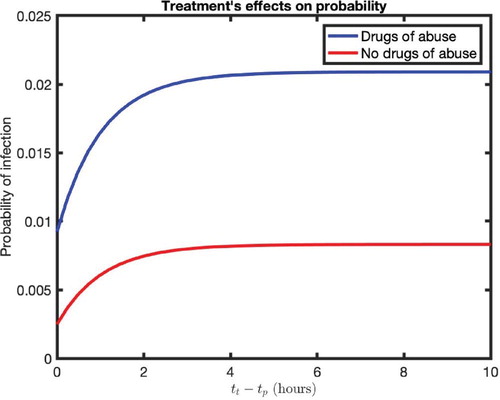
Previous studies have shown that the early initiation of antiretroviral therapy can significantly reduce rates of transmission of HIV [7,28]. However, it is commonly unknown what defines early and when treatment no longer affects the risk of infection [14]. Our model predicts that an increase in $t_t-t_p$ (delay in treatment post-virus exposure), increases the risk of infection in both cases (with/without drugs of abuse). We found that the risk of infection reaches a maximum value at approximately $t_t-t_p=4$ hours for both individuals. Therefore, delay of treatment initiation more than 4 hours from virus exposure may not be as effective as beginning PEP earlier.

We now observe how the risk of infection changes when the effectiveness of treatment (ϵ and η) are varied. The risk of infection predicted for different efficacy levels of PrEP ($t_t-t_p=0$) is presented in Figure 9 (left). With an increase in efficacy of PrEP, the risk of infection is estimated to be decreased for both individuals with and without conditioning of drugs of abuse. However, the risk of infection under drugs of abuse remains higher for any efficacy of treatment; even at the $75\mathrm{\%}$ effective level of PrEP (the highest level considered), the risk of infection for an individual with drugs of abuse in their system is 5.2 times higher than an individual without drugs of abuse.

Figure 9. (left) Risk of infection under PrEP $(t_t-t_p=0)$ and (right) the delay in treatment initiation $(t_t-t_p$) causing the risk of infection at its maximum value, for various treatment efficacies. All other parameters are the same as in Figure 8.

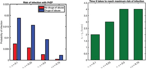
For PEP ($t_t-t_p>0$), the risk of infection increases as the initiation of treatment is delayed longer (i.e. $t_t-t_p$ higher) and eventually reaches the maximum risk of infection for long enough delay (Figure 8 right). It is important to identify how the varying efficacy of treatment affects the amount of minimum delay in treatment that causes the risk of infection at its maximum value. As shown in Figure 9 (right), with a $10\mathrm{\%}$ efficacy of treatment, the maximum risk is reached if treatment is delayed for longer than 2 hours. As the effectiveness of the treatment increases, the delay in treatment, for which the risk is at maximum value, also increases. For example, with $25\mathrm{\%}$ and $50\mathrm{\%}$ efficacies, an individual has a three-hour and four-hour window of opportunity, respectively, to begin treatment to maintain a risk of infection lower than its maximum value.

6. Discussion

In this study, we develop a mathematical model which allows us to quantify the risk of HIV infection in individuals under conditioning of drugs of abuse. This model illustrates the impact of complex biological alteration due to drugs of abuse such as morphine can have on HIV infection and the risk of its transmission. In particular, analyzing the virus dynamics under morphine conditioning, our model demonstrates that because morphine alters co-receptor expression in target cells, individuals under morphine conditioning can have a substantially higher proportion of high susceptible target cells (CD4 T cells). We found this proportion to be $39\mathrm{\%}$ in the absence of morphine vs. $98\mathrm{\%}$ under a prolonged exposure to morphine, indicating higher risk of infection in drug abusers. Moreover, the proportion of high susceptible cells is mostly amplified by the transition rate of CD4 T cells from the low to the high susceptible category, r, which depends on the presence of morphine. Using a thorough analysis of deterministic models along with a probabilistic approach, we have successfully formulated a risk of infection for an uninfected drug abuser after a single contact with an HIV-infected partner.

Our model predicts that the prolonged conditioning of drugs of abuse in individuals can cause a 2.5-fold higher risk of infection per sexual contact (0.83% without drugs of abuse vs. 2.09% under drugs of abuse). Importantly, the amount of increase in the risk of infection in drug abusers highly depends upon the duration of time between morphine intake and virus exposure; the longer the morphine stays in the body before virus exposure, the higher the risk of infection. An increase in the risk of infection is observed even in the case when morphine is taken after virus exposure. In our base case computation, when virus is introduced up to four hours before morphine intake, the risk of infection can be increased. This interesting phenomena of increase in the risk of infection even with morphine intake after the virus exposure is because the virus may still survive until the time of morphine intake causing the target cells switch to higher susceptibility. While these results are obtained based on parameters related to sexual transmission, the model can easily be adjusted to predict the risk of infection through other routes of transmission, such as injection drug use, by choosing the appropriate value of transmission-related parameter m.

We also implemented our models to evaluate the effects of preventive therapy (PrEP and PEP) on reducing the risk of infection. Our model predicts that the timing of treatment initiation is highly critical in both cases, with and without drugs of abuse. For example, as revealed in our computation with the $50\mathrm{\%}$ efficacy level, if an individual doesn't begin treatment within 4 h of virus exposure, the probability of infection might have already reached its maximum value and the treatment may not be as effective as an earlier initiation of PEP. This shows that there is a time-window of opportunity (i.e., minimum delay for treatment initiation after virus exposure) during which the treatment should be initiated to assure the reduced risk of infection, increasing the chance for HIV prevention. In general, we observe that the time-window of opportunity is wider for a higher efficacy of PEP. This result may explain why the PEP begun as early as 3 days post-infection in a recent study [47] on monkey experiments could not prevent the SIV (simian immunodeficiency virus) infection.

Using the model to compute the two cases of individuals taking PrEP with a $50\mathrm{\%}$ efficacy, one without drugs of abuse and the other under drugs of abuse, the individuals with the drugs of abuse have a predicted risk 4.5 times higher than the other individuals. A similar effect was observed in the case of $50\mathrm{\%}$ effective PEP, in which the risk of infection always remains higher (up to 2.5 times) in individuals with drugs of abuse, compared to individuals without the conditioning of drugs of abuse. This trend holds true with varying efficacies of treatment as well. For example, an individual under drugs of abuse using PrEP with a $75\mathrm{\%}$ efficacy has the risk of infection approximately the same as an individual without drugs of abuse using a $50\mathrm{\%}$ effective PrEP. The significant higher risk of infection for the drug abusers than the individuals not using drugs of abuse can partly explain the high percentage of drug abusers contracting HIV.

We acknowledge several limitations of our model. Our computation is based on the parameters estimated from the limited study on drugs of abuse. Therefore, some of our quantitative predictions may need the further evaluation with rich data sets. We used a constant morphine concentration rather than a time-varying concentration as the body clears the morphine from the system over time. The model also assumes a constant treatment efficacy, however, the treatment concentration within the body decreases overtime between doses, or efficacy of the treatment changes if doses are missed. Further analysis on these limitations allows for higher resolution of probability of infection predicted by the models. Also, we have considered only CD4 T cells as a target for HIV infection and have ignored the possibility of infecting other immune cells such as macrophages and dendritic cells. Extended models including all of these cells may help to predict a more accurate probability of infection. However, such models require more reliable parameters related to additional cells under morphine. As the effectiveness of the transfer of T cells and other immune cells from the infected source partner is not well understood, we did not consider transfer of these cells from the source partner and have only considered the viruses that reach the target cell site of the recipient individual.

In summary, we developed a mathematical model to compute the risk of infection for drug abusers, including those who are under preventive therapy. With a more comprehensive understanding of the risk of infection for individuals under drugs of abuse, strides can be made towards improving therapy guidelines and regulations. These results can be helpful for medical professionals and policy makers to design more effective treatment protocols for the control and prevention of HIV transmission in drug abusers.

Acknowledgments

This work was funded by NSF grants DMS-1951793, DMS-1616299, DMS-1836647, and DEB-2030479 from National Science Foundation of USA, and UGP award and the start-up fund from San Diego State University.

Disclosure statement

No potential conflict of interest was reported by the authors.

Additional information

Funding

This work was supported by National Science Foundation of USA [grant numbers DMS-1951793, DMS-1616299, DMS- 1836647, DEB-2030479] and San Diego State University [grant number UGP Award, Start-up].

Appendices

Appendix 1. Proof of Theorem 3.1

Jacobian of the model system (7(7) $\begin{array}{rl}\dot{T_l}& =\lambda -\mathrm{d}{T}_l-r{T}_l-{\beta }_l{T}_{l}V+q{T}_h,\\ \dot{T_h}& =r{T}_l-\mathrm{d}{T}_h-{\beta }_h{T}_{h}V-q{T}_h,\\ \dot{I}& ={\beta }_l{T}_{l}V+{\beta }_h{T}_{h}V-\delta I,\\ \dot{V}& =pI-cV,\end{array}$(7) ) is given by $J=\left[\begin{array}{cccc}-d-r-{\beta }_{l}V& q& 0& -{\beta }_{l}Tl\\ r& -d-q-{\beta }_{h}V& 0& -{\beta }_{h}Th\\ {\beta }_{l}V& {\beta }_{h}V& -\delta & {\beta }_{l}Tl+{\beta }_{h}Th\\ 0& 0& p& -c\end{array}\right]$Linearizing the Jacobian around the IFE, we get $J{|}_{\mathrm{IFE}}=\left[\begin{array}{cc}{X}_{2\times 2}& Y_{2\times 2}\\ O_{2\times 2}& Z_{2\times 2}\end{array}\right],$where $\begin{array}{rl}& X=\left[\begin{array}{cc}-d-r& q\\ r& -d-q\end{array}\right],Y=\left[\begin{array}{cc}0& -{\beta }_l{\displaystyle \frac{\lambda (d+q)}{d(d+q+r)}}\\ 0& -{\beta }_h{\displaystyle \frac{\lambda r}{d(d+q+r)}}\end{array}\right],\\ & Z=\left[\begin{array}{cc}-\delta & {\beta }_l{\displaystyle \frac{\lambda (d+q)}{d(d+q+r)}}+{\beta }_h{\displaystyle \frac{\lambda r}{d(d+q+r)}}\\ p& -c\end{array}\right].\end{array}$Here, the eigenvalues of $J{|}_{\mathrm{IFE}}$ are given by the eigenvalues of the block matrices X and Z. Since $\mathrm{trace}(X)=-2d-r-q<0$, and $\det (X)=d(d+q+r)>0$, the eigenvalues of X are negative. Similarly, $\mathrm{trace}(Z)=-\delta -c<0$, and $\det (Z)=\delta c(1-R_0)$, which is positive if $R_0<1$. Therefore, the eigenvalues of Z are negative if $R_0<1$. This implies that all eigenvalues of $J{|}_{\mathrm{IFE}}$ are negative if $R_0<1$. Hence, if $R_0<1,$ the IFE is locally asymptotically stable, and if $R_0>1$, the IFE is unstable.

Appendix 2. Proof of Theorem 3.2

The infection-free equilibrium of the system (7(7) $\begin{array}{rl}\dot{T_l}& =\lambda -\mathrm{d}{T}_l-r{T}_l-{\beta }_l{T}_{l}V+q{T}_h,\\ \dot{T_h}& =r{T}_l-\mathrm{d}{T}_h-{\beta }_h{T}_{h}V-q{T}_h,\\ \dot{I}& ={\beta }_l{T}_{l}V+{\beta }_h{T}_{h}V-\delta I,\\ \dot{V}& =pI-cV,\end{array}$(7) ) is given by $\mathrm{IFE}=(T_l^{\ast },T_h^{\ast },0,0)$, where $T_l^{\ast }=\frac{\lambda (d+q)}{d(d+q+r)}$ and $T_h^{\ast }=\frac{\lambda r}{d(d+q+r)}$. The Jacobian corresponding to the infectious equations (i.e. I and V equations) at IFE is $J1=\left[\begin{array}{cc}-\delta & {\beta }_l{T}_l^{\ast }+{\beta }_h{T}_h^{\ast }\\ p& -c\end{array}\right].$We define $s(R)=max\{\mathrm{Re}(\sigma ):\sigma \mathrm{is}\mathrm{an}\mathrm{eigenvalue}\mathrm{of}\mathrm{R}\}$. Clearly, $J1$ is an irreducible matrix with non-negative off-diagonal elements, thus we conclude that $s(J1)$ is a simple eigenvalue of $J1$ with a positive eigenvector [36].

From the local asymptotically stability proof, we have the following statements:

1. $R_0=1$ if and only if $s(J1)=0$;

2. $R_0>1$ if and only if $s(J1)>0$;

3. $R_0<1$ if and only if $s(J1)<0$.

Therefore, assuming $R_0<1$, we obtain that $s(J1)<0.$ Thus, we can find a sufficiently small positive value ${\rho }_0$ such that $s(J{1}_{{\rho }_0})<0$, where $J{1}_{{\rho }_0}=\left[\begin{array}{cc}-\delta & {\beta }_l(T_l^{\ast }+{\rho }_0)+{\beta }_h(T_h^{\ast }+{\rho }_0)\\ p& -c\end{array}\right]$From the system (7(7) $\begin{array}{rl}\dot{T_l}& =\lambda -\mathrm{d}{T}_l-r{T}_l-{\beta }_l{T}_{l}V+q{T}_h,\\ \dot{T_h}& =r{T}_l-\mathrm{d}{T}_h-{\beta }_h{T}_{h}V-q{T}_h,\\ \dot{I}& ={\beta }_l{T}_{l}V+{\beta }_h{T}_{h}V-\delta I,\\ \dot{V}& =pI-cV,\end{array}$(7) ), we have (A1) $\begin{array}{rl}\dot{T_l}& \le \lambda -\mathrm{d}{T}_l-r{T}_l+q{T}_h,\\ \dot{T_h}& \le r{T}_l-\mathrm{d}{T}_h-q{T}_h.\end{array}$(A1) This implies $\underset{t\to \mathrm{\infty }}{lim}{T}_l(t)\le T_l^{\ast }$ and $\underset{t\to \mathrm{\infty }}{lim}{T}_h(t)\le T_h^{\ast }$. Then, there exists a $t_1>0$, such that $\mathrm{\forall }t\ge t_1$, (A2) $\begin{array}{rl}{T}_l(t)& \le T_l^{\ast }+{\rho }_0,\\ T_h(t)& \le T_h^{\ast }+{\rho }_0.\end{array}$(A2) Using the infectious equations of system (7(7) $\begin{array}{rl}\dot{T_l}& =\lambda -\mathrm{d}{T}_l-r{T}_l-{\beta }_l{T}_{l}V+q{T}_h,\\ \dot{T_h}& =r{T}_l-\mathrm{d}{T}_h-{\beta }_h{T}_{h}V-q{T}_h,\\ \dot{I}& ={\beta }_l{T}_{l}V+{\beta }_h{T}_{h}V-\delta I,\\ \dot{V}& =pI-cV,\end{array}$(7) ) for $t\ge t_1$, we obtain the following: (A3) $\begin{array}{rl}\dot{I}& \le V[{\beta }_l(T_l^{\ast }+{\rho }_0)+{\beta }_h(T_h^{\ast }+{\rho }_0)]-\delta I,\\ \dot{V}& =pI-cV.\end{array}$(A3) We now consider the auxiliary system for $t\ge t_1$ (A4) $\begin{array}{rl}\dot{I}& =-\delta I+[{\beta }_l(T_l^{\ast }+{\rho }_0)+{\beta }_h(T_h^{\ast }+{\rho }_0)]V,\\ \dot{V}& =pI-cV.\end{array}$(A4) Since $J{1}_{{\rho }_0}$ is irreducible with non-negative off-diagonal elements we have that $s(J{1}_{{\rho }_0})$ is associated with a strongly positive eigenvector $\tilde{v}\in {\mathbb{R}}^2$ [36]. For any solution $T_l(t),T_h(t),I(t),V(t)$ of system (7(7) $\begin{array}{rl}\dot{T_l}& =\lambda -\mathrm{d}{T}_l-r{T}_l-{\beta }_l{T}_{l}V+q{T}_h,\\ \dot{T_h}& =r{T}_l-\mathrm{d}{T}_h-{\beta }_h{T}_{h}V-q{T}_h,\\ \dot{I}& ={\beta }_l{T}_{l}V+{\beta }_h{T}_{h}V-\delta I,\\ \dot{V}& =pI-cV,\end{array}$(7) ), with a non-negative initial condition $T_l(t_i),T_h(t_i),I(t_i),V(t_i)$, we can find a sufficiently large b>0, such that $(I(t_1),V(t_1))\le b\tilde{v}.$ It is easy to see that $H(t)=b{e}^{s(J{1}_{{\rho }_0})(t-t_1)}\tilde{v}$ is a solution of the auxiliary system (A4) with $H(t_1)=b\tilde{v}$. Using the comparison principle [36], we conclude that $(I(t),V(t))\le b{e}^{s(J{1}_{{\rho }_0})(t-t_1)}\tilde{v},\mathrm{\forall }t\ge t_1.$And because $s(J{1}_{{\rho }_0})<0$, we can conclude (A5) $\underset{t\to \mathrm{\infty }}{lim}(I(t),V(t))=(0,0).$(A5) It then follows that $T_l$ and $T_h$ are asymptotic to the following system: (A6) $\begin{array}{rl}\dot{T_l}& =\lambda -\mathrm{d}{T}_l-r{T}_l+q{T}_h,\end{array}$(A6) (A7) $\begin{array}{rl}\dot{T_h}& =r{T}_l-\mathrm{d}{T}_h-q{T}_h.\end{array}$(A7) and using the asymptotically autonomous semiflows theory [41], we have the following: (A8) $\begin{array}{rl}& \underset{t\to \mathrm{\infty }}{lim}{T}_l(t)=T_l^{\ast }\\ & \underset{t\to \mathrm{\infty }}{lim}{T}_h(t)=T_h^{\ast }\end{array}$(A8) Now combining Equations (A5) and (A8), we have $\underset{t\to \mathrm{\infty }}{lim}(T_l(t),T_h(t),I(t),V(t))=(T_l^{\ast },T_h^{\ast },0,0).$This proves that the IFE is globally attractive in ${\mathbb{R}}^4$ if $R_0<1$. Thus, the IFE is globally asymptotically stable if $R_0<1.$

Appendix 3. Proof of Theorem 3.3

If $R_0>1$, we obtain $s(J1)>0$. Suppose $\mathcal{P}(t)H$ is the solution maps generated by the system (7(7) $\begin{array}{rl}\dot{T_l}& =\lambda -\mathrm{d}{T}_l-r{T}_l-{\beta }_l{T}_{l}V+q{T}_h,\\ \dot{T_h}& =r{T}_l-\mathrm{d}{T}_h-{\beta }_h{T}_{h}V-q{T}_h,\\ \dot{I}& ={\beta }_l{T}_{l}V+{\beta }_h{T}_{h}V-\delta I,\\ \dot{V}& =pI-cV,\end{array}$(7) ) with initial value H. Here, the system, $\{\mathcal{P}(t){\}}_{t\ge 0}$ admits a global attractor in $\mathbb{X}={\mathbb{R}}_{+}^4$ [20]. We now prove that $\{\mathcal{P}(t){\}}_{t\ge 0}$ is uniformly persistent with respect to $({\mathbb{X}}_0,\mathrm{\partial }{\mathbb{X}}_0)$, where ${\mathbb{X}}_0:=\{(T_l,T_h,I,V)\in \mathbb{X}:I>0\text{and}V>0\},$and $\mathrm{\partial }{\mathbb{X}}_0:=\mathbb{X}\mathrm{\setminus }{\mathbb{X}}_0=\{(T_l,T_h,I,V)\in \mathbb{X}:I=0\text{or}V=0\}.$Given any initial value $(T_{l0},T_{h0},I_0,V_0)\in {\mathbb{X}}_0$, from the first equation of the system (7(7) $\begin{array}{rl}\dot{T_l}& =\lambda -\mathrm{d}{T}_l-r{T}_l-{\beta }_l{T}_{l}V+q{T}_h,\\ \dot{T_h}& =r{T}_l-\mathrm{d}{T}_h-{\beta }_h{T}_{h}V-q{T}_h,\\ \dot{I}& ={\beta }_l{T}_{l}V+{\beta }_h{T}_{h}V-\delta I,\\ \dot{V}& =pI-cV,\end{array}$(7) ), we get (A9) $T_l(t)=e^{-{\int }_0^{t}b(s_1)\mathrm{d}{s}_1}[{\int }_0^t{e}^{{\int }_0^{s_2}b(s_1)\mathrm{d}{s}_1}a(s_2)\mathrm{d}{s}_2+T_{l0}],$(A9) where (A10) $a(t):=\lambda +q{T}_h(t)\ge \lambda >0,$(A10) and (A11) $b(t):=d+r+{\beta }_{l}V(t).$(A11) Thus, $T_l(t)>0,\mathrm{\forall }t>0$. Also, from the second equation of system (7(7) $\begin{array}{rl}\dot{T_l}& =\lambda -\mathrm{d}{T}_l-r{T}_l-{\beta }_l{T}_{l}V+q{T}_h,\\ \dot{T_h}& =r{T}_l-\mathrm{d}{T}_h-{\beta }_h{T}_{h}V-q{T}_h,\\ \dot{I}& ={\beta }_l{T}_{l}V+{\beta }_h{T}_{h}V-\delta I,\\ \dot{V}& =pI-cV,\end{array}$(7) ), we get (A12) $T_h(t)=e^{-{\int }_0^t\hat{b}(s_1)\mathrm{d}{s}_1}[{\int }_0^t{e}^{{\int }_0^{s_2}\hat{b}(s_1)\mathrm{d}{s}_1}\hat{a}(s_2)\mathrm{d}{s}_2+T_{h0}],$(A12) where (A13) $\hat{a}(t):=r{T}_l(t)>0,$(A13) and (A14) $\hat{b}(t):=d+q+{\beta }_{h}V(t).$(A14) Thus, $T_h(t)>0,\mathrm{\forall }t>0$.

Treating Theorem 4.1.1 of [34] as generalized to nonautonomous systems, the irreducibility of the cooperative matrix (A15) $C=\left[\begin{array}{cc}-\delta & {\beta }_l{T}_l(t)+{\beta }_h{T}_h(t)\\ p& -c\end{array}\right]$(A15) implies that (A16) $(I(t),V(t){)}^T\gg 0,\mathrm{\forall }t>0.$(A16) Therefore, we have the following lemma.

Lemma A.1

Assuming that $(T_l(t),T_h(t),I(t),V(t))$ is a solution of the system (7(7) $\begin{array}{rl}\dot{T_l}& =\lambda -\mathrm{d}{T}_l-r{T}_l-{\beta }_l{T}_{l}V+q{T}_h,\\ \dot{T_h}& =r{T}_l-\mathrm{d}{T}_h-{\beta }_h{T}_{h}V-q{T}_h,\\ \dot{I}& ={\beta }_l{T}_{l}V+{\beta }_h{T}_{h}V-\delta I,\\ \dot{V}& =pI-cV,\end{array}$(7) ) with initial value $(T_{l0},T_{h0},I_0,V_0)\in {\mathbb{X}}_0$, we have the following $(T_l(t),T)h(t),I(t),V(t))\gg 0,t>0.$

Lemma A.1 implies that ${\mathbb{X}}_0$ and $\mathrm{\partial }{\mathbb{X}}_0$ are positively invariant. Clearly, ${\mathbb{X}}_0\cup \mathrm{\partial }{\mathbb{X}}_0=\mathbb{X},{\mathbb{X}}_0\cap \mathrm{\partial }{\mathbb{X}}_0=\varnothing$ and $\mathrm{\partial }{\mathbb{X}}_0$ is relatively closed in $\mathbb{X}$.

Let $M_{\mathrm{\partial }}=\{(T_{l0},T_{h0},I_0,V_0)\in \mathrm{\partial }{\mathbb{X}}_0:\mathcal{P}(t)(T_{l0},T_{h0},I_0,V_0)\in \mathrm{\partial }{\mathbb{X}}_0,\mathrm{\forall }t\ge 0\}.$Then, we claim that (A17) $M_{\mathrm{\partial }}:=\{(T_{l0},T_{h0},I_0,V_0)\in \mathbb{X}:I_0=V_0=0\}.$(A17) In order to prove this claim, it is sufficient to show that for any $(T_{l0},T_{h0},I_0,V_0)\in M_{\mathrm{\partial }}$, $(I(t),V(t))=(0,0)$ $\mathrm{\forall }t$. If this does not hold true, then there exists a $t_2$ such that $(I(t_2),V(t_2))\ne (0,0)$. Since the matrix C (Equation (A15)) is irreducible with non-negative off-diagonal elements, $s(J1)$ is simple with an associated strongly positive eigenvector. Thus, it follows that $(I(t_2),V(t_2))\gg (0,0),\mathrm{\forall }t\ge t_2,$which is a contradiction to the definition of $M_{\mathrm{\partial }}$. Thus, we conclude that A17 is correct.

Clearly, there exists a unique fixed point of $\mathcal{P}(t)$ in $M_{\mathrm{\partial }}$ which is the $E_0=(T_l^{\ast },T_h^{\ast },0,0)$. So if $(T_l(t),T)h(t),I(t),V(t))$ is a non-negative solution of our system in $M_{\mathrm{\partial }}$, it is clear that every forward orbit of $\mathcal{P}(t)$ in $M_{\mathrm{\partial }}$ converges to $E_0$ as $t\to \mathrm{\infty }$, which is isolated in ${\mathbb{R}}_{+}^4$. Defining $W^s(E_0)$ as the stable manifold set of $E_0$, we have $W^s(E_0)\cap {\mathbb{X}}_0=\varnothing$ [35]. It is obvious that there is no cycle in $M_{\mathrm{\partial }}$ from $E_0$ to $E_0$. By Theorem 1.3.1 in [49], we conclude that the system (7(7) $\begin{array}{rl}\dot{T_l}& =\lambda -\mathrm{d}{T}_l-r{T}_l-{\beta }_l{T}_{l}V+q{T}_h,\\ \dot{T_h}& =r{T}_l-\mathrm{d}{T}_h-{\beta }_h{T}_{h}V-q{T}_h,\\ \dot{I}& ={\beta }_l{T}_{l}V+{\beta }_h{T}_{h}V-\delta I,\\ \dot{V}& =pI-cV,\end{array}$(7) ) is uniformly persistent with respect to $({\mathbb{X}}_0,\mathrm{\partial }{\mathbb{X}}_0)$. More specifically, there exists a positive constant $\xi >0$ such that conditions (11(11) $\underset{t\to \mathrm{\infty }}{lim}infI(t)\ge \xi ,\underset{t\to \mathrm{\infty }}{lim}infV(t)\ge \xi .$(11) ) hold.

By Theorem 1.3.7 of [49], system (7(7) $\begin{array}{rl}\dot{T_l}& =\lambda -\mathrm{d}{T}_l-r{T}_l-{\beta }_l{T}_{l}V+q{T}_h,\\ \dot{T_h}& =r{T}_l-\mathrm{d}{T}_h-{\beta }_h{T}_{h}V-q{T}_h,\\ \dot{I}& ={\beta }_l{T}_{l}V+{\beta }_h{T}_{h}V-\delta I,\\ \dot{V}& =pI-cV,\end{array}$(7) ) has at least one equilibrium $(\widehat{T_l},\widehat{T_h},\hat{I},\hat{V})\in {\mathbb{X}}_0$, where $\hat{I}>0$ and $\hat{V}>0$. Thus, we can conclude that $(\widehat{T_l},\widehat{T_h},\hat{I},\hat{V})$ is a positive equilibrium of system (7(7) $\begin{array}{rl}\dot{T_l}& =\lambda -\mathrm{d}{T}_l-r{T}_l-{\beta }_l{T}_{l}V+q{T}_h,\\ \dot{T_h}& =r{T}_l-\mathrm{d}{T}_h-{\beta }_h{T}_{h}V-q{T}_h,\\ \dot{I}& ={\beta }_l{T}_{l}V+{\beta }_h{T}_{h}V-\delta I,\\ \dot{V}& =pI-cV,\end{array}$(7) ). Further computation allows us to find the following closed form of the positive equilibrium. $\begin{array}{rl}\widehat{T_l}& =\frac{\delta c}{{\beta }_{l}p}-\frac{{\beta }_h\widehat{T_h}}{{\beta }_l}\\ \widehat{T_h}& =\frac{c\mathrm{d}\delta -{\beta }_l\lambda p}{p({\beta }_{h}d-{\beta }_{l}d)}-\frac{({\beta }_{h}c\mathrm{d}\delta -{\beta }_h{\beta }_l\lambda p-\sqrt{\mathrm{\Psi }}+{\beta }_{l}c\mathrm{d}\delta +{\beta }_{l}c\delta q+{\beta }_{h}c\delta r)}{2{\beta }_{h}p({\beta }_{h}d-{\beta }_{l}d)}\\ \hat{I}& =\frac{c\hat{V}}{p}\\ \hat{V}& =-\frac{{\beta }_{h}c\mathrm{d}\delta -{\beta }_h{\beta }_l\lambda p-\sqrt{\mathrm{\Psi }}+{\beta }_{l}c\mathrm{d}\delta +{\beta }_{l}c\delta q+{\beta }_{h}c\delta r}{2{\beta }_h{\beta }_{l}c\delta }\end{array}$where Ψ is defined as $\begin{array}{rl}\mathrm{\Psi }& ={\beta }_h^2{\beta }_l^2{\lambda }^2{p}^2-2{\beta }_h^2{\beta }_{l}c\mathrm{d}\delta {\lambda }_p+2{\beta }_h^2{\beta }_{l}c\delta \lambda pr+{\beta }_h^2{c}^2{d}^2{\delta }^2+2{\beta }_h^2{c}^2\mathrm{d}{\delta }^{2}r+{\beta }_h^2{c}^2{\delta }^2{r}^2\\ & +2{\beta }_h{\beta }_l^{2}cd\delta \lambda p+2{\beta }_h{\beta }_l^{2}c\delta \lambda pq-2{\beta }_h{\beta }_l{c}^2{d}^2{\delta }^2-2{\beta }_h{\beta }_l{c}^2\mathrm{d}{\delta }^{2}q-2{\beta }_h{\beta }_l{c}^2\mathrm{d}{\delta }^{2}r+2{\beta }_h{\beta }_l{c}^2{\delta }^{2}qr\\ & +{\beta }_l^2{c}^2{d}^2{\delta }^2+2{\beta }_l^2{c}^2\mathrm{d}{\delta }^{2}q+{\beta }_l^2{c}^2{\delta }^2{q}^2\end{array}$

References

- L.J. Allen, An Introduction to Stochastic Processes with Applications to Biology, Chapman and Hall/CRC, New York, 2010.
- K.R. Amico and M.J. Stirratt, Adherence to preexposure prophylaxis: current, emerging, and anticipated bases of evidence, Clin. Infect. Dis. 59(suppl_1) (2014), pp. S55–S60. doi: 10.1093/cid/ciu266
- S. Bonhoeffer, R.M. May, G.M. Shaw, and M.A. Nowak, Virus dynamics and drug therapy, Proc. Natl Acad. Sci. 94(13) (1997), pp. 6971–6976. doi: 10.1073/pnas.94.13.6971
- L.S. Brown Jr, S.A. Kritz, R.J. Goldsmith, E.J. Bini, J. Rotrosen, S. Baker, J. Robinson, and P.McAuliffe, Characteristics of substance abuse treatment programs providing services for HIV/AIDS, hepatitis c virus infection, and sexually transmitted infections: The national drug abuse treatment clinical trials network, J. Subst. Abuse Treat. 30(4) (2006), pp. 315–321. doi: 10.1016/j.jsat.2006.02.006
- K. Choopanya, M. Martin, P. Suntharasamai, U. Sangkum, P.A. Mock, M. Leethochawalit, S.Chiamwongpaet, P. Kitisin, P. Natrujirote, S. Kittimunkong, and R. Chuachoowong, Antiretroviral prophylaxis for HIV infection in injecting drug users in Bangkok, Thailand (the Bangkok tenofovir study): a randomised, double-blind, placebo-controlled phase 3 trial, Lancet 381(9883) (2013), pp. 2083–2090. doi: 10.1016/S0140-6736(13)61127-7
- T.J. Cicero, M.S. Ellis, and Z.A. Kasper, Increased use of heroin as an initiating opioid of abuse, Addict. Behav. 74 (2017), pp. 63–66. doi: 10.1016/j.addbeh.2017.05.030
- M.S. Cohen, Y.Q. Chen, M. McCauley, T. Gamble, M.C. Hosseinipour, N. Kumarasamy, J.G. Hakim, J. Kumwenda, B. Grinsztejn, J.H. Pilotto, and S.V. Godbole, Prevention of HIV-1 infection with early antiretroviral therapy, N Eng J. Med. 365(6) (2011), pp. 493–505. doi: 10.1056/NEJMoa1105243
- N. Dalal, D. Greenhalgh, and X. Mao, A stochastic model for internal HIV dynamics, J. Math. Anal. Appl. 341(2) (2008), pp. 1084–1101. ISSN 0022-247X. doi:https://doi.org/10.1016/j.jmaa.2007.11.005.
- J.S. Fennema, E.J. Van Ameijden, A. van den Hoek, and R.A. Coutinho, Young and recent-onset injecting drug users are at higher risk for HIV, Addiction 92(11) (1997), pp. 1457–1465. doi: 10.1111/j.1360-0443.1997.tb02867.x
- H. Francis, Substance abuse and HIV infection, Topics HIV Med. Pub. Int. AIDS Soc. USA 11(1) (2003), pp. 20–24.
- R.H. Gray, X. Li, M.J. Wawer, S.J. Gange, D. Serwadda, N.K. Sewankambo, R. Moore, F.Wabwire-Mangen, T. Lutalo, and T.C. Quinn, Stochastic simulation of the impact of antiretroviral therapy and HIV vaccines on HIV transmission; Rakai, Uganda, Aids 17(13) (2003), pp. 1941–1951. doi: 10.1097/00002030-200309050-00013
- C.-J. Guo, Y. Li, S. Tian, X. Wang, S.D. Douglas, and W.-Z. Ho, Morphine enhances HIV infection of human blood mononuclear phagocytes through modulation of beta-chemokines and CCR5 receptor, J. Invest. Med. 50(6) (2002), pp. 435–442. ISSN 1081-5589. doi:10.1136/jim-50-06-03.
- J.E. Haberer, D.R. Bangsberg, J.M. Baeten, K. Curran, F. Koechlin, K.R. Amico, P. Anderson, N.Mugo, F. Venter, P. Goicochea, and C. Caceres, Defining success with HIV pre-exposure prophylaxis: a prevention-effective adherence paradigm, AIDS (London, England) 29(11) (2015), pp. 1277. doi: 10.1097/QAD.0000000000000647
- T.J. Henrich, H. Hatano, O. Bacon, L.E. Hogan, R. Rutishauser, A. Hill, M.F. Kearney, E.M.Anderson, S.P. Buchbinder, S.E. Cohen, and M. Abdel-Mohsen, HIV-1 persistence following extremely early initiation of antiretroviral therapy (ART) during acute HIV-1 infection: An observational study, PLoS Med. 14(11) (2017), p. e1002417. doi: 10.1371/journal.pmed.1002417
- A. Kamina, R.W. Makuch, and H. Zhao, A stochastic modeling of early HIV-1 population dynamics, Math. Biosci. 170(2) (2001), pp. 187–198. doi: 10.1016/S0025-5564(00)00069-9
- R. Kumar, C. Torres, Y. Yamamura, I. Rodriguez, M. Martinez, S. Staprans, R.M. Donahoe, E.Kraiselburd, E.B. Stephens, and A. Kumar, Modulation by morphine of viral set point in rhesus macaques infected with simian immunodeficiency virus and simian-human immunodeficiency virus, J. Virol. 78(20) (2004), pp. 11425–11428. doi: 10.1128/JVI.78.20.11425-11428.2004
- R. Kumar, S. Orsoni, L. Norman, A.S. Verma, G. Tirado, L.D. Giavedoni, S. Staprans, G.M. Miller, S.J. Buch, and A. Kumar, Chronic morphine exposure causes pronounced virus replication in cerebral compartment and accelerated onset of AIDS in SIV/SHIV-infected Indian rhesus macaques, Virology354(1) (2006), pp. 192–206. doi: 10.1016/j.virol.2006.06.020
- M.A. Lewis, Z. Shuai, and P. van den Driessche, A general theory for target reproduction numbers with applications to ecology and epidemiology, J. Math. Biol. 78(7) (2019), pp. 2317–2339. doi: 10.1007/s00285-019-01345-4
- T. Miyagi, L.F. Chuang, R.H. Doi, M.P. Carlos, J.V. Torres, and R.Y. Chuang, Morphine induces gene expression of CCR5 in human CEM x174 lymphocytes, J. Biol. Chem. 275(40) (2000), pp. 31305–31310. doi: 10.1074/jbc.M001269200
- J.M. Mutua, F.-B. Wang, and N.K. Vaidya, Modeling malaria and typhoid fever co-infection dynamics, Math. Biosci. 264 (2015), pp. 128–144. doi: 10.1016/j.mbs.2015.03.014
- J.B. Nachega, O.A. Uthman, E.J. Mills, Adherence to antiretroviral therapy for the success of emerging interventions to prevent HIV transmission: A wake up call. J. AIDS Clin. Res. 2012(Suppl 4) (2013), pp. 1–12.
- A. Nath, K.F. Hauser, V. Wojna, R.M. Booze, W. Maragos, M. Prendergast, W. Cass, and J.T.Turchan, Molecular basis for interactions of HIV and drugs of abuse, J. Acquir. Immune Defic. Syndr. (1999) 31 (2002), pp. S62–9. doi: 10.1097/00126334-200210012-00006
- A.S. Perelson, D.E. Kirschner, and R. De Boer, Dynamics of HIV infection of CD4+ t cells, Math. Biosci. 114(1) (1993), pp. 81–125. doi: 10.1016/0025-5564(93)90043-A
- M. Pope and A.T. Haase, Transmission, acute HIV-1 infection and the quest for strategies to prevent infection, Nat. Med. 9(7) (2003), p. 847. doi: 10.1038/nm0703-847
- J. Prejean, T. Tang, and H. Irene Hall, HIV diagnoses and prevalence in the southern region of the United States, 2007–2010, J. Commun. Health 38(3) (2013), pp. 414–426. ISSN 1573-3610. doi:10.1007/s10900-012-9633-1.
- B. Ramratnam, S. Bonhoeffer, J. Binley, A. Hurley, L. Zhang, J.E. Mittler, M. Markowitz, J.P. Moore, A.S. Perelson, and D.D. Ho, Rapid production and clearance of HIV-1 and hepatitis c virus assessed by large volume plasma apheresis, Lancet 354(9192) (1999), pp. 1782–1785. doi: 10.1016/S0140-6736(99)02035-8
- P.V.B. Reddy, S. Pilakka-Kanthikeel, S.K. Saxena, Interactive effects of morphine on HIV infection: role in HIV-associated neurocognitive disorder. AIDS Res. Treat. 2012 (2012), pp. 1–10. doi: 10.1155/2012/953678
- P. Rieder, B. Joos, V. von Wyl, H. Kuster, C. Grube, C. Leemann, J. Böni, S. Yerly, T. Klimkait, P.Bürgisser, and R. Weber, HIV-1 transmission after cessation of early antiretroviral therapy among men having sex with men, Aids 24(8) (2010), pp. 1177–1183. doi: 10.1097/QAD.0b013e328338e4de
- J.A. Robertson and M.A. Plant, Alcohol, sex and risks of HIV infection, Drug Alcohol Depend. 22(1-2) (1988), pp. 75–78. doi: 10.1016/0376-8716(88)90039-7
- M. Samsuzzoha, M. Singh, and D. Lucy, Uncertainty and sensitivity analysis of the basic reproduction number of a vaccinated epidemic model of influenza, Appl. Math. Model. 37(3) (2013), pp. 903–915. ISSN 0307-904X. doi:https://doi.org/10.1016/j.apm.2012.03.029.
- G.A. Satten, T.D. Mastro, and I.M. Longini Jr, Modelling the female-to-male per-act HIV transmission probability in an emerging epidemic in Asia, Stat. Med. 13(19–20) (1994), pp. 2097–2106. doi: 10.1002/sim.4780131918
- L. Shen, S. Peterson, A.R. Sedaghat, M.A. McMahon, M. Callender, H. Zhang, Y. Zhou, E. Pitt, K.S. Anderson, E.P. Acosta, and R.F. Siliciano, Dose-response curve slope sets class-specific limits on inhibitory potential of anti-HIV drugs, Nat. Med. 14(7) (2008), pp. 762–766. doi: 10.1038/nm1777
- L. Shen, S.A. Rabi, A.R. Sedaghat, L. Shan, J. Lai, S. Xing, and R.F. Siliciano, A critical subset model provides a conceptual basis for the high antiviral activity of major HIV drugs, Sci. Trans. Med.3(91) (2011), pp. 91ra63. doi: 10.1126/scitranslmed.3002304
- H. Smith, Monotone Dynamical Systems: An Introduction to the Theory of Competitive and Cooperative Systems, Math. Surveys. Monogr. 41, American Mathematical Society, Providence, RI, 1995.
- H. Smith and X.Q. Zhao, Robust persistence for semidynamical systems, Nonlinear Anal. Theory Methods Appl. 47(9) (2001), pp. 6169–6179. doi: 10.1016/S0362-546X(01)00678-2
- H.L. Smith, P. Waltman, The theory of the chemostat: dynamics of microbial competition, Vol. 13, Cambridge University Press, Cambridge, 1995.
- C.D. Spinner, C. Boesecke, A. Zink, H. Jessen, H.-J. Stellbrink, J.K. Rockstroh, and S. Esser, HIV pre-exposure prophylaxis (PrEP): a review of current knowledge of oral systemic HIV PrEP in humans, Infection 44(2) (2016), pp. 151–158. doi: 10.1007/s15010-015-0850-2
- M.A. Stafford, L. Corey, Y. Cao, E.S. Daar, D.D. Ho, and A.S. Perelson, Modeling plasma virus concentration during primary HIV infection, J. Theor. Biol. 203(3) (2000), pp. 285–301. doi: 10.1006/jtbi.2000.1076
- A.D. Steele, E.E. Henderson, and T.J. Rogers, μ-opioid modulation of HIV-1 coreceptor expression and HIV-1 replication, Virology 309(1) (2003), pp. 99–107. doi: 10.1016/S0042-6822(03)00015-1
- S. Suzuki, A.J. Chuang, L.F. Chuang, R.H. Doi, and R.Y. Chuang, Morphine promotes simian acquired immunodeficiency syndrome virus replication in monkey peripheral mononuclear cells: induction of cc chemokine receptor 5 expression for virus entry, J. Infect. Dis. 185(12) (2002), pp. 1826–1829. doi: 10.1086/340816
- H. Thieme, Convergence results and a Poincare-Bendixson trichotomy for asymptotically autonomous differential equations, J. Math. Biol. 30(7) (1992), pp. 755–763. ISSN 0303–6812. doi: 10.1007/BF00173267
- H.C. Tuckwell, P.D. Shipman, and A.S. Perelson, The probability of HIV infection in a new host and its reduction with microbicides, Math. Biosci. 214(1–2) (2008), pp. 81–86. doi: 10.1016/j.mbs.2008.03.005
- N.K. Vaidya and L. Rong, Modeling pharmacodynamics on HIV latent infection: choice of drugs is key to successful cure via early therapy, SIAM J. Appl. Math. 77(5) (2017), pp. 1781–1804. doi: 10.1137/16M1092003
- N.K. Vaidya, R.M. Ribeiro, A.S. Perelson, and A. Kumar, Modeling the effects of morphine on simian immunodeficiency virus dynamics, PLoS Comput. Biol. 12(9) (2016), p. e1005127. doi: 10.1371/journal.pcbi.1005127
- W.H. Organization, People who inject drugs, Jun 2016. Available at https://www.who.int/hiv/topics/idu/about/en/.
- M.J. Wawer, R.H. Gray, N.K. Sewankambo, D.M. Serwadda, X. Li, O. Laeyendecker, N. Kiwanuka, G.G. Kigozi, M.G. Kiddugavu, T. Lutalo, F.K. Nalugoda, F. Wabwire-Mangen, M.P. Meehan, and T.C. Quinn, Rates of HIV-1 transmission per coital act, by stage of HIV-1 infection, in Rakai, Uganda, J. Infect. Dis. 191(9) (2005), pp. 1403–1409. doi: 10.1086/429411
- J.B. Whitney, A.L. Hill, S. Sanisetty, P. Penaloza-Macmaster, J. Liu, M. Shetty, L. Parenteau, C. Cabral, J. Shields, S. Blackmore, J.Y. Smith, A.L. Brinkman, L.E. Peter, S.I. Mathew, K.M. Smith, E.N. Borducchi, D.I.S. Rosenbloom, M.G. Lewis, J. Hattersley, B. Li, J. Hesselgesser, R. Geleziunas, M.L. Robb, J.H. Kim, N.L. Michael, and D.H. Barouch, Rapid seeding of the viral reservoir prior to SIV viraemia in rhesus monkeys, Nat. Med. 9(7) (2003), pp. 847. doi: 10.1038/nm0703-847
- H.M. Yang, The basic reproduction number obtained from Jacobian and next generation matrices–a case study of dengue transmission modelling, Biosystems 126 (2014), pp. 52–75. doi: 10.1016/j.biosystems.2014.10.002
- X.-Q. Zhao, J. Borwein, P. Borwein, Dynamical systems in population biology, Vol. 16, Springer, New York, 2003.