
 ?Mathematical formulae have been encoded as MathML and are displayed in this HTML version using MathJax in order to improve their display. Uncheck the box to turn MathJax off. This feature requires Javascript. Click on a formula to zoom.
Abstract
In this paper, a delayed diffusive predator–prey model with schooling behaviour and Allee effect is investigated. The existence and local stability of equilibria of model without time delay and diffusion are given. Regarding the conversion rate as bifurcation parameter, Hopf bifurcation of diffusive system without time delay is obtained. In addition, the local stability of the coexistent equilibrium and existence of Hopf bifurcation of system with time delay are discussed. Moreover, the properties of Hopf bifurcation are studied based on the centre manifold and normal form theory for partial functional differential equations. Finally, some numerical simulations are also carried out to confirm our theoretical results.
1. Introduction
In natural ecosystems, many species live together in groups. Although selfish behaviour can sometimes have an evolutionary advantage, all individuals face the same public goods as pointed out in reference [Citation31]. There are benefits from living in groups, which, for example, increase the chance of finding mates and foraging effectively for food, reduce the risk of capture and weather and so on.
This type of herd among different species takes different forms due to the species evolution, such as forms of line, square, oval and amoeboid. Recently, the predator–prey model in which one population gets together in group while the other exhibits individualistic has been investigated by many authors [Citation6,Citation9,Citation11,Citation17,Citation26,Citation29,Citation33,Citation34,Citation40,Citation44–46]. Braza [Citation6] analysed the dynamics of the square root system with Holling Type-II response functions. Zhu et al. [Citation46] considered two-dimensional predator–prey model with the square root and delay. Moreno and Plataniab [Citation26] presented a good method of flexibility and provided a high analytical tractability corresponding to the interest rate level by using harmonic oscillators. Tang et al. [Citation32] chose diffusion coefficients and delay as the bifurcation parameters, and investigated the dynamics of predator–prey model with group behaviour and hyperbolic mortality.
In fact, many fish species live in a form of herd. The way of herd life is divided mainly into two types: shoaling type and schooling type, where shoaling behaviour is that members of a group swim alone in the manner of connecting and schooling behaviour is that all members swim in the same direction and same speed. Both behaviours depend on selecting mate or other facts [Citation27]. Many biologists have found that large numbers of fishes exhibit schooling behaviour. For example, Brattey [Citation5] found adult code in dense schools. Mitsunaga et al. [Citation25] studied schooling behaviour of juvenile tuna. Of course, some researchers [Citation7,Citation16,Citation24] proposed that small fishes such as herring, capelin and sardine show spectacular schooling behaviour. Thus it is important to consider the schooling behaviour in the predator–prey system for above fishes. In the predator–prey system of fishes, the consideration of schooling behaviour can better explain their mechanism. Ajraldi et al. [Citation1] proposed a new predator–prey model which the individuals of one population gather together in herds, while the other one shows a more individualistic behaviour,
(1)
(1) where
and
stand for the prey density and predator density at the time t, respectively. r denotes the prey net reproduction rate and K denotes their carrying capacity. a is the predators' hunting rate, γ is the conversion or consumption rate of prey to predator, and β is the death rate of the predator in the absence of prey.
What's more, it is well known that most countries of the world achieve the economic benefits of natural resource management by restoring and maintaining the ecosystem's health, the productivity and biodiversity and the overall quality of life in a manner that integrates social and economic objectives. Of course, it also satisfies the need for humans to benefit from natural resources. The prey–predator systems with harvesting have been widely studied by a large number of scholars [Citation13,Citation18–23]. Meng et al. [Citation19] studied a predator–prey system with harvesting prey and disease in prey species and found that the optimal harvesting effort is closely related to the incubation period of the infectious disease, and the maximum value of the optimal harvesting decreases with the increase of the time delay. Although some works have already been done to understand the predator–prey system considering fishes with schooling behaviour by authors [Citation8,Citation30], the study of predator–prey system in which both predator and prey take into account schooling behaviour is rare so far. Manna et al. [Citation15] considered fishes containing both predator and prey with schooling behaviour and proposed the model as follows:
(2)
(2) where
and
denote the density of prey fishes and predator fishes at time t, respectively. It is assumed that the biomass conversion of predator is expressed by square root functional response which both predator and prey with schooling behaviour.
Recently, the Allee effect has been introduced in the growth of population widely [Citation3,Citation4,Citation20,Citation28,Citation35,Citation36,Citation42]. Allee [Citation2] proposed the Allee effect, which mainly divided into two classes: strong and weak [Citation35]. Strong Allee is a phenomenon that population will extinct when the density below the fixed threshold, and the weak Allee is the case that the growth rate of population reduces still keeps positive at low population density [Citation4]. Lewis and Kareiva [Citation12] considered the strong Allee effect in the prey growth rate
where β quantifies the intensity of strong Allee effect with
.
In recent years, diffusion has attracted a large attention in the biological models [Citation11,Citation14,Citation37,Citation41]. Since fishes distribute in ocean inhomogeneous in different space at one time t. Thus diffusion should be taken into the model. In a real ecological environment, the time delay incorporating into the resource limitation of the prey logistic equation also should be considered. Taking the effect of the time delay in resource limitation of the prey logistic equation into predator–prey model can make the model be realistic. Generally speaking, there are some economic benefits for some fish in aquatic food chain. Some fish is harvested for human food. Thus harvesting is an essential element in our life. On the one hand, the harvesting is one of the economic sources of human economy. On the other hand, it is one method to control the balance of ecosystem with harvesting. The main aim of this paper intends to see whether the time delay can exert an impact on the delayed-diffusion model with schooling behaviour, Allee effect and linear predator harvesting.
Combining the work of references [Citation1,Citation15] with Allee effect, the delayed-diffusive model is proposed as follows:
(3)
(3) where
and
denote the density of prey fishes and predator fishes at time t and position x, respectively.
and
are the diffusion constants for the prey fishes and predator fishes. α and γ are the prey fishes uptake rate and conversion rate of which required for growth of the predator fishes, respectively. δ is the mortality rate of the predator fishes. τ is the time delay incorporated into the resource limitation of the prey logistic equation. The constant q is the catchability coefficient of the number of the predator fishes, and E is the harvesting effort.
The organization of this paper is as follows. In Section 2, the existence and local stability of the equilibria of system (Equation3(3)
(3) ) without delay and diffusion are discussed. In Section 3, the local stability of the coexistent equilibrium and the existence of Hopf bifurcation of system (Equation3
(3)
(3) ) without time delay are investigated. In Section 4, Hopf bifurcation and its properties of system (Equation3
(3)
(3) ) with time delay based on normal form theory and centre manifold theorem for partial functional differential equation are also discussed. In Section 5, numerical simulations are given to illustrate the results. Some discussions and conclusions are included in the end.
2. System without diffusion and delay
System (Equation3(3)
(3) ) without diffusion and time delay becomes the form of an ordinary differential system
(4)
(4) with initial conditions
2.1. The existence of all equilibria
In this section, we will discuss the existence of equilibria of system (Equation4(4)
(4) ).
It is easy to obtain that system (Equation4(4)
(4) ) has four equilibriums, the extinction equilibrium
, the predator extinction equilibria
and
, and the coexistence equilibrium
.
For the coexistence equilibrium , the
and
satisfy the following equations:
(5)
(5) From the second equation of (Equation5
(5)
(5) ), we get
(6)
(6) and put (Equation6
(6)
(6) ) into the first equation of (Equation5
(5)
(5) ), which leads to the equation
(7)
(7) If
, that is
, then Equation (Equation7
(7)
(7) ) has only one positive real root
If
, that is
, then Equation (Equation7
(7)
(7) ) has two different positive real roots
From (Equation6
(6)
(6) ), we have
From above analysis, we obtain the following results.
Theorem 2.1
If
, then the extinction equilibrium
If
In order to better analyse the equilibria of system (Equation4(4)
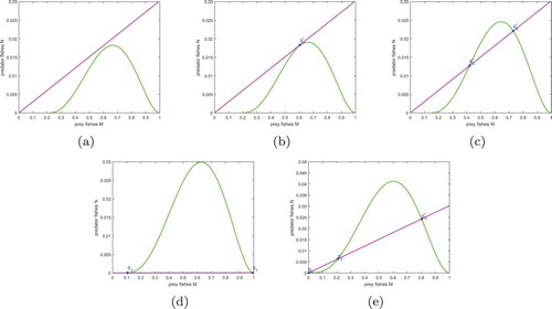
(4) ), we show the existence of non-negative equilibria in Figure . The values of parameter except β are
. Those figures are the possible number of equilibria under five different cases. The manganese violet lines represent the curves of implicit function
, and the green lines represent the curves of implicit function
. (a) When
, the two curves do not intersect at any point in the interior of the feasible domain (the green curves is below the manganese violet lines), which means that there is no positive equilibrium; (b) when
, there are two equal equilibria, that is there is only one equilibrium; (c) when
, the both curves cross twice, which means that there are two equilibriums; (d) when
and E = 480, there are two boundary equilibriums; (e) when
, there are two positive equilibriums and one extinction equilibrium.
Figure 1. The possible number of equilibria of system (Equation4(4)
(4) ) with different values of parameter β: (a)
, (b)
, (c)
, (d)
, (e)
.
2.2. The local stability of equilibria
In this section, we discuss the local stability of system (Equation4(4)
(4) ) at equilibria.
Because system (Equation4(4)
(4) ) is not linearizable about
,
and
, the local stability of them cannot be studied. In the following, we discuss the local stability of coexistence equilibria of system (Equation4
(4)
(4) ) when
.
Let be the arbitrary coexistence equilibrium, we have a linear system of system (Equation4
(4)
(4) ) at
as follows:
(8)
(8) where
,
The characteristic equation of system (Equation8
(8)
(8) ) is
(9)
(9) According to the characteristic equation (Equation9
(9)
(9) ) and the coexistence equilibrium
, we have that
, and
We know that
from
and
. Therefore, we have
,
for
, that is the positive equilibrium
is unstable.
Similarly, we have that and
exist if
from Theorem 2.1. We have that at the positive equilibrium
,
If
, then we have
which leads to that
and
. Therefore, when
, Equation (Equation9
(9)
(9) ) has two negative real part roots, that is the positive equilibrium
is locally asymptotically stable.
Similarly, when , Equation (Equation9
(9)
(9) ) has two negative real part roots if
, that is the positive equilibrium
is locally asymptotically stable.
In order to analyse the local stability of the extinction equilibrium, we redefine the variables ,
as
,
. Then system (Equation4
(4)
(4) ) transforms to the following form:
(10)
(10) Clearly, system (Equation10
(10)
(10) ) has two equilibrium points, namely the extinction equilibrium
and the coexistence equilibrium
. At the coexistence equilibrium, we have
and X satisfies
(11)
(11) Discussing the local stability of system (Equation4
(4)
(4) ) is equivalent to discussing the local stability of system (Equation10
(10)
(10) ) at the extinction equilibrium
when
. Let
be the arbitrary equilibrium of system (Equation10
(10)
(10) ), we have a linear system of system (Equation10
(10)
(10) ) at
as follows:
(12)
(12) where
,
The characteristic equation of system (Equation12
(12)
(12) ) is
(13)
(13) The characteristic equation (Equation13
(13)
(13) ) at
is
(14)
(14) From Equation (Equation14
(14)
(14) ), we can clearly see that
and
. Therefore, Equation (Equation14
(14)
(14) ) has two negative real part roots. Thus the extinction equilibrium
is always locally asymptotically stable.
The characteristic equation (Equation13(13)
(13) ) at
is
(15)
(15) If
, then Equation (Equation15
(15)
(15) ) has two negative real part roots, that is the positive equilibrium
is locally asymptotically stable.
By analysis above, we get the following results.
Theorem 2.2
If
If
In order to better show the existence and the stability of the equilibria between system (Equation4(4)
(4) ) and (Equation10
(10)
(10) ), we summarize those results shown in Tables – as follows.
Table 1. Feasibility condition for equilibria of system (Equation4(4)
(4) ).
Table 2. Stability condition for equilibria of system (Equation4(4)
(4) ).
Table 3. Feasibility condition for equilibria of system (Equation10(10)
(10) ).
Table 4. Stability condition for equilibria of system (Equation10(10)
(10) ).
3. Bifurcation analysis of system without delay
In this section, we will analyse system (Equation3(3)
(3) ) without delay and study the existence of Hopf bifurcation in one-dimensional space domain
. We will only discuss the dynamics of the coexistence equilibrium
. For convenience, we denote the coexistence equilibrium
=
.
When , system (Equation3
(3)
(3) ) becomes following diffusion equations:
(16)
(16) We denote that
is eigenvalue of
with the Neumann boundary conditions in the
. In the following discussion, we take the conversion rate γ as bifurcation parameter. Then, the linear operator of system (Equation16
(16)
(16) ) at
is
where
Based on [Citation10,Citation43], the eigenvalue of
is given by the sequence operator
, where
The corresponding characteristic equation is
(17)
(17) where
(18)
(18) From Theorem 2.1, we know that
and
when
, here
. Therefore, all eigenvalues of Equation (Equation17
(17)
(17) ) have negative real part roots. So the coexistence equilibrium
is locally asymptotic stability.
Now, we consider the situation in the condition , here
, and investigate the existence of Hopf bifurcations of system (Equation16
(16)
(16) ).
Based on [Citation43], if there exists for certain critical value
such that
and for a only pair of complex eigenvalue
near imaginary axis, which leads to
(19)
(19) then system (Equation16
(16)
(16) ) undergoes Hopf bifurcation at the
near the
. From Equation (Equation18
(18)
(18) ), we get
is equivalent to
There are finite bifurcating points
. Namely, there exists a non-negative inter
such that
is bifurcating points for
, otherwise,
is not bifurcating points for
, which is the largest integer. Thus we have that
.
Lemma 3.1
There are bifurcating points
satisfying
for any
. It is clearly that
and
for any
.
In order to illustrate that is true for all
, we give one lemma as follows.
Lemma 3.2
Suppose that , if the hypothesis
holds, where
for
. Then
holds for all
.
Now, we consider the transverse condition in (Equation19(19)
(19) ).
Lemma 3.3
Suppose that the eigenvalues near the purely imaginary are at
for
. Then, we have
Combining with the above discussion, we obtain the following conclusion.
Theorem 3.4
The periodic solutions are spatially homogeneous bifurcating from , but the periodic solutions are spatially non-homogeneous bifurcating from
for
.
Remark 3.5
The method of discussing the positive equilibria and
is similar to that of the positive equilibrium
. Thus we omit the corresponding results.
4. Hopf bifurcation and its properties of system with delay
In the following, we will study the effect of delay on system. By linearizing system (Equation3(3)
(3) ) at interior
, we obtain
(20)
(20) with
(21)
(21) where
Obviously, the characteristic equation of the linearization of (Equation20
(20)
(20) ) is equivalent to the sequence of the transcendental equation
(22)
(22) where I is the
identify matrix and
,
According to Equation (Equation22(22)
(22) ), the characteristic equations for the positive equilibrium
are the following sequence of quadratic transcendental equation:
(23)
(23) where
.
4.1. Hopf bifurcation induced by delay
In this part, we will discuss the existence of Hopf bifurcation by considering time delay as bifurcation parameter. From Theorem 2.2, the positive equilibrium of system (Equation3
(3)
(3) ) is locally asymptotically stable when
. Now, we assume that
is a root of the characteristic equation (Equation23
(23)
(23) ) when
. Since the following equation about ω is
(24)
(24) Separating real and imaginary parts, we get
(25)
(25) Then, by squaring two equations above and adding up them together, we obtain
(26)
(26) where
,
.
In order to discuss the existence of the positive roots of Equation (Equation23(23)
(23) ), we need discuss the distribution of the roots of Equation (Equation26
(26)
(26) ). Let
. Some assumptions are given as follows:
(i)
(i)
Lemma 4.1
If any one of the
If any one of the
If
From (Equation25(25)
(25) ), we have
(27)
(27) Let
be the root of Equation (Equation23
(23)
(23) ) such that
and
. Then we can get the following transversality conditions.
Lemma 4.2
Suppose . If
and
hold, then we have
when
when
Proof.
Differentiating both sides of Equation (Equation23(23)
(23) ) with corresponding to τ, we get
From (Equation27
(27)
(27) ), we have
Thus when
, we have
The proof of this lemma is completed.
From (Equation27(27)
(27) ), we get
Define
Theorem 4.3
Suppose that . The following results are true.
If the assumption
If one of the assumptions
If one of the assumption
4.2. Properties of Hopf bifurcation
In this section, we will consider the direction of the Hopf bifurcation, the stability and the period of bifurcating periodic solution of system (Equation3(3)
(3) ) by applying the centre manifold and normal form theory [Citation10,Citation38]. In reminder of this paper, we only give the main conclusions.
Let , we drop the tilde for simplification of nation. Then we transform the system (Equation3
(3)
(3) ) into the following equations:
(28)
(28) for
, and t>0. Let
Then (Equation28
(28)
(28) ) is written as an abstract equation in the space
, here
,
(29)
(29) where
and
are given by
here A, B, D defined as (Equation21
(21)
(21) ),
and
here
It is clear that the origin
is an equilibrium of (Equation28
(28)
(28) ). When
, the linear equation is
(30)
(30) which has a pair of simple purely imaginary eigenvalues
.
Next, we consider the linear functional differential equation
(31)
(31) Applying the Reisz representation theorem [Citation39], there exists
matrix-valued function
of bounded variation for
such that
In fact, we can take
where
is a Dirac delta function.
Further, we suppose that is the infinitesimal generator corresponding to (Equation31
(31)
(31) ) and
is the formal adjoint of A under the bilinear paring
(32)
(32) for
,
, where
. From the above discussion, we can know that
are the eigenvalues of
, thus
are also the eigenvalues of
.
Let and
be eigenvectors of
and
respecting to the eigenvalues
and
, respectively. We obtain
We can choose the value of
as
such that
. Thus we can computer the following quantities:
where
, and
the definition of
is the same to that in the reference [Citation38], and
Based on above analysis, the following values can be given as
(33)
(33) By computing (Equation33
(33)
(33) ), we get the following theorem.
Theorem 4.4
Properties of bifurcating periodic solutions are determined as follows.
If
If
If
5. Numerical simulation
In this section, we carry out numerical simulations to verify our theoretical results by the use of software MATLAB. Let , and most values of parameters in system (Equation3
(3)
(3) ) are mentioned in reference [Citation1],
We obtain that the coexistent equilibrium of system with
is
,
and
when
. Therefore, the coexistent equilibrium
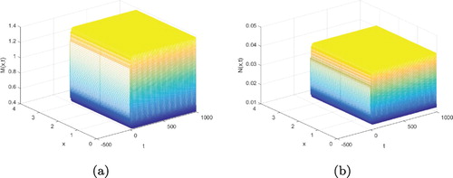
is locally asymptotically stable (see Figure ).
Figure 2. System (Equation3(3)
(3) ) at the coexistent equilibrium
is locally asymptotically stable: (a)
; (b)
.
![Figure 2. System (Equation3(3) ∂M∂t=d1ΔM+M(1−M(t−τ))(M−β)−αMN,∂N∂t=d2ΔN+γMN−δN−qEN,Mx(0,t)=Mx(π,t)=Nx(0,t)=Nx(π,t)=0,t≥0,M(x,t)=ϕ(x,t)≥0,N(x,t)=ψ(x,t)≥0,(x,t)∈[0,π]×[−τ,0],(3) ) at the coexistent equilibrium S∗ is locally asymptotically stable: (a) M(x,t); (b) N(x,t).](/cms/asset/3ab3dff0-1151-4633-89d6-0ea658394a7d/tjbd_a_1850892_f0002_oc.jpg)
From Figure , we know that is locally asymptotically stable when
. As the time increases, the prey fishes and predator fishes population fluctuate at first and then tend to be stable.
By only calculation, we obtain
Thus the critical value is
. By Theorem 3.4, system (Equation3
(3)
(3) ) is the locally asymptotically stable when
. The stability of system (Equation3
(3)
(3) ) is shown in Figure ,
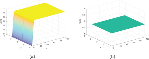
Figure 3. System (Equation3(3)
(3) ) at the coexistent equilibrium
is locally asymptotically stable when
: (a)
; (b)
.
![Figure 3. System (Equation3(3) ∂M∂t=d1ΔM+M(1−M(t−τ))(M−β)−αMN,∂N∂t=d2ΔN+γMN−δN−qEN,Mx(0,t)=Mx(π,t)=Nx(0,t)=Nx(π,t)=0,t≥0,M(x,t)=ϕ(x,t)≥0,N(x,t)=ψ(x,t)≥0,(x,t)∈[0,π]×[−τ,0],(3) ) at the coexistent equilibrium S∗ is locally asymptotically stable when τ=40<τ∗: (a) M(x,t); (b) N(x,t).](/cms/asset/8e54cfdb-8340-4ba5-9ca9-0ec377d812ad/tjbd_a_1850892_f0003_oc.jpg)
From Figure , we know that is still asymptotically stable when
. As the time increases, the prey fishes and predator fishes population first fluctuate and even tend to be stable.
Further, according to (Equation33(33)
(33) ), we obtain the values as follows:
Therefore, the periodic solutions is stable (see Figure ), Hopf-bifurcating is supercritical, and the period of the periodic solution increases.
Figure 4. The periodic solution is stable when . (a)
; (b)
.
From Figure , we chose . That is, when time delay τ increases across its critical value
, a spatially periodic solution occurs near the positive equilibrium
. However, the bifurcating periodic solution bifurcating from the critical value
may be stable on the whole phase space. A regular oscillation of the prey fishes and predator fishes population are showed.
In addition, although the local stability of the predator extinction equilibria is not given in the previous part, we can show their stability under some proper values of all parameters by numerical simulations. For example, we consider system (Equation3(3)
(3) ) with the following values:
The predator extinction equilibrium
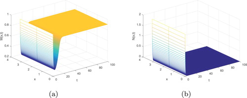
is always locally asymptotically stable, which is shown in Figure .
Figure 5. The predator extinction equilibrium is locally asymptotically stable: (a)
; (b)
.
From Figure , we can see that the number of prey fishes reaches its maximum, but the number of predator tends to zero.
Similarly, we consider system (Equation3(3)
(3) ) with the following values:
From simple computation, we obtain that
. The predator extinction equilibrium
is locally asymptotically stable, which is shown in Figure .
Figure 6. The predator extinction equilibrium is locally asymptotically stable: (a)
; (b)
.
From Figure , we can see that the number of prey fishes reaches its maximum, but the number of predator goes to zero.
6. Conclusion and discussion
Ajraldi et al. [Citation1] explained the phenomenon that the individuals of one population gather together in herds, while the other shows a more individualistic behaviour. Manna et al. [Citation15] proposed the predator–prey model considering both predator and prey with schooling behaviour. In this paper, the dynamic of a delayed diffusive predator–prey model with schooling behaviour, Allee effect and harvesting was analysed. Considering the advantage on the edge of capture of marginal predator, therefore, the relationship of them was expressed by the square root function. Meanwhile, Allee effect had been introduced in the prey intrinsic growth rate by considering the mate limitation and completion. Furthermore, we consider that fishing is an essential element in our life. We obtained that the stability of ordinary differential system around equilibria, as shown in Figures , and . From Theorem 3.4, by regarding conversion rate γ as bifurcation parameter, Hopf bifurcation of the diffusive system without time delay occurred. What's more, system (Equation3(3)
(3) ) stayed stability when the time delay
, as shown in Figure , but it lost its stability around
. Hopf-bifurcation occurred when time delay crossed its corresponding critical value, as shown in Figure . Based on normal form theory and centre manifold theorem for partial differential equations, we obtained the properties of Hopf bifurcation.
In order to make the model more practical, the time delay in maturation of predator should be considered into predator–prey model with schooling behaviour
(34)
(34) where
and
are the time delay of the resource limitation of the prey logistic equation and the time delay in maturation of predator, respectively. We leave this work in the future.
Acknowledgments
The authors are grateful to the anonymous reviewers for their constructive comments and important suggestions.
Disclosure statement
No potential conflict of interest was reported by the author(s).
Additional information
Funding
References
- V. Ajraldi, M. Pittavino, and E. Venturino, Modeling herd behavior in population systems, Nonlinear Anal.-Real. 12 (2011), pp. 2319–2338.
- W.C. Allee, Animal Aggregations: A Study in General Sociology, University of Chicago Press, Chicago, 1931.
- L. Berec, E. Angulo, and F. Courchamp, Multiple Allee effects and population management, Tre. Ecol. Evol. 22 (2007), pp. 185–191.
- S. Biswas, S.K. Sasmal, M. Saifuddin, and J. Chattopadhyay, On existence of multiple periodic solutions for Lotka-Volterra's predator-prey model with Allee effects, Nonlinear Studies 22 (2015), pp. 189–199.
- J. Brattey, Biological characteristics of atlantic cod (gadus morhua) from three inshore areas of northeastern newfoundland, Nafo Sci. Coun. Stu. 29 (1997), pp. 31–42.
- P.A. Braza, Predator-prey dynamics with square root functional responses, Nonlinear Anal.-Real. 13 (2012), pp. 1837–1843.
- E.D. Brown, J.H. Churnside, R.L. Collins, and T.S. Veenstra, Remote sensing of capelin and other biological features in the north pacific using lidar and video technology, ICES J. Mar. Sci. 59 (2002), pp. 1120–1130.
- C.W. Clark, Mathematical Bioeconomic: The Optimal Mmanagement of Renewable Resources, John Wiley. Sons., New York, 1990.
- G. Gimmelli, B.W. Kooi, and E. Venturino, Ecoepidemic models with prey group defense and feeding saturation, Ecol. Comp. 22 (2015), pp. 50–58.
- B.D. Hassard, N.D. Kazarinoff, and Y.H. Wan, Theory and Applications of Hopf Bifurcation, Cambridge University Press, Cambridge, 1981.
- D.X. Jia, T.H. Zhang, and S.L. Yuan, Pattern dynamics of a diffusive toxin producing phytoplankton-zooplankton model with three-dimensional patch, Int. J. Bifurcat. Chaos 29 (2019), pp. 1930011.
- M.A. Lewis and P. Kareiva, Allee dynamics and spread of invading organisms, Theo. Popul. Biol. 43 (1993), pp. 141–158.
- J.Z. Lin, R. Xu, and X.H. Tian, Global dynamics of an age-structured cholera model with multiple transmissions, saturation incidence and imperfect vaccination, J. Biol. Dyn. 13 (2019), pp. 69–102.
- Z.P. Ma, H.F. Huo, and H. Xiang, Spatiotemporal patterns induced by delay and cross fractional diffusion in a predator-prey model describing intraguild predation, Math. Meth. Appl. Sci. 43 (2020), pp. 5179–5196.
- D. Manna, A. Maiti, and G.P. Samanta, Analysis of a predator–prey model for exploited fish populations with schooling behavior, Appl. Math. Comput. 317 (2018), pp. 35–48.
- D. Marta, P. Bernardo, S. Attilio, and G. Tranchida, Distribution and spatial structure of pelagic fish schools in relation to the nature of the seabed in the Sicily straits (central Mediterranean), Mari. Ecol.30 (2009), pp. 151–160.
- X.Y. Meng, H.F. Huo, and X.B. Zhang, Stability and global Hopf bifurcation in a Leslie–Gower predator-prey model with stage structure for prey, J. Appl. Math. Comput. 60 (2019), pp. 1–25.
- X.Y. Meng and J. Li, Stability and Hopf bifurcation analysis of a delayed phytoplankton–zooplankton model with Allee effect and linear harvesting, Math. Biosci. Eng. 17 (2020), pp. 1973–2002.
- X.Y. Meng, N.N. Qin, and H.F. Huo, Dynamics analysis of a predator–prey system with harvesting prey and disease in prey species, J. Biol. Dynam. 12 (2018), pp. 342–374.
- X.Y. Meng and J.G. Wang, Analysis of a delayed diffusive model with Beddington–DeAngelis functional response, Int. J. Biomath.12:20191950047. (24 pages)
- X.Y. Meng and Y.Q. Wu, Bifurcation and control in a singular phytoplankton–zooplankton–fish model with nonlinear fish harvesting and taxation, Int. J. Bifurcat. Chaos. 28 (2018), pp. 1850042. (24pages)
- X.Y. Meng and Y.Q. Wu, Bifurcation analysis in a singular Beddington–Deangelis predator-prey model with two delays and nonlinear predator harvesting, Math. Biosci. Eng. 16 (2019), pp. 2668–2696.
- X.Y. Meng and Y.Q. Wu, Dynamical analysis of a fuzzy phytoplankton–zooplankton model with refuge, fishery protection and harvesting, J. Appl. Math. Comput. 63 (2020), pp. 361–389.
- O.A. Misund, J.C. Coetzee, P. Fron, and M. Gardener, Schooling behaviour of sardine Sardinops sagax in false bay, South Africa, Afr. J. Mar. Sci. 25 (2003), pp. 185–193.
- Y. Mitsunaga, C. Endo, and R.P. Babaran, Schooling behavior of juvenile yellowfin tuna Thunnus albacares around a fish aggregating device (FAD) in the Philippines, Aqua. Liv. Res. 26 (2012), pp. 79–84.
- M. Moreno and F.F. Plataniab, A cyclical square-root model for the term structure of interest rates, Eur. J. Oper. Res. 241 (2015), pp. 109–121.
- B.L. Partridge, T. Pitcher, M. Cullen, and J. Wilson, The three-dimensional structure of fish schools, Behav. Ecol. Sociobiol. 6 (1980), pp. 277–288.
- S.V. Petrovskii, A.Y. Morozov, and E. Venturino, Allee effect makes possible patchy invasion in a predator–prey system, Ecol. Lett. 5 (2002), pp. 345–352.
- S.M. Salman, A.M. Yousef, and A.A. Elsadany, Stability, bifurcation analysis and chaos control of a discrete predator–prey system with square root functional response, Chaos Solit. Fract. 93 (2016), pp. 20–31.
- G.P. Samanta, D. Manna, and A. Maiti, Bioeconomic modeling of a three-species fishery with switching effect, J. Appl. Math. Comput. 12 (2003), pp. 219–231.
- A. Szolnoki and M.c. Perc, Correlation of positive and negative reciprocity fail to confer anevolutionary: phase transitions to elementary strategies, Phys. Rev. X 3 (2013), pp. 041021. (11pages).
- X.S. Tang, H.P. Jiang, Z.Y. Deng, and T. Yu, Delay induced subcritical Hopf bifurcation in a diffusive predator–prey model with herd behavior and hyperbolic mortality, J. Appl. Anal. Comput. 7 (2017), pp. 1385–1401.
- X.Y. Tang and Y.L. Song, Stability, Hopf bifurcations and spatial patterns in a delayed diffusive predator–prey model with herd behavior, Appl. Math. Comput. 254 (2015), pp. 375–391.
- X.Y. Tang, Y.L. Song, and T.H. Zhang, Turing–Hopf bifurcation analysis of a predator–prey model with herd behavior and cross-diffusion, Nonlinear Dynam. 86 (2016), pp. 73–89.
- M.H. Wang and M. Kot, Speeds of invasion in a model with strong or weak Allee effects, Math. Biosci.171 (2001), pp. 83–97.
- J.F. Wang, J.P. Shi, and J.J. Wei, Predator–prey system with strong Allee effect in prey, J. Math. Biol. 62 (2011), pp. 291–331.
- X.C. Wang and J.J. Wei, Diffusion-driven stability and bifurcation in a predator–prey system with Ivlev-type functional response, Appl. Anal. 92 (2013), pp. 752–775.
- J.H. Wu, Theory and Applications of Partial Functional Differential Equations, Springer, New York, 1996.
- K. Yang, Delay Differential Equations with Applications in Population Dynamics, Academic Press, Boston, 1993.
- Q. Yang and H.F. Huo, Dynamics of an edge-based Seir model for sexually transmitted diseases, Math. Biosci. Eng. 17 (2020), pp. 669–699.
- R.Z. Yang, M. Liu, and C.R. Zhang, A delayed-diffusive predator-prey model with a ratio-dependent functional response, Commu. Nonlinear Sci. Num. Simul. 53 (2017), pp. 94–110.
- P. Yang, and Y.S. Wang, Hopfczero bifurcation in an age-dependent predatorcprey system with monodchaldane functional response comprising strong allee effect, J. Differ. Equations 269 (2020), pp. 9583–9618.
- F.Q. Yi, J.J. Wei, and J.P. Shi, Bifurcation and spatiotemporal patterns in a homogeneous diffusive predator–prey system, J. Differ. Equations 246 (2009), pp. 1944–1977.
- X.W. Yu, S.L. Yuan, and T.H. Zhang, Asymptotic properties of stochastic nutrient-plankton food chain models with nutrient recycling, Nonlinear Anal. Hybrid Syst. 34 (2019), pp. 209–225.
- X.B. Zhang, S.Q. Chang, and H.F. Huo, Dynamic behavior of a stochastic SIR epidemic model with vertical transmission, Electron. J. Differ. Eq. 2019 (2019), pp. 1–20.
- X.Y. Zhu, Y.X. Dai, Q.L. Li, and K. Zhao, Stability and Hopf bifurcation of a modified predator–prey model with a time delay and square root response function, Adv. Differ. Equ-Ny. 2017 (2017), pp. 235.