Survival analysis of a stochastic predator–prey model with prey refuge and fear effect

Abstract

In this paper, we propose and investigate a stochastic Holling type-II predator–prey model with prey refuge and fear effect. We first prove the existence and uniqueness of the global positive solution. Then we perform the survival analysis of the model, including the existence of a unique ergodic stationary distribution and the extinction of the model. Numerical simulations are carried out to validate our analytical results. Our findings indicate that the white noise is adverse to the growth of predator and prey populations, and the increase of fear effect will lead to the decrease of predator density, but with no obvious effect on prey density.

Keywords:

• Stochastic predator–prey model
• fear effect
• prey refuge
• stationary distribution
• extinction

MSC SUBJECT CLASSIFICATIONS:

• 60H10
• 92D25

1. Introduction

Population models, as an important part of ecology, have been extensively studied and explored for their rich dynamic behaviour with the aim to provide a theoretical guidance for the protection, development and utilization of biological resources [2,5]. Among the most important population models, predator–prey models play an important role in understanding the interaction of different species in volatile natural environments and have been widely investigated [1,4,9,12,30,33].

As is well known, it is common for predators to hunt preys in nature. However, not all preys are captured by the predators because the preys usually have refuges where they can evade the predation [10,18,27]. This indicates that a prey refuge can protect and prevent the extinction of preys, and thus, it plays an important role in the interaction between predator and prey populations. Recently, the research of the predator–prey models with prey refuges has attracted many mathematicians' attention and some interesting results have been obtained [19,23,25,32].

Notice that in most previous predator–prey models, only the direct killing of preys in the presence of predators is considered due to its obviousness in nature. But in reality, the preys may change their behaviour when the predator they faced is powerful [13,26,28]. Some studies have shown that all preys respond to the risk of predation and show all sorts of anti-predator responses, including habitat changes, foraging, vigilance and different physiological changes. Such anti-predator behaviour can reduce the long-term cost of reproduction and increase the probability of adult survival [4]. In addition, frightened preys often forage less, so their birth rate decline and they use some survival mechanisms like starvation [3].

Considering the effect of prey refuge and fear effect, in a recent paper [37], Zhang et al. proposed a predator–prey model which takes the following form: (1) $\begin{array}{rl}\frac{\mathrm{d}x}{\mathrm{d}t}& =\frac{\alpha x}{1+Ky}-b{x}^2-\frac{\text{β}(1-m)xy}{1+a(1-m)x},\\ \frac{\mathrm{d}y}{\mathrm{d}t}& =-\gamma y+\frac{c\text{β}(1-m)xy}{1+a(1-m)x},\end{array}$(1) where $x\left(t\right)$ and $y\left(t\right)$ denote, respectively, the densities of prey and predator population at time t, α is the intrinsic growth rate of prey, b is the strength of intraspecific competition of prey, γ is the death rate of the predator, c is the conversion coefficient, K refers to the level of fear and $\text{β}/a$ is the maximum number of prey eaten per predator per unit of time. All these parameters are assumed to be positive. The term $\text{β}x/\left(1+ax\right)$ represents the Holling type-II functional response, and $(1-m)x$ is the quantity of preys available to the predators, where $m\in [0,1)$ is the protection rate of the prey refuge for prey. For this model, the authors performed a detailed stability and bifurcation analysis. We refer the readers to Ref. [37] for more details.

In fact, a real ecosystem is inevitably affected by environmental noise. Therefore, the shifting environmental effects can not be neglected, which indicates that deterministic prey–predator models have limitations in predicting dynamics accurately, while stochastic models can make it [38]. Many researchers introduced random disturbances into deterministic systems to reveal the influence of environmental noise [14,16,17,22,29,31,34–36,39–41]. Ripa et al. [24] examined the impact of environmental noise on populations and presented a general theory of environmental noise in ecological food webs. Mao et al. [21] proved that the explosion of population dynamics can be suppressed by environmental Brownian noise and obtained that even a sufficiently small noise perturbation can suppress explosions in population dynamics. Hence, it is of great significance to further incorporate environmental randomness into the deterministic model (1(1) $\begin{array}{rl}\frac{\mathrm{d}x}{\mathrm{d}t}& =\frac{\alpha x}{1+Ky}-b{x}^2-\frac{\text{β}(1-m)xy}{1+a(1-m)x},\\ \frac{\mathrm{d}y}{\mathrm{d}t}& =-\gamma y+\frac{c\text{β}(1-m)xy}{1+a(1-m)x},\end{array}$(1) ). Applying the technique used in Ref. [6] to include stochastic effects, we can obtain the stochastic version of model (1(1) $\begin{array}{rl}\frac{\mathrm{d}x}{\mathrm{d}t}& =\frac{\alpha x}{1+Ky}-b{x}^2-\frac{\text{β}(1-m)xy}{1+a(1-m)x},\\ \frac{\mathrm{d}y}{\mathrm{d}t}& =-\gamma y+\frac{c\text{β}(1-m)xy}{1+a(1-m)x},\end{array}$(1) ) as follows (see the appendix for specific proof): (2) $\begin{array}{rl}\mathrm{d}x& =\left[\frac{\alpha x}{1+Ky}-b{x}^2-\frac{\text{β}(1-m)xy}{1+a(1-m)x}\right]\mathrm{d}t+{\sigma }_{1}x\mathrm{d}{B}_1\left(t\right),\\ \mathrm{d}y& =\left[-\gamma y+\frac{c\text{β}(1-m)xy}{1+a(1-m)x}\right]\mathrm{d}t+{\sigma }_{2}y\mathrm{d}{B}_2\left(t\right),\end{array}$(2) where $B_1\left(t\right)$ and $B_2\left(t\right)$ are two independent standard Brownian motions defined in a complete probability space $(\mathrm{\Omega },\mathcal{F},\{{\mathcal{F}}_t{\}}_{t\ge 0},\mathbb{P})$ with a filtration $\{{\mathcal{F}}_t{\}}_{t\ge 0}$ satisfying the usual conditions, and ${\sigma }_i^2,i=1,2$ are the intensities of the white noises. In this paper, we will devote ourselves to the investigation on the dynamics of the stochastic model (2(2) $\begin{array}{rl}\mathrm{d}x& =\left[\frac{\alpha x}{1+Ky}-b{x}^2-\frac{\text{β}(1-m)xy}{1+a(1-m)x}\right]\mathrm{d}t+{\sigma }_{1}x\mathrm{d}{B}_1\left(t\right),\\ \mathrm{d}y& =\left[-\gamma y+\frac{c\text{β}(1-m)xy}{1+a(1-m)x}\right]\mathrm{d}t+{\sigma }_{2}y\mathrm{d}{B}_2\left(t\right),\end{array}$(2) ).

The organization of this paper is as follows. In the next section, we present some necessary notations and preliminary results of model (2(2) $\begin{array}{rl}\mathrm{d}x& =\left[\frac{\alpha x}{1+Ky}-b{x}^2-\frac{\text{β}(1-m)xy}{1+a(1-m)x}\right]\mathrm{d}t+{\sigma }_{1}x\mathrm{d}{B}_1\left(t\right),\\ \mathrm{d}y& =\left[-\gamma y+\frac{c\text{β}(1-m)xy}{1+a(1-m)x}\right]\mathrm{d}t+{\sigma }_{2}y\mathrm{d}{B}_2\left(t\right),\end{array}$(2) ). In Section 3, we prove the existence of a unique ergodic stationary distribution of the model, and in Section 4, we perform the extinction analysis of the model. Some numerical simulations are carried out in Section 5 to illustrate our theoretical results. We close the paper with conclusion in Section 6.

2. Preliminaries

In this section, we present some notations and basic results about model (2(2) $\begin{array}{rl}\mathrm{d}x& =\left[\frac{\alpha x}{1+Ky}-b{x}^2-\frac{\text{β}(1-m)xy}{1+a(1-m)x}\right]\mathrm{d}t+{\sigma }_{1}x\mathrm{d}{B}_1\left(t\right),\\ \mathrm{d}y& =\left[-\gamma y+\frac{c\text{β}(1-m)xy}{1+a(1-m)x}\right]\mathrm{d}t+{\sigma }_{2}y\mathrm{d}{B}_2\left(t\right),\end{array}$(2) ), which are the basis for further investigation on the dynamics of model (2(2) $\begin{array}{rl}\mathrm{d}x& =\left[\frac{\alpha x}{1+Ky}-b{x}^2-\frac{\text{β}(1-m)xy}{1+a(1-m)x}\right]\mathrm{d}t+{\sigma }_{1}x\mathrm{d}{B}_1\left(t\right),\\ \mathrm{d}y& =\left[-\gamma y+\frac{c\text{β}(1-m)xy}{1+a(1-m)x}\right]\mathrm{d}t+{\sigma }_{2}y\mathrm{d}{B}_2\left(t\right),\end{array}$(2) ).

Consider the following n-dimensional stochastic differential equation: (3) $\mathrm{d}x\left(t\right)=f\left(x\right(t),t)\mathrm{d}t+g\left(x\right(t),t)\mathrm{d}B\left(t\right)\mathrm{f}\mathrm{o}\mathrm{r}t\ge t_0.$(3) Denote by $C^{2,1}({\mathbb{R}}^n\times [t_0,\mathrm{\infty });{\mathbb{R}}_{+})$ the family of all nonnegative functions $V(x,t)$ defined on ${\mathbb{R}}^n\times [t_0,\mathrm{\infty })$ such that they are continuously twice differentiable in x and once in t. We introduce the differential operator defined in Ref. [20] $L=\frac{\mathrm{\partial }}{\mathrm{\partial }t}+\sum _{i=1}^n{f}_i(x,t)\frac{\mathrm{\partial }}{\mathrm{\partial }{x}_i}+\frac{1}{2}\sum _{i,j=1}^n\left[g^T\right(x,t\left)g\right(x,t){]}_{ij}\frac{{\mathrm{\partial }}^2}{\mathrm{\partial }{x}_i\mathrm{\partial }{x}_j}.$If L acts on a function $V\in C^{2,1}({\mathbb{R}}^n\times [t_0,\mathrm{\infty });{\mathbb{R}}_{+}),$ then $LV(x,t)=V_t(x,t)+V_x(x,t)f(x,t)+\frac{1}{2}\mathrm{t}\mathrm{r}\mathrm{a}\mathrm{c}\mathrm{e}\left[g^T\right(x,t\left)V_{xx}\right(x,t\left)g\right(x,t\left)\right],$where $V_t=\mathrm{\partial }V/\mathrm{\partial }t,V_x=(\mathrm{\partial }V/\mathrm{\partial }{x}_1,\dots ,\mathrm{\partial }V/\mathrm{\partial }{x}_n)$ and $V_{xx}=({\mathrm{\partial }}^{2}V/\mathrm{\partial }{x}_i\mathrm{\partial }{x}_j{)}_{n\times n}$. From Itô's formula, if $x\left(t\right)\in {\mathbb{R}}^n$, then $\mathrm{d}V\left(x\right(t),t)=LV\left(x\right(t),t)\mathrm{d}t+V_x\left(x\right(t),t)g\left(x\right(t),t)\mathrm{d}B\left(t\right).$The following theorem is about the existence and uniqueness of the global positive solution of model (2(2) $\begin{array}{rl}\mathrm{d}x& =\left[\frac{\alpha x}{1+Ky}-b{x}^2-\frac{\text{β}(1-m)xy}{1+a(1-m)x}\right]\mathrm{d}t+{\sigma }_{1}x\mathrm{d}{B}_1\left(t\right),\\ \mathrm{d}y& =\left[-\gamma y+\frac{c\text{β}(1-m)xy}{1+a(1-m)x}\right]\mathrm{d}t+{\sigma }_{2}y\mathrm{d}{B}_2\left(t\right),\end{array}$(2) ).

Theorem 2.1

For any given initial value $\left(x\right(0),y(0\left)\right)\in {\mathbb{R}}_{+}^2$, there exists a unique solution $\left(x\right(t),y(t\left)\right)$ of model (2(2) $\begin{array}{rl}\mathrm{d}x& =\left[\frac{\alpha x}{1+Ky}-b{x}^2-\frac{\text{β}(1-m)xy}{1+a(1-m)x}\right]\mathrm{d}t+{\sigma }_{1}x\mathrm{d}{B}_1\left(t\right),\\ \mathrm{d}y& =\left[-\gamma y+\frac{c\text{β}(1-m)xy}{1+a(1-m)x}\right]\mathrm{d}t+{\sigma }_{2}y\mathrm{d}{B}_2\left(t\right),\end{array}$(2) ) on $t\ge 0$ and the solution will remain in ${\mathbb{R}}_{+}^2$ with probability one, that is to say, $\left(x\right(t),y(t\left)\right)\in {\mathbb{R}}_{+}^2$ for all $t\ge 0$ almost surely (a.s.).

Proof.

Since the coefficients of model (2(2) $\begin{array}{rl}\mathrm{d}x& =\left[\frac{\alpha x}{1+Ky}-b{x}^2-\frac{\text{β}(1-m)xy}{1+a(1-m)x}\right]\mathrm{d}t+{\sigma }_{1}x\mathrm{d}{B}_1\left(t\right),\\ \mathrm{d}y& =\left[-\gamma y+\frac{c\text{β}(1-m)xy}{1+a(1-m)x}\right]\mathrm{d}t+{\sigma }_{2}y\mathrm{d}{B}_2\left(t\right),\end{array}$(2) ) satisfy the local Lipschitz condition, then there exists a unique local solution $\left(x\right(t),y(t\left)\right)$ of model (2(2) $\begin{array}{rl}\mathrm{d}x& =\left[\frac{\alpha x}{1+Ky}-b{x}^2-\frac{\text{β}(1-m)xy}{1+a(1-m)x}\right]\mathrm{d}t+{\sigma }_{1}x\mathrm{d}{B}_1\left(t\right),\\ \mathrm{d}y& =\left[-\gamma y+\frac{c\text{β}(1-m)xy}{1+a(1-m)x}\right]\mathrm{d}t+{\sigma }_{2}y\mathrm{d}{B}_2\left(t\right),\end{array}$(2) ) on $t\in [0,{\tau }_e)$, a.s., where ${\tau }_e$ denotes the explosion time. To show that this solution is global, we only need to prove ${\tau }_e=\mathrm{\infty }$, a.s. Let $k_0>0$ be sufficiently large such that both $x\left(0\right)$ and $y\left(0\right)$ lie within the interval $[1/k_0,k_0]$. For each integer $k\ge k_0$, define the stopping time ${\tau }_k=inf\{t\in [0,{\tau }_e):min\left\{x\right(t),y(t\left)\right\}\le \frac{1}{k},\mathrm{o}\mathrm{r}max\left\{x\right(t),y(t\left)\right\}\ge k\},$where ${\tau }_k$ is increasing as $k\to \mathrm{\infty }$. Set ${\tau }_{\mathrm{\infty }}=\underset{k\to \mathrm{\infty }}{lim}{\tau }_k$, which implies ${\tau }_{\mathrm{\infty }}\le {\tau }_e$, a.s. Hence to complete the proof, we only need to show that ${\tau }_{\mathrm{\infty }}=\mathrm{\infty }$, a.s. We prove this by contradiction. If ${\tau }_{\mathrm{\infty }}<\mathrm{\infty }$, then there exist a pair of constants $ϵ\in (0,1)$ and T>0 such that $P({\tau }_{\mathrm{\infty }}<T)>ϵ.$Therefore, there exists $k_1\ge k_0$ such that for all $k\ge k_1$, $P\left({\mathrm{\Omega }}_k\right)\ge ϵ,$where ${\mathrm{\Omega }}_k=\{{\tau }_k\le T\}$. Then define a $C^2$-function V: ${\mathbb{R}}_{+}^2\to {\mathbb{R}}_{\mathbb{+}}$ by $V=x-\frac{\gamma }{2c\text{β}(1-m)}-\frac{\gamma }{2c\text{β}(1-m)}\ln \frac{2c\text{β}(1-m)x}{\gamma }+\frac{1}{c}(y-1-\ln y).$From Itô's formula, (4) $\mathrm{d}V(x,y)=LV(x,y)\mathrm{d}t+\left[{\sigma }_{1}x-\frac{\gamma {\sigma }_1}{2c\text{β}(1-m)}\right]\mathrm{d}{B}_1\left(t\right)+\left(\frac{{\sigma }_{2}y}{c}-\frac{{\sigma }_2}{c}\right)\mathrm{d}{B}_2\left(t\right),$(4) where $\begin{array}{rl}LV(x,y)& =\frac{\alpha x}{1+Ky}-b{x}^2-\frac{\text{β}(1-m)xy}{1+a(1-m)x}-\frac{\alpha \gamma }{2c\text{β}(1-m)(1+Ky)}+\frac{b\gamma x}{2c\text{β}(1-m)}\\ & +\frac{\gamma }{2c}\frac{y}{1+a(1-m)x}+\frac{\gamma {\sigma }_1^2}{4c\text{β}(1-m)}-\frac{\gamma }{c}y+\frac{\text{β}(1-m)xy}{1+a(1-m)x}+\frac{\gamma }{c}\\ & -\frac{\text{β}(1-m)x}{1+a(1-m)x}+\frac{{\sigma }_2^2}{2c}\\ & \le \alpha x-b{x}^2+\frac{b\gamma x}{2c\text{β}(1-m)}+\frac{\gamma }{2c}y+\frac{\gamma {\sigma }_1^2}{4c\text{β}(1-m)}-\frac{\gamma }{c}y+\frac{\gamma }{c}+\frac{{\sigma }_2^2}{2c}\\ & \le -b{x}^2+\left[\alpha +\frac{b\gamma }{2c\text{β}(1-m)}\right]x-\frac{\gamma }{2c}y+\frac{\gamma {\sigma }_1^2}{4c\text{β}(1-m)}+\frac{\gamma }{c}+\frac{{\sigma }_2^2}{2c}\\ & \le \frac{\gamma {\sigma }_1^2}{4c\text{β}(1-m)}+\frac{\gamma }{c}+\frac{{\sigma }_2^2}{2c}+\tilde{J}:=J.\end{array}$Here, $\tilde{J}=\underset{(x,y)\in (0,\mathrm{\infty })}{sup}\{-b{x}^2+\left[\alpha +\frac{b\gamma }{2c\text{β}(1-m)}\right]x-\frac{\gamma }{2c}y\}.$Integrating and taking the expectation of both sides of (4(4) $\mathrm{d}V(x,y)=LV(x,y)\mathrm{d}t+\left[{\sigma }_{1}x-\frac{\gamma {\sigma }_1}{2c\text{β}(1-m)}\right]\mathrm{d}{B}_1\left(t\right)+\left(\frac{{\sigma }_{2}y}{c}-\frac{{\sigma }_2}{c}\right)\mathrm{d}{B}_2\left(t\right),$(4) ) from 0 to ${\tau }_k\wedge T$, we obtain (5) $EV\left(x\left({\tau }_k\wedge T\right),y\left({\tau }_k\wedge T\right)\right)\le V\left(x\left(0\right),y\left(0\right)\right)+JE\left({\tau }_k\wedge T\right)\le V\left(x\left(0\right),y\left(0\right)\right)+JT.$(5) Noting that for every $\omega \in {\mathrm{\Omega }}_k$, $x({\tau }_k,\omega )$ or $y({\tau }_k,\omega )$ equals either k or $1/k$. Hence $\begin{array}{rl}V\left(x\left({\tau }_k\right),y\left({\tau }_k\right)\right)& \ge \left[k-\frac{\gamma }{2c\text{β}(1-m)}-\frac{\gamma }{2c\text{β}(1-m)}\ln \frac{2c\text{β}(1-m)k}{\gamma }\right]\\ & \wedge \left[\frac{1}{k}-\frac{\gamma }{2c\text{β}(1-m)}-\frac{\gamma }{2c\text{β}(1-m)}\ln \frac{2c\text{β}(1-m)}{\gamma k}\right]\\ & \wedge \left[\frac{1}{c}(k-1-\ln k)\right]\wedge \left[\frac{1}{c}\left(\frac{1}{k}-1+\ln k\right)\right].\end{array}$From (5(5) $EV\left(x\left({\tau }_k\wedge T\right),y\left({\tau }_k\wedge T\right)\right)\le V\left(x\left(0\right),y\left(0\right)\right)+JE\left({\tau }_k\wedge T\right)\le V\left(x\left(0\right),y\left(0\right)\right)+JT.$(5) ), we have $\begin{array}{rl}V\left(x\left(0\right),y\left(0\right)\right)+JT& \ge E\left(I_{{\mathrm{\Omega }}_k}V\left(x\left({\tau }_k\right),y\left({\tau }_k\right)\right)\right)\\ & \ge ϵ\{\left[k-\frac{\gamma }{2c\text{β}(1-m)}-\frac{\gamma }{2c\text{β}(1-m)}\ln \frac{2c\text{β}(1-m)k}{\gamma }\right]\\ & \wedge \left[\frac{1}{k}-\frac{\gamma }{2c\text{β}(1-m)}-\frac{\gamma }{2c\text{β}(1-m)}\ln \frac{2c\text{β}(1-m)}{\gamma k}\right]\\ & \wedge \left[\frac{1}{c}(k-1-\ln k)\right]\wedge \left[\frac{1}{c}\left(\frac{1}{k}-1+\ln k\right)\right]\}.\end{array}$This leads to a contradiction as we let $k\to \mathrm{\infty }$, $\mathrm{\infty }>V\left(x\left(0\right),y\left(0\right)\right)+JT=\mathrm{\infty }.$So we have that ${\tau }_{\mathrm{\infty }}=\mathrm{\infty }$, a.s.

Next, we present a lemma which gives a condition for the existence of a unique ergodic stationary distribution of system (3(3) $\mathrm{d}x\left(t\right)=f\left(x\right(t),t)\mathrm{d}t+g\left(x\right(t),t)\mathrm{d}B\left(t\right)\mathrm{f}\mathrm{o}\mathrm{r}t\ge t_0.$(3) ). Let $X\left(t\right)$ be a homogeneous Markov process in ${\mathbb{R}}^n$ described by the following stochastic differential equation: $\mathrm{d}X\left(t\right)=b\left(X\right)\mathrm{d}t+\sum _{r=1}^k{g}_r\left(X\right)\mathrm{d}{B}_r\left(t\right),$and the diffusion matrix is $A\left(x\right)=\left(a_{ij}\right(x\left)\right),a_{ij}\left(x\right)=\sum _{r=1}^k{g}_r^i\left(x\right)g_r^j\left(x\right).$

Lemma 2.2

[7]

The Markov process $X\left(t\right)$ has a unique ergodic stationary distribution $\mu (\cdot )$, if there exists a bounded domain $D\subset {\mathbb{R}}^n$ with regular boundary Γ and

• there is a positive number M such that $\sum _{i,j=1}^n{a}_{ij}\left(x\right){\xi }_i{\xi }_j\ge M{\left|\xi \right|}^2,x\in D,\xi \in {\mathbb{R}}^n.$

• There exists a nonnegative $C^2-$ function V such that LV is negative for any ${\mathbb{R}}^n\mathrm{\setminus }D$. Then $P\left\{\underset{T\to \mathrm{\infty }}{lim}\frac{1}{T}{\int }_0^{T}f\left(X\left(t\right)\right)\mathrm{d}t={\int }_{{\mathbb{R}}^n}f\left(x\right)\mu \left(\mathrm{d}x\right)\right\}=1$for all $x\in {\mathbb{R}}^n$, where $f(\cdot )$ is a function integrable with respect to the measure μ.

3. Stationary distribution

In this section, we establish sufficient conditions for the existence of a unique ergodic stationary distribution. First, we give the following assumptions:

(H1)

$\gamma >\frac{1}{2}max\{{\sigma }_1^2,{\sigma }_2^2\}$;

(H2)

$\lambda =\frac{2\alpha c\text{β}(1-m)}{b+2a\alpha (1-m)}-\frac{2\alpha c\text{β}(1-m)}{3b[1+a(1-m\left)\right(2\alpha /b){]}^2}-\frac{4c_2{\alpha }^2}{3b}-\frac{c_2\alpha {\sigma }_1^2}{2b}-\gamma -\frac{{\sigma }_2^2}{2}>0$, where $c_2$ is a positive constant satisfying that (6) $c_2>\frac{3c\text{β}a(1-m{)}^2}{b{\left[1+a(1-m)\frac{2\alpha }{b}\right]}^3}+\frac{c\text{β}(1-m)}{\alpha {\left[1+a(1-m)\frac{2\alpha }{b}\right]}^2}.$(6)

Theorem 3.1

Let $\left(x\right(t),y(t\left)\right)$ be the solution of model (2(2) $\begin{array}{rl}\mathrm{d}x& =\left[\frac{\alpha x}{1+Ky}-b{x}^2-\frac{\text{β}(1-m)xy}{1+a(1-m)x}\right]\mathrm{d}t+{\sigma }_{1}x\mathrm{d}{B}_1\left(t\right),\\ \mathrm{d}y& =\left[-\gamma y+\frac{c\text{β}(1-m)xy}{1+a(1-m)x}\right]\mathrm{d}t+{\sigma }_{2}y\mathrm{d}{B}_2\left(t\right),\end{array}$(2) ) with any given initial value $\left(x\right(0),y(0\left)\right)\in {\mathbb{R}}_{+}^2$. If assumptions ($H_1$) and $\left(H_2\right)$ are satisfied, then model (2(2) $\begin{array}{rl}\mathrm{d}x& =\left[\frac{\alpha x}{1+Ky}-b{x}^2-\frac{\text{β}(1-m)xy}{1+a(1-m)x}\right]\mathrm{d}t+{\sigma }_{1}x\mathrm{d}{B}_1\left(t\right),\\ \mathrm{d}y& =\left[-\gamma y+\frac{c\text{β}(1-m)xy}{1+a(1-m)x}\right]\mathrm{d}t+{\sigma }_{2}y\mathrm{d}{B}_2\left(t\right),\end{array}$(2) ) admits a unique stationary distribution $\mu (\cdot )$ and it has the ergodic property.

Proof.

By the condition (B.2) in Lemma 2.2, we need to construct a $C^2$-continuous function $V:{\mathbb{R}}_{+}^2\to {\mathbb{R}}_{+}$ and a bounded closed $U_{ϵ}$ such that $LV\le -1$ for $(x,y)\in {\mathbb{R}}_{+}^2\mathrm{\setminus }{U}_{ϵ}$. To this end, let ${\sigma }_{max}=max\{{\sigma }_1,{\sigma }_2\}$ and choose a constant $\theta >0$ such that $\rho =\gamma -\left(1/2\right){\sigma }_{max}^2(\theta +1)>0$, and define a $C^2$-function $\tilde{V}:{\mathbb{R}}_{+}^2\to \mathbb{R}$ as follows: $\tilde{V}=M\left[-c_{1}x+c_2\left(x-\frac{\alpha }{b}\ln x\right)+\frac{c_2\text{β}(1-m)\alpha }{b\gamma }y-\ln y\right]+\frac{1}{\theta +2}{\left(x+\frac{y}{c}\right)}^{\theta +2},$where $c_1=\left(c\text{β}\right(1-m\left)\right)/\left(3\alpha \right[1+a(1-m)\left(2\alpha /b\right){]}^2)+(2/3)c_2$ and $c_2$ is defined in (6(6) $c_2>\frac{3c\text{β}a(1-m{)}^2}{b{\left[1+a(1-m)\frac{2\alpha }{b}\right]}^3}+\frac{c\text{β}(1-m)}{\alpha {\left[1+a(1-m)\frac{2\alpha }{b}\right]}^2}.$(6) ) (obviously, condition (6(6) $c_2>\frac{3c\text{β}a(1-m{)}^2}{b{\left[1+a(1-m)\frac{2\alpha }{b}\right]}^3}+\frac{c\text{β}(1-m)}{\alpha {\left[1+a(1-m)\frac{2\alpha }{b}\right]}^2}.$(6) ) implies that $c_2>c_1$); $M=\left(2/\lambda \right)max\{2,R_1\}$ and $R_1$ is to be determined later. We can easily check that $\underset{ϵ\to 0,(x,y)\in {\mathbb{R}}_{+}^2\mathrm{\setminus }{U}_{ϵ}}{lim inf}\tilde{V}(x,y)=\mathrm{\infty },$where $U_{ϵ}:=(ϵ,1/ϵ)\times (ϵ,1/ϵ)$, and $ϵ>0$ is a sufficiently small number. Notice that $\tilde{V}(x,y)$ has a global minimum point $(x_0,y_0)$ in the interior of ${\mathbb{R}}_{+}^2$. Then, we can define a nonnegative $C^2$-function $V:{\mathbb{R}}_{+}^2\to {\mathbb{R}}_{+}$ by (7) $V(x,y)=\tilde{V}(x,y)-\tilde{V}(x_0,y_0)=M{V}_1(x,y)+V_2(x,y),$(7) where $\begin{array}{rl}{V}_1(x,y)& =-c_{1}x+c_2\left(x-\frac{\alpha }{b}\ln x\right)+\frac{c_2\text{β}(1-m)\alpha }{b\gamma }y-\ln y,\\ V_2(x,y)& =\frac{1}{\theta +2}{\left(x+\frac{y}{c}\right)}^{\theta +2}-\tilde{V}(x_0,y_0).\end{array}$Applying Itô's formula to $V_1(x,y)$, we have $\begin{array}{rl}L{V}_1& =-\frac{c_1\alpha x}{1+Ky}+c_{1}b{x}^2+\frac{c_1\text{β}(1-m)xy}{1+a(1-m)x}+\frac{c_2\alpha x}{1+Ky}-c_{2}b{x}^2-\frac{c_2\text{β}(1-m)xy}{1+a(1-m)x}\\ & -\frac{c_2{\alpha }^2}{b(1+Ky)}+c_2\alpha x+\frac{c_2\alpha \text{β}(1-m)y}{b[1+a(1-m\left)x\right]}+\frac{c_2\alpha {\sigma }_1^2}{2b}-\frac{c_2\text{β}(1-m)\alpha }{b}y\\ & +\frac{c_{2}c{\text{β}}^2(1-m{)}^2\alpha xy}{b\gamma [1+a(1-m\left)x\right]}+\gamma -\frac{c\text{β}(1-m)x}{1+a(1-m)x}+\frac{{\sigma }_2^2}{2}\\ & \le \frac{\alpha (c_2-c_1)x}{1+Ky}+c_{1}b{x}^2+c_1\text{β}(1-m)xy-c_{2}b{x}^2+c_2\alpha x+\frac{c_2\alpha \text{β}(1-m)}{b}y+\frac{c_2\alpha {\sigma }_1^2}{2b}\\ & -\frac{c_2\alpha \text{β}(1-m)}{b}y+\frac{c_{2}c{\text{β}}^2(1-m{)}^2\alpha xy}{b\gamma }+\gamma -\frac{c\text{β}(1-m)x}{1+a(1-m)x}+\frac{{\sigma }_2^2}{2}\\ & \le c_2\alpha x-c_1\alpha x+c_{1}b{x}^2-c_{2}b{x}^2+c_2\alpha x-\frac{c\text{β}(1-m)x}{1+a(1-m)x}\\ & +[c_1\text{β}(1-m)+\frac{c_{2}c{\text{β}}^2(1-m{)}^2\alpha }{b\gamma }]xy+\frac{c_2\alpha {\sigma }_1^2}{2b}+\gamma +\frac{{\sigma }_2^2}{2}\\ & =c_2\alpha x\left(2-\frac{b}{\alpha }x\right)+c_1\alpha \left[x\left(\frac{b}{\alpha }x-1\right)-\frac{2\alpha }{b}\right]-\frac{c\text{β}(1-m)x}{1+a(1-m)x}\\ & +[c_1\text{β}(1-m)+\frac{c_{2}c{\text{β}}^2(1-m{)}^2\alpha }{b\gamma }]xy+\frac{2c_1{\alpha }^2}{b}+\frac{c_2\alpha {\sigma }_1^2}{2b}+\gamma +\frac{{\sigma }_2^2}{2}\\ & =-\frac{c\text{β}(1-m)\left(2\alpha /b\right)}{1+a(1-m)\left(2\alpha /b\right)}+\frac{2c_1{\alpha }^2}{b}+\frac{c_2\alpha {\sigma }_1^2}{2b}+\gamma +\frac{{\sigma }_2^2}{2}+\{-\frac{c\text{β}(1-m)x}{1+a(1-m)x}\\ & +\frac{c\text{β}(1-m)\left(2\alpha /b\right)}{1+a(1-m)\left(2\alpha /b\right)}+c_2\alpha x\left(2-\frac{b}{\alpha }x\right)+c_1\alpha \left[x\left(\frac{b}{\alpha }x-1\right)-\frac{2\alpha }{b}\right]\}\\ & +\left[c_1\text{β}(1-m)+\frac{c_{2}c{\text{β}}^2(1-m{)}^2\alpha }{b\gamma }\right]xy\\ & =-\frac{c\text{β}(1-m)\left(2\alpha /b\right)}{1+a(1-m)\left(2\alpha /b\right)}+\frac{2c_1{\alpha }^2}{b}+\frac{c_2\alpha {\sigma }_1^2}{2b}+\gamma +\frac{{\sigma }_2^2}{2}\\ & +[c_1\text{β}(1-m)+\frac{c_{2}c{\text{β}}^2(1-m{)}^2\alpha }{b\gamma }]xy+F\left(x\right),\end{array}$where $\begin{array}{rl}F\left(x\right)& =-\frac{c\text{β}(1-m)x}{1+a(1-m)x}+\frac{c\text{β}(1-m)\left(2\alpha /b\right)}{1+a(1-m)\left(2\alpha /b\right)}+c_2\alpha x\left(2-\frac{b}{\alpha }x\right)\\ & +c_1\alpha \left[x\left(\frac{b}{\alpha }x-1\right)-\frac{2\alpha }{b}\right].\end{array}$We can compute that $F^{\mathrm{\prime }}\left(x\right)=-\frac{c\text{β}(1-m)}{[1+a(1-m)x{]}^2}+2c_2\alpha -2c_{2}bx+2c_{1}bx-c_1\alpha$and $F^{\mathrm{\prime }\mathrm{\prime }}\left(x\right)=\frac{2c\text{β}a(1-m{)}^2}{[1+a(1-m)x{]}^3}-2c_{2}b+2c_{1}b.$Therefore, $F^{\mathrm{\prime }}\left(x\right){|}_{x=2\alpha /b}=-\frac{c\text{β}(1-m)}{{\left[1+a(1-m)\left(2\alpha /b\right)\right]}^2}-2c_2\alpha +3c_1\alpha =0,$due to the equality $c_1=\left(c\text{β}\right(1-m\left)\right)/\left(3\alpha \right[1+a(1-m)\left(2\alpha /b\right){]}^2)+(2/3)c_2$. Moreover, we can compute that $F^{\mathrm{\prime }\mathrm{\prime }}\left(x\right){|}_{x=2\alpha /b}=\frac{2c\text{β}a(1-m{)}^2}{{\left[1+a(1-m)\left(2\alpha /b\right)\right]}^3}-2c_{2}b+2c_{1}b<0,$where we have used inequality (6(6) $c_2>\frac{3c\text{β}a(1-m{)}^2}{b{\left[1+a(1-m)\frac{2\alpha }{b}\right]}^3}+\frac{c\text{β}(1-m)}{\alpha {\left[1+a(1-m)\frac{2\alpha }{b}\right]}^2}.$(6) ). Hence, we have that for all $x\in {\mathbb{R}}_{+}$, $F\left(x\right)\le F\left(\frac{2\alpha }{b}\right)=0.$Consequently, (8) $\begin{array}{rl}L{V}_1& \le -\frac{c\text{β}(1-m)\left(2\alpha /b\right)}{1+a(1-m)\left(2\alpha /b\right)}+\frac{2c_1{\alpha }^2}{b}+\frac{c_2\alpha {\sigma }_1^2}{2b}+\gamma +\frac{{\sigma }_2^2}{2}\\ & +[c_1\text{β}(1-m)+\frac{c_{2}c{\text{β}}^2(1-m{)}^2\alpha }{b\gamma }]xy\\ & =-\frac{c\text{β}(1-m)\left(2\alpha /b\right)}{1+a(1-m)\left(2\alpha /b\right)}+\frac{2\alpha c\text{β}(1-m)}{3b{\left[1+a(1-m)\left(2\alpha /b\right)\right]}^2}\\ & +\frac{4c_2{\alpha }^2}{3b}+\frac{c_2\alpha {\sigma }_1^2}{2b}+\gamma +\frac{{\sigma }_2^2}{2}\\ & +\left[c_1\text{β}(1-m)+\frac{c_{2}c{\text{β}}^2(1-m{)}^2\alpha }{b\gamma }\right]xy\\ & :=-\lambda +\left[c_1\text{β}(1-m)+\frac{c_{2}c{\text{β}}^2(1-m{)}^2\alpha }{b\gamma }\right]xy,\end{array}$(8) where λ is a positive number defined in assumption ($H_2$).

Similarly, we can compute that (9) $\begin{array}{rl}L{V}_2& ={\left(x+\frac{y}{c}\right)}^{\theta +1}\left[\frac{\alpha x}{1+Ky}-b{x}^2-\frac{\text{β}(1-m)xy}{1+a(1-m)x}-\frac{\gamma }{c}y+\frac{\text{β}(1-m)xy}{1+a(1-m)x}\right]\\ & +\frac{1}{2}(\theta +1){\left(x+\frac{y}{c}\right)}^{\theta }\left[{\sigma }_1^2{x}^2+{\sigma }_2^2{\left(\frac{y}{c}\right)}^2\right]\\ & \le {\left(x+\frac{y}{c}\right)}^{\theta +1}\left[(\alpha +\gamma )x-b{x}^2-\gamma x-\frac{\gamma }{c}y\right]\\ & +\frac{1}{2}(\theta +1){\left(x+\frac{y}{c}\right)}^{\theta }\left[{\sigma }_1^2{x}^2+{\sigma }_2^2{\left(\frac{y}{c}\right)}^2\right]\\ & \le {\left(x+\frac{y}{c}\right)}^{\theta +1}\left[G-\gamma \left(x+\frac{y}{c}\right)\right]+\frac{1}{2}{\sigma }_{max}^2(\theta +1){\left(x+\frac{y}{c}\right)}^{\theta +2}\\ & =G{\left(x+\frac{y}{c}\right)}^{\theta +1}-\gamma {\left(x+\frac{y}{c}\right)}^{\theta +2}+\frac{1}{2}{\sigma }_{max}^2(\theta +1){\left(x+\frac{y}{c}\right)}^{\theta +2}\\ & =G{\left(x+\frac{y}{c}\right)}^{\theta +1}-\left[\gamma -\frac{1}{2}{\sigma }_{max}^2(\theta +1)\right]{\left(x+\frac{y}{c}\right)}^{\theta +2}\\ & \le F-\frac{\rho }{2}{\left(x+\frac{y}{c}\right)}^{\theta +2}\\ & \le F-\frac{\rho }{2}\left[x^{\theta +2}+{\left(\frac{y}{c}\right)}^{\theta +2}\right],\end{array}$(9) where $\begin{array}{rl}G& =\underset{(x,y)\in {\mathbb{R}}_{+}^2}{sup}\left\{\right(\alpha +\gamma )x-b{x}^2\}<\mathrm{\infty },\\ F& =\underset{(x,y)\in {\mathbb{R}}_{+}^2}{sup}\{G{\left(x+\frac{y}{c}\right)}^{\theta +1}-\frac{\rho }{2}{\left(x+\frac{y}{c}\right)}^{\theta +2}\}<\mathrm{\infty }.\end{array}$From (7(7) $V(x,y)=\tilde{V}(x,y)-\tilde{V}(x_0,y_0)=M{V}_1(x,y)+V_2(x,y),$(7) )–(9(9) $\begin{array}{rl}L{V}_2& ={\left(x+\frac{y}{c}\right)}^{\theta +1}\left[\frac{\alpha x}{1+Ky}-b{x}^2-\frac{\text{β}(1-m)xy}{1+a(1-m)x}-\frac{\gamma }{c}y+\frac{\text{β}(1-m)xy}{1+a(1-m)x}\right]\\ & +\frac{1}{2}(\theta +1){\left(x+\frac{y}{c}\right)}^{\theta }\left[{\sigma }_1^2{x}^2+{\sigma }_2^2{\left(\frac{y}{c}\right)}^2\right]\\ & \le {\left(x+\frac{y}{c}\right)}^{\theta +1}\left[(\alpha +\gamma )x-b{x}^2-\gamma x-\frac{\gamma }{c}y\right]\\ & +\frac{1}{2}(\theta +1){\left(x+\frac{y}{c}\right)}^{\theta }\left[{\sigma }_1^2{x}^2+{\sigma }_2^2{\left(\frac{y}{c}\right)}^2\right]\\ & \le {\left(x+\frac{y}{c}\right)}^{\theta +1}\left[G-\gamma \left(x+\frac{y}{c}\right)\right]+\frac{1}{2}{\sigma }_{max}^2(\theta +1){\left(x+\frac{y}{c}\right)}^{\theta +2}\\ & =G{\left(x+\frac{y}{c}\right)}^{\theta +1}-\gamma {\left(x+\frac{y}{c}\right)}^{\theta +2}+\frac{1}{2}{\sigma }_{max}^2(\theta +1){\left(x+\frac{y}{c}\right)}^{\theta +2}\\ & =G{\left(x+\frac{y}{c}\right)}^{\theta +1}-\left[\gamma -\frac{1}{2}{\sigma }_{max}^2(\theta +1)\right]{\left(x+\frac{y}{c}\right)}^{\theta +2}\\ & \le F-\frac{\rho }{2}{\left(x+\frac{y}{c}\right)}^{\theta +2}\\ & \le F-\frac{\rho }{2}\left[x^{\theta +2}+{\left(\frac{y}{c}\right)}^{\theta +2}\right],\end{array}$(9) ), we have that (10) $\begin{array}{rl}LV& =L(V_1+V_2)\le M\{-\lambda +\left[c_1\text{β}(1-m)+\frac{c_{2}c{\text{β}}^2(1-m{)}^2\alpha }{b\gamma }\right]xy\}\\ & -\frac{\rho }{2}\left[x^{\theta +2}+{\left(\frac{y}{c}\right)}^{\theta +2}\right]+F.\end{array}$(10) Next, we prove $LV\le -1$ on ${\mathbb{R}}_{+}^2\mathrm{\setminus }{U}_{ϵ}$. Take $ϵ>0$ sufficiently small such that the following inequalities hold: (11) $\begin{array}{rl}& 0<ϵ<\frac{\lambda b\gamma }{4\left[c_1\text{β}\right(1-m)b\gamma +c_{2}c{\text{β}}^2(1-m{)}^2\alpha ]},\end{array}$(11) (12) $\begin{array}{rl}& 0<ϵ<\frac{\rho b\gamma }{4M{c}^{\theta +2}\left[c_1\text{β}\right(1-m)b\gamma +c_{2}c{\text{β}}^2(1-m{)}^2\alpha ]},\end{array}$(12) (13) $\begin{array}{rl}& 0<ϵ<\frac{\rho b\gamma }{4M\left[c_1\text{β}\right(1-m)b\gamma +c_{2}c{\text{β}}^2(1-m{)}^2\alpha ]},\end{array}$(13) (14) $\begin{array}{rl}& -M\lambda -\frac{\rho }{4{ϵ}^{\theta +2}}+R_2\le -1,\end{array}$(14) (15) $\begin{array}{rl}& -M\lambda -\frac{\rho }{4c^{\theta +2}{ϵ}^{\theta +2}}+R_3\le -1,\end{array}$(15) where $R_2$ and $R_3$ are constants given by (17(17) $R_2=\underset{(x,y)\in {\mathbb{R}}_{+}^2}{sup}\{M\left[c_1\text{β}(1-m)+\frac{c_{2}c{\text{β}}^2(1-m{)}^2\alpha }{b\gamma }\right]xy-\frac{\rho }{4}{x}^{\theta +2}-\frac{\rho }{2c^{\theta +2}}{y}^{\theta +2}+F\}.$(17) ) and (18(18) $R_3=\underset{(x,y)\in {\mathbb{R}}_{+}^2}{sup}\{M\left[c_1\text{β}(1-m)+\frac{c_{2}c{\text{β}}^2(1-m{)}^2\alpha }{b\gamma }\right]xy-\frac{\rho }{2}{x}^{\theta +2}-\frac{\rho }{4c^{\theta +2}}{y}^{\theta +2}+F\}.$(18) ). Denote $\begin{array}{rl}& U_{ϵ}^1=\left\{\left(x,y\right)\in {\mathbb{R}}_{+}^2:0<x<ϵ\right\},U_{ϵ}^2=\left\{\left(x,y\right)\in {\mathbb{R}}_{+}^2:0<y<ϵ\right\},\\ & U_{ϵ}^3=\left\{\left(x,y\right)\in {\mathbb{R}}_{+}^2:x>\frac{1}{ϵ}\right\},U_{ϵ}^4=\left\{\left(x,y\right)\in {\mathbb{R}}_{+}^2:y>\frac{1}{ϵ}\right\}.\end{array}$Obviously, ${\mathbb{R}}_{+}^2\mathrm{\setminus }{U}_{ϵ}=U_{ϵ}^1\bigcup U_{ϵ}^2\bigcup U_{ϵ}^3\bigcup U_{ϵ}^4.$ Thus we only need to validate $LV\le -1$ in each domain $U_{ϵ}^i$, where i = 1, 2, 3, 4.

Case 1. On the domain $U_{ϵ}^1$, we have $xy\le ϵ(1+y^{\theta +2})$. It then follows from (10(10) $\begin{array}{rl}LV& =L(V_1+V_2)\le M\{-\lambda +\left[c_1\text{β}(1-m)+\frac{c_{2}c{\text{β}}^2(1-m{)}^2\alpha }{b\gamma }\right]xy\}\\ & -\frac{\rho }{2}\left[x^{\theta +2}+{\left(\frac{y}{c}\right)}^{\theta +2}\right]+F.\end{array}$(10) ) that $\begin{array}{rl}LV& \le -\frac{M\lambda }{4}+\left[-\frac{M\lambda }{4}+Mϵ\left(c_1\text{β}(1-m)+\frac{c_{2}c{\text{β}}^2(1-m{)}^2\alpha }{b\gamma }\right)\right]\\ & +\left[Mϵ\left(c_1\text{β}(1-m)+\frac{c_{2}c{\text{β}}^2(1-m{)}^2\alpha }{b\gamma }\right)-\frac{\rho }{4c^{\theta +2}}\right]y^{\theta +2}\\ & -\frac{\rho }{4}{x}^{\theta +2}+\left(-\frac{M\lambda }{2}+R_1\right),\end{array}$where (16) $R_1=\underset{(x,y)\in {\mathbb{R}}_{+}^2}{sup}\{-\frac{\rho }{4}\left(x^{\theta +2}+\frac{y^{\theta +2}}{c^{\theta +2}}\right)\}+F=F.$(16) By $M=\left(2/\lambda \right)max\{2,R_1\}$, one can see that $M\lambda /4\ge 1$. Hence we have that for all $(x,y)\in U_{ϵ}^1$, $LV(x,y)\le -\frac{M\lambda }{4}-\frac{\rho }{4}{x}^{\theta +2}\le -\frac{M\lambda }{4}\le -1,$where (11(11) $\begin{array}{rl}& 0<ϵ<\frac{\lambda b\gamma }{4\left[c_1\text{β}\right(1-m)b\gamma +c_{2}c{\text{β}}^2(1-m{)}^2\alpha ]},\end{array}$(11) ) and (12(12) $\begin{array}{rl}& 0<ϵ<\frac{\rho b\gamma }{4M{c}^{\theta +2}\left[c_1\text{β}\right(1-m)b\gamma +c_{2}c{\text{β}}^2(1-m{)}^2\alpha ]},\end{array}$(12) ) have been used.

Case 2. On the domain $U_{ϵ}^2$, we have $xy\le ϵ(1+x^{\theta +2})$. It then follows from (10(10) $\begin{array}{rl}LV& =L(V_1+V_2)\le M\{-\lambda +\left[c_1\text{β}(1-m)+\frac{c_{2}c{\text{β}}^2(1-m{)}^2\alpha }{b\gamma }\right]xy\}\\ & -\frac{\rho }{2}\left[x^{\theta +2}+{\left(\frac{y}{c}\right)}^{\theta +2}\right]+F.\end{array}$(10) ) that $\begin{array}{rl}LV& \le -\frac{M\lambda }{4}+\left[-\frac{M\lambda }{4}+Mϵ\left(c_1\text{β}(1-m)+\frac{c_{2}c{\text{β}}^2(1-m{)}^2\alpha }{b\gamma }\right)\right]\\ & +\left[Mϵ\left(c_1\text{β}(1-m)+\frac{c_{2}c{\text{β}}^2(1-m{)}^2\alpha }{b\gamma }\right)-\frac{\rho }{4}\right]x^{\theta +2}\\ & -\frac{\rho }{4c^{\theta +2}}{y}^{\theta +2}+\left(-\frac{M\lambda }{2}+R_1\right).\end{array}$In view of (11(11) $\begin{array}{rl}& 0<ϵ<\frac{\lambda b\gamma }{4\left[c_1\text{β}\right(1-m)b\gamma +c_{2}c{\text{β}}^2(1-m{)}^2\alpha ]},\end{array}$(11) ) and (13(13) $\begin{array}{rl}& 0<ϵ<\frac{\rho b\gamma }{4M\left[c_1\text{β}\right(1-m)b\gamma +c_{2}c{\text{β}}^2(1-m{)}^2\alpha ]},\end{array}$(13) ), we get $LV(x,y)\le -\frac{M\lambda }{4}-\frac{\rho }{4c^{\theta +2}}{y}^{\theta +2}\le -\frac{M\lambda }{4}\le -1.$

Case 3. On $U_{ϵ}^3$, we have from (14(14) $\begin{array}{rl}& -M\lambda -\frac{\rho }{4{ϵ}^{\theta +2}}+R_2\le -1,\end{array}$(14) ) that for all $(x,y)\in U_{ϵ}^3$, $\begin{array}{rl}LV& \le -M\lambda -\frac{\rho }{4}{x}^{\theta +2}+M\left[c_1\text{β}(1-m)+\frac{c_{2}c{\text{β}}^2(1-m{)}^2\alpha }{b\gamma }\right]xy-\frac{\rho }{4}{x}^{\theta +2}\\ & -\frac{\rho }{2c^{\theta +2}}{y}^{\theta +2}+F\\ & \le -M\lambda -\frac{\rho }{4}{x}^{\theta +2}+R_2\le -M\lambda -\frac{\rho }{4{ϵ}^{\theta +2}}+R_2\le -1,\end{array}$where (17) $R_2=\underset{(x,y)\in {\mathbb{R}}_{+}^2}{sup}\{M\left[c_1\text{β}(1-m)+\frac{c_{2}c{\text{β}}^2(1-m{)}^2\alpha }{b\gamma }\right]xy-\frac{\rho }{4}{x}^{\theta +2}-\frac{\rho }{2c^{\theta +2}}{y}^{\theta +2}+F\}.$(17)

Case 4. On $U_{ϵ}^4$, we have from (15(15) $\begin{array}{rl}& -M\lambda -\frac{\rho }{4c^{\theta +2}{ϵ}^{\theta +2}}+R_3\le -1,\end{array}$(15) ) that for all $(x,y)\in U_{ϵ}^4$, $\begin{array}{rl}LV& \le -M\lambda -\frac{\rho }{4c^{\theta +2}}{y}^{\theta +2}+M\left[c_1\text{β}(1-m)+\frac{c_{2}c{\text{β}}^2(1-m{)}^2\alpha }{b\gamma }\right]xy-\frac{\rho }{2}{x}^{\theta +2}\\ & -\frac{\rho }{4c^{\theta +2}}{y}^{\theta +2}+F\\ & \le -M\lambda -\frac{\rho }{4c^{\theta +2}}\frac{1}{{ϵ}^{\theta +2}}+R_3\le -1,\end{array}$where (18) $R_3=\underset{(x,y)\in {\mathbb{R}}_{+}^2}{sup}\{M\left[c_1\text{β}(1-m)+\frac{c_{2}c{\text{β}}^2(1-m{)}^2\alpha }{b\gamma }\right]xy-\frac{\rho }{2}{x}^{\theta +2}-\frac{\rho }{4c^{\theta +2}}{y}^{\theta +2}+F\}.$(18) To sum up, we can take a sufficiently small ϵ such that $LV(x,y)\le -1\mathrm{f}\mathrm{o}\mathrm{r}\mathrm{a}\mathrm{l}\mathrm{l}(x,y)\in {\mathbb{R}}_{+}^2\mathrm{\setminus }{U}_{ϵ},$ meaning that condition (B.2) in Lemma 2.2 holds.

In addition, we find $M_0=\underset{(x,y)\in U_{ϵ}}{min}\{{\sigma }_1^2{x}^2,{\sigma }_2^2{y}^2\}$ such that $\sum _{i,j=1}^2{a}_{ij}\left(x\right){\xi }_i{\xi }_j={\sigma }_1^2{x}^2{\xi }_1^2+{\sigma }_2^2{y}^2{\xi }_2^2\ge M_0{∥\xi ∥}^2,x\in U_{ϵ},\xi =({\xi }_1,{\xi }_2)\in {\mathbb{R}}^2,$which implies that condition (B.1) in Lemma 2.2 also holds. Therefore, thanks to Lemma 2.2, model (2(2) $\begin{array}{rl}\mathrm{d}x& =\left[\frac{\alpha x}{1+Ky}-b{x}^2-\frac{\text{β}(1-m)xy}{1+a(1-m)x}\right]\mathrm{d}t+{\sigma }_{1}x\mathrm{d}{B}_1\left(t\right),\\ \mathrm{d}y& =\left[-\gamma y+\frac{c\text{β}(1-m)xy}{1+a(1-m)x}\right]\mathrm{d}t+{\sigma }_{2}y\mathrm{d}{B}_2\left(t\right),\end{array}$(2) ) has a unique stationary distribution $\mu (\cdot )$ and it is ergodic. This completes the proof.

4. Extinction

In this section, we derive sufficient criteria for the extinction of model (2(2) $\begin{array}{rl}\mathrm{d}x& =\left[\frac{\alpha x}{1+Ky}-b{x}^2-\frac{\text{β}(1-m)xy}{1+a(1-m)x}\right]\mathrm{d}t+{\sigma }_{1}x\mathrm{d}{B}_1\left(t\right),\\ \mathrm{d}y& =\left[-\gamma y+\frac{c\text{β}(1-m)xy}{1+a(1-m)x}\right]\mathrm{d}t+{\sigma }_{2}y\mathrm{d}{B}_2\left(t\right),\end{array}$(2) ) in two scenarios, one is both the predator and the prey go extinct, the other is the predator goes to extinction but the prey persists.

Theorem 4.1

Let $\left(x\right(t),y(t\left)\right)$ be the solution of model (2(2) $\begin{array}{rl}\mathrm{d}x& =\left[\frac{\alpha x}{1+Ky}-b{x}^2-\frac{\text{β}(1-m)xy}{1+a(1-m)x}\right]\mathrm{d}t+{\sigma }_{1}x\mathrm{d}{B}_1\left(t\right),\\ \mathrm{d}y& =\left[-\gamma y+\frac{c\text{β}(1-m)xy}{1+a(1-m)x}\right]\mathrm{d}t+{\sigma }_{2}y\mathrm{d}{B}_2\left(t\right),\end{array}$(2) ) with any positive initial value $\left(x\right(0),y(0\left)\right)\in {\mathbb{R}}_{+}^2$. We have

1. if $\alpha <{\sigma }_1^2/2$, then both $x\left(t\right)$ and $y\left(t\right)$ will be extinct, a.s., that is, $\underset{t\to \mathrm{\infty }}{lim}x\left(t\right)=0,\underset{t\to \mathrm{\infty }}{lim}y\left(t\right)=0,a.s.$

2. if $\alpha >{\sigma }_1^2/2$, $c\text{β}(1-m)\left(\right(\alpha -\left({\sigma }_1^2/2\right)\left)/\right(b\left)\right)-\gamma -\left({\sigma }_2^2/2\right)<0$, then $y\left(t\right)$ will go to extinction, a.s., i.e. $\underset{t\to \mathrm{\infty }}{lim}y\left(t\right)=0,a.s.$ Moreover, the distribution of $x\left(t\right)$ converges weakly to the measure which has the following density: $\pi \left(x\right)=C{\sigma }_1^{-2}{x}^{\left(2\alpha /{\sigma }_1^{-2}2\right)}{e}^{-\left(2b/{\sigma }_1^2\right)x},x\in (0,\mathrm{\infty }),$where $C=\left({\sigma }_1^2\right({\sigma }_1^2/2b{)}^{1-\left(2\alpha /{\sigma }_1^2\right)}\left)/\right(\mathrm{\Gamma }\left(\right(2\alpha /{\sigma }_1^2)-1))$ is a constant such that ${\int }_0^{\mathrm{\infty }}\pi \left(x\right)\mathrm{d}x=1.$

Proof.

$\left(i\right)$ Making use of Itô's formula on $\ln x\left(t\right)$, we get $\begin{array}{rl}\mathrm{d}\ln x\left(t\right)& =\left(\frac{\alpha }{1+Ky\left(t\right)}-bx\left(t\right)-\frac{\text{β}(1-m)y\left(t\right)}{1+a(1-m)x\left(t\right)}-\frac{{\sigma }_1^2}{2}\right)\mathrm{d}t+{\sigma }_1\mathrm{d}{B}_1\left(t\right)\\ & \le \left(\alpha -\frac{{\sigma }_1^2}{2}\right)\mathrm{d}t+{\sigma }_1\mathrm{d}{B}_1\left(t\right),\end{array}$from which we have $\frac{\ln x\left(t\right)}{t}\le \frac{\ln x\left(0\right)}{t}+\alpha -\frac{{\sigma }_1^2}{2}+\frac{{\sigma }_1{B}_1\left(t\right)}{t}.$Noticing that $\underset{t\to \mathrm{\infty }}{lim}{B}_1\left(t\right)/t=0$, a.s. and $\alpha <{\sigma }_1^2/2$, we have $\underset{t\to \mathrm{\infty }}{lim sup}\frac{\ln x\left(t\right)}{t}\le \alpha -\frac{{\sigma }_1^2}{2}<0,$which means that (19) $\underset{t\to \mathrm{\infty }}{lim}x\left(t\right)=0,a.s.$(19) Similarly, by using Itô's formula to $\ln y\left(t\right)$, we obtain $\begin{array}{rl}\mathrm{d}\ln y\left(t\right)& =\left(-\gamma +\frac{c\text{β}(1-m)x\left(t\right)}{1+a(1-m)x\left(t\right)}-\frac{{\sigma }_2^2}{2}\right)\mathrm{d}t+{\sigma }_2\mathrm{d}{B}_2\left(t\right)\\ & \le \left(c\text{β}(1-m)x\left(t\right)-\gamma -\frac{{\sigma }_2^2}{2}\right)\mathrm{d}t+{\sigma }_2\mathrm{d}{B}_2\left(t\right).\end{array}$Then, (20) $\frac{\ln y\left(t\right)}{t}\le \frac{\ln y\left(0\right)}{t}+\frac{c\text{β}(1-m)}{t}{\int }_0^{t}x\left(s\right)\mathrm{d}s-\gamma -\frac{{\sigma }_2^2}{2}+\frac{{\sigma }_2{B}_2\left(t\right)}{t}.$(20) It follows from (19(19) $\underset{t\to \mathrm{\infty }}{lim}x\left(t\right)=0,a.s.$(19) ) and $\underset{t\to \mathrm{\infty }}{lim}{B}_2\left(t\right)/t=0$, a.s., we get $\underset{t\to \mathrm{\infty }}{lim sup}\frac{\ln y\left(t\right)}{t}\le -\gamma -\frac{{\sigma }_2^2}{2}<0,$which implies that $\underset{t\to \mathrm{\infty }}{lim}y\left(t\right)=0,$ a.s.

$\left(ii\right)$ For any positive initial value $\left(x\right(0),y(0\left)\right)\in {\mathbb{R}}_{+}^2$, we have $\mathrm{d}x\left(t\right)\le x\left(t\right)(\alpha -bx(t\left)\right)\mathrm{d}t+{\sigma }_{1}x\left(t\right)\mathrm{d}{B}_1\left(t\right),$then by Lemma A.1 in Ref. [11] and the comparison theorem, we obtain (21) $\underset{t\to \mathrm{\infty }}{lim sup}\frac{1}{t}{\int }_0^{t}x\left(s\right)\mathrm{d}s\le \frac{\alpha -\left({\sigma }_1^2/2\right)}{b}a.s.$(21) Combining (20(20) $\frac{\ln y\left(t\right)}{t}\le \frac{\ln y\left(0\right)}{t}+\frac{c\text{β}(1-m)}{t}{\int }_0^{t}x\left(s\right)\mathrm{d}s-\gamma -\frac{{\sigma }_2^2}{2}+\frac{{\sigma }_2{B}_2\left(t\right)}{t}.$(20) ) and (21(21) $\underset{t\to \mathrm{\infty }}{lim sup}\frac{1}{t}{\int }_0^{t}x\left(s\right)\mathrm{d}s\le \frac{\alpha -\left({\sigma }_1^2/2\right)}{b}a.s.$(21) ), it follows that if $\alpha >{\sigma }_1^2/2$, $c\text{β}(1-m)\left(\right(\alpha -\left({\sigma }_1^2/2\right)\left)/b\right)-\gamma -\left({\sigma }_2^2/2\right)<0$, then we have that $\underset{t\to \mathrm{\infty }}{lim sup}\frac{\ln y\left(t\right)}{t}\le c\text{β}(1-m)\left(\frac{\alpha -\left({\sigma }_1^2/2\right)}{b}\right)-\gamma -\frac{{\sigma }_2^2}{2}<0,$that is, $\underset{t\to \mathrm{\infty }}{lim}y\left(t\right)=0$, a.s.

On the other hand, consider the following one-dimensional stochastic differential equation: (22) $\mathrm{d}X\left(t\right)=X\left(t\right)(\alpha -bX(t\left)\right)\mathrm{d}t+{\sigma }_{1}X\left(t\right)\mathrm{d}{B}_1\left(t\right),$(22) with the initial value $X\left(0\right)=x\left(0\right)>0$. We know from Ref. [15] that model (22(22) $\mathrm{d}X\left(t\right)=X\left(t\right)(\alpha -bX(t\left)\right)\mathrm{d}t+{\sigma }_{1}X\left(t\right)\mathrm{d}{B}_1\left(t\right),$(22) ) has the ergodic property and the invariant density is given by $\pi \left(x\right)=C{\sigma }_1^{-2}{x}^{(2\alpha /{\sigma }_1^2)-2}{e}^{-\left(2b/{\sigma }_1^2\right)x},x\in (0,\mathrm{\infty }),$where $C=\left({\sigma }_1^2\right({\sigma }_1^2/2b{)}^{1-\left(2\alpha /{\sigma }_1^2\right)}\left)/\right(\mathrm{\Gamma }\left(\right(2\alpha /{\sigma }_1^2)-1))$ is a constant satisfying that ${\int }_0^{\mathrm{\infty }}\pi \left(x\right)\mathrm{d}x=1.$

Since $\underset{t\to \mathrm{\infty }}{lim}y\left(t\right)=0$, a.s., for any small ϵ, there are T and a set ${\mathrm{\Omega }}_{ϵ}\subset \mathrm{\Omega }$ such that $\mathbb{P}\left({\mathrm{\Omega }}_{ϵ}\right)>1-ϵ$, $\left(\text{β}\right(1-m\left)xy\right)/(1+a(1-m\left)x\right)\le \text{β}(1-m)xy\le ϵx$ and $\alpha /(1+Ky)\ge \alpha /(1+Kϵ)$ for $t\ge T$ and $\omega \in {\mathrm{\Omega }}_{ϵ}$. Then, we have $\begin{array}{rl}& \left[x\left(t\right)\left(\frac{\alpha }{1+Kϵ}-bx\left(t\right)\right)-ϵx\left(t\right)\right]\mathrm{d}t+{\sigma }_{1}x\left(t\right)\mathrm{d}{B}_1\left(t\right)\\ & \le \mathrm{d}x\left(t\right)\le x\left(t\right)(\alpha -bx(t\left)\right)\mathrm{d}t+{\sigma }_{1}x\left(t\right)\mathrm{d}{B}_1\left(t\right),\end{array}$that is to say, when $ϵ\to 0$, we obtain that the distribution of the process $x\left(t\right)$ converges weakly to the measure with the density of $\pi \left(x\right)$. This completes the proof.

5. Numerical simulations

In this section, we will perform some numerical simulations using MATLAB R2016b to illustrate the effect of white noise, fear effect and a prey refuge on the dynamics of model (2(2) $\begin{array}{rl}\mathrm{d}x& =\left[\frac{\alpha x}{1+Ky}-b{x}^2-\frac{\text{β}(1-m)xy}{1+a(1-m)x}\right]\mathrm{d}t+{\sigma }_{1}x\mathrm{d}{B}_1\left(t\right),\\ \mathrm{d}y& =\left[-\gamma y+\frac{c\text{β}(1-m)xy}{1+a(1-m)x}\right]\mathrm{d}t+{\sigma }_{2}y\mathrm{d}{B}_2\left(t\right),\end{array}$(2) ). The numerical scheme obtained through Milstein's higher order method [8] applied on stochastic model (2(2) $\begin{array}{rl}\mathrm{d}x& =\left[\frac{\alpha x}{1+Ky}-b{x}^2-\frac{\text{β}(1-m)xy}{1+a(1-m)x}\right]\mathrm{d}t+{\sigma }_{1}x\mathrm{d}{B}_1\left(t\right),\\ \mathrm{d}y& =\left[-\gamma y+\frac{c\text{β}(1-m)xy}{1+a(1-m)x}\right]\mathrm{d}t+{\sigma }_{2}y\mathrm{d}{B}_2\left(t\right),\end{array}$(2) ) under consideration is given by $\begin{array}{rl}{x}_{j+1}& =x_j+x_j\left[\left(\frac{\alpha }{1+K{y}_j}-b{x}_j-\frac{\text{β}(1-m)y_j}{1+a(1-m)x_j}\right)\mathrm{\Delta }t\right.\\ & +\left.{\sigma }_1{\zeta }_j\sqrt{\mathrm{\Delta }t}+\frac{1}{2}{\sigma }_1^2\mathrm{\Delta }t({\zeta }_j^2-1)\right],\\ y_{j+1}& =y_j+y_j\left[\left(\frac{c\text{β}(1-m)x_j}{1+a(1-m)x_j}-\gamma \right)\mathrm{\Delta }t+{\sigma }_2{\xi }_j\sqrt{\mathrm{\Delta }t}+\frac{1}{2}{\sigma }_2^2\mathrm{\Delta }t({\xi }_j^2-1)\right],\end{array}$where ${\zeta }_j$ and ${\xi }_j$ are two independent Gaussian random variables $N(0,1)$ for $j=1,2,\dots ,n$. All numerical simulations reported here are carried out with the choice of time stepping $\mathrm{\Delta }t=0.01$. In this section, we always take the following parameter values: (23) $\alpha =0.6,b=0.3,\text{β}=0.3,c=0.8,a=0.3,\gamma =0.1,$(23) and assume that the initial value of model (2(2) $\begin{array}{rl}\mathrm{d}x& =\left[\frac{\alpha x}{1+Ky}-b{x}^2-\frac{\text{β}(1-m)xy}{1+a(1-m)x}\right]\mathrm{d}t+{\sigma }_{1}x\mathrm{d}{B}_1\left(t\right),\\ \mathrm{d}y& =\left[-\gamma y+\frac{c\text{β}(1-m)xy}{1+a(1-m)x}\right]\mathrm{d}t+{\sigma }_{2}y\mathrm{d}{B}_2\left(t\right),\end{array}$(2) ) is $\left(x\right(0),y(0\left)\right)=(0.6,0.5)$.

First, in order to investigate the impact of white noise on the dynamics of model (2(2) $\begin{array}{rl}\mathrm{d}x& =\left[\frac{\alpha x}{1+Ky}-b{x}^2-\frac{\text{β}(1-m)xy}{1+a(1-m)x}\right]\mathrm{d}t+{\sigma }_{1}x\mathrm{d}{B}_1\left(t\right),\\ \mathrm{d}y& =\left[-\gamma y+\frac{c\text{β}(1-m)xy}{1+a(1-m)x}\right]\mathrm{d}t+{\sigma }_{2}y\mathrm{d}{B}_2\left(t\right),\end{array}$(2) ), we choose all parameter values in (23(23) $\alpha =0.6,b=0.3,\text{β}=0.3,c=0.8,a=0.3,\gamma =0.1,$(23) ) and $m=0.1,K=0.3,{\sigma }_1={\sigma }_2=0.01$. By calculating, we get from (6(6) $c_2>\frac{3c\text{β}a(1-m{)}^2}{b{\left[1+a(1-m)\frac{2\alpha }{b}\right]}^3}+\frac{c\text{β}(1-m)}{\alpha {\left[1+a(1-m)\frac{2\alpha }{b}\right]}^2}.$(6) ) that $c_2>0.148$. Now we take $c_2=0.1481$, then we compute $\lambda =0.0118>0$. Thus Assumptions $\left(H_1\right)$ and $\left(H_2\right)$ are satisfied. By Theorem 3.1, there exists a unique ergodic stationary distribution for the solutions of model (2(2) $\begin{array}{rl}\mathrm{d}x& =\left[\frac{\alpha x}{1+Ky}-b{x}^2-\frac{\text{β}(1-m)xy}{1+a(1-m)x}\right]\mathrm{d}t+{\sigma }_{1}x\mathrm{d}{B}_1\left(t\right),\\ \mathrm{d}y& =\left[-\gamma y+\frac{c\text{β}(1-m)xy}{1+a(1-m)x}\right]\mathrm{d}t+{\sigma }_{2}y\mathrm{d}{B}_2\left(t\right),\end{array}$(2) ). Figure 1 confirms this.

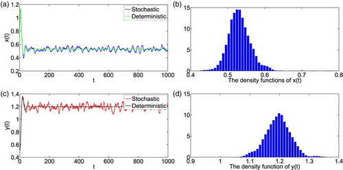
Figure 1. (a) and (c): The asymptotic behaviour of the solutions to stochastic model (2) around the positive equilibrium of model (1) with initial value $\left(x\right(0),y(0\left)\right)=(0.6,0.5)$; (b) and (d): The density function diagrams of $x\left(t\right)$ and $y\left(t\right)$, respectively. The parameters are taken as (23(23) $\alpha =0.6,b=0.3,\text{β}=0.3,c=0.8,a=0.3,\gamma =0.1,$(23) ) and m = 0.1, K = 0.3, ${\sigma }_1={\sigma }_2=0.01$.

To obtain deep insights of the influences of white noise on population dynamics, we keep the model parameter values the same as in (23(23) $\alpha =0.6,b=0.3,\text{β}=0.3,c=0.8,a=0.3,\gamma =0.1,$(23) ) but let ${\sigma }_1=1.1$, which implies that condition $\alpha <{\sigma }_1^2/2$ holds. Then we get that both prey and predator populations are extinction by Theorem 4.1, shown as in Figure 2. 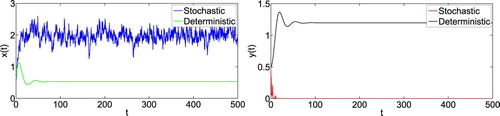Now we take ${\sigma }_1=0.1,{\sigma }_2=0.9$ and the other parameters remain unchanged, we can easily check that the condition $\alpha >{\sigma }_1^2/2,c\text{β}(1-m)\left(\right(\alpha -\left({\sigma }_1^2/2\right)/b)-\gamma -\frac{{\sigma }_2^2}{2}<0$ are satisfied. By Theorem 4.1, we know that the prey population is persistent and the predator population will be extinct (see Figure 3). These show that the random disturbance will change the dynamics when the environment noise is large enough.

Figure 2. Numerical simulation for model (1(1) $\begin{array}{rl}\frac{\mathrm{d}x}{\mathrm{d}t}& =\frac{\alpha x}{1+Ky}-b{x}^2-\frac{\text{β}(1-m)xy}{1+a(1-m)x},\\ \frac{\mathrm{d}y}{\mathrm{d}t}& =-\gamma y+\frac{c\text{β}(1-m)xy}{1+a(1-m)x},\end{array}$(1) ) and model (2(2) $\begin{array}{rl}\mathrm{d}x& =\left[\frac{\alpha x}{1+Ky}-b{x}^2-\frac{\text{β}(1-m)xy}{1+a(1-m)x}\right]\mathrm{d}t+{\sigma }_{1}x\mathrm{d}{B}_1\left(t\right),\\ \mathrm{d}y& =\left[-\gamma y+\frac{c\text{β}(1-m)xy}{1+a(1-m)x}\right]\mathrm{d}t+{\sigma }_{2}y\mathrm{d}{B}_2\left(t\right),\end{array}$(2) ) with initial value $\left(x\right(0),y(0\left)\right)=(0.6,0.5)$. The parameters are taken as (23(23) $\alpha =0.6,b=0.3,\text{β}=0.3,c=0.8,a=0.3,\gamma =0.1,$(23) ) and m = 0.1, K = 0.3, ${\sigma }_1=1.1$, ${\sigma }_2=0.01$.

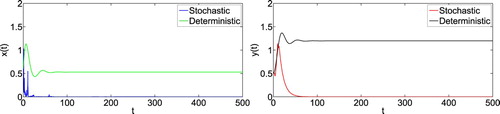
Figure 3. Numerical simulation for model (1(1) $\begin{array}{rl}\frac{\mathrm{d}x}{\mathrm{d}t}& =\frac{\alpha x}{1+Ky}-b{x}^2-\frac{\text{β}(1-m)xy}{1+a(1-m)x},\\ \frac{\mathrm{d}y}{\mathrm{d}t}& =-\gamma y+\frac{c\text{β}(1-m)xy}{1+a(1-m)x},\end{array}$(1) ) and model (2(2) $\begin{array}{rl}\mathrm{d}x& =\left[\frac{\alpha x}{1+Ky}-b{x}^2-\frac{\text{β}(1-m)xy}{1+a(1-m)x}\right]\mathrm{d}t+{\sigma }_{1}x\mathrm{d}{B}_1\left(t\right),\\ \mathrm{d}y& =\left[-\gamma y+\frac{c\text{β}(1-m)xy}{1+a(1-m)x}\right]\mathrm{d}t+{\sigma }_{2}y\mathrm{d}{B}_2\left(t\right),\end{array}$(2) ) with initial value $\left(x\right(0),y(0\left)\right)=(0.6,0.5)$. The parameters are taken as (23(23) $\alpha =0.6,b=0.3,\text{β}=0.3,c=0.8,a=0.3,\gamma =0.1,$(23) ) and m = 0.1, K = 0.3, ${\sigma }_1=0.1$, ${\sigma }_2=0.9$.

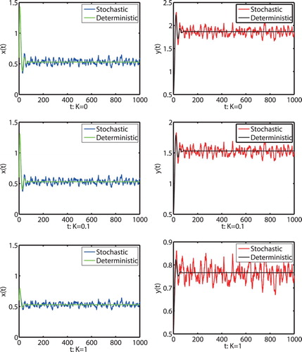
Next, in order to illustrate the influence of fear effect to model (2(2) $\begin{array}{rl}\mathrm{d}x& =\left[\frac{\alpha x}{1+Ky}-b{x}^2-\frac{\text{β}(1-m)xy}{1+a(1-m)x}\right]\mathrm{d}t+{\sigma }_{1}x\mathrm{d}{B}_1\left(t\right),\\ \mathrm{d}y& =\left[-\gamma y+\frac{c\text{β}(1-m)xy}{1+a(1-m)x}\right]\mathrm{d}t+{\sigma }_{2}y\mathrm{d}{B}_2\left(t\right),\end{array}$(2) ) through numerical simulation, we choose different values of K, say K = 0, K = 0.1 and K = 1, ${\sigma }_1={\sigma }_2=0.01$. For the remaining parameter values, we keep them the same as in (23(23) $\alpha =0.6,b=0.3,\text{β}=0.3,c=0.8,a=0.3,\gamma =0.1,$(23) ). We can compute that these parameters satisfy Assumptions $\left(H_1\right)$ and $\left(H_2\right)$ and therefore model (2(2) $\begin{array}{rl}\mathrm{d}x& =\left[\frac{\alpha x}{1+Ky}-b{x}^2-\frac{\text{β}(1-m)xy}{1+a(1-m)x}\right]\mathrm{d}t+{\sigma }_{1}x\mathrm{d}{B}_1\left(t\right),\\ \mathrm{d}y& =\left[-\gamma y+\frac{c\text{β}(1-m)xy}{1+a(1-m)x}\right]\mathrm{d}t+{\sigma }_{2}y\mathrm{d}{B}_2\left(t\right),\end{array}$(2) ) has a stationary distribution, which means that both prey and predator populations are persistent. Moreover, from Figure 4 we find that the increase of fear effect will reduce the density of predator but with no obvious effect on the density of prey.

Figure 4. Numerical simulation for model (1(1) $\begin{array}{rl}\frac{\mathrm{d}x}{\mathrm{d}t}& =\frac{\alpha x}{1+Ky}-b{x}^2-\frac{\text{β}(1-m)xy}{1+a(1-m)x},\\ \frac{\mathrm{d}y}{\mathrm{d}t}& =-\gamma y+\frac{c\text{β}(1-m)xy}{1+a(1-m)x},\end{array}$(1) ) and model (2(2) $\begin{array}{rl}\mathrm{d}x& =\left[\frac{\alpha x}{1+Ky}-b{x}^2-\frac{\text{β}(1-m)xy}{1+a(1-m)x}\right]\mathrm{d}t+{\sigma }_{1}x\mathrm{d}{B}_1\left(t\right),\\ \mathrm{d}y& =\left[-\gamma y+\frac{c\text{β}(1-m)xy}{1+a(1-m)x}\right]\mathrm{d}t+{\sigma }_{2}y\mathrm{d}{B}_2\left(t\right),\end{array}$(2) ) with initial value $\left(x\right(0),y(0\left)\right)=(0.6,0.5)$ and different K, respectively. The parameters are taken as (23(23) $\alpha =0.6,b=0.3,\text{β}=0.3,c=0.8,a=0.3,\gamma =0.1,$(23) ) and m = 0.1, ${\sigma }_1={\sigma }_2=0.01$.

Finally, we numerically illustrate the impact of a prey refuge to model (2(2) $\begin{array}{rl}\mathrm{d}x& =\left[\frac{\alpha x}{1+Ky}-b{x}^2-\frac{\text{β}(1-m)xy}{1+a(1-m)x}\right]\mathrm{d}t+{\sigma }_{1}x\mathrm{d}{B}_1\left(t\right),\\ \mathrm{d}y& =\left[-\gamma y+\frac{c\text{β}(1-m)xy}{1+a(1-m)x}\right]\mathrm{d}t+{\sigma }_{2}y\mathrm{d}{B}_2\left(t\right),\end{array}$(2) ) and choose different values of m, say m = 0, m = 0.2, m = 0.5 and m = 0.7, ${\sigma }_1={\sigma }_2=0.01$. For the remaining parameter values, we keep them the same as in (23(23) $\alpha =0.6,b=0.3,\text{β}=0.3,c=0.8,a=0.3,\gamma =0.1,$(23) ). We can easily compute that these parameters satisfy assumptions $\left(H_1\right)$ and $\left(H_2\right)$. 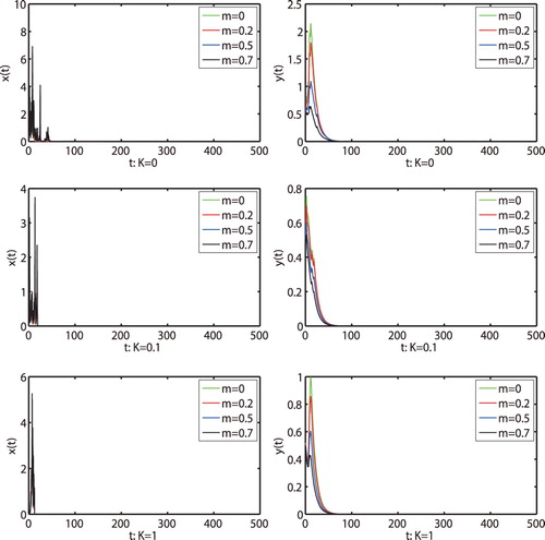So we obtain that there is a unique ergodic stationary distribution for model (2(2) $\begin{array}{rl}\mathrm{d}x& =\left[\frac{\alpha x}{1+Ky}-b{x}^2-\frac{\text{β}(1-m)xy}{1+a(1-m)x}\right]\mathrm{d}t+{\sigma }_{1}x\mathrm{d}{B}_1\left(t\right),\\ \mathrm{d}y& =\left[-\gamma y+\frac{c\text{β}(1-m)xy}{1+a(1-m)x}\right]\mathrm{d}t+{\sigma }_{2}y\mathrm{d}{B}_2\left(t\right),\end{array}$(2) ), which means that both prey and predator populations are persistent. From Figure 5, we can see that with the increase of the amount of refuges m, the density of the prey increases while the predator density decreases. This means that the increase of the amount of refuges m is favourable to prey population but it is adverse to the persistence of predator population. Moreover, we can also see that large K may lead to the predator density decreasing fast. When we choose ${\sigma }_1=1.1,{\sigma }_2=0.01$ and the other parameters are the same as in Figure 5, we simply calculate that condition $\alpha <{\sigma }_1^2/2$ holds. Then we obtain that both prey and predator populations are extinction by Theorem 4.1, shown in Figure 6. The results again show that the large noise is very destructive to the persistence of the population.

Figure 5. The solutions of model (2(2) $\begin{array}{rl}\mathrm{d}x& =\left[\frac{\alpha x}{1+Ky}-b{x}^2-\frac{\text{β}(1-m)xy}{1+a(1-m)x}\right]\mathrm{d}t+{\sigma }_{1}x\mathrm{d}{B}_1\left(t\right),\\ \mathrm{d}y& =\left[-\gamma y+\frac{c\text{β}(1-m)xy}{1+a(1-m)x}\right]\mathrm{d}t+{\sigma }_{2}y\mathrm{d}{B}_2\left(t\right),\end{array}$(2) ) with the initial value $\left(x\right(0),y(0\left)\right)=(0.6,0.5)$ and different K,m, respectively. The parameters are taken as (23(23) $\alpha =0.6,b=0.3,\text{β}=0.3,c=0.8,a=0.3,\gamma =0.1,$(23) ) and ${\sigma }_1={\sigma }_2=0.01$.

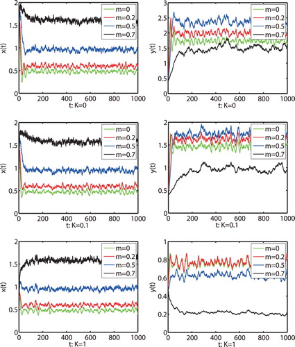
Figure 6. The solutions of model (2(2) $\begin{array}{rl}\mathrm{d}x& =\left[\frac{\alpha x}{1+Ky}-b{x}^2-\frac{\text{β}(1-m)xy}{1+a(1-m)x}\right]\mathrm{d}t+{\sigma }_{1}x\mathrm{d}{B}_1\left(t\right),\\ \mathrm{d}y& =\left[-\gamma y+\frac{c\text{β}(1-m)xy}{1+a(1-m)x}\right]\mathrm{d}t+{\sigma }_{2}y\mathrm{d}{B}_2\left(t\right),\end{array}$(2) ) with the initial value $\left(x\right(0),y(0\left)\right)=(0.6,0.5)$ and different K,m, respectively. The parameters are taken as (23(23) $\alpha =0.6,b=0.3,\text{β}=0.3,c=0.8,a=0.3,\gamma =0.1,$(23) ) and ${\sigma }_1=1.1,{\sigma }_2=0.01$.

6. Conclusion

This paper focuses on a stochastic Holling type-II prey–predator model with a prey refuge and fear effect. Mathematically, the sufficient criteria for the existence of a unique ergodic stationary distribution and the extinction of the model have been obtained. Ecologically, we get the following conclusions:

1. Random disturbance may change the dynamic behaviour of the population, especially when the noise is large, it may lead to the extinction of the prey and predator populations.

2. By simulations, we find that the increase of fear effect K will reduce the density of predator, but the effect on the density of prey is not obvious. In addition, one can see that the increase of the amount of refuges m is favourable to prey population but it is adverse to the persistence of predator population.

There are some interesting themes worthy of further research. On the one hand, we can incorporate some other environmental noises into model (2(2) $\begin{array}{rl}\mathrm{d}x& =\left[\frac{\alpha x}{1+Ky}-b{x}^2-\frac{\text{β}(1-m)xy}{1+a(1-m)x}\right]\mathrm{d}t+{\sigma }_{1}x\mathrm{d}{B}_1\left(t\right),\\ \mathrm{d}y& =\left[-\gamma y+\frac{c\text{β}(1-m)xy}{1+a(1-m)x}\right]\mathrm{d}t+{\sigma }_{2}y\mathrm{d}{B}_2\left(t\right),\end{array}$(2) ), such as coloured noise, Poisson noise and so on. On the other hand, to make the model (2(2) $\begin{array}{rl}\mathrm{d}x& =\left[\frac{\alpha x}{1+Ky}-b{x}^2-\frac{\text{β}(1-m)xy}{1+a(1-m)x}\right]\mathrm{d}t+{\sigma }_{1}x\mathrm{d}{B}_1\left(t\right),\\ \mathrm{d}y& =\left[-\gamma y+\frac{c\text{β}(1-m)xy}{1+a(1-m)x}\right]\mathrm{d}t+{\sigma }_{2}y\mathrm{d}{B}_2\left(t\right),\end{array}$(2) ) more realistic, we can further consider the factors such as the influence of impulsive perturbations and delay. We leave these for future investigations.

Disclosure statement

No potential conflict of interest was reported by the author(s).

Additional information

Funding

Research is supported by the National Natural Science Foundation of China (Grant Nos. 11671260 and 12071293).

Appendix 1: Construction of the stochastic model (2)

By the methods used in Ref. [6] about stochastic effects, we first consider a discrete time Markov chain. For $x\left(t\right)$ and $y\left(t\right)$ in model (2(2) $\begin{array}{rl}\mathrm{d}x& =\left[\frac{\alpha x}{1+Ky}-b{x}^2-\frac{\text{β}(1-m)xy}{1+a(1-m)x}\right]\mathrm{d}t+{\sigma }_{1}x\mathrm{d}{B}_1\left(t\right),\\ \mathrm{d}y& =\left[-\gamma y+\frac{c\text{β}(1-m)xy}{1+a(1-m)x}\right]\mathrm{d}t+{\sigma }_{2}y\mathrm{d}{B}_2\left(t\right),\end{array}$(2) ), given $\mathrm{\Delta }t>0$, we present a process $X^{\left(\mathrm{\Delta }t\right)}\left(t\right)=\left(x^{\left(\mathrm{\Delta }t\right)}\right(t),y^{\left(\mathrm{\Delta }t\right)}(t){)}^T,t=0,\mathrm{\Delta }t,2\mathrm{\Delta }t,\dots$with initial value $X^{\left(\mathrm{\Delta }t\right)}\left(0\right)=\left(x^{\left(\mathrm{\Delta }t\right)}\right(0),y^{\left(\mathrm{\Delta }t\right)}(0){)}^T\in {\mathbb{R}}_{+}^2$. Let normal distribution random variable sequence $\left\{R_i^{\left(\mathrm{\Delta }t\right)}\right(l){\}}_{l=0}^{\mathrm{\infty }}$ satisfies (A1) $\mathbb{E}\left[R_i^{\left(\mathrm{\Delta }t\right)}\right(l\left)\right]=0,\mathbb{E}\left[R_i^{\left(\mathrm{\Delta }t\right)}\right(l){]}^2={\sigma }_i^2\mathrm{\Delta }t,\mathbb{E}[R_i^{\left(\mathrm{\Delta }t\right)}\left(l\right){]}^4=o\left(\mathrm{\Delta }t\right),$(A1) where $i=1,2,$ $l=0,1,2,\dots$ and ${\sigma }_i^2$ express the intensities of stochastic effects. On each period $[l\mathrm{\Delta }t,(l+1\left)\mathrm{\Delta }t\right)$, we assume that $X^{\left(\mathrm{\Delta }t\right)}\left(t\right)$ grows according to model (2(2) $\begin{array}{rl}\mathrm{d}x& =\left[\frac{\alpha x}{1+Ky}-b{x}^2-\frac{\text{β}(1-m)xy}{1+a(1-m)x}\right]\mathrm{d}t+{\sigma }_{1}x\mathrm{d}{B}_1\left(t\right),\\ \mathrm{d}y& =\left[-\gamma y+\frac{c\text{β}(1-m)xy}{1+a(1-m)x}\right]\mathrm{d}t+{\sigma }_{2}y\mathrm{d}{B}_2\left(t\right),\end{array}$(2) ) and is also affected by the random $\left(x^{\left(\mathrm{\Delta }t\right)}{R}_1^{\left(\mathrm{\Delta }t\right)}\right(l),y^{\left(\mathrm{\Delta }t\right)}{R}_2^{\left(\mathrm{\Delta }t\right)}(l){)}^T$. Specifically, for $l=0,1,\dots$, we get $\begin{array}{rl}{x}^{\left(\mathrm{\Delta }t\right)}\left(\right(l+1\left)\mathrm{\Delta }t\right)& =x^{\left(\mathrm{\Delta }t\right)}\left(l\mathrm{\Delta }t\right)+x^{\left(\mathrm{\Delta }t\right)}\left(l\mathrm{\Delta }t\right)R_1^{\left(\mathrm{\Delta }t\right)}\left(l\right)\\ & +\left[x^{\left(\mathrm{\Delta }t\right)}\left(l\mathrm{\Delta }t\right)\left(\frac{\alpha }{1+K{y}^{\left(\mathrm{\Delta }t\right)}\left(l\mathrm{\Delta }t\right)}-b{x}^{\left(\mathrm{\Delta }t\right)}\left(l\mathrm{\Delta }t\right)\right.\right.\\ & -\left.\left.\frac{\text{β}(1-m)y^{\left(\mathrm{\Delta }t\right)}\left(l\mathrm{\Delta }t\right)}{1+a(1-m)x^{\left(\mathrm{\Delta }t\right)}\left(l\mathrm{\Delta }t\right)}\right)\right]\mathrm{\Delta }t,\\ y^{\left(\mathrm{\Delta }t\right)}\left(\right(l+1\left)\mathrm{\Delta }t\right)& =y^{\left(\mathrm{\Delta }t\right)}\left(l\mathrm{\Delta }t\right)+y^{\left(\mathrm{\Delta }t\right)}\left(l\mathrm{\Delta }t\right)R_2^{\left(\mathrm{\Delta }t\right)}\left(l\right)\\ & +\left[-\gamma y^{\left(\mathrm{\Delta }t\right)}\left(l\mathrm{\Delta }t\right)+\frac{c\text{β}(1-m)x^{\left(\mathrm{\Delta }t\right)}\left(l\mathrm{\Delta }t\right)y^{\left(\mathrm{\Delta }t\right)}\left(l\mathrm{\Delta }t\right)}{1+a(1-m)x^{\left(\mathrm{\Delta }t\right)}\left(l\mathrm{\Delta }t\right)}\right]\mathrm{\Delta }t.\end{array}$Next we demonstrate that $X^{\left(\mathrm{\Delta }t\right)}\left(t\right)$ converges to a diffusion process as $\mathrm{\Delta }t\to 0$. And we need to determine the drift coefficient and diffusion coefficient of the diffusion process. Let ${\mathcal{P}}^{\left(\mathrm{\Delta }t\right)}(\overline{x},dz)$ denote the transition probabilities of the homogeneous Markov chain $\left\{X^{\left(\mathrm{\Delta }t\right)}\right(l\mathrm{\Delta }t\left)\right\}$, that is ${\mathcal{P}}^{\left(\mathrm{\Delta }t\right)}(\overline{x},B)=\mathrm{P}\mathrm{r}\mathrm{o}\mathrm{b}\left\{X^{\left(\mathrm{\Delta }t\right)}\right((l+1)\mathrm{\Delta }t)\in B|X^{\left(\mathrm{\Delta }t\right)}=\overline{x}\}$for all $\overline{x}=(x,y)\in {\mathbb{R}}_{+}^2$ and all Borel sets $B\subset {\mathbb{R}}_{+}^2$. From (A1(A1) $\mathbb{E}\left[R_i^{\left(\mathrm{\Delta }t\right)}\right(l\left)\right]=0,\mathbb{E}\left[R_i^{\left(\mathrm{\Delta }t\right)}\right(l){]}^2={\sigma }_i^2\mathrm{\Delta }t,\mathbb{E}[R_i^{\left(\mathrm{\Delta }t\right)}\left(l\right){]}^4=o\left(\mathrm{\Delta }t\right),$(A1) ) $\begin{array}{rl}\frac{1}{\mathrm{\Delta }t}\int (z_1-x){\mathcal{P}}^{\left(\mathrm{\Delta }t\right)}(\overline{x},\mathrm{d}z)& =x\left(\frac{\alpha }{1+ky}-bx-\frac{\text{β}(1-m)y}{1+a(1-m)x}\right)+\frac{x}{\mathrm{\Delta }t}\mathbb{E}{R}_1^{\left(\mathrm{\Delta }t\right)}\left(0\right)\\ & =x\left(\frac{\alpha }{1+ky}-bx-\frac{\text{β}(1-m)y}{1+a(1-m)x}\right),\\ \frac{1}{\mathrm{\Delta }t}\int (z_2-y){\mathcal{P}}^{\left(\mathrm{\Delta }t\right)}(\overline{x},\mathrm{d}z)& =-\gamma y+\frac{c\text{β}(1-m)xy}{1+a(1-m)x}+\frac{y}{\mathrm{\Delta }t}\mathbb{E}{R}_2^{\left(\mathrm{\Delta }t\right)}\left(0\right)\\ & =-\gamma y+\frac{c\text{β}(1-m)xy}{1+a(1-m)x}.\end{array}$To determine the diffusion coefficients, we consider the following moments: $g_{ij}^{\left(\mathrm{\Delta }t\right)}\left(x\right)=\frac{1}{\mathrm{\Delta }t}\int (z_i-x_i)(z_j-x_j){\mathcal{P}}^{\left(\mathrm{\Delta }t\right)}(x,\mathrm{d}z),i,j=1,2.$By (A1(A1) $\mathbb{E}\left[R_i^{\left(\mathrm{\Delta }t\right)}\right(l\left)\right]=0,\mathbb{E}\left[R_i^{\left(\mathrm{\Delta }t\right)}\right(l){]}^2={\sigma }_i^2\mathrm{\Delta }t,\mathbb{E}[R_i^{\left(\mathrm{\Delta }t\right)}\left(l\right){]}^4=o\left(\mathrm{\Delta }t\right),$(A1) ) $\begin{array}{rl}\left|g_{11}^{\left(\mathrm{\Delta }t\right)}\left(x\right)-{\sigma }_1^2{x}^2\right|& =\left|\frac{1}{\mathrm{\Delta }t}\mathbb{E}\{\mathrm{\Delta }t\left[x\left(\frac{\alpha }{1+Ky}-bx-\frac{\text{β}(1-m)y}{1+a(1-m)x}\right)\right]+R_1^{\left(\mathrm{\Delta }t\right)}\left(0\right)x{\}}^2-{\sigma }_1^2{x}^2\right|\\ & =|\mathrm{\Delta }t{\left[x\left(\frac{\alpha }{1+Ky}-bx-\frac{\text{β}(1-m)y}{1+a(1-m)x}\right)\right]}^2\\ & +2x^2\left(\frac{\alpha }{1+Ky}-bx-\frac{\text{β}(1-m)y}{1+a(1-m)x}\right)\mathbb{E}{R}_1^{\left(\mathrm{\Delta }t\right)}\left(0\right)\\ & +\frac{1}{\mathrm{\Delta }t}{x}^2\mathbb{E}{\left[R_1^{\left(\mathrm{\Delta }t\right)}\left(0\right)\right]}^2-{\sigma }_1^2{x}^2|\\ & =\mathrm{\Delta }t{\left[x\left(\frac{\alpha }{1+Ky}-bx-\frac{\text{β}(1-m)y}{1+a(1-m)x}\right)\right]}^2,\\ \left|g_{22}^{\left(\mathrm{\Delta }t\right)}\left(x\right)-{\sigma }_2^2{y}^2\right|& =\left|\frac{1}{\mathrm{\Delta }t}\mathbb{E}\{\mathrm{\Delta }t\left[-\gamma y+\frac{c\text{β}(1-m)xy}{1+a(1-m)x}\right]+R_2^{\left(\mathrm{\Delta }t\right)}\left(0\right)y{\}}^2-{\sigma }_2^2{y}^2\right|\\ & =|\mathrm{\Delta }t{\left[-\gamma y+\frac{c\text{β}(1-m)xy}{1+a(1-m)x}\right]}^2+2y^2\left[-\gamma +\frac{c\text{β}(1-m)x}{1+a(1-m)x}\right]\mathbb{E}{R}_2^{\left(\mathrm{\Delta }t\right)}\left(0\right)\\ & +\frac{1}{\mathrm{\Delta }t}{y}^2\mathbb{E}{\left[R_2^{\left(\mathrm{\Delta }t\right)}\left(0\right)\right]}^2-{\sigma }_2^2{y}^2|\\ & =\mathrm{\Delta }t{\left[-\gamma y+\frac{c\text{β}(1-m)xy}{1+a(1-m)x}\right]}^2.\end{array}$Therefore, $\underset{\mathrm{\Delta }t\to 0^{+}}{lim}\underset{||x||\le L}{sup}\left|g_{11}^{\left(\mathrm{\Delta }t\right)}\left(x\right)-{\sigma }_1^2{x}^2\right|=0,\underset{\mathrm{\Delta }t\to 0^{+}}{lim}\underset{||x||\le L}{sup}\left|g_{22}^{\left(\mathrm{\Delta }t\right)}\left(x\right)-{\sigma }_2^2{y}^2\right|=0$for all $0<L<\mathrm{\infty }$. Similarly, $\underset{\mathrm{\Delta }t\to 0^{+}}{lim}\underset{||x||\le L}{sup}\left|g_{12}^{\left(\mathrm{\Delta }t\right)}\left(x\right)\right|=0.$In addition, from (A1(A1) $\mathbb{E}\left[R_i^{\left(\mathrm{\Delta }t\right)}\right(l\left)\right]=0,\mathbb{E}\left[R_i^{\left(\mathrm{\Delta }t\right)}\right(l){]}^2={\sigma }_i^2\mathrm{\Delta }t,\mathbb{E}[R_i^{\left(\mathrm{\Delta }t\right)}\left(l\right){]}^4=o\left(\mathrm{\Delta }t\right),$(A1) ), we obtain that for all $0<L<\mathrm{\infty }$ $\underset{\mathrm{\Delta }t\to 0^{+}}{lim}\underset{||x||\le L}{sup}\frac{1}{\mathrm{\Delta }t}\int ||z-x|{|}^3{\mathcal{P}}^{\left(\mathrm{\Delta }t\right)}(x,\mathrm{d}z)=0.$Finally, extend the definition of $X^{\left(\mathrm{\Delta }t\right)}\left(t\right)$ to all $t\ge 0$ by setting $X^{\left(\mathrm{\Delta }t\right)}\left(t\right)=X^{\left(\mathrm{\Delta }t\right)}\left(l\mathrm{\Delta }t\right)$ for all $t\in [l\mathrm{\Delta }t,(l+1\left)\mathrm{\Delta }t\right)$. On the basis of Theorem 7.1, Lemma 8.2 in Ref. [6], we can verify that as $t\to 0$, $X^{\left(\mathrm{\Delta }t\right)}\left(t\right)$ converges weakly to the solution of the stochastic system as follows: $\begin{array}{rl}\mathrm{d}x& =\left[\frac{\alpha x}{1+Ky}-b{x}^2-\frac{\text{β}(1-m)xy}{1+a(1-m)x}\right]\mathrm{d}t+{\sigma }_{1}x\mathrm{d}{B}_1\left(t\right),\\ \mathrm{d}y& =\left[-\gamma y+\frac{c\text{β}(1-m)xy}{1+a(1-m)x}\right]\mathrm{d}t+{\sigma }_{2}y\mathrm{d}{B}_2\left(t\right),\end{array}$where $B_1\left(t\right)$ and $B_2\left(t\right)$ are two independent Brownian motions with the intensities represented by two positive constants ${\sigma }_1$ and ${\sigma }_2$.

References

- J.R. Beddington, Mutual interference between parasites or predators and its effect on searching efficiency, J. Anim. Ecol. 44 (1975), pp. 331–340.
- F. Brauer and C. Castillo-Chvez, Mathematical Models in Population Biology and Epidemiology, Springer, Berlin, 2001.
- S. Creel and D. Christianson, Relationships between direct predation and risk effects, Trends Ecol. Evol. 23 (2008), pp. 194–201.
- W. Cresswell, Predation in bird populations, J. Ornithol. 152 (2011), pp. 251–263.
- D.L. DeAngelis, R.A. Goldstein, and R.V. O'Neill, A model for tropic interaction, Ecology, 56 (1975), pp. 881–892.
- R. Durrett, Stochastic Calculus: A Practical Introduction, Probability Stochastics, 1st ed., CRC Press, Boca Raton, FL, 1996.
- R.Z. Has'minskii, Stochastic Stability of Differential Equations, Sijthoff Noordhoff, Alphen aan den Rijn, The Netherlands, 1980.
- D. Higham, An algorithmic introduction to numerical simulation of stochastic differential equations, SIAM Rev. 43 (2001), pp. 525–546.
- C.S. Holling, The functional response of predators to prey density and its role in mimicry and population regulation, Mem. Entomol. Soc. Can. 97 (1965), pp. 5–60.
- Y. Huang, F. Chen, and L. Zhong, Stability analysis of a prey–predator model with Holling type III response function incorporating a prey refuge, Appl. Math. Comput. 182 (2006), pp. 672–683.
- C. Ji and D. Jiang, Qualitative analysis of a stochastic ratio-dependent predator–prey system, J. Comput. Appl. Math. 235 (2011), pp. 1326–1341.
- D. Jia, T. Zhang, and S. Yuan, Pattern dynamics of a diffusive toxin producing phytoplankton–zooplankton model with three-dimensional patch, Int. J. Bifurcat. Chaos 29 (2019), pp. 1930011.
- S.L. Lima, Nonlethal effects in the ecology of predator–prey interactions, Bioscience 48 (1998), pp. 25–34.
- M. Liu and M. Deng, Permanence and extinction of a stochastic hybrid model for tumor growth, Appl. Math. Lett. 94 (2019), pp. 66–72.
- Q. Liu, D. Jiang, T. Hayat, and A. Alsaedi, Dynamics of a stochastic predator-prey model with stage structure for predator and Holling type II functional response, J. Nonlinear Sci. 28 (2018), pp. 1151–1187.
- C. Liu, L. Wang, Q. Zhang, and Y. Yan, Dynamical analysis in a bioeconomic phytoplankton zooplankton system with double time delays and environmental stochasticity, Physica A 15 (2017), pp. 682–698.
- M. Liu and Y. Zhu, Stability of a budworm growth model with random perturbations, Appl. Math. Lett. 79 (2018), pp. 13–19.
- Z. Ma, F. Chen, C. Wu, and W. Chen, Dynamic behaviors of a Lotka-Volterra predator–prey model incorporating a prey refuge and predator mutual interference, Appl. Math. Comput. 219 (2013), pp. 7945–7953.
- Z. Ma, S. Wang, W. Li, and Z. Li, The effect of prey refuge in a patchy predator–prey system, Math. Biosci. 243 (2013), pp. 126–130.
- X. Mao, Stochastic Differential Equations and Applications, Woodhead Publishing, Cambridge, 2007.
- X. Mao, G. Marion, and E. Renshaw, Environmental Brownian noise suppresses explosions in population dynamics, Stochast. Proc. Appl. 97 (2002), pp. 95–110.
- X. Meng, F. Li, and S. Gao, Global analysis and numerical simulations of a novel stochastic eco-epidemiological model with time delay, Appl. Math. Comput. 339 (2018), pp. 701–726.
- D. Mukherjee, The effect of prey refuges on a three species food chain model, Differ. Equ. Dyn. Syst.22 (2014), pp. 413–426.
- J. Ripa, P. Lundberg, and V. Kaitala, A general theory of environmental noise in ecological food webs, Am. Nat. 151 (1998), pp. 256–263.
- S. Sarwardi, P.K. Mandal, and S. Ray, Analysis of a competitive prey–predator system with a prey refuge, Biosystems 110 (2012), pp. 133–148.
- S. Sasmal, Population dynamics with multiple Allee effects induced by fear factors induced by fear factors – a mathematical study on prey–predator, Appl. Math. Model. 64 (2018), pp. 1–14.
- A. Sih, Prey refuges and predator–prey stability, Theor. Popul. Biol. 31 (1987), pp. 1–12.
- X. Wang, L. Zanette, and X. Zou, Modelling the fear effect in predator–prey interactions, J. Math. Biol. 73 (2016), pp. 1–38.
- C. Xu and S. Yuan, Competition in the chemostat: a stochastic multi-species model and its asymptotic behavior, Math. Biosci. 280 (2016), pp. 1–9.
- C. Xu, S. Yuan, and T. Zhang, Global dynamics of a predator–prey model with defence mechanism for prey, Appl. Math. Lett. 62 (2016), pp. 42–48.
- C. Xu, S. Yuan, and T. Zhang, Average break-even concentration in a simple chemostat model with telegraph noise, Nonlinear Anal. Hybrid. Syst. 29 (2018), pp. 373–382.
- S. Yan, D. Jia, T. Zhang, and S. Yuan, Pattern dynamic in a diffusive predator–prey model with hunting cooperations, Chaos Solitons Fract. 130 (2020), pp. 109428.
- F. Yi, J. Wei, and J. Shi, Bifurcation and spatiotemporal patterns in a homogeneous diffusive predator–prey system, J. Differ. Equ. 246 (2009), pp. 1944–1977.
- X. Yu and S. Yuan, Asymptotic properties of a stochastic chemostat model with two distributed delays and nonlinear perturbation, Discrete Contin. Dyn. B 25 (2020), pp. 2373–2390.
- X. Yu, S. Yuan, and T. Zhang, Asymptotic properties of stochastic nutrient-plankton food chain models with nutrient recycling, Nonlinear Anal. Hybrid. Syst. 34 (2019), pp. 209–225.
- S. Yuan, D. Wu, G. Lan, and H. Wang, Noise-induced transitions in a nonsmooth predator–prey model with stoichiometric constraints, Bull. Math. Biol. 82 (2020), pp. 167.
- H. Zhang, Y. Cai, S. Fu, and W. Wang, Impact of the fear effect in a prey–predator model incorporating a prey refuge, Appl. Math. Comput. 356 (2019), pp. 328–337.
- S. Zhang and X. Meng, Dynamics analysis and numerical simulations of a stochastic non-autonomous predator–prey system with impulsive effects, Nonlinear Anal. Hybrid. Syst. 26 (2017), pp. 19–37.
- Y. Zhao, S. Yuan, and J. Ma, Survival and stationary distribution analysis of a stochastic competitive model of three species in a polluted environment, Bull. Math. Biol. 77 (2015), pp. 1285–1326.
- S. Zhao, S. Yuan, and H. Wang, Threshold behavior in a stochastic algal growth model with stoichiometric constraints and seasonal variation, J. Differ. Equ. 268 (2020), pp. 5113–5139.
- W. Zuo and D. Jiang, Stationary distribution and periodic solution for stochastic predator–prey systems with nonlinear predator harvesting, Commun. Nonlinear Sci. 36 (2016), pp. 65–80.