A stochastic predator–prey model with Holling II increasing function in the predator

Abstract

This paper is concerned with a stochastic predator–prey model with Holling II increasing function in the predator. By applying the Lyapunov analysis method, we demonstrate the existence and uniqueness of the global positive solution. Then we show there is a stationary distribution which implies the stochastic persistence of the predator and prey in the model. Moreover, we obtain respectively sufficient conditions for weak persistence in the mean and extinction of the prey and extinction of the predator. Finally, some numerical simulations are given to illustrate our main results and the discussion and conclusion are presented.

Keywords:

• Stochastic predator–prey model
• Holling II increasing function in the predator
• the global positive solution
• persistence and extinction

2010 AMS Subject Classifications:

• 60H10
• 92D25

1. Introduction

The dynamical relationship between predators and preys is one of the most important and interesting topics in biomathematics [20]. Some models have been presented, which study a two-dimension predator–prey model [16, 29,40], multi-predator model [7,35] or multi-prey model [13,33, 39]. The dynamic property of a predator–prey model with the disease spreading is also one of the dominant themes in biomathematics. To study the effects of disease on the population, these models with sick prey or sick predators have been studied [10,11, 18, 34,45,46]. In addition, some models with the functional responses have also been proposed [8, 19, 29, 30]. Many conclusions have been drawn and are expected to become more substantial in the future.

The relationship between pests and their natural enemies is a typical predator–prey relationship. In agriculture, how to control pests is a key point. Among the pest control methods, biological control is a common approach. There has been a lot of research and some good results [14,37,38, 44].

Tang [37] proposed a pest management predator–prey model with the prey-dependent consumption and established the following ODE model with Holling II increasing function in the predator: (1) $\begin{array}{rl}& \frac{\mathrm{d}x}{\mathrm{d}t}=x(r-by),\\ & \frac{\mathrm{d}y}{\mathrm{d}t}=\frac{\lambda bxy}{1+bhx}-d_{1}y,\end{array}$(1) where $x\left(t\right)$ and $y\left(t\right)$ represented the densities of the prey and the predator at time t, respectively; r was the growth rate of $x\left(t\right)$; the prey's contribution to the predator's growth rate was $\frac{\lambda bxy}{1+bhx}$, where b and h respectively denoted the searching rate and handling time, parameter λ was the rate at which ingested prey in excess of what was needed for maintenance was translated into predator population increase; $d_1$ denoted the mortality of $y\left(t\right)$; r, b, h, λ and $d_1$ were positive constants.

It was assumed that predators may consume a progressively smaller proportion of prey when the prey density increased [37]. And Tang proposed that this model had the same dynamical behaviour as the classical model.

To understand the effect of individual competition for a limited amount of food and living space, the environment capacity is taken into account in [17, 21,25,41]. Sun et al. [36] studied the following model with Holling II increasing function in the predator: (2) $\begin{array}{rl}& \frac{\mathrm{d}x}{\mathrm{d}t}=x\left(r-\frac{rx}{K}-by\right),\\ & \frac{\mathrm{d}y}{\mathrm{d}t}=y\left(\frac{\lambda bx}{1+bhx}-d_1\right).\end{array}$(2) where K was the environment capacity and other parameters were the same as the model (1(1) $\begin{array}{rl}& \frac{\mathrm{d}x}{\mathrm{d}t}=x(r-by),\\ & \frac{\mathrm{d}y}{\mathrm{d}t}=\frac{\lambda bxy}{1+bhx}-d_{1}y,\end{array}$(1) ). If $0\le h\le \frac{\lambda }{d_1}$, system (2(2) $\begin{array}{rl}& \frac{\mathrm{d}x}{\mathrm{d}t}=x\left(r-\frac{rx}{K}-by\right),\\ & \frac{\mathrm{d}y}{\mathrm{d}t}=y\left(\frac{\lambda bx}{1+bhx}-d_1\right).\end{array}$(2) ) has three equilibrium points $O(0,0),A(K,0),E^{\ast }(x^{\ast },y^{\ast })=\left(\frac{d_1}{b(\lambda -h{d}_1)},\frac{r\left[Kb\right(\lambda -h{d}_1)-d_1]}{K{b}^2(\lambda -h{d}_1)}\right).$Furthermore, $O(0,0)$, $A(K,0)$ are saddle points and $E^{\ast }(x^{\ast },y^{\ast })$ is a globally asymptotically stable focus [36].

In fact, population dynamics is inevitably affected by environmental white noise which is an important component in an ecosystem [12]. But in the deterministic model, all parameters are not disturbed by the environment. Hence the deterministic model has some limitations in mathematical modelling of ecological systems and is quite difficult to fitting data perfectly and to predict the future dynamics of the system accurately [1]. May [32] pointed out the fact that the birth rate, death rate, carrying capacity and other parameters in the system are affected by random fluctuations. To understand the impacts of randomness and fluctuations, it is convenient and effective to model population dynamics through a stochastic differential equation [17,22–24, 26–28,42].

In order to study the influence of environmental disturbance on the population, we introduce the method of [47]. For model (2(2) $\begin{array}{rl}& \frac{\mathrm{d}x}{\mathrm{d}t}=x\left(r-\frac{rx}{K}-by\right),\\ & \frac{\mathrm{d}y}{\mathrm{d}t}=y\left(\frac{\lambda bx}{1+bhx}-d_1\right).\end{array}$(2) ), given $\mathrm{\Delta }t>0$ and time instant $t=j\mathrm{\Delta }t$, introduce $X^j=(x^j,y^j)=\left(x\right(j\mathrm{\Delta }t),y(j\mathrm{\Delta }t){)}^{\mathrm{T}}$, $j=0,1,\dots$ with initial value $X^0=\left(x\right(0),y(0){)}^{\mathrm{T}}\in {\mathbb{R}}_{+}^2$, where ${\mathbb{R}}_{+}^2=\{X=(x_1,x_2)\in {\mathbb{R}}^2;x_i>0,i=1,2\}$. Let normal distribution random variable sequence $\left\{R_i^j\right(m){\}}_{m=0}^{\mathrm{\infty }}$ satisfy $E\left[R_i^{\mathrm{\Delta }t}\right(m\left)\right]=0$, $E\left[R_i^{\mathrm{\Delta }t}\right(m){]}^2={\sigma }_i^2\mathrm{\Delta }t$, $E\left[R_i^{\mathrm{\Delta }t}\right(m){]}^4=o(\mathrm{\Delta }t)$, where i = 1, 2 and $m=0,1,2,\dots$, and ${\sigma }_i^2$ denote the intensities of stochastic disturbance. In each interval $[m\mathrm{\Delta }t,(m+1\left)\mathrm{\Delta }t\right)$, assume that $X^{\left(j\right)}$ increases according to model (2(2) $\begin{array}{rl}& \frac{\mathrm{d}x}{\mathrm{d}t}=x\left(r-\frac{rx}{K}-by\right),\\ & \frac{\mathrm{d}y}{\mathrm{d}t}=y\left(\frac{\lambda bx}{1+bhx}-d_1\right).\end{array}$(2) ) and is also affected by the random amount $\left(x^m{R}_1^{\mathrm{\Delta }t}\right(m),y^m{R}_1^{\mathrm{\Delta }t}(m){)}^{\mathrm{T}}$. Hence, for $m=0,1,\dots$ we get $\begin{array}{rl}{x}^{m+1}& =x^m+x^m{R}_1^{\mathrm{\Delta }t}\left(m\right)+x^m\left(r-\frac{r{x}^m}{K}-b{y}^m\right)\mathrm{\Delta }t,\\ y^{m+1}& =y^m+y^m{R}_2^{\mathrm{\Delta }t}\left(m\right)+y^m\left(\frac{\lambda b{x}^m}{1+bh{x}^m}-d_1\right)\mathrm{\Delta }t.\end{array}$According to Theorem 7.1 and Lemma 8.2 in [6], as  $\mathrm{\Delta }t\to 0$, $X^m$ converges weakly to the solution of the following equation: (3) $\begin{array}{rl}\mathrm{d}x& =x\left(r-\frac{rx}{K}-by\right)\mathrm{d}t+{\sigma }_{1}x\mathrm{d}{B}_1\left(t\right),\\ \mathrm{d}y& =y\left(\frac{\lambda bx}{1+bhx}-d_1\right)\mathrm{d}t+{\sigma }_{2}y\mathrm{d}{B}_2\left(t\right),\end{array}$(3) where $B_i\left(t\right),i=1,2$ denote the standard independent Brownian motion.

The rest of this article is organized as follows. In Section 2, we give some definitions and lemmas to complete the structure of the article. In Section 3, the analytic results of dynamics of the stochastic predator–prey model are given which include the existence and uniqueness of the global positive solution, existence of the stationary distribution and the persistence and extinction of the prey and the extinction of the model (3(3) $\begin{array}{rl}\mathrm{d}x& =x\left(r-\frac{rx}{K}-by\right)\mathrm{d}t+{\sigma }_{1}x\mathrm{d}{B}_1\left(t\right),\\ \mathrm{d}y& =y\left(\frac{\lambda bx}{1+bhx}-d_1\right)\mathrm{d}t+{\sigma }_{2}y\mathrm{d}{B}_2\left(t\right),\end{array}$(3) ). We give some numerical simulations to verify our theoretical results in Section 4. Finally, we provide a brief discussion and the summary of the main results in Section 5.

2. Preliminaries

Throughout this paper, unless otherwise specified, we let $(\mathrm{\Omega },\mathcal{F},\{{\mathcal{F}}_t{\}}_{t\ge 0},P)$ be a complete probability space with a filtration $\{{\mathcal{F}}_t{\}}_{t\ge 0}$ satisfying the usual conditions (i.e. it is right continuous and ${\mathcal{F}}_0$ contains all P-null sets).

As a matter of convenience, we define some concepts and introduce some base definitions and symbols. Let ${\mathbb{R}}_{+}^n=\left\{X\right(t)=(x_1\left(t\right),x_2\left(t\right),\dots ,x_n\left(t\right))\in {\mathbb{R}}^n;x_i(t)>0,\mathrm{\forall }1\le i\le n\}$ and $|X\left(t\right)|=\sqrt{{\mathrm{\Sigma }}_{i=1}^n{x}_i^2\left(t\right)}$. In addition, for a function $z\left(t\right)$ for $t\in (0,\mathrm{\infty })$, define $〈z\left(t\right){〉}^{\ast }=\underset{t\to \mathrm{\infty }}{lim sup}\frac{1}{t}{\int }_0^{t}z\left(s\right)\mathrm{d}s,〈z\left(t\right){〉}_{\ast }=\underset{t\to \mathrm{\infty }}{lim inf}\frac{1}{t}{\int }_0^{t}z\left(s\right)\mathrm{d}s.$ First, some definitions and useful lemmas of permanence and extinction will be given.

Definition 2.1

[18, 25]

For the population $x\left(t\right)$:

1. If $\underset{t\to \mathrm{\infty }}{lim}x\left(t\right)=0$, then $x\left(t\right)$ is said to go to extinction almost surely.

2. If $〈x\left(t\right){〉}^{\ast }>0$, then $x\left(t\right)$ is weakly persistent in the mean almost surely.

Lemma 2.1

[31]

For $M=\{M_t{\}}_{t\ge 0}$ be a real-valued continuous local martingale vanishing at t = 0. Then

(i)	$\underset{t\to \mathrm{\infty }}{lim}\frac{M_t}{〈M,M{〉}_t}=0$ almost surely, if $\underset{t\to \mathrm{\infty }}{lim}〈M,M{〉}_t=\mathrm{\infty }$ almost surely.
(ii)	$\underset{t\to \mathrm{\infty }}{lim}\frac{M_t}{t}=0$ almost surely, if $\underset{t\to \mathrm{\infty }}{lim sup}\frac{〈M,M{〉}_t}{t}=\mathrm{\infty }$ almost surely.

Lemma 2.2

[4, 43]

Let $x\left(t\right)\in C[\mathrm{\Omega }\times [0,\mathrm{\infty }),(0,\mathrm{\infty }\left)\right]$. And there are $F\in C[\mathrm{\Omega }\times [0,\mathrm{\infty }),\mathbb{R}]$ and $\underset{t\to \mathrm{\infty }}{lim}\frac{F\left(t\right)}{t}=0$.

(i)

For all $t\ge 0,$ if there exist constant λ and positive constants T, ${\lambda }_0$ such that for all $t\ge T$ $\ln x\left(t\right)\le \lambda t-{\lambda }_0{\int }_0^{t}x\left(s\right)\mathrm{d}s+F\left(t\right)\mathit{\text{almost}}\mathit{\text{surely}},$then $\begin{array}{rl}& 〈x\left(t\right){〉}^{\ast }\le \frac{\lambda }{{\lambda }_0}\mathit{\text{almost}}\mathit{\text{surely}},\mathit{\text{if}}\lambda \ge 0,\\ & \underset{t\to \mathrm{\infty }}{lim}x\left(t\right)=0\mathit{\text{almost}}\mathit{\text{surely}},\mathit{\text{if}}\lambda <0.\end{array}$

(ii)

For all $t\ge 0,$ if there exist positive constants T, λ and ${\lambda }_0$ such that for all $t\ge T$ $\ln x\left(t\right)\ge \lambda t-{\lambda }_0{\int }_0^{t}x\left(s\right)\mathrm{d}s+F\left(t\right)\mathit{\text{almost}}\mathit{\text{surely}},$then $〈x\left(t\right){〉}_{\ast }\ge \frac{\lambda }{{\lambda }_0}\mathit{\text{almost}}\mathit{\text{surely}}.$

Next, the definition of stationary distribution and some assumptions and lemmas will be proved.

Denote $E_l$ to be Euclidean l-space. Let $X\left(t\right)$ be a homogeneous Markov process in $E_l$ denoted by the following equation: (4) $\mathrm{d}X\left(t\right)=b\left(X\right)\mathrm{d}t+\sum _{r=1}^k{\sigma }_r\left(X\right)\mathrm{d}{B}_r\left(t\right).$(4) The following diffusion matrix [15] is $A\left(x\right)=\left(a_{ij}\right(x\left)\right),a_{ij}\left(x\right)=\sum _{r=1}^k{\sigma }_r^i\left(x\right){\sigma }_r^j\left(x\right).$

Definition 2.2

[2, 3]

The corresponding probability distribution of an initial distribution γ can be written as ${\mathrm{P}}_{\gamma }$ which shows the initial state of the system (4(4) $\mathrm{d}X\left(t\right)=b\left(X\right)\mathrm{d}t+\sum _{r=1}^k{\sigma }_r\left(X\right)\mathrm{d}{B}_r\left(t\right).$(4) ) at t = 0. If the distribution of $X\left(t\right)$ with initial distribution γ converges in some sense to a distribution $\pi ={\pi }_{\gamma }$, satisfy $\underset{t\to \mathrm{\infty }}{lim}{P}_{\gamma }\left\{X\right(t)\in G\}=\pi \left(G\right),$for all measurable G, where a priori π may depend on the initial distribution, then the system (4(4) $\mathrm{d}X\left(t\right)=b\left(X\right)\mathrm{d}t+\sum _{r=1}^k{\sigma }_r\left(X\right)\mathrm{d}{B}_r\left(t\right).$(4) ) has a stationary distribution $\pi (\cdot )$.

Assumption 2.1

[15]

There exists a bounded domain $U\subset E_l$ with regular boundary, which has the following properties:

(H1)	The smallest eigenvalue of the diffusion matrix $A\left(x\right)$ is bounded away from zero in the domain U and some neighbourhood thereof.
(H2)	If $x\in E_l\setminus U$, the mean time ${\tau }^{\prime }$ is finite at which a path issuing from x reaches the set U and for every compact subset $\kappa \subset E_l$ it holds that $\underset{x\in \kappa }{sup}{E}_x{\tau }^{\prime }<\mathrm{\infty }$.

Lemma 2.3

[3]

Let $f(\cdot )$ be a functional integrable about the measure μ. If Assumption 2.1 holds, then the Markov process $X\left(t\right)$ has a stationary distribution $\mu (\cdot )$ and for all $x\in E_l$. Moreover, if $f(\cdot )$ is a function integrable with respect to the measure μ, then $P_x\left\{\sum _{T\to \mathrm{\infty }}\frac{1}{T}{\int }_0^{T}f\left(X\right(t\left)\right)\mathrm{d}t={\int }_{E_l}f\left(x\right)\mu \left(\mathrm{d}x\right)\right\}=1.$

3. Dynamics of the SDE model

In this section, we will analyse the dynamics of model (3(3) $\begin{array}{rl}\mathrm{d}x& =x\left(r-\frac{rx}{K}-by\right)\mathrm{d}t+{\sigma }_{1}x\mathrm{d}{B}_1\left(t\right),\\ \mathrm{d}y& =y\left(\frac{\lambda bx}{1+bhx}-d_1\right)\mathrm{d}t+{\sigma }_{2}y\mathrm{d}{B}_2\left(t\right),\end{array}$(3) ). First, the existence and uniqueness of the global positive solution will be proved, which is a prerequisite for analysing the long-term behaviour of model (3(3) $\begin{array}{rl}\mathrm{d}x& =x\left(r-\frac{rx}{K}-by\right)\mathrm{d}t+{\sigma }_{1}x\mathrm{d}{B}_1\left(t\right),\\ \mathrm{d}y& =y\left(\frac{\lambda bx}{1+bhx}-d_1\right)\mathrm{d}t+{\sigma }_{2}y\mathrm{d}{B}_2\left(t\right),\end{array}$(3) ).

3.1. Existence and uniqueness of the global positive solution

Theorem 3.1

There is a unique positive solution $\left(x\right(t),y(t\left)\right)$ of model (3(3) $\begin{array}{rl}\mathrm{d}x& =x\left(r-\frac{rx}{K}-by\right)\mathrm{d}t+{\sigma }_{1}x\mathrm{d}{B}_1\left(t\right),\\ \mathrm{d}y& =y\left(\frac{\lambda bx}{1+bhx}-d_1\right)\mathrm{d}t+{\sigma }_{2}y\mathrm{d}{B}_2\left(t\right),\end{array}$(3) ) on $t\in [0,+\mathrm{\infty })$ for any initial value $\left(x\right(0),y(0\left)\right)\in {\mathbb{R}}_{+}^2,$ and the solution will remain in ${\mathbb{R}}_{+}^2$ with probability 1.

Proof.

Consider the following system: (5) $\begin{array}{rl}& \mathrm{d}u=\left(r-\frac{r{e}^u}{K}-b{e}^v-\frac{{\sigma }_1^2}{2}\right)\mathrm{d}t+{\sigma }_1\mathrm{d}{B}_1\left(t\right),\\ & \mathrm{d}v=\left(\frac{\lambda b{e}^u}{1+bh{e}^u}-{\mathrm{d}}_1-\frac{{\sigma }_2^2}{2}\right)\mathrm{d}t+{\sigma }_2\mathrm{d}{B}_2\left(t\right),\end{array}$(5) where $u\left(0\right)=\ln x\left(0\right)$, $v\left(0\right)=\ln y\left(0\right)$. There exists a unique local solution on $t\in [0,{\tau }_e)$ where ${\tau }_e$ is the explosion time since the coefficients of model (5(5) $\begin{array}{rl}& \mathrm{d}u=\left(r-\frac{r{e}^u}{K}-b{e}^v-\frac{{\sigma }_1^2}{2}\right)\mathrm{d}t+{\sigma }_1\mathrm{d}{B}_1\left(t\right),\\ & \mathrm{d}v=\left(\frac{\lambda b{e}^u}{1+bh{e}^u}-{\mathrm{d}}_1-\frac{{\sigma }_2^2}{2}\right)\mathrm{d}t+{\sigma }_2\mathrm{d}{B}_2\left(t\right),\end{array}$(5) ) satisfy the local Lipschitz condition. Consequently, by the application of It${\hat{o}}^{\prime }$s formula, system (3(3) $\begin{array}{rl}\mathrm{d}x& =x\left(r-\frac{rx}{K}-by\right)\mathrm{d}t+{\sigma }_{1}x\mathrm{d}{B}_1\left(t\right),\\ \mathrm{d}y& =y\left(\frac{\lambda bx}{1+bhx}-d_1\right)\mathrm{d}t+{\sigma }_{2}y\mathrm{d}{B}_2\left(t\right),\end{array}$(3) ) has a unique local solution $\left(x\right(t),y(t\left)\right)\in {\mathbb{R}}_{+}^2$ for any initial value $\left(x\right(0),y(0\left)\right)\in {\mathbb{R}}_{+}^2$.

Next, we only need to prove that this solution is global, i.e. ${\tau }_e=\mathrm{\infty }$ almost surely. Let $k_0>0$ be sufficiently large for $\left(x\right(0),y(0\left)\right)\in D_{k_0}=[\frac{1}{k_0},k_0]\times [\frac{1}{k_0},k_0]$. For each integer $k>k_0$, we define the stopping time as follows: ${\tau }_k=inf\left\{t\in [0,{\tau }_e):min\left\{x\right(t),y(t\left)\right\}\le \frac{1}{k}\mathrm{o}\mathrm{r}max\left\{x\right(t),y(t\left)\right\}\ge k\right\}.$Set $inf\mathrm{\varnothing }=\mathrm{\infty }$ ($\mathrm{\varnothing }$ denotes the empty set). Let ${\tau }_{\mathrm{\infty }}=\underset{k\to \mathrm{\infty }}{lim}{\tau }_k$, then ${\tau }_{\mathrm{\infty }}\le {\tau }_e$ almost surely.

We assume ${\tau }_{\mathrm{\infty }}=\mathrm{\infty }$ almost surely. Otherwise, there is T>0 and $ϵ\in (0,1)$ such that $P\{{\tau }_{\mathrm{\infty }}\le T\}>ϵ$. Therefore, there exists a constant $k_1>k_0$ which satisfies $P\{{\tau }_k\le T\}\ge ϵ$ for $k\ge k_1$. At present, for $\left(x\right(t),y(t\left)\right)\in {\mathbb{R}}_{+}^2$, define $V=(x+1-\ln x)+(y+1-\ln y).$Applying It${\hat{o}}^{\prime }$s formula, it can be derived that $\begin{array}{rl}\mathrm{d}V& =\left(rx-\frac{r}{K}{x}^2-bxy-r+\frac{r}{K}x+by+\frac{\lambda bxy}{1+bhx}-d_{1}y\right.\\ & -\left.\frac{\lambda bx}{1+bhx}+d_1+\frac{{\sigma }_1^2}{2}+\frac{{\sigma }_2^2}{2}\right)\mathrm{d}t+{\sigma }_1(x-1)\mathrm{d}{B}_1\left(t\right)+{\sigma }_2(y-1)\mathrm{d}{B}_2\left(t\right)\\ & \le \left(rx-r+\frac{r}{K}x+by+\frac{\lambda }{h}y+d_1+\frac{{\sigma }_1^2}{2}+\frac{{\sigma }_2^2}{2}\right)\mathrm{d}t\\ & +{\sigma }_1(x-1)\mathrm{d}{B}_1\left(t\right)+{\sigma }_2(y-1)\mathrm{d}{B}_2\left(t\right)\\ & =\left[\left(r+\frac{r}{K}\right)x+\left(b+\frac{\lambda }{h}\right)y+d_1-r+\frac{{\sigma }_1^2}{2}+\frac{{\sigma }_2^2}{2}\right]\mathrm{d}t\\ & +{\sigma }_1(x-1)\mathrm{d}{B}_1\left(t\right)+{\sigma }_2(y-1)\mathrm{d}{B}_2\left(t\right).\end{array}$According to Lemma 4.1 of Dalal et al. [5], for $x_i\in {\mathbb{R}}_{+}$, $x_i\le 2(x_i+1-\ln x_i)-(4-2\ln 2)\le 2(x_i+1-\ln x_i).$Therefore, the following inequalities holds. $\left(r+\frac{r}{K}\right)x+\left(b+\frac{\lambda }{h}\right)y\le 2\left(r+\frac{r}{K}\right)(x+1-\ln x)+2\left(b+\frac{\lambda }{h}\right)(y+1-\ln y).$Let $C_3=max\{C_1,2C_2\}$, where $C_1=d_1-r+\frac{{\sigma }_1^2}{2}+\frac{{\sigma }_2^2}{2}$, $C_2=max\{r+\frac{r}{K},b+\frac{\lambda }{h}\}$. Consequently, $\mathrm{d}V\le C_3(V+1)\mathrm{d}t+{\sigma }_1(x-1)\mathrm{d}{B}_1\left(t\right)+{\sigma }_2(y-1)\mathrm{d}{B}_2\left(t\right).$Integrating from 0 to ${\tau }_k\wedge T$ and taking the expectation by applying Grownwall's inequality, $\begin{array}{rl}EV\left(x\right({\tau }_k\wedge T),y({\tau }_k\wedge T\left)\right)& \le V\left(x\right(0),y(0\left)\right)+E{\int }_0^{{\tau }_k\wedge T}{C}_3\left[V\right(x,y)+1]\mathrm{d}s,\\ & \le V\left(x\right(0),y(0\left)\right)+C_{3}T+C_3{\int }_0^{{\tau }_k\wedge T}EV(x,y)\mathrm{d}s,\\ & \le \left[V\right(x\left(0\right),y\left(0\right))+C_{3}T]e^{C_{3}T}\\ & =M_0.\end{array}$So we get $V\left(x\right({\tau }_k\wedge T),y({\tau }_k\wedge T\left)\right)\ge (k-1-\ln k)\wedge (\frac{1}{k}-1-\ln \frac{1}{k})$. Then one can be derived that $M_0\ge E\left[1_{{\mathrm{\Omega }}_t}\right(\theta \left)V\right(x({\tau }_k\wedge T),y({\tau }_k\wedge T)\left)\right]\ge ϵ\left([k-1-\ln k]\wedge \left[\frac{1}{k}-1-\ln \frac{1}{k}\right]\right),$where $1_{{\mathrm{\Omega }}_t}\left(\theta \right)$ is an indicator function of ${\mathrm{\Omega }}_k$. This contradicts the hypothesis. Consequently, the proof is complete.

3.2. Existence of the stationary distribution

The stationary solution means that it is a stationary Markov process, suggesting that the prey x and the predator y are persistent and cannot become extinct. In other words, if the stationary distribution of the solutions of the system exists, we can get the stability in stochastic sense. In this section, we prove the existence of the stationary distribution in model (3(3) $\begin{array}{rl}\mathrm{d}x& =x\left(r-\frac{rx}{K}-by\right)\mathrm{d}t+{\sigma }_{1}x\mathrm{d}{B}_1\left(t\right),\\ \mathrm{d}y& =y\left(\frac{\lambda bx}{1+bhx}-d_1\right)\mathrm{d}t+{\sigma }_{2}y\mathrm{d}{B}_2\left(t\right),\end{array}$(3) ).

Theorem 3.2

Assume $1+bh{x}^{\ast }-\lambda x^{\ast }\ge 0,$ $0\le h\le \frac{\lambda }{d_1}$. If $\omega <min\left\{\right(\frac{r}{K}-b{y}^{\ast }-{\sigma }_1^2-\frac{l_{1}b}{2}+\frac{b{x}^{\ast }}{2}\left)\right(x^{\ast }{)}^2,(l_{1}b{x}^{\ast }-l_1^2{\sigma }_2^2-\frac{l_{1}b}{2}+\frac{b{x}^{\ast }}{2})\left(y^{\ast }{)}^2\right\},$ where $\omega =\frac{{\sigma }_1^2}{2}{x}^{\ast }+\frac{l_1{\sigma }_2^2}{2}{y}^{\ast }+{\sigma }_1^2(x^{\ast }{)}^2+l_1^2{\sigma }_2^2(y^{\ast }{)}^2$ and $l_1=\frac{1+bh{x}^{\ast }}{\lambda },$ system (3(3) $\begin{array}{rl}\mathrm{d}x& =x\left(r-\frac{rx}{K}-by\right)\mathrm{d}t+{\sigma }_{1}x\mathrm{d}{B}_1\left(t\right),\\ \mathrm{d}y& =y\left(\frac{\lambda bx}{1+bhx}-d_1\right)\mathrm{d}t+{\sigma }_{2}y\mathrm{d}{B}_2\left(t\right),\end{array}$(3) ) exists a stationary distribution and it is ergodic.

Proof.

If $0\le h\le \frac{\lambda }{d_1}$ holds, the positive equilibrium $E^{\ast }=(x^{\ast },y^{\ast })$ of the deterministic system (2(2) $\begin{array}{rl}& \frac{\mathrm{d}x}{\mathrm{d}t}=x\left(r-\frac{rx}{K}-by\right),\\ & \frac{\mathrm{d}y}{\mathrm{d}t}=y\left(\frac{\lambda bx}{1+bhx}-d_1\right).\end{array}$(2) ) exists, where $x^{\ast }=\frac{d}{b(\lambda -h{d}_1)}$, $y^{\ast }=\frac{r\left[Kb\right(\lambda -h{d}_1)-d_1]}{K{b}^2(\lambda -h{d}_1)}$.

Define $\begin{array}{rl}V& =x-x^{\ast }-x^{\ast }\log \frac{x}{x^{\ast }}+l_1\left(y-y^{\ast }-y^{\ast }\log \frac{y}{y^{\ast }}\right)+\frac{1}{2}\left[\right(x-x^{\ast })+l_1(y-y^{\ast }){]}^2\\ & =V_1+V_2,\end{array}$where $V_1=x-x^{\ast }-x^{\ast }\log \frac{x}{x^{\ast }}+l_1(y-y^{\ast }-y^{\ast }\log \frac{y}{y^{\ast }})$, $V_2=\frac{1}{2}\left[\right(x-x^{\ast })+l_1(y-y^{\ast }){]}^2$. By It${\hat{o}}^{\prime }$s formula to $V_1$, it can be derived that $\mathrm{d}{V}_1=L{V}_1\mathrm{d}t+{\sigma }_1(x-x^{\ast })\mathrm{d}{B}_1\left(t\right)+l_1{\sigma }_2(y-y^{\ast })\mathrm{d}{B}_2\left(t\right),$where $\begin{array}{rl}L{V}_1& =(x-x^{\ast })\left(r-\frac{r}{K}x-by\right)+l_1(y-y^{\ast })\left(\frac{\lambda bx}{1+bhx}-d_1\right)+\frac{{\sigma }_1^2}{2}{x}^{\ast }+\frac{l_1{\sigma }_2^2}{2}{y}^{\ast }\\ & =(x-x^{\ast })\left[-\frac{r}{K}(x-x^{\ast })-b(y-y^{\ast })\right]+\frac{l_1\lambda b(x-x^{\ast })(y-y^{\ast })}{(1+bhx)(1+\lambda b{x}^{\ast })}+\frac{{\sigma }_1^2}{2}{x}^{\ast }+\frac{l_1{\sigma }_2^2}{2}{y}^{\ast }\\ & \le -\frac{r}{K}(x-x^{\ast }{)}^2-b(x-x^{\ast }\left)\right(y-y^{\ast })+\frac{l_1\lambda b(x-x^{\ast })(y-y^{\ast })}{1+bh{x}^{\ast }}+\frac{{\sigma }_1^2}{2}{x}^{\ast }+\frac{l_1{\sigma }_2^2}{2}{y}^{\ast }\\ & =-\frac{r}{K}(x-x^{\ast }{)}^2+\frac{{\sigma }_1^2}{2}{x}^{\ast }+\frac{l_1{\sigma }_2^2}{2}{y}^{\ast }.\end{array}$An application of It${\hat{o}}^{\prime }$s formula to $V_2$, it can be given that $\mathrm{d}{V}_2=L{V}_2\mathrm{d}t+({\sigma }_{1}x+l_1{\sigma }_{2}y)(x-x^{\ast })\mathrm{d}{B}_1\left(t\right)+l_1({\sigma }_{1}x+l_1{\sigma }_{2}y)(y-y^{\ast })\mathrm{d}{B}_2\left(t\right),$where $\begin{array}{rl}L{V}_2& =\left[\right(x-x^{\ast })+l_1(y-y^{\ast }\left)\right]\left[-\frac{r}{K}x(x-x^{\ast })-bx(y-y^{\ast })+\frac{l_1\lambda by(x-x^{\ast })}{(1+bhx)(1+bh{x}^{\ast })}\right]\\ & +\frac{{\sigma }_1^2}{2}{x}^2+\frac{l_1^2{\sigma }_2^2}{2}{y}^2\\ & \le \left[\right(x-x^{\ast })+l_1(y-y^{\ast }\left)\right]\left[-\frac{r}{K}x(x-x^{\ast })-b{x}^{\ast }(y-y^{\ast })+b{y}^{\ast }(x-x^{\ast })\right]\\ & +\frac{{\sigma }_1^2}{2}{x}^2+\frac{l_1^2{\sigma }_2^2}{2}{y}^2\\ & \le (b{y}^{\ast }+{\sigma }_1^2)(x-x^{\ast }{)}^2-(l_{1}b{x}^{\ast }-l_1^2{\sigma }_2^2\left)\right(y-y^{\ast }{)}^2+(l_{1}b-b{x}^{\ast })(x-x^{\ast })(y-y^{\ast })\\ & +{\sigma }_1^2(x^{\ast }{)}^2+l_1^2{\sigma }_2^2(y^{\ast }{)}^2\\ & \le \left(b{y}^{\ast }+{\sigma }_1^2+\frac{l_{1}b}{2}-\frac{b{x}^{\ast }}{2}\right)(x-x^{\ast }{)}^2-\left(l_{1}b{x}^{\ast }-l_1^2{\sigma }_2^2-\frac{l_{1}b}{2}+\frac{b{x}^{\ast }}{2}\right)(y-y^{\ast }{)}^2\\ & +{\sigma }_1^2(x^{\ast }{)}^2+l_1^2{\sigma }_2^2(y^{\ast }{)}^2.\end{array}$It is easy to prove that $\frac{x^2}{2}\le (x-x^{\ast }{)}^2+(x^{\ast }{)}^2$ and $\frac{y^2}{2}\le (y-y^{\ast }{)}^2+(y^{\ast }{)}^2$. Therefore, $\begin{array}{rl}LV& \le -\left(\frac{r}{K}-b{y}^{\ast }-{\sigma }_1^2-\frac{l_{1}b}{2}+\frac{b{x}^{\ast }}{2}\right)(x-x^{\ast }{)}^2\\ & -\left(l_{1}b{x}^{\ast }-l_1^2{\sigma }_2^2-\frac{l_{1}b}{2}+\frac{b{x}^{\ast }}{2}\right)(y-y^{\ast }{)}^2\\ & +\frac{{\sigma }_1^2}{2}{x}^{\ast }+\frac{l_1{\sigma }_2^2}{2}{y}^{\ast }+{\sigma }_1^2(x^{\ast }{)}^2+l_1^2{\sigma }_2^2(y^{\ast }{)}^2.\end{array}$When $\omega <min\left\{\right(\frac{r}{K}-b{y}^{\ast }-{\sigma }_1^2-\frac{l_{1}b}{2}+\frac{b{x}^{\ast }}{2}\left)\right(x^{\ast }{)}^2,(l_{1}b{x}^{\ast }-l_1^2{\sigma }_2^2-\frac{l_{1}b}{2}+\frac{b{x}^{\ast }}{2})\left(y^{\ast }{)}^2\right\}$, the ellipsoid $-\left(\frac{r}{K}-b{y}^{\ast }-{\sigma }_1^2-\frac{l_{1}b}{2}+\frac{b{x}^{\ast }}{2}\right)\left(x-x^{\ast }{)}^2-\right(l_{1}b{x}^{\ast }-l_1^2{\sigma }_2^2-\frac{l_{1}b}{2}+\frac{b{x}^{\ast }}{2}\left)\right(y-y^{\ast }{)}^2+\omega =0$ lies entirely in ${\mathbb{R}}_{+}^2$. Let U be a neighbourhood of the ellipsoid which satisfies $\overline{U}\subseteq E_2\setminus U$, hence there is a positive constant $\overline{K}$ such that $LV\le -\overline{K}$ for $(x,y)\in E_2\setminus U$. In other words, condition (H2) in Assumption 2.1 is satisfied. Moreover, for all $(x,y)\in \overline{U}$ and $\xi \in {\mathbb{R}}^2$, there exists $N=min\{{\sigma }_1{x}^2,{\sigma }_2{y}^2,(x,y)\in \overline{U}\}>0$ such that $\sum _{i,j=1}^2{a}_{ij}{\xi }_i{\xi }_j={\sigma }_1{x}^2{\xi }_1^2+{\sigma }_2{y}^2{\xi }_2^2\ge N\parallel \xi {\parallel }^2,$which implies condition (H1) in Assumption 2.1 is satisfied.

Therefore, according to Lemma 2.3, the system (3(3) $\begin{array}{rl}\mathrm{d}x& =x\left(r-\frac{rx}{K}-by\right)\mathrm{d}t+{\sigma }_{1}x\mathrm{d}{B}_1\left(t\right),\\ \mathrm{d}y& =y\left(\frac{\lambda bx}{1+bhx}-d_1\right)\mathrm{d}t+{\sigma }_{2}y\mathrm{d}{B}_2\left(t\right),\end{array}$(3) ) has a stationary distribution which is ergodic.

Remark 3.1

Under the conditions of Theorem 3.2, the population x and y of the system (3(3) $\begin{array}{rl}\mathrm{d}x& =x\left(r-\frac{rx}{K}-by\right)\mathrm{d}t+{\sigma }_{1}x\mathrm{d}{B}_1\left(t\right),\\ \mathrm{d}y& =y\left(\frac{\lambda bx}{1+bhx}-d_1\right)\mathrm{d}t+{\sigma }_{2}y\mathrm{d}{B}_2\left(t\right),\end{array}$(3) ) are stochastically permanent.

3.3. Persistence and extinction

Different noise intensities may lead to different behaviours of the population $x\left(t\right)$ and $y\left(t\right)$ in studying the population long-term behaviour, either extinction or persistence. Therefore, we consider the persistence and extinction of $x\left(t\right)$ and extinction of $y\left(t\right)$ of this part.

Lemma 3.1

For any initial value $x\left(0\right)\in {\mathbb{R}}_{+},$ the population $x\left(t\right)$ in the system (3(3) $\begin{array}{rl}\mathrm{d}x& =x\left(r-\frac{rx}{K}-by\right)\mathrm{d}t+{\sigma }_{1}x\mathrm{d}{B}_1\left(t\right),\\ \mathrm{d}y& =y\left(\frac{\lambda bx}{1+bhx}-d_1\right)\mathrm{d}t+{\sigma }_{2}y\mathrm{d}{B}_2\left(t\right),\end{array}$(3) ) has the following inequalities: $\underset{t\to \mathrm{\infty }}{lim sup}\frac{1}{t}\ln x\left(t\right)\le 0\mathrm{a}\mathrm{l}\mathrm{m}\mathrm{o}\mathrm{s}\mathrm{t}\mathrm{s}\mathrm{u}\mathrm{r}\mathrm{e}\mathrm{l}\mathrm{y}.$

Proof.

According to the first equation of system (3(3) $\begin{array}{rl}\mathrm{d}x& =x\left(r-\frac{rx}{K}-by\right)\mathrm{d}t+{\sigma }_{1}x\mathrm{d}{B}_1\left(t\right),\\ \mathrm{d}y& =y\left(\frac{\lambda bx}{1+bhx}-d_1\right)\mathrm{d}t+{\sigma }_{2}y\mathrm{d}{B}_2\left(t\right),\end{array}$(3) ), by the application of It${\hat{o}}^{\prime }$s formula, it can be obtained that $\begin{array}{rl}\mathrm{d}\ln x& =\left(r-\frac{r}{K}x-by-\frac{{\sigma }_1^2}{2}\right)\mathrm{d}t+{\sigma }_1\mathrm{d}{B}_1\left(t\right)\\ & \le \left(r-\frac{r}{K}x-\frac{{\sigma }_1^2}{2}\right)\mathrm{d}t+{\sigma }_1\mathrm{d}{B}_1\left(t\right).\end{array}$Construct a comparison system: $\begin{array}{rl}\mathrm{d}\ln w& =\left(r-\frac{r}{K}w-\frac{{\sigma }_1^2}{2}\right)\mathrm{d}t+{\sigma }_1\mathrm{d}{B}_1\left(t\right),\\ w_0& =x\left(0\right).\end{array}$Define $V_1=e^t\ln w$. Applying It${\hat{o}}^{\prime }$s formula, it is obtained that $\mathrm{d}{V}_1=L{V}_1\mathrm{d}t+e^t{\sigma }_1\mathrm{d}{B}_1\left(t\right),$where $L{V}_1=e^t\left(\ln w+r-\frac{r}{K}w-\frac{{\sigma }_1^2}{2}\right).$Integrating from 0 to t, we can get that $e^t\ln w\left(t\right)-\ln w_0={\int }_0^t{e}^s\left[\ln w\left(s\right)+r-\frac{r}{K}w\left(s\right)-\frac{{\sigma }_1^2}{2}\right]\mathrm{d}s+{\int }_0^t{e}^s{\sigma }_1\mathrm{d}{B}_1\left(s\right).$Denote $M_1\left(t\right)={\int }_0^t{e}^s{\sigma }_1\mathrm{d}{B}_1\left(s\right)$, then quadratic variation is $〈M_1\left(t\right),M_1\left(t\right)〉={\int }_0^t{e}^{2s}{\sigma }_1^2\mathrm{d}s$. On the basis of the exponential martingale inequality, for any positive constant $T_0$, $c_1$ and $c_2$, one can know that (6) $P\left\{\underset{0\le t\le T_0}{sup}\left[M_1\left(t\right)-\frac{c_1}{2}〈M_1\left(t\right),M_1\left(t\right)〉\right]>c_2\right\}\le e^{-c_1{c}_2}.$(6) Applying the similar method as Zhu et al. [48], we let $T_0={\lambda }_{0}v,c_1=ϵe^{-{\lambda }_{0}v},c_2=\frac{\theta e^{{\lambda }_{0}v}\ln {\lambda }_0}{ϵ}$, where ${\lambda }_0\in N,0<ϵ<1,\theta >1,v>0$. Hence, $P\left\{\underset{0\le t\le {\lambda }_{0}v}{sup}\left[M_1\left(t\right)-\frac{ϵe^{-{\lambda }_{0}v}}{2}〈M_1\left(t\right),M_1\left(t\right)〉\right]>\frac{\theta e^{{\lambda }_{0}v}\ln {\lambda }_0}{ϵ}\right\}\le {\lambda }_0^{-\theta }.$Since $\sum _{{\lambda }_0=1}^{\mathrm{\infty }}{\lambda }_0^{-\theta }<\mathrm{\infty }$. Applying Borel–Cantalli Lemma, there is ${\mathrm{\Omega }}_i\in \mathrm{\Omega }$ such that for any constant $\varpi \in {\mathrm{\Omega }}_i$, there exists a constant ${\lambda }_i={\lambda }_i\left(\varpi \right)$, then for all ${\lambda }_0>{\lambda }_i$, we derive $M_1\left(t\right)\le \frac{ϵe^{-{\lambda }_{0}v}}{2}〈M_1\left(t\right),M_1\left(t\right)〉+\frac{\theta e^{{\lambda }_{0}v}\ln {\lambda }_0}{ϵ},0\le t\le {\lambda }_{0}v.$Choose ${\mathrm{\Omega }}_0=\bigcap _{i=1}^2{\mathrm{\Omega }}_i$. For any $\varpi \in {\mathrm{\Omega }}_0$, define ${\lambda }_0\left(\varpi \right)=max\left\{{\lambda }_i\right(\varpi ),i=1,2,\dots ,n\}$. Hence, $\sum _{i=1}^n{M}_1\left(t\right)\le \frac{ϵe^{-{\lambda }_{0}v}}{2}〈M_1\left(t\right),M_1\left(t\right)〉+\frac{\theta e^{{\lambda }_{0}v}\ln {\lambda }_0}{ϵ},0\le t\le {\lambda }_{0}v,$holds. Consequently, for $0\le t\le {\lambda }_{0}v$, it holds that $e^t\ln w\left(t\right)-\ln w_0\le {\int }_0^t{e}^s\left[\ln w\left(s\right)+r-\frac{r}{K}w\left(s\right)+\frac{1}{2}{\sigma }_1^2(ϵe^{s-{\lambda }_{0}v}-1)\right]\mathrm{d}s+\frac{\theta e^{{\lambda }_{0}v}\ln {\lambda }_0}{ϵ}.$Hence, $\ln w\left(t\right)+r-\frac{r}{K}w\left(t\right)+\frac{1}{2}{\sigma }_1^2(ϵe^{t-{\lambda }_{0}v}-1)$ has the supremum for all $t\in [0,{\lambda }_{0}v]$. In other words, there exists $M_1$ such that $\ln w\left(t\right)+r-\frac{r}{K}w\left(t\right)+\frac{1}{2}{\sigma }_1^2(ϵe^{t-{\lambda }_{0}v}-1)\le M_1.$For any $0\le t\le {\lambda }_{0}v$ with ${\lambda }_0={\lambda }_0\left(\varpi \right)$, $e^t\ln w\left(t\right)-\ln w_0\le M_1(e^t-1)+\frac{\theta e^{{\lambda }_{0}v}\ln {\lambda }_0}{ϵ}.$Therefore, $\underset{t\to \mathrm{\infty }}{lim sup}\frac{1}{t}\ln w\left(t\right)\le 0$ almost surely (the rest of the proof is the same as Theorem 3.3 and Corollary 3.3 of Zhu et al. [48]). According to the comparison theorem for stochastic differential equations, we get $x\left(t\right)\le w\left(t\right)$. As a result, $\underset{t\to \mathrm{\infty }}{lim sup}\frac{1}{t}\ln x\left(t\right)\le 0$.

Theorem 3.3

For the prey $x\left(t\right)$ in the model (3(3) $\begin{array}{rl}\mathrm{d}x& =x\left(r-\frac{rx}{K}-by\right)\mathrm{d}t+{\sigma }_{1}x\mathrm{d}{B}_1\left(t\right),\\ \mathrm{d}y& =y\left(\frac{\lambda bx}{1+bhx}-d_1\right)\mathrm{d}t+{\sigma }_{2}y\mathrm{d}{B}_2\left(t\right),\end{array}$(3) ),

(i)	if $r-\frac{{\sigma }_1^2}{2}<0,$ then the population $x\left(t\right)$ will tend to extinct almost surely.
(ii)	if $r-\frac{{\sigma }_1^2}{2}>0,$ then the population $x\left(t\right)$ is weakly persistent in the mean almost surely.

Proof.

(i) Due to $\begin{array}{rl}\mathrm{d}x& =x\left(r-\frac{r}{K}x-by\right)\mathrm{d}t+{\sigma }_{1}x\mathrm{d}{B}_1\left(t\right)\\ & \le x\left(r-\frac{r}{K}x\right)\mathrm{d}t+{\sigma }_{1}x\mathrm{d}{B}_1\left(t\right),\end{array}$we structure a comparison system: $\begin{array}{rl}& \mathrm{d}X=X\left(r-\frac{r}{K}X\right)\mathrm{d}t+{\sigma }_{1}X\mathrm{d}{B}_1\left(t\right),\\ & X_0=x\left(0\right).\end{array}$By the It$\hat{o}$'s formula, it can be given that $\mathrm{d}\ln X=\left(r-\frac{r}{K}X-\frac{{\sigma }_1^2}{2}\right)\mathrm{d}t+{\sigma }_1\mathrm{d}{B}_1\left(t\right).$Integrating both sides from 0 to t, $\begin{array}{rl}\ln X\left(t\right)-\ln X_0& ={\int }_0^t\left[r-\frac{r}{K}X\left(s\right)-\frac{{\sigma }_1^2}{2}\right]\mathrm{d}s+{\int }_0^t{\sigma }_1\mathrm{d}{B}_1\left(s\right)\\ & ={\int }_0^t\left[r-\frac{r}{K}X\left(s\right)-\frac{{\sigma }_1^2}{2}\right]\mathrm{d}s+M_1\left(t\right),\end{array}$where $M_1\left(t\right)={\int }_0^t{\sigma }_1\mathrm{d}{B}_1\left(s\right)$. According to strong law of large numbers, we get $\underset{t\to \mathrm{\infty }}{lim sup}\frac{M_1\left(t\right)}{t}=0.$Consequently, $\underset{t\to \mathrm{\infty }}{lim sup}\frac{1}{t}\ln X\left(t\right)\le r-\frac{{\sigma }_1^2}{2}<0$ almost surely. According to the comparison theorem for stochastic differential equations, we get $\underset{t\to \mathrm{\infty }}{lim sup}\frac{1}{t}\ln x\left(t\right)<0$, then $\underset{t\to \mathrm{\infty }}{lim}x\left(t\right)=0$.

(ii) To prove that the population $x\left(t\right)$ is weakly persistent in the mean almost surely, just prove that there is a constant u>0 that any solution of the system (3(3) $\begin{array}{rl}\mathrm{d}x& =x\left(r-\frac{rx}{K}-by\right)\mathrm{d}t+{\sigma }_{1}x\mathrm{d}{B}_1\left(t\right),\\ \mathrm{d}y& =y\left(\frac{\lambda bx}{1+bhx}-d_1\right)\mathrm{d}t+{\sigma }_{2}y\mathrm{d}{B}_2\left(t\right),\end{array}$(3) ) satisfies $〈x\left(t\right){〉}^{\ast }\ge u>0$. Assume the conclusion is false. Let ${ϵ}_1$ be sufficiently small such that $-d_1-\frac{{\sigma }_2^2}{2}+\lambda b{ϵ}_1<0,r-\frac{{\sigma }_1^2}{2}-\frac{r}{K}{ϵ}_1>0.$Then for all ${ϵ}_1>0$, there exists the solution $\left(\overline{x}\right(t),\overline{y}(t\left)\right)$ such that $P\{〈\overline{x}(t){〉}^{\ast }<{ϵ}_1\}>0$. Consequently, $\mathrm{d}\ln \overline{y}\le \left(\lambda b\overline{x}-d_1-\frac{{\sigma }_2^2}{2}\right)\mathrm{d}t+{\sigma }_2\mathrm{d}{B}_2,$Integrating both sides from 0 to t and divide by t, (7) $\begin{array}{rl}\frac{1}{t}(\ln \overline{y}(t)-\ln \overline{y}(0\left)\right)& \le \frac{1}{t}{\int }_0^t\left(-d_1-\frac{{\sigma }_2^2}{2}\right)\mathrm{d}s+\frac{1}{t}{\int }_0^t\lambda b\overline{x}\left(s\right)\mathrm{d}s+\frac{1}{t}{\int }_0^t{\sigma }_2\mathrm{d}{B}_2\left(s\right)\\ & =-d_1-\frac{{\sigma }_2^2}{2}+\lambda b\frac{1}{t}{\int }_0^t\overline{x}\left(s\right)\mathrm{d}s+\frac{M_2\left(t\right)}{t},\end{array}$(7) where $M_2\left(t\right)={\int }_0^t{\sigma }_2\mathrm{d}{B}_2\left(s\right)$. According to strong law of large numbers, $\underset{t\to \mathrm{\infty }}{lim sup}\frac{M_2\left(t\right)}{t}=0$. Hence, $\underset{t\to \mathrm{\infty }}{lim sup}\frac{1}{t}\ln \overline{y}\left(t\right)\le -d_1-\frac{{\sigma }_2^2}{2}+\lambda b{ϵ}_1<0.$As a consequence, $\underset{t\to \mathrm{\infty }}{lim}\overline{y}\left(t\right)=0$.

In addition, $\mathrm{d}\ln \overline{x}=\left[r-\frac{r}{K}\overline{x}-b\overline{y}-\frac{{\sigma }_1^2}{2}\right]\mathrm{d}t+{\sigma }_1\mathrm{d}{B}_1\left(t\right).$Consequently, $\begin{array}{rl}\frac{1}{t}[\ln \overline{x}(t)-\ln \overline{x}(0\left)\right]& =\frac{1}{t}{\int }_0^t\left(r-\frac{{\sigma }_1^2}{2}\right)\mathrm{d}s-\frac{1}{t}{\int }_0^t\frac{r}{K}\overline{x}\left(s\right)\mathrm{d}s-\frac{1}{t}{\int }_0^{t}b\overline{y}\left(s\right)\mathrm{d}s+\frac{M_1\left(t\right)}{t}\\ & =r-\frac{{\sigma }_1^2}{2}-\frac{1}{t}{\int }_0^t\frac{r}{K}\overline{x}\left(s\right)\mathrm{d}s-\frac{1}{t}{\int }_0^{t}b\overline{y}\left(s\right)\mathrm{d}s+\frac{M_1\left(t\right)}{t}.\end{array}$Due to the strong law of large numbers, $\underset{t\to \mathrm{\infty }}{lim sup}\frac{M_1\left(t\right)}{t}=0$ holds. In consequence, $\underset{t\to \mathrm{\infty }}{lim sup}\frac{1}{t}\ln \overline{x}\left(t\right)=r-\frac{{\sigma }_1^2}{2}-\frac{r}{K}{ϵ}_1>0$. This contradicts with Lemma 3.1. Then the hypothesis is false. Therefore, $〈x\left(t\right){〉}^{\ast }>0$.

Theorem 3.4

For the model (3(3) $\begin{array}{rl}\mathrm{d}x& =x\left(r-\frac{rx}{K}-by\right)\mathrm{d}t+{\sigma }_{1}x\mathrm{d}{B}_1\left(t\right),\\ \mathrm{d}y& =y\left(\frac{\lambda bx}{1+bhx}-d_1\right)\mathrm{d}t+{\sigma }_{2}y\mathrm{d}{B}_2\left(t\right),\end{array}$(3) ), if $\lambda bK(r-\frac{{\sigma }_1^2}{2})<r(d_1+\frac{{\sigma }_2^2}{2}),$ then the population $y\left(t\right)$ will tend to extinct almost surely.

Proof.

If $r-\frac{{\sigma }_1^2}{2}\le 0$, then it is clear from the comments that $〈x\left(t\right){〉}^{\ast }<0$. According to the same method as inequality (7(7) $\begin{array}{rl}\frac{1}{t}(\ln \overline{y}(t)-\ln \overline{y}(0\left)\right)& \le \frac{1}{t}{\int }_0^t\left(-d_1-\frac{{\sigma }_2^2}{2}\right)\mathrm{d}s+\frac{1}{t}{\int }_0^t\lambda b\overline{x}\left(s\right)\mathrm{d}s+\frac{1}{t}{\int }_0^t{\sigma }_2\mathrm{d}{B}_2\left(s\right)\\ & =-d_1-\frac{{\sigma }_2^2}{2}+\lambda b\frac{1}{t}{\int }_0^t\overline{x}\left(s\right)\mathrm{d}s+\frac{M_2\left(t\right)}{t},\end{array}$(7) ), we get $\frac{1}{t}[\ln y(t)-\ln y(0\left)\right]\le -d_1-\frac{{\sigma }_2^2}{2}+\frac{\lambda b}{t}{\int }_0^{t}x\left(s\right)\mathrm{d}s+\frac{M_2\left(t\right)}{t}.$Consequently, $\underset{t\to \mathrm{\infty }}{lim sup}\frac{1}{t}\ln y\left(t\right)\le -d_1-\frac{{\sigma }_2^2}{2}<0$. So $\underset{t\to \mathrm{\infty }}{lim}y\left(t\right)=0$.

Furthermore, if $r-\frac{{\sigma }_1^2}{2}>0$, there exists $T_2>0$ for all ${ϵ}_2>0$ such that $\frac{M_2\left(t\right)}{t}\le {ϵ}_2$ for $t>T_2$. Then $\begin{array}{rl}\ln x\left(t\right)-\ln x\left(0\right)& \le {\int }_0^t\left(r-\frac{{\sigma }_1^2}{2}\right)\mathrm{d}s-\frac{r}{K}{\int }_0^{t}x\left(s\right)\mathrm{d}s+\frac{M_1\left(t\right)}{t}\\ & \le \left(r-\frac{{\sigma }_1^2}{2}+{ϵ}_2\right)t-\frac{r}{K}{\int }_0^{t}x\left(s\right)\mathrm{d}s.\end{array}$Applying Lemma 2.2, we derive that $〈x\left(t\right){〉}^{\ast }\le \frac{K\left(r-\frac{{\sigma }_1^2}{2}+{ϵ}_2\right)}{r}.$Let ${ϵ}_2\to 0$, then $〈x\left(t\right){〉}^{\ast }\le \frac{K(r-{\sigma }_1^2/2)}{r}$.

Therefore, (8) $\begin{array}{rl}\underset{t\to \mathrm{\infty }}{lim sup}\frac{1}{t}\ln y\left(t\right)& \le -d_1-\frac{{\sigma }_2^2}{2}+\lambda b〈x\left(t\right){〉}^{\ast }\\ & \le -d_1-\frac{{\sigma }_2^2}{2}+\frac{\lambda bK(r-\frac{{\sigma }_1^2}{2})}{r}\\ & =\frac{\lambda bK(r-\frac{{\sigma }_1^2}{2})-r(d_1+\frac{{\sigma }_2^2}{2})}{r}.\end{array}$(8) Then $\underset{t\to \mathrm{\infty }}{lim sup}\frac{1}{t}\ln y\left(t\right)<0$. As a result, $\underset{t\to \mathrm{\infty }}{lim}y\left(t\right)=0$.

4. Numerical results

In order to make our conclusion more reasonable, we make numerical simulations in this part to verify our conclusion. By application of Milstein's higher order model [9], we simulate the result of the model (3(3) $\begin{array}{rl}\mathrm{d}x& =x\left(r-\frac{rx}{K}-by\right)\mathrm{d}t+{\sigma }_{1}x\mathrm{d}{B}_1\left(t\right),\\ \mathrm{d}y& =y\left(\frac{\lambda bx}{1+bhx}-d_1\right)\mathrm{d}t+{\sigma }_{2}y\mathrm{d}{B}_2\left(t\right),\end{array}$(3) ) by giving the positive initial value and parameters. The corresponding discretization equations are (9) $\begin{array}{rl}& x_{k+1}=x_k+x_k\left(r-\frac{r}{K}{x}_k-b{y}_k\right)\mathrm{\Delta }t+{\sigma }_1{x}_k\sqrt{\mathrm{\Delta }t}{\xi }_k+\frac{{\sigma }^2{x}_k}{2}({\xi }_k^2-1)\mathrm{\Delta }t,\\ & y_{k+1}=y_k+y_k\left(\frac{\lambda b{x}_k}{1+bh{x}_k}-d_1\right)\mathrm{\Delta }t+{\sigma }_2{y}_k\sqrt{\mathrm{\Delta }t}{\varsigma }_k+\frac{{\sigma }_2^2{y}_k}{2}({\varsigma }_k^2-1)\mathrm{\Delta }t,\end{array}$(9) where $\mathrm{\Delta }t$ is time increment and ${\xi }_k,{\varsigma }_k(i=1,2,\dots ,n)$ is independent Gaussian random variables.

For the model (3(3) $\begin{array}{rl}\mathrm{d}x& =x\left(r-\frac{rx}{K}-by\right)\mathrm{d}t+{\sigma }_{1}x\mathrm{d}{B}_1\left(t\right),\\ \mathrm{d}y& =y\left(\frac{\lambda bx}{1+bhx}-d_1\right)\mathrm{d}t+{\sigma }_{2}y\mathrm{d}{B}_2\left(t\right),\end{array}$(3) ), choose the initial value $\left(x\right(0),y(0\left)\right)=(0.9,0.8)$ and parameters are chosen as follows: (10) $r=0.4,K=1.3,\lambda =1.3,b=0.25,h=0.5,d_1=\mathrm{0.2.}$(10) Due to $0\le h\le \frac{\lambda }{d_1}$, the system (2(2) $\begin{array}{rl}& \frac{\mathrm{d}x}{\mathrm{d}t}=x\left(r-\frac{rx}{K}-by\right),\\ & \frac{\mathrm{d}y}{\mathrm{d}t}=y\left(\frac{\lambda bx}{1+bhx}-d_1\right).\end{array}$(2) ) exists the positive equilibrium $E^{\ast }=(x^{\ast },y^{\ast })$, where $x^{\ast }\approx 0.6667$, $y^{\ast }\approx 0.7795$. 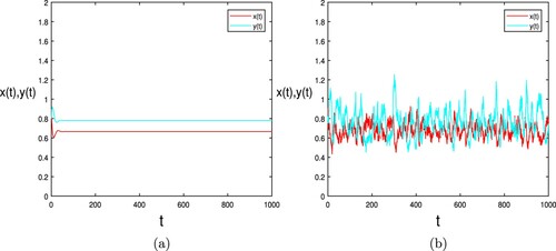In order to show the effect of white noise on population $x\left(t\right)$ and $y\left(t\right)$, we respectively take ${\sigma }_1={\sigma }_2=0$ and ${\sigma }_1=0.05,{\sigma }_2=0.05$, as shown in Figure 1(a,b).

Figure 1. Numerical simulation of the deterministic model (2(2) $\begin{array}{rl}& \frac{\mathrm{d}x}{\mathrm{d}t}=x\left(r-\frac{rx}{K}-by\right),\\ & \frac{\mathrm{d}y}{\mathrm{d}t}=y\left(\frac{\lambda bx}{1+bhx}-d_1\right).\end{array}$(2) ) and stochastic system (3(3) $\begin{array}{rl}\mathrm{d}x& =x\left(r-\frac{rx}{K}-by\right)\mathrm{d}t+{\sigma }_{1}x\mathrm{d}{B}_1\left(t\right),\\ \mathrm{d}y& =y\left(\frac{\lambda bx}{1+bhx}-d_1\right)\mathrm{d}t+{\sigma }_{2}y\mathrm{d}{B}_2\left(t\right),\end{array}$(3) ) with ${\sigma }_1={\sigma }_2=0.05$ respectively are shown in (a) and (b), where the initial value $\left(x\right(0),y(0\left)\right)=(0.9,0.8)$ and other parameters are taken as (10(10) $r=0.4,K=1.3,\lambda =1.3,b=0.25,h=0.5,d_1=\mathrm{0.2.}$(10) ).

In addition, let ${\sigma }_1={\sigma }_2=0.1$ and other values are the same as (10(10) $r=0.4,K=1.3,\lambda =1.3,b=0.25,h=0.5,d_1=\mathrm{0.2.}$(10) ). The calculation predicts that $1+bh{x}^{\ast }-\lambda x^{\ast }\approx 0.2167\ge 0$ and $(\frac{r}{K}-b{y}^{\ast }-{\sigma }_1^2-\frac{l_{1}b}{2}+\frac{b{x}^{\ast }}{2})(x^{\ast }{)}^2\approx 0.0364$, $(l_{1}b{x}^{\ast }-l_1^2{\sigma }_2^2-\frac{l_{1}b}{2}+\frac{b{x}^{\ast }}{2})(y^{\ast }{)}^2\approx 0.0675$, $\omega =\frac{{\sigma }_1^2}{2}{x}^{\ast }+\frac{l_1{\sigma }_2^2}{2}{y}^{\ast }+{\sigma }_1^2(x^{\ast }{)}^2+l_1^2{\sigma }_2^2(y^{\ast }{)}^2\approx 0.0161$. Therefore the condition of Theorem 3.2 is satisfied. 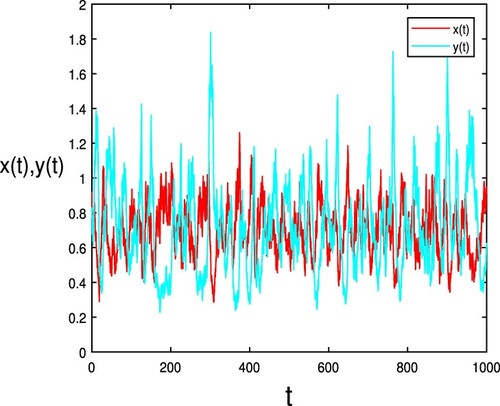So there exists a stationary distribution and it is ergodic in the model (3(3) $\begin{array}{rl}\mathrm{d}x& =x\left(r-\frac{rx}{K}-by\right)\mathrm{d}t+{\sigma }_{1}x\mathrm{d}{B}_1\left(t\right),\\ \mathrm{d}y& =y\left(\frac{\lambda bx}{1+bhx}-d_1\right)\mathrm{d}t+{\sigma }_{2}y\mathrm{d}{B}_2\left(t\right),\end{array}$(3) ) such as Figure 2. When ${\sigma }_1=0.1$, $r-\frac{{\sigma }_1^2}{2}=0.395>0$. Thereby the condition of Theorem 3.3(ii) is established, then the population $x\left(t\right)$ is weakly persistent in the mean almost surely. If the condition keeps unchanged, the population $y\left(t\right)$ is also persistent by simulation. The figures about $x\left(t\right)$ and $y\left(t\right)$ are shown in Figure 3.

Figure 2. Numerical simulation of stationary distribution for the system (3(3) $\begin{array}{rl}\mathrm{d}x& =x\left(r-\frac{rx}{K}-by\right)\mathrm{d}t+{\sigma }_{1}x\mathrm{d}{B}_1\left(t\right),\\ \mathrm{d}y& =y\left(\frac{\lambda bx}{1+bhx}-d_1\right)\mathrm{d}t+{\sigma }_{2}y\mathrm{d}{B}_2\left(t\right),\end{array}$(3) ) with initial value $\left(x\right(0),y(0\left)\right)=(0.9,0.8)$. The parameters are taken as (10(10) $r=0.4,K=1.3,\lambda =1.3,b=0.25,h=0.5,d_1=\mathrm{0.2.}$(10) ) and ${\sigma }_1=0.1,{\sigma }_2=0.1$.

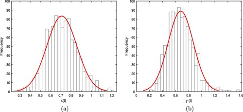
Figure 3. The conditions are exactly the same as the parameters and initial values of Figure 2. The population $x\left(t\right)$ and $y\left(t\right)$ are persistent, where ${\sigma }_1=0.1,{\sigma }_2=0.1$.

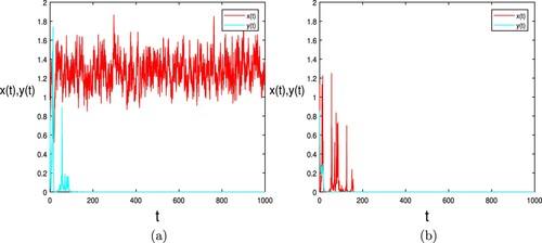
Let ${\sigma }_1=0.1$, ${\sigma }_2=0.7$ and all other parameters keep invariant. By computing, $r-\frac{{\sigma }_1^2}{2}\approx 0.395>0$ and $\lambda bK(r-\frac{{\sigma }_1^2}{2})-r(d_1+\frac{{\sigma }_2^2}{2})=-0.0111<0$, which satisfies the condition of Theorems 3.3(ii) and 3.4. Therefore, the population $x\left(t\right)$ is persistent and $y\left(t\right)$ tent to extinct almost surely. The result is shown in Figure 4(a). By increasing the value of ${\sigma }_1$ so that ${\sigma }_1=0.9$, we give $r-\frac{{\sigma }_1^2}{2}=-0.005<0$. So the condition of Theorem 3.3(i) holds. That is to say, the population $x\left(t\right)$ will go to extinct almost surely. Therefore, we choose ${\sigma }_2=0.2$ and other parameters keep consistent with (10(10) $r=0.4,K=1.3,\lambda =1.3,b=0.25,h=0.5,d_1=\mathrm{0.2.}$(10) ), then $\lambda bK(r-\frac{{\sigma }_1^2}{2})-r(d_1+\frac{{\sigma }_2^2}{2})\approx -0.9011<0$ where the population $x\left(t\right)$ is extinct. Consequently, $y\left(t\right)$ will go to extinct such as Figure 4(b).

Figure 4. In (a), when $x\left(t\right)$ is persistent almost surely and parameters satisfy the condition of Theorem 3.4, the predator $y\left(t\right)$ go to extinct almost surely, where ${\sigma }_1=0.1$, ${\sigma }_2=0.7$ and other values as (10(10) $r=0.4,K=1.3,\lambda =1.3,b=0.25,h=0.5,d_1=\mathrm{0.2.}$(10) ). In (b), when $x\left(t\right)$ tend to extinct almost surely and parameters satisfy the condition of Theorem 3.4, the predator $y\left(t\right)$ go to extinct almost surely, where ${\sigma }_1=0.9$, ${\sigma }_2=0.2$ and other values are the same as (10(10) $r=0.4,K=1.3,\lambda =1.3,b=0.25,h=0.5,d_1=\mathrm{0.2.}$(10) ).

5. Discussion and conclusion

We have considered the influence of the white noise on the model (2(2) $\begin{array}{rl}& \frac{\mathrm{d}x}{\mathrm{d}t}=x\left(r-\frac{rx}{K}-by\right),\\ & \frac{\mathrm{d}y}{\mathrm{d}t}=y\left(\frac{\lambda bx}{1+bhx}-d_1\right).\end{array}$(2) ) in this article. The innovation of the system (2(2) $\begin{array}{rl}& \frac{\mathrm{d}x}{\mathrm{d}t}=x\left(r-\frac{rx}{K}-by\right),\\ & \frac{\mathrm{d}y}{\mathrm{d}t}=y\left(\frac{\lambda bx}{1+bhx}-d_1\right).\end{array}$(2) ) is that it has taken into account the relationship between predation rate of the predator and the density of the prey and consider the effect of the environment capital of the population $x\left(t\right)$. On this basis, due to the disturbance of the environment to the population, we have considered the effect of the noise on predators and prey, which has made our research model (3(3) $\begin{array}{rl}\mathrm{d}x& =x\left(r-\frac{rx}{K}-by\right)\mathrm{d}t+{\sigma }_{1}x\mathrm{d}{B}_1\left(t\right),\\ \mathrm{d}y& =y\left(\frac{\lambda bx}{1+bhx}-d_1\right)\mathrm{d}t+{\sigma }_{2}y\mathrm{d}{B}_2\left(t\right),\end{array}$(3) ) more consistent with the ecological significance.

We have first proved the existence and uniqueness of the global positive solution of the model (3(3) $\begin{array}{rl}\mathrm{d}x& =x\left(r-\frac{rx}{K}-by\right)\mathrm{d}t+{\sigma }_{1}x\mathrm{d}{B}_1\left(t\right),\\ \mathrm{d}y& =y\left(\frac{\lambda bx}{1+bhx}-d_1\right)\mathrm{d}t+{\sigma }_{2}y\mathrm{d}{B}_2\left(t\right),\end{array}$(3) ), which is the prerequisite for studying the long-term behaviour of predators and prey. Under the condition that the positive equilibrium point of system (2(2) $\begin{array}{rl}& \frac{\mathrm{d}x}{\mathrm{d}t}=x\left(r-\frac{rx}{K}-by\right),\\ & \frac{\mathrm{d}y}{\mathrm{d}t}=y\left(\frac{\lambda bx}{1+bhx}-d_1\right).\end{array}$(2) ) exists, we have proved the existence of the stationary distribution and its ergodic property which means the predator and the prey are both permanent.

By the comparison of Figures 1, 3 and 4, we have access to the following conclusion:

1. With the increase of ${\sigma }_1$ and ${\sigma }_2$, the dynamic properties of the system (3(3) $\begin{array}{rl}\mathrm{d}x& =x\left(r-\frac{rx}{K}-by\right)\mathrm{d}t+{\sigma }_{1}x\mathrm{d}{B}_1\left(t\right),\\ \mathrm{d}y& =y\left(\frac{\lambda bx}{1+bhx}-d_1\right)\mathrm{d}t+{\sigma }_{2}y\mathrm{d}{B}_2\left(t\right),\end{array}$(3) ) will also change.

2. White noise has no effect on the system (3(3) $\begin{array}{rl}\mathrm{d}x& =x\left(r-\frac{rx}{K}-by\right)\mathrm{d}t+{\sigma }_{1}x\mathrm{d}{B}_1\left(t\right),\\ \mathrm{d}y& =y\left(\frac{\lambda bx}{1+bhx}-d_1\right)\mathrm{d}t+{\sigma }_{2}y\mathrm{d}{B}_2\left(t\right),\end{array}$(3) ) when ${\sigma }_1={\sigma }_2=0$. But when the values of ${\sigma }_1$ and ${\sigma }_2$ become larger, the perturbation effect of white noise will be more obvious.

3. The population $x\left(t\right)$ will be persistent almost surely if $r-\frac{{\sigma }_1^2}{2}>0$. Under the premise, the population $y\left(t\right)$ will tend to become extinct almost surely if ${\sigma }_2$ is sufficiently large.

4. When ${\sigma }_1$ is sufficiently large, the population $x\left(t\right)$ and $y\left(t\right)$ tend to become extinct almost surely.

Therefore, we make the population extinct by controlling the size of ${\sigma }_1$ and ${\sigma }_2$. From the numerical simulation, under the same conditions, a small white noise will make the system persist. And the larger white noise will make species become extinct. It is also possible to control the size of the disturbance so that the prey lasts and the predator becomes extinct. From our model, when the prey is extinct and the predator has no other source of food, the predator must be extinct.

Acknowledgments

This work was supported by the National Natural Sciences Foundation of China (No. 11971405), Fujian provincial Natural science of China (No. 2018J01418) and National Natural Science Foundation Breeding Program of Jimei University (No. ZP2020064).

Disclosure statement

No potential conflict of interest was reported by the author(s).

Additional information

Funding

This work was supported by the National Natural Sciences Foundation of China [grant number 11971405], Fujian Provincial Natural Science of China [grant number 2018J01418] and National Natural Science Foundation Breeding Program of Jimei University [grant number ZP2020064].

References

- M. Bandyopadhyay, J. Chattopadhyay, Ratio-dependent predator-prey model: Effect of environmental fluctuation and stability, Nonlinearity. 18 (2005), pp. 913–936.
- L.Bellet, Ergodic Properties of Markov Processes In: Attal S., Joye A., Pillet CA. (eds) Open Quantum Systems II, Springer, Berlin, Heidelberg, 2006.
- Y. Cai, Y. Kang, and W. Wang, A stochastic SIRS epidemic model with nonlinear incidence rate, Appl. Math. Comput. 305 (2017), pp. 221–240.
- Y. Cai, J. Jiao, Z. Gui, Y. Liu, and W. Wang, Environmental variability in a stochastic epidemic model, Appl. Math. Comput. 329 (2018), pp. 210–226.
- N. Dalal, D. Greenhalgh, and X. Mao, A stochastic model for internal HIV dynamics, J. Math. Anal. Appl. 341 (2008), pp. 1084–1101.
- R. Durrett, Stochastic Calculus, CRC Press, Boca Raton, 1996.
- A. Farajzadeh, M. Doust, F. Haghighifar, and D. Baleanu, The stability of gauss model having one-prey and two-predators, Abstr. Appl. Anal. 2012 (2012), pp. 1–9.
- X. He and S. Zheng, Protection zone in a diffusive predator-prey model with Beddington-DeAngelis functional response, J. Math. Biol. 75 (2016), pp. 239–257.
- D. Higham, An algorithmic introduction to numerical simulation of stochastic differential equations, SIAM Rev. 43 (2001), pp. 525–546.
- S. Jana and T. Kar, Modeling and analysis of a prey-predator system with disease in the prey, Chaos Soliton. Fract. 47 (2013), pp. 42–53.
- C. Ji and D. Jiang, Analysis of a predator-prey model with disease in the prey, Int. J. Biomath. 6 (2013), p. 1350012.
- C. Ji, D. Jiang, and N. Shi, Analysis of a predator-prey model with modified Leslie–Gower and Holling-type II schemes with stochastic perturbation, J. Math. Anal. Appl. 359 (2009), pp. 482–498.
- J. Jiao, R. Wang, H. Chang, and X. Liu, Codimension bifurcation analysis of a modified Leslie–Gower predator-prey model with two delays, Int. J. Bifurcat. Chaos 28 (2018), p. 1850060.
- B. Kang, B. Liu, and F. Tao, An integrated pest management model with dose-response effect of pesticides, J. Biol. Syst. 26 (2018), pp. 59–86.
- R. Khasminskii, Stochastic Stability of Differential Equations, Sijthoff and Noordhoff, Alphen aan den Rijn, 1980.
- S. Kumar and S. Chattopadh, A bioeconomic model of two equally dominated prey and one predator system, Mod. Appl. Sci. 4 (2010), pp. 84–96.
- G. Lan, Y. Fu, C. Wei, and S. Zhang, Dynamical analysis of a ratio-dependent predator-prey model with Holling III type functional response and nonlinear harvesting in a random environment, Adv. Differ. Equ.-NY 2018 (2018), p. 198.
- S. Li and X. Wang, Analysis of a stochastic predator–prey model with disease in the predator and Beddington–Deangelis functional response, Adv. Differ. Equ.-NY 2015 (2015), p. 224.
- M. Liu, Dynamics of a stochastic regime-switching predator-prey model with modified Leslie–Gower Holling-type II schemes and prey harvesting, Nonlinear Dyn. 96 (2019), pp. 417–442.
- M. Liu and C. Bai, Dynamics of a stochastic one-prey two-predator model with Lévy jumps, J. Comput. Appl. Math. 284 (2016), pp. 308–321.
- Z. Liu and Q. Liu, Persistence and extinction of a stochastic delay predator-prey model under regime switching, Appl. Math.-Czech. 59 (2014), pp. 331–343.
- M. Liu, K. Wang, Persistence and extinction of a stochastic single-species population model in a polluted environment with random perturbations and impulsive toxicant input, Chaos. Soliton. Fract. 45 (2012), pp. 1541–1550.
- M. Liu and K. Wang, Survival analysis of stochastic single-species population models in polluted environments, Ecol. Model. 220 (2009), pp. 1347–1357.
- M. Liu and K. Wang, Persistence and extinction of a stochastic single-specie model under regime switching in a polluted environment, J. Theor. Biol. 264 (2010), pp. 934–944.
- M. Liu and K. Wang, Persistence and extinction in stochastic non-autonomous logistic systems, J. Math. Anal. Appl. 63 (2012), pp. 871–886.
- M. Liu and K. Wang, Persistence and extinction of a single-species population system in a polluted environment with random perturbations and impulsive toxicant input, Chaos Soliton. Fract. 45 (2012), pp. 1541–1550.
- M. Liu and K. Wang, Survival analysis of a stochastic single-species population model with jumps in a polluted environment, Int. J. Biomath. 9 (2016), pp. 207–221.
- M. Liu, K. Wang, and Y. Wang, Long term behaviors of stochastic single-species growth models in a polluted environment, Appl. Math. Model. 35 (2011), pp. 752–762.
- M. Liu, C. Bai, M. Deng, and B. Du, Analysis of stochastic two-prey one-predator model with Lévy jumps, Physica A 445 (2016), pp. 176–188.
- Q. Liu, D. Jiang, T. Hayat, and A. Alsaedi, Dynamics of a stochastic predator–prey model with stage structure for predator and Holling type II functional response, J. Nonlinear Sci. 28 (2018), pp. 1151–1187.
- J. Liu, L. Chen, and F. Wei, The persistence and extinction of a stochastic SIS epidemic model with logistic growth, Adv. Differ. Equ. 2018 (2018), p. 68.
- R. May and N. Macdonald, Stability and complexity in model ecosystems, IEEE Trans. Syst. Man. Cybern. 8 (2007), pp. 779–779.
- L. Nie, J. Peng, Z. Teng, and L. Hu, Existence and stability of periodic solution of a Lotka–Volterra predator-prey model with state dependent impulsive effects, J. Comput. Appl. Math. 224 (2009), pp. 544–555.
- P. Pal, M. Haque, and P. Mandal, Dynamics of a predator–prey model with disease in the predator, Math. Methods Appl. Sci. 37 (2013), pp. 2429–2450.
- P. Pang and M. Wang, Strategy and stationary pattern in a three-species predator–prey model, J. Differ. Equ. 200 (2004), pp. 245–273.
- K. Sun, T. Zhang, and Y. Tian, Dynamics analysis and control optimization of a pest management predator–prey model with an integrated control strategy, Appl. Math. Comput. 292 (2017), pp. 253–271.
- S. Tang, Y. Xiao, L. Chen, and R. Cheke, Integrated pest management models and their dynamical behaviour, Bull. Math. Biol. 67 (2005), pp. 115–135.
- S. Tang, J. Liang, Y. Tan, and R. Cheke, Threshold conditions for integrated pest management models with pesticides that have residual effects, J. Math. Biol. 66 (2013), pp. 1–35.
- Y. Tian, K. Sun, and L. Chen, Comment on existence and stability of periodic solution of a Lotka–Volterra predator–prey model with state dependent impulsive effects, J. Comput. Appl. Math.234 (2010), pp. 2916–2923.
- J. Tripathi, S. Abbas, and M. Thakur, Local and global stability analysis of a two prey one predator model with help, Commun. Nonlinear Sci. 19 (2014), pp. 3284–3297.
- F. Wei and L. Chen, Psychological effect on single-species population models in a polluted environment, Math. Biosci. 290 (2017), pp. 22–30.
- F. Wei, S. Geritz, and J. Cai, A stochastic single-species population model with partial pollution tolerance in a polluted environment, Appl. Math. Lett. 63 (2017), pp. 130–136.
- C. Wei, J. Liu, and S. Zhang, Analysis of a stochastic eco-epidemiological model with modified Leslie–Gower functional response, Adv. Differ. Equ. 2018 (2018), p. 119.
- Z. Xiang, S. Tang, C. Xiang, and J. Wu, On impulsive pest control using integrated intervention strategies, Appl. Math. Comput. 269 (2015), pp. 930–946.
- Y. Xiao and L. Chen, Modeling and analysis of a predator–prey model with disease in the prey, Math. Biosci. 171 (2001), pp. 59–82.
- R. Xu and S. Zhang, Modelling and analysis of a delayed predator–prey model with disease in the predator, Appl. Math. Comput. 224 (2013), pp. 372–386.
- X. Yu, S. Yuan, and T. Zhang, The effects of toxin-producing phytoplankton and environmental fluctuations on the planktonic blooms, Nonlinear Dyn. 91 (2018), pp. 1653–1668.
- C. Zhu and G. Yin, On competitive Lotka–Volterra model in random environments, J. Math. Anal. Appl. 357 (2009), pp. 154–170.