A discrete/continuous time resource competition model and its implications

Abstract

We use a mixed time model to study the dynamics of a system consisting of two consumers that reproduce only in annual birth pulses, possibly at different times, with interaction limited to competition for a resource that reproduces continuously. Ecological theory predicts competitive exclusion; this expectation is met under most circumstances, the winner being the species with the greater ‘power’, defined as the time average consumer level at the fixed point. Instability of that fixed point for the stronger competitor slightly weakens its domination, so that a resident species with an unstable fixed point can sometimes be invaded by a slightly weaker species, leading ultimately to coexistence. Differences in birth pulse times can lead to qualitatively different long-term coexistence behaviour, including cycles of different lengths or chaos. We also determine conditions under which the timing of an annual pulse of a toxin can change the balance of power.

Keywords:

• Population dynamics
• competition
• mixed time models
• toxic effects
• stability

1. Introduction

In this paper, we study the dynamics of a population model for two consumers competing for a single resource. We assume that the resource is governed by an ordinary differential equation describing continuous growth and reproduction, while the consumer stores resources for reproduction at birth pulses at a regular time interval. The dynamic model tracks the levels of the resource and the consumers using a discrete model for integer time steps, representing a census point in each year along with a continuous model to describe the changes during the year. We therefore use:

• A discrete model that tracks resource level and consumer populations at an annual census, with

• An embedded continuous model that tracks resource levels and consumer populations during the time between census events.

In our model the competition between consumer species consists strictly of competition for resource collection, which is called exploitative competition. We assume that there is no interference competition; that is, neither species directly affects the other's birth and death rates. A general discussion of the differences between exploitative and interference competition can be found in [5]. Our assumptions on the type of competition present have significant consequences for the behaviour of the system.

The model in this paper is based on the model in Pachepsky et al. [12], which has a resource, a single consumer, and a birth pulse. Our model incorporates a second consumer competing for the resource. For a general discussion of consumer–resource models, see [9]. There are many population models incorporating a birth pulse, including [1–4, 6, 11, 14]. This type of model is sometimes called semi-discrete, and is the subject of the survey [8]. Competition models with birth pulses and interference competition can be found in [1, 3, 4, 6]. Models with exploitative competition can be found in [5, 10, 15]. We are unaware of any competition models in the literature incorporating birth pulses and exploitative competition.

In Section 2, we study the dynamics of the model with a resource and a single consumer. This was analysed in [12], but a reworking and extension of their results are needed to facilitate the analysis of the two-consumer model.

The model with two consumers competing for one resource is given in Section 3. We include in the model the possibility that the birth pulses for the two consumers occur at different times in the annual cycle.

In Section 3.1, we give some mathematical results about the possibilities of co-existence of the two consumers. Proposition 3.1 gives a very stringent condition for there to be a fixed point with the mutual survival of the two consumers. When one consumer is a resident and the other is an invader, Proposition 3.2 gives a natural condition for when the invasion will be successful. These results are independent of the timing of the birth pulses.

The mathematical results in Section 3.1 do not cover all cases that are possible in the competition model. In Section 4, we use simulations to examine invasions and long-term dynamics in these other cases.

Finally, in Section 5, we consider a hypothetical example where two fish species competing for the same resource are subjected to a toxin dumped once a year into their habitat. It has been observed in the literature [1, 6, 7] that if a stressor is applied to a competition system, the resulting change in life history in both competitors can help the weaker competitor. We will use our model to show how this can occur in a competition model of the form considered in this paper. Whether or not this happens depends upon the relationship between the timing of the birth pulses and the timing of the toxin release. For a more extensive analysis (via simulations) of the effect of timing on consumer–resource systems, see [13].

2. Mixed time consumer–resource model

We first study the dynamics of a single consumer and a resource. While a large part of this analysis is in [12], we present the key elements here because a shared notation and understanding of the single-consumer system is a prerequisite to presentation of the dynamics when there are two consumers.

A mixed time model consists of a continuous-time system embedded in a discrete system. We take the initial state to be at discrete time t = 0. For convenience, we label the initial year as ‘year 0’. The dynamics of year 0 uses a continuous-time variable $0\le s\le 1$. A birth pulse occurs at the very end of the year, creating a discontinuity in the consumer population between continuous-time s = 1 and discrete-time t = 1. In subsequent years, the values of the dependent variables at discrete time t serve as initial conditions for that year's continuous model, and the consumer and resource levels for year t + 1 result from the levels at continuous time s = 1, with the consumer level augmented by the end-of-year birth pulse.

Let F be the biomass of a resource and let X be the population of a consumer. Let $U_t$ and $V_t$ be the resource level and consumer population at the beginning of year t, taking the initial year to be year 0.

Table 1 summarizes the dependent and independent variables in the two time regimes.

Table 1. Notation for the dependent and independent variables in the continuous and discrete time regimes.

	Continuous	Discrete
Time	$0\le s\le 1$	$t=0,1,\dots$
Resource Biomass	$F(s)$	$U_t$
Consumer Population	$X(s)$	$V_t$

The $(U,V)$ system is defined by a discrete map $U_{t+1}=P(U_t,V_t);V_{t+1}=Q(U_t,V_t),$along with initial states $U_0$ and $V_0$, where the functions P and Q are determined by the continuous dynamics of year t, consisting of the continuous dynamics plus the end-of-year birth pulse.

The continuous model must track the resource level F, the consumer population X, and the cumulative resource acquisition per consumer b over the time interval represented by continuous-time $0\le s\le 1$ and discrete-time $(t,t+1)$. The processes that impact these quantities are logistic growth of vegetation, with growth rate ρ and carrying capacity K, natural death of the consumers with rate constant μ, and consumption at a rate aFX. The choice of a consumption rate model without density dependence corresponds to the assumption that actual resource levels F are far below the resource level required for consumer satiation. We take b to be measured in units of future consumers, so that its value at the end of the continuous regime is the number of newborn consumers per adult consumer without need of an additional parameter. With these quantities and processes, the system in the continuous regime of year t is given by (1) $\begin{array}{rl}\frac{\mathrm{d}F}{\mathrm{d}s}& =\rho F(1-\frac{F}{K})-aFX;\end{array}$(1) (2) $\begin{array}{rl}\frac{\mathrm{d}X}{\mathrm{d}s}& =-\mu X;\end{array}$(2) (3) $\begin{array}{rl}\frac{\mathrm{d}b}{\mathrm{d}s}& =\theta aF,\end{array}$(3) where θ is the number of offspring that are produced from one unit of resource consumption.

The continuous model is embedded in the discrete model by associating initial and terminal conditions to levels recorded at the relevant census. At the beginning of each continuous period, levels of resource and consumer are those measured at time t, while the initial resource accumulation is 0: (4) $F(0)=U_t,X(0)=V_t,b(0)=0.$(4) At the end of the continuous period, the resource and consumer levels carry over, while the acquired resources are converted into new consumers: (5) $U_{t+1}=F(1),V_{t+1}=[1+b(1)]X(1),$(5) where the population of new consumers is the product of the number of those consumers and the average number of offspring of those consumers.

For nondimensionalization, we first note that the resource acquisition level b and the time s are dimensionless by design; thus the parameters μ and ρ are already dimensionless. In addition to the resource and consumer levels, the parameters K, a, and θ are not dimensionless, with K a resource biomass, a in 1/consumer and θ in consumers/resource biomass. We nondimensionalize the model by introducing dimensionless quantities with lower-case letters corresponding to the capital letters used for the dimensional version and combining the three dimensional parameters into a single dimensionless combination: (6) $f=\frac{F}{K},x=\frac{aX}{\rho },u=\frac{U}{K},v=\frac{aV}{\rho },\alpha =\theta aK.$(6) The scale $\rho /a$ chosen for the consumer represents the population size that can be achieved if the resource grows at maximum rate $\rho F$. In a continuous model, this would guarantee f, x, u, v<1; these restrictions will not apply here because the resources accumulated by the consumer during the year only begin to affect the consumer population after the birth pulse. With these dimensionless quantities, the model becomes (7) $\begin{array}{rl}\frac{\mathrm{d}f}{\mathrm{d}s}& =\rho f(1-f-x),f(0)=u_t,u_{t+1}=f(1);\end{array}$(7) (8) $\begin{array}{rl}\frac{\mathrm{d}x}{\mathrm{d}s}& =-\mu x,x(0)=v_t,v_{t+1}=[1+b(1)]x(1);\end{array}$(8) (9) $\begin{array}{rl}\frac{\mathrm{d}b}{\mathrm{d}s}& =\alpha f,b(0)=0.\end{array}$(9)

The continuous model is embedded in the discrete model; that is, its use is merely to determine the map from time t to time t + 1. We, therefore, focus on the discrete map, its fixed points, and their stability. Simulation graphs will show the levels at the census times, which come just after the birth pulse (as seen in the last equation of (8(8) $\begin{array}{rl}\frac{\mathrm{d}x}{\mathrm{d}s}& =-\mu x,x(0)=v_t,v_{t+1}=[1+b(1)]x(1);\end{array}$(8) )).

In the absence of consumers, the model reduces to the logistic equation for the resource, so the fixed point at U = 1, V = 0 needs only be checked for stability with respect to an initial perturbation in the consumer population. Therefore, we assume that the consumer is introduced at a very low level $v_0>0$, so the continuous-time problem over each time step for x reduces to $\frac{\mathrm{d}x}{\mathrm{d}s}=-\mu x,x(0)=v_0\ll 1,v_1=[1+b(1)]x(1).$Here, $b(1)={\int }_0^1\alpha f(s)\mathrm{d}s\sim \alpha [1-O(v_0)],$which follows from the fact that an $O(v_0)$ perturbation in the consumer population creates a perturbation of the same size in the resource level; hence $f(s)=1-O(v_0)$, and similarly for the integral of f. Note that the presence of a small consumer population decreases the resource level; hence, the $O(v_0)$ perturbations in f and b are necessarily positive with the minus signs as written. Consumer persistence occurs if and only if $v_1/v_0\ge 1$. Since $v_1=(1+\alpha )v_0{\mathrm{e}}^{-\mu }-O(v_0^2)$, with the perturbation again positive as written, we see that this happens if and only if (10) $(\alpha +1){\mathrm{e}}^{-\mu }>1.$(10) Thus (10(10) $(\alpha +1){\mathrm{e}}^{-\mu }>1.$(10) ) is a necessary and sufficient condition for persistence of the consumer. In the sequel, we assume this condition holds.

We now study the coexistence equilibrium. We will see that in the case where it is stable, the most important features are the mean resource and consumer levels corresponding to the fixed point, rather than the fixed point itself. We denote these as $\overline{f}$ and $\overline{x}$, respectively. These quantities can be computed from (7(7) $\begin{array}{rl}\frac{\mathrm{d}f}{\mathrm{d}s}& =\rho f(1-f-x),f(0)=u_t,u_{t+1}=f(1);\end{array}$(7) )–(9(9) $\begin{array}{rl}\frac{\mathrm{d}b}{\mathrm{d}s}& =\alpha f,b(0)=0.\end{array}$(9) ). For convenience, denote $z=1+b(1).$Using (8(8) $\begin{array}{rl}\frac{\mathrm{d}x}{\mathrm{d}s}& =-\mu x,x(0)=v_t,v_{t+1}=[1+b(1)]x(1);\end{array}$(8) ) at a fixed point $v_t=v^{\ast }$, we have $v_t=v_{t+1}=zx(1)=z{v}_t{\mathrm{e}}^{-\mu };$hence, $z={\mathrm{e}}^{\mu }$ and so $b(1)={\mathrm{e}}^{\mu }-1$. Integrating (9(9) $\begin{array}{rl}\frac{\mathrm{d}b}{\mathrm{d}s}& =\alpha f,b(0)=0.\end{array}$(9) ) from 0 to 1 yields $b(1)=\alpha {\int }_0^{1}f(s)\mathrm{d}s=\alpha \overline{f},$with the result (using the standing assumption (10(10) $(\alpha +1){\mathrm{e}}^{-\mu }>1.$(10) )) (11) $\overline{f}=\frac{{\mathrm{e}}^{\mu }-1}{\alpha }<1.$(11) Returning to (7(7) $\begin{array}{rl}\frac{\mathrm{d}f}{\mathrm{d}s}& =\rho f(1-f-x),f(0)=u_t,u_{t+1}=f(1);\end{array}$(7) ), we divide both sides by $\rho f$ and then integrate from 0 to 1 to get $1-\overline{f}-\overline{x}={\frac{1}{\rho }\ln f|}_{s=0}^1=0,$from which we obtain (12) $\overline{x}=1-\overline{f}<1.$(12) The values of 1 in the inequalities of (11(11) $\overline{f}=\frac{{\mathrm{e}}^{\mu }-1}{\alpha }<1.$(11) ) and (12(12) $\overline{x}=1-\overline{f}<1.$(12) ) are least upper bounds, confirming that the scales chosen for F and X in (6(6) $f=\frac{F}{K},x=\frac{aX}{\rho },u=\frac{U}{K},v=\frac{aV}{\rho },\alpha =\theta aK.$(6) ) correspond to the maximum equilibrium values for these quantities. Note that $\overline{f}$ and $\overline{x}$ cannot be interpreted as the annual means when the fixed point is unstable; however, we will still find the formulas in those equations to have value in the competition model.

The fixed point $(u^{\ast },v^{\ast })$ of (7(7) $\begin{array}{rl}\frac{\mathrm{d}f}{\mathrm{d}s}& =\rho f(1-f-x),f(0)=u_t,u_{t+1}=f(1);\end{array}$(7) )–(9(9) $\begin{array}{rl}\frac{\mathrm{d}b}{\mathrm{d}s}& =\alpha f,b(0)=0.\end{array}$(9) ) is given by (see the Appendix for details) (13) $v^{\ast }=\frac{{\mathrm{e}}^{\mu }M}{A},u^{\ast }=\frac{1-\delta }{\rho \delta I},$(13) where (14) $A=\frac{\alpha (1-{\mathrm{e}}^{-\mu })}{\mu }>0,M=(\alpha +1){\mathrm{e}}^{-\mu }-1>0,\delta ={\mathrm{e}}^{-\rho \overline{f}}$(14) and (15) $I={\int }_0^1{G}^{\ast }(s)\mathrm{d}s,G^{\ast }(s)=\exp (\rho s-\rho \overline{x}\frac{1-{\mathrm{e}}^{-\mu s}}{1-{\mathrm{e}}^{-\mu }}).$(15) The necessary and sufficient conditions for asymptotic stability of this fixed point are shown in the Appendix to be (16) $\frac{1}{M}>1-q,\frac{1}{M}>\frac{1-\delta }{1+\delta }(q-\frac{1}{2}),$(16) where (17) $q=\frac{{\int }_0^1(1-{\mathrm{e}}^{-\mu s})G^{\ast }(s)\mathrm{d}s}{{\int }_0^1(1-{\mathrm{e}}^{-\mu })G^{\ast }(s)\mathrm{d}s}.$(17) These are equivalent to those in [12], but much easier to evaluate.

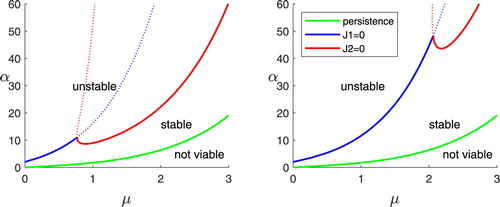
Figure 1 shows bifurcation diagrams in the μ-α parameter space for two values of ρ. When μ is fixed, the value of α determines whether the coexistence equilibrium is unstable, stable, or not viable. The stability boundary is a piecewise-continuous curve, in which the left portion, which we call the $J_1$ instability, is where the first inequality of (16(16) $\frac{1}{M}>1-q,\frac{1}{M}>\frac{1-\delta }{1+\delta }(q-\frac{1}{2}),$(16) ) is violated, while the right portion, or $J_2$ instability, is determined by the second inequality of (16(16) $\frac{1}{M}>1-q,\frac{1}{M}>\frac{1-\delta }{1+\delta }(q-\frac{1}{2}),$(16) ).

Figure 1. Bifurcation diagrams in the $\mu \alpha$ parameter space. (a) $\rho =20$ fast resource growth. (b) $\rho =10$ moderate resource growth

Figures 2 and 3 show behaviours for sequences of points in the μ-α parameter space with $\rho =20$, one sequence for each of the two boundaries. One approach to creating these plots is to fix μ and choose a sequence of increasing α values. In anticipation of the theory of competition developed in the following section, we have chosen instead to fix the value of $\overline{x}$, choose a sequence of increasing μ values, and calculate the corresponding α values from (11(11) $\overline{f}=\frac{{\mathrm{e}}^{\mu }-1}{\alpha }<1.$(11) ) and (12(12) $\overline{x}=1-\overline{f}<1.$(12) ). The $J_2$ instability is explored with a sequence of points having $\overline{x}=0.84$ (Figure 2) and the $J_1$ instability with a sequence having $\overline{x}=0.92$ (Figure 3). In both cases, simulations were done using initial conditions close to the unstable fixed point and run long enough for a clear pattern to develop. The different cases are marked in the left half of the figure by points in the $\mu \alpha$ plane, and the corresponding results are shown in a stack of plots in the right half of the figure, arranged from the highest value of α down to lowest so that the vertical ordering of the plots matches the vertical ordering of the points.

Figure 2. Discrete map trajectories with $\overline{x}=0.84$ and μ values of 1.0, 1.3, 1.6, 1.9, and 2.2 (bottom to top); the left panel locates the five points in the parameter space.

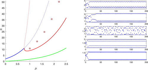
Figure 3. Discrete map trajectories with $\overline{x}=0.92$ and μ values of 0.325, 0.35, 0.375, 0.425, and 0.5 (bottom to top); the left panel locates the five points in the parameter space.

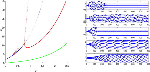
We see in Figures 2 and 3 that the behaviour in the unstable range depends on which stability boundary is crossed. The $J_2$ stability boundary behaves like the discrete logistic map, with period-doubling that leads to a combination of chaos for some points and limit cycles of unusual period for others, in this case including a 3-cycle for $\mu =1.9$ and a 7-cycle for $\mu =2.2$. This is referred to in [12] as overcompensation. For the $J_1$ stability boundary, any possible period-doubling could only occur in a very narrow band. The simulations show a variety of unpredictable behaviours. Moving away from the stability boundary, we see a cycle with some indeterminate large period at $\mu =0.325$, a 101-cycle at $\mu =0.35$, a 7-cycle at $\mu =0.375$, chaos at $\mu =0.425$, and a 3-cycle at $\mu =0.5$. Pachepsky et al. [12] describes this as a region of consumer–resource cycles, but because of the chaotic behaviour for some points, it is more accurately described as consumer–resource instability.

3. Resource competition model

Let F be the biomass of a common resource and let X and Y be the populations of two different consumers. Let $U_t$ be the resource level at the beginning of year t, and let $V_t$ and $W_t$ be the consumer populations (associated with X and Y, respectively), also at the beginning of year t. As in the consumer–resource model above, we assume that F experiences continuous growth and reproduction, while the consumers store resources for reproduction in birth pulses at possibly different times. Once again, the dynamic model tracks the levels of the resource and the consumer using a discrete model for integer time steps $t=0,1,2,\dots$, representing a census point in each year, along with a continuous model to describe the changes during the year. We assume without loss of generality that the X population's birth pulses are at the census points $1,2,\dots$, and that the Y population has birth pulses at $\tau ,1+\tau ,2+\tau ,\dots$ for a fixed $\tau \in [0,1)$. For a function ϕ and a scalar ν, we use the notation $\varphi ({\nu }^{-})$ to denote the left-sided limit $\underset{s\to {\nu }^{-}}{lim}\varphi (s)$. We will use the notation $\varphi ({\nu }^{+})$ to denote the right-sided limit. (18) $\begin{array}{rl}\frac{\mathrm{d}F}{\mathrm{d}s}& =\rho F(1-\frac{F}{K})-a_{1}FX-a_{2}FY,F(0)=U_t,U_{t+1}=F(1);\end{array}$(18) (19) $\begin{array}{rl}\frac{\mathrm{d}X}{\mathrm{d}s}& =-{\mu }_{1}X,X(0)=V_t,V_{t+1}=z_{1}X(1);\end{array}$(19) (20) $\begin{array}{rl}\frac{\mathrm{d}Y}{\mathrm{d}s}& =-{\mu }_{2}Y,Y(0)=W_t,Y({\tau }^{+})=z_{2}Y({\tau }^{-}),W_{t+1}=Y(1);\end{array}$(20) (21) $\begin{array}{rl}\frac{\mathrm{d}{b}_1}{\mathrm{d}s}& ={\theta }_1{a}_{1}F,b_1(0)=0;\end{array}$(21) (22) $\begin{array}{rl}\frac{\mathrm{d}{b}_2}{\mathrm{d}s}& ={\theta }_2{a}_{2}F,b_2(0)=b_0,b_2({\tau }^{+})=0,b_0=b_2(1);\end{array}$(22) (23) $\begin{array}{rl}{z}_1& =1+b_1(1^{-}),z_2=1+b_2({\tau }^{-}).\end{array}$(23) The variables $b_1$ and $b_2$ represent the amount of resources stored by each individual consumer since the most recent reproductive period, ${\theta }_1$ and ${\theta }_2$ are the number of offspring by each individual consumer that can be produced from one unit of resource consumption. The stored resources for consumer Y are carried over from one year to the next; that is, each year starts where the previous year ended. In the initial year, we take $b_0$ to be specified as part of the scenario. The factors $z_1$ and $z_2$ are introduced for convenience to represent the multiplicative factor by which the respective populations increase through a birth pulse. The linear functions $a_{1}FX$ and $a_{2}FY$ reflect the assumption that the maximum resource level F = K is far below the level required for satiation, else we would need a nonlinear functional response. The consumer populations are subject to natural death during the continuous year, where ${\mu }_i$ are the death rates.

As with the single consumer model, we nondimensionalize this model by introducing dimensionless quantities with lower-case letters: (24) $f=\frac{F}{K},x=\frac{a_{1}X}{\rho },y=\frac{a_{2}Y}{\rho },u=\frac{U}{K},v=\frac{a_{1}V}{\rho },w=\frac{a_{2}W}{\rho },{\alpha }_j={\theta }_j{a}_{j}K.$(24) The choices of scales and the implication of these choices is the same as for the single consumer model.

With the introduction of dimensionless variables, the model becomes (25) $\begin{array}{rl}\frac{\mathrm{d}f}{\mathrm{d}s}& =\rho f(1-f-x-y),f(0)=u_t,u_{t+1}=f(1);\end{array}$(25) (26) $\begin{array}{rl}\frac{\mathrm{d}x}{\mathrm{d}s}& =-{\mu }_{1}x,x(0)=v_t,v_{t+1}=z_{1}x(1);\end{array}$(26) (27) $\begin{array}{rl}\frac{\mathrm{d}y}{\mathrm{d}s}& =-{\mu }_{2}y,y(0)=w_t,y({\tau }^{+})=z_{2}y({\tau }^{-}),w_{t+1}=y(1);\end{array}$(27) (28) $\begin{array}{rl}\frac{\mathrm{d}{b}_1}{\mathrm{d}s}& ={\alpha }_{1}f,b_1(0)=0;\end{array}$(28) (29) $\begin{array}{rl}\frac{\mathrm{d}{b}_2}{\mathrm{d}s}& ={\alpha }_{2}f,b_2(0)=b_0,b_2({\tau }^{+})=0,b_0=b_2(1);\end{array}$(29) (30) $\begin{array}{rl}{z}_1& =1+b_1(1),z_2=1+b_2({\tau }^{-}).\end{array}$(30)

3.1. Analysis of the competition model

Given that the competition in (25(25) $\begin{array}{rl}\frac{\mathrm{d}f}{\mathrm{d}s}& =\rho f(1-f-x-y),f(0)=u_t,u_{t+1}=f(1);\end{array}$(25) )–(30(30) $\begin{array}{rl}{z}_1& =1+b_1(1),z_2=1+b_2({\tau }^{-}).\end{array}$(30) ) is strictly exploitative, the consumers occupy the same ecological niche; hence, ecological theory predicts that the principle of competitive exclusion should hold. Our primary interest in the analysis of the model is to test this prediction. To facilitate the analysis, we define the ‘power’ of a consumer species by (31) $P_i=1-\frac{{\mathrm{e}}^{\mu {}_i}-1}{{\alpha }_i},i=1,2,$(31) where $P_1$ and $P_2$ are the respective powers of population X and Y. This definition is motivated by the single consumer result, where the average consumer level is P and the average resource level is 1−P. Using the symbol P for the power (rather than $\overline{x}$) helps avoid confusion between results for the single consumer model when stable (see (12(12) $\overline{x}=1-\overline{f}<1.$(12) )) and any as yet undetermined results for the competition model. Also note that the viability requirement (10(10) $(\alpha +1){\mathrm{e}}^{-\mu }>1.$(10) ) is equivalent to P>0.

Proposition 3.1

There are no fixed points with mutual survival of consumers 1 and 2 unless (32) $P_1=P_2>0.$(32)

Proof.

Let $\overline{f}$ denote the average of f over any one-year period. If $P_j\le 0$, then the jth consumer is not viable even without competition from the other; hence, a mutual survival fixed point must have $P_j>0$. Now suppose a fixed point $(u^{\ast },v^{\ast },w^{\ast })$ has $v^{\ast }>0$ and $w^{\ast }>0$. Then $1=\frac{v_{t+1}}{v_t}=\frac{z_{1}x(1)}{v_t}=[1+b_1(1)]{\mathrm{e}}^{-{\mu }_1}={\mathrm{e}}^{-{\mu }_1}(1+{\alpha }_1\overline{f});$hence, $\overline{f}=\frac{{\mathrm{e}}^{{\mu }_1}-1}{{\alpha }_1}=1-P_1.$The same calculation yields the result $\overline{f}=\frac{{\mathrm{e}}^{{\mu }_2}-1}{{\alpha }_2}=1-P_2.$Since $\overline{f}$ applies to the full system rather than separately for each consumer, the conclusion (32(32) $P_1=P_2>0.$(32) ) must follow.

Some care is required to interpret the meaning of this proposition. Since the line $P_1=P_2$ has measure 0 in the $(P_1,P_2)$ space, the probability of there being an equilibrium where both consumers survive is zero. This argument assumes that the parameters $P_1$ and $P_2$ are independent. They could still be equal in settings with a biological mechanism that links the parameters so as to dictate equality. Note that this result does not exclude the possibility of mutual consumer survival, although it limits the dynamics of such a scenario by ruling out a stable fixed point.

Proposition 3.2

Suppose the system begins at $(u(0),v(0),w(0))=(u^{\ast },v^{\ast },0)$, where $(u^{\ast },v^{\ast })$ is an asymptotically stable fixed point for the resource and first consumer X. The second consumer Y can successfully invade if and only if its power is greater than that of the resident.

A useful way of looking at this Proposition is that an invasion succeeds when the resource level with which the invader can coexist at steady-state is less than the steady-state resource level of the resident system.

Proof.

Consider (25(25) $\begin{array}{rl}\frac{\mathrm{d}f}{\mathrm{d}s}& =\rho f(1-f-x-y),f(0)=u_t,u_{t+1}=f(1);\end{array}$(25) )–(30(30) $\begin{array}{rl}{z}_1& =1+b_1(1),z_2=1+b_2({\tau }^{-}).\end{array}$(30) ) initially at the fixed point $(u^{\ast },v^{\ast },0)$, with the second consumer introduced through an impulse $y({\tau }^{+})=ϵ$. From (27(27) $\begin{array}{rl}\frac{\mathrm{d}y}{\mathrm{d}s}& =-{\mu }_{2}y,y(0)=w_t,y({\tau }^{+})=z_{2}y({\tau }^{-}),w_{t+1}=y(1);\end{array}$(27) ), we have $y(1+{\tau }^{-})=ϵ{\mathrm{e}}^{-{\mu }_2}$. In the limit as $ϵ\to 0$, the presence of the invader does not change the levels of the resource or the resident consumer; hence, $\overline{f}$ is given by (11(11) $\overline{f}=\frac{{\mathrm{e}}^{\mu }-1}{\alpha }<1.$(11) ) up to a negative $O(ϵ)$ error. Then (29(29) $\begin{array}{rl}\frac{\mathrm{d}{b}_2}{\mathrm{d}s}& ={\alpha }_{2}f,b_2(0)=b_0,b_2({\tau }^{+})=0,b_0=b_2(1);\end{array}$(29) ) yields $b_2(1+{\tau }^{-})={\alpha }_2{\int }_{\tau }^{1+\tau }f\mathrm{d}s={\alpha }_2\overline{f}$up to $O(ϵ)$, and so $y(1+{\tau }^{+})=[1+b_2(1+{\tau }^{-})]y(1+{\tau }^{-})=ϵ{\mathrm{e}}^{-{\mu }_2}(1+{\alpha }_2\overline{f})-O({ϵ}^2).$In the limit $ϵ\to 0$, this quantity is at least as large as $y({\tau }^{+})$ if and only if $1+{\alpha }_2\overline{f}>{\mathrm{e}}^{{\mu }_2}$or $\frac{{\mathrm{e}}^{{\mu }_2}-1}{{\alpha }_2}<\overline{f}=\frac{{\mathrm{e}}^{{\mu }_1}-1}{{\alpha }_1}.$Thus, the invading population increases if and only if $P_2>P_1$.

Note that it is possible for one species to have the greater power even though the other has a greater basic reproductive number, given by $R_0=\frac{1+\alpha }{\mu }.$If both species are introduced into a resource-only environment, the one with the larger basic reproductive number will grow faster initially, but the one with the larger power will ultimately win out. We will see an example of this in Section 4.

Corollary 3.1

Suppose an invader has a stable single-consumer fixed point, and the resident has greater power than the invader. Then the resident will persist.

Proof.

Assume the hypotheses in the statement of the Corollary. Suppose the system (25(25) $\begin{array}{rl}\frac{\mathrm{d}f}{\mathrm{d}s}& =\rho f(1-f-x-y),f(0)=u_t,u_{t+1}=f(1);\end{array}$(25) )–(30(30) $\begin{array}{rl}{z}_1& =1+b_1(1),z_2=1+b_2({\tau }^{-}).\end{array}$(30) ) is initially at some value $(u,v,0)$ and the second consumer is introduced with $y({\tau }^{+})=ϵ$ for small $ϵ>0$. Suppose further that the resident consumer becomes arbitrarily small, in which case the presence of resident does not affect the resource or the invader. In this case (because the invader has a stable single-consumer fixed point), the system consisting of the invader and the resource approaches a stable fixed point $(u^{\ast },w^{\ast })$. However, Proposition 3.2, with the roles of the invader and resident reversed, implies that the former resident, with its greater power, would successfully ‘invade’ this system, which means that the resident will persist. This is a contradiction, so the resident cannot become arbitrarily small.

4. Simulations of competition dynamics

We consider the results of competition for scenarios with a resident species, initially present at its (possibly unstable) equilibrium value, and an invader species, which has a small initial presence.

Table 2 shows the results for all possible combinations of whether the species with a higher power is resident or invader and which, if any, consumer(s) has a stable equilibrium in the absence of competition.

Table 2. Outcomes of an invasion, depending on species power ($P_i$) and stability of single-consumer equilibria.

	Higher power	Stable equilibrium	Invasion successful?	Resident persists?
1	Resident	Resident	NO (Prop. 2)	YES (Prop. 2)
2	Resident	Resident, invader	NO (Prop. 2)	YES (Prop. 2)
3	Resident	None	–	Yes
4	Resident	Invader	Sometimes	YES (Cor. 1)
5	Invader	Invader	Yes	No
6	Invader	Invader, resident	YES (Prop. 2)	No
7	Invader	None	Yes	–
8	Invader	Resident	YES (Prop. 2)	Sometimes

Mathematical results are reported in bold, and observations from simulations are italicized.

We show in column 3 whether or not the invasion is successful, and if this conclusion follows from a mathematical result from Section 3.1. In column 4, we show whether or not the resident persists.

We first briefly discuss the cases where the mathematical results are relevant:

• Rows 1 and 2: The resident has the higher power and a stable equilibrium; hence, Proposition 3.2 is definitive: invasion is not successful and the single-consumer result for the resident applies.

• Row 4: The persistence of the resident follows directly from Corollary 3.1.

• Rows 6 and 8: The stronger competitor is able to invade a stable resident by Proposition 3.2.

We still need to investigate the cases where mathematics is not complete. We will do this via simulations. Unless otherwise stated, we assume that $\tau =1$, that is, the two populations have birth pulses at the same time. We will only show the population at the census points. In the figures, we will only show the resident population, since the invader will have the same type of dynamics.

We now explore the case in row 4, where the resident is stronger, but the invader has a stable equilibrium in the absence of competition. There appears to be a considerable variety of possible behaviours, as illustrated by three examples. In each plot, we show only the resident, as a changed resident behaviour is sufficient evidence of a successful invasion. Additionally, if the invader is successful, its asymptotic behaviour is qualitatively similar (cycle of a specific period or chaos) to that of the resident.

• The system shown in Figure 4 has a 2-cycle in the absence of an invader. With an invader whose power is only slightly less than that of the resident, the 2-cycle structure is maintained, but with yearly resident population values that depend on the timing of the invader's birth pulse.

• The system shown in Figure 5 exhibits chaos in the absence of an invader. With an invader slightly weaker than the resident, the behaviour depends qualitatively on the timing of the birth pulse. Experiments show a 3-cycle when $\tau =1$, a 10 cycle when $\tau =.1$, a 7-cycle when $\tau =.2$, a 13-cycle when $\tau =.95$, and chaos with amplitudes restricted by an envelope for those τ values we tried in the range from 0.3 to 0.8.

• The system shown in Figure 6 exhibits a 3-cycle in the absence of an invader. A slightly weaker invader with a birth pulse at $\tau =1$ changes the behaviour to chaos with amplitudes restricted by an envelope. The system shows a 7-cycle for a wide range of τ values above 0.76. Further decreasing τ shows a quick transition to chaos starting near $\tau =0.75$. Most smaller values of τ also show chaos, although we sometimes get a very large cycle, as with $\tau =0.5$.

Figure 4. Resident population densities (vertical axes) plotted against years (horizontal axes) for an unstable, more powerful resident (${\alpha }_R=33.24$ and ${\mu }_R=2.3$) and stable, less powerful invader (${\alpha }_I=2.32$ and ${\mu }_I=0.5$). We consider the behaviour of the resident in the absence of an invader (top left), in the presence of an invader with synchronous birth pulses (top right), in the presence of an invader whose birth pulse is maximally offset from the resident's (bottom left), and when the resident begins from a lower initial condition (bottom right).

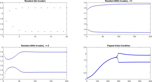
Figure 5. Resident population densities (vertical axes) plotted against years (horizontal axes) for an unstable, more powerful resident (${\alpha }_R=12.672$ and ${\mu }_R=0.7$) and stable, less powerful invader (${\alpha }_I=1.8$ and ${\mu }_I=0.15$). We consider the behaviour of the resident in the absence of an invader (top left), in the presence of an invader with synchronous birth pulses (top right), in the presence of an invader whose birth pulse is maximally offset from the resident's (bottom left), and in the presence of an invader with a slightly offset birth pulse (bottom right).

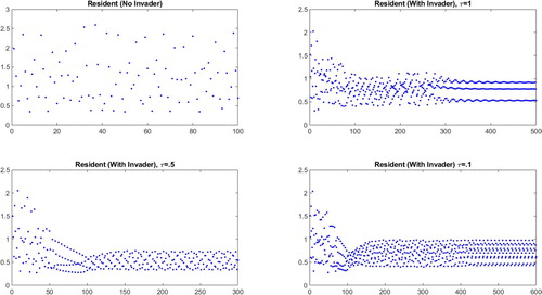
Figure 6. Resident population densities plotted against years (horizontal axes) for an unstable, more powerful resident (${\alpha }_R=8.1$ and ${\mu }_R=0.5$) and stable, less powerful invader (${\alpha }_I=1.8$ and ${\mu }_I=0.15$). We consider the behaviour of the resident in the absence of an invader (top left), in the presence of an invader with synchronous birth pulses (top right), in the presence of an invader whose birth pulse is maximally offset from the resident's (middle left), in the presence of an invader with a moderately offset birth pulse (middle right and bottom left), and when the resident begins from a lower initial condition (bottom right).

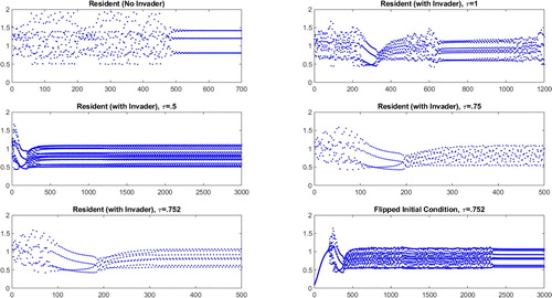
Row 8 is the same as row 4 with the roles of invader and resident reversed, with the only difference being that the stable population now has an equilibrium initial population (instead of a small initial population), and the population with the higher power now has a small initial population (instead of an equilibrium initial population). In these cases, the results are the same as for row 4, except that it takes longer for the system to settle into its cycle (see the final panel of Figure 4).

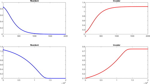
To complete row 6, where the invader and resident are both stable and the invader has higher power, our simulations in Figure 7 show that the resident does not persist. This is consistent with the conjecture that initial conditions do not matter in the long run for this system. It is also consistent with the conjecture that the last four rows of Table 2 have the indicated symmetry with the first four rows.

Figure 7. Resident (left) and invader (right) population densities plotted against years (horizontal axes), for both species stable. In the top panels, the invader is more powerful than the resident (${\alpha }_I=7.66$ and ${\mu }_I=0.8$, ${\alpha }_R=1.35$ and ${\mu }_R=0.2$), with a difference in power scores of 0.004. In the bottom panels, the invader is more powerful than the resident (${\mu }_I=0.05$, ${\alpha }_R=14.6$ and ${\mu }_R=1.6$, $P_I=0.7302$ and $P_R=0.7292$), but the difference in power scores is only 0.001.

The cases in rows 3 and 7 are more complicated than the others because neither consumer species has a stable equilibrium when present as the sole consumer. The best that can be said in these cases is that the competition never results in stable equilibrium (Proposition 1) and that examples suggest that the species with the higher power always persists if it is the resident and invades successfully if it is not. These latter statements must remain conjectural because of the impossibility of obtaining general results. Any attempt to illustrate the possible outcomes with a limited number of figures would be pointless in light of the variety of outcomes and lack of any discernible pattern.

The mathematical and simulation results combine to suggest a hierarchy of rules that determine the outcomes.

1. Stability of the stronger competitor is definitive; that is, the final outcome is that the stronger competitor maintains or reaches its stable equilibrium while the weaker competitor fails to invade (rows 1 and 2) or disappears (rows 5 and 6).

2. Higher power without stability confers sufficient advantage to guarantee the ability to invade (rows 7 and 8) or persist (rows 3 and 4).

3. The combination of instability of the stronger competitor and stability of the weaker competitor evens the fight enough that the weaker competitor might be able to invade (row 4) or persist (row 8).

5. The effect of toxins on competition

We now consider a case study designed to investigate the effect of the timing of a toxic pulse on the competition between two species. We think of the competitors as being two fish species in a lake, a native species 1 that spawns at time s = 1 and an invasive species 2 that spawns at time $s=\tau$ and has a competitive advantage over species 1: (33) $P_1=\frac{{\alpha }_1}{1-{\mathrm{e}}^{{\mu }_1}}<\frac{{\alpha }_2}{1-{\mathrm{e}}^{{\mu }_2}}=P_2.$(33) The toxin is dumped into the lake annually at times $n+{\tau }_0$, $n=0,1,2,\dots$, in such a way that the concentration is periodic, and decays exponentially until the next dumping; that is, (34) $\sigma (s)=\{\begin{array}{ll}m{\mathrm{e}}^{-\mu (1-{\tau }_0)}{\mathrm{e}}^{-\mu s}& s\in [0,{\tau }_0),\\ m{\mathrm{e}}^{-\mu (s-{\tau }_0)}& s\in [{\tau }_0,1],\end{array}$(34) where m is the concentration of the toxin at its annual peak and μ is a rate constant for the decay of the toxin. We assume that the effect of the toxin is to reduce the birth rates $b_j(s)$ by a factor $g(\sigma (s))$, where $g(0)=1$ (no suppression if no toxin) and $g^{\prime }<0$ (diminishing effect of lower toxin levels).

We address the following question: For what values of ${\tau }_0>0$ and $\mu >0$, if any, will the addition of the toxin give the competitive advantage to the native species, that is, lead to species 1 persisting while species 2 goes extinct?

From (33(33) $P_1=\frac{{\alpha }_1}{1-{\mathrm{e}}^{{\mu }_1}}<\frac{{\alpha }_2}{1-{\mathrm{e}}^{{\mu }_2}}=P_2.$(33) ), we see that in the presence of the toxin, the power of species 1 is effectively $g(\sigma (0))P_1$, since for species 1 the toxin acts at the spawning time $0^{-}$ (and g is continuous). Similarly, the power of species 2 is effectively $g(\sigma (\tau ))P_2$, since the toxin acts at the spawning time τ. Thus species 1 has a competitive advantage if and only if (35) $g(\sigma (0))P_1>g(\sigma (\tau ))P_2.$(35) For (35(35) $g(\sigma (0))P_1>g(\sigma (\tau ))P_2.$(35) ) to happen, it is necessary but not sufficient that $g(\sigma (\tau ))<g(\sigma (0))$, or equivalently $\sigma (\tau )>\sigma (0)$. Taking note of (34(34) $\sigma (s)=\{\begin{array}{ll}m{\mathrm{e}}^{-\mu (1-{\tau }_0)}{\mathrm{e}}^{-\mu s}& s\in [0,{\tau }_0),\\ m{\mathrm{e}}^{-\mu (s-{\tau }_0)}& s\in [{\tau }_0,1],\end{array}$(34) ), this means that ${\tau }_0\in [0,\tau ]$, leading to the following proposition (which is clearly true on biological grounds):

Proposition 5.1

The release at times $n+{\tau }_0$ of a toxin that affects the birth rates of two competitors equally can help the weaker resident resist invasion and extinction only if $0<{\tau }_0<\tau$; that is, the pulse of toxin must come in the time interval between each resident birth pulse and the next invader birth pulse.

When Proposition 5.1 is satisfied, the resident benefits more from the toxin when its release is closer to the time of the invader birth pulse (that is; larger ${\tau }_0$ benefits the resident, provided ${\tau }_0<\tau$). As an example, consider the simple toxic effect function $g(\sigma )={\mathrm{e}}^{-k\sigma },$where k is a positive parameter that measures the sensitivity of the birth pulse suppression to the level of toxin.

Some simple computation shows that (35(35) $g(\sigma (0))P_1>g(\sigma (\tau ))P_2.$(35) ) holds if and only if $\mu {\tau }_0>\ln \left[\frac{\ln (P_2/P_1)}{km({\mathrm{e}}^{-\mu \tau }-{\mathrm{e}}^{-\mu })}\right],$where the right-hand side is guaranteed to be positive by (33(33) $P_1=\frac{{\alpha }_1}{1-{\mathrm{e}}^{{\mu }_1}}<\frac{{\alpha }_2}{1-{\mathrm{e}}^{{\mu }_2}}=P_2.$(33) ). Hence, the resident wins the competition if and only if (36) $\frac{1}{\mu }\ln \left[\frac{\ln (P_2/P_1)}{km({\mathrm{e}}^{-\mu \tau }-{\mathrm{e}}^{-\mu })}\right]<{\tau }_0<\tau .$(36) This can always be achieved if ${\tau }_0$ and one of the toxicity parameters μ, m, and k can be freely chosen. If we think of the toxicity parameters as fixed, the timing ${\tau }_0$ can be chosen to give species 1 the competitive advantage if and only if (37) $\ln \left(\frac{P_2}{P_1}\right)<km(1-{\mathrm{e}}^{-\mu (1-\tau )}).$(37)

6. Discussion

We briefly discuss here the main themes of this paper. In our competition model (25(25) $\begin{array}{rl}\frac{\mathrm{d}f}{\mathrm{d}s}& =\rho f(1-f-x-y),f(0)=u_t,u_{t+1}=f(1);\end{array}$(25) )–(30(30) $\begin{array}{rl}{z}_1& =1+b_1(1),z_2=1+b_2({\tau }^{-}).\end{array}$(30) ), the only competition is for resources, with no direct (interference) competition. This implies that the principle of competitive exclusion should hold. Proposition 3.1 gives a limited type of competitive exclusion, where (except on a set of measure zero in the parameter space) there cannot exist a fixed point with mutual survival of both consumers, but where mutual survival without a fixed point is not ruled out. Our main interest is in conditions under which one consumer can successfully invade when the other consumer is at equilibrium. We introduce the concept of the power P of a consumer, which is the average consumer level at equilibrium, while the average resource level is 1−P. Proposition 3.2 can be interpreted as saying that the invader grows when the resource level with which it can coexist at steady-state is less than the steady-state resource level in the resident system. Thus Proposition 3.2 and Corollary 3.1 say, roughly, that the population with the higher power should ‘win '. However, this paradigm can break down when the consumer with the lower power has parameters that satisfy the single consumer stability criteria (16(16) $\frac{1}{M}>1-q,\frac{1}{M}>\frac{1-\delta }{1+\delta }(q-\frac{1}{2}),$(16) ) and its slightly stronger competitor does not. In other words, stability can also give a competitive edge, allowing a slightly weaker consumer to coexist, in violation of the classical principle of competitive exclusion. This is illustrated in Table 2. Negative effects from toxins and differences in birth pulse timing can also change the competition outcome. This should not be considered a violation of competitive exclusion, however, as having different birth pulse timing means that the consumers occupy slightly different ecological niches.

Acknowledgments

We would like to thank Professor Roger Nisbet, of the Department of Ecology, Evolution and Marine Biology at the University of California – Santa Barbara, for helpful suggestions about the formulation of this problem.

Disclosure statement

No potential conflict of interest was reported by the author(s).

Additional information

Funding

This work was supported in part by funding from the Research Experiences for Undergraduate Faculty program, which is partially funded by the National Science Foundation through the Division of Mathematical Sciences Grants 1620073 to the American Institute of Mathematics and 1620080 to Institute for Computational and Experimental Research in Mathematics. This work was also partially supported by Simons Foundation Collaboration Grant 579483.

Appendix 1

Derivation of the fixed points and stability conditions for the single consumer model

Analysis of the single consumer model determines the fixed points $(u^{\ast },v^{\ast })$ and inequalities to determine the stability boundaries in the parameter space. A form of these results was derived in Pachepsky et al., Appendix A. Here, we offer a modification of their analysis for the purpose of obtaining simpler versions of the stability inequalities. The starting point for this analysis is the single consumer model (A1) $\begin{array}{rl}\frac{\mathrm{d}f}{\mathrm{d}s}& =\rho f(1-f-x),f(0)=u_t,u_{t+1}=f(1);\end{array}$(A1) (A2) $\begin{array}{rl}\frac{\mathrm{d}x}{\mathrm{d}s}& =-\mu x,x(0)=v_t,v_{t+1}=x(1^{+})=zx(1^{-});\end{array}$(A2) (A3) $\begin{array}{rl}\frac{\mathrm{d}b}{\mathrm{d}s}& =\alpha f,b(0)=0;\end{array}$(A3) (A4) $\begin{array}{rl}z& =1+b(1^{-});\end{array}$(A4) where we have suppressed the subscript 1 that distinguishes parameters for the two consumer species in the full two-species model.

Before commencing the analysis, we define the parameters (A5) $\overline{f}=\frac{{\mathrm{e}}^{\mu }-1}{\alpha },\overline{x}=1-\overline{f},$(A5) which were shown in the main paper to be the mean values of f and x when the fixed point and associated periodic solution are stable, and the additional combined parameters (A6) $A=\frac{\alpha (1-{\mathrm{e}}^{-\mu })}{\mu }>0,M=(\alpha +1){\mathrm{e}}^{-\mu }-1>0,\delta ={\mathrm{e}}^{-\rho \overline{f}}.$(A6)

A.1. The discrete map

The system A1(A1) $\begin{array}{rl}\frac{\mathrm{d}f}{\mathrm{d}s}& =\rho f(1-f-x),f(0)=u_t,u_{t+1}=f(1);\end{array}$(A1) –A4(A4) $\begin{array}{rl}z& =1+b(1^{-});\end{array}$(A4) defines a discrete map from $(u_t,v_t)$ to $(u_{t+1},v_{t+1})$. We begin by associating a pair of functions g and h with this discrete map in the form (A7) $\begin{array}{c}{u}_{t+1}=u_{t}g(u_t,v_t),\\ v_{t+1}=v_{t}h(u_t,v_t);\end{array}$(A7) this has the advantage that the coexistence fixed point is then determined by the equations g = h = 1.

The analysis requires solution of the continuous problem to determine the functions g and h, calculation of the coexistence fixed point, and determination of the stability criteria from the Jury conditions (see Ledder, Appendix A1, for example).

A.2. An expression for h in terms of g

The function h in the map (A7(A7) $\begin{array}{c}{u}_{t+1}=u_{t}g(u_t,v_t),\\ v_{t+1}=v_{t}h(u_t,v_t);\end{array}$(A7) ) can be found in terms of z from (A2(A2) $\begin{array}{rl}\frac{\mathrm{d}x}{\mathrm{d}s}& =-\mu x,x(0)=v_t,v_{t+1}=x(1^{+})=zx(1^{-});\end{array}$(A2) ): (A8) $h(u_t,v_t)=\frac{v_{t+1}}{v_t}=\frac{zx(1^{-})}{x(0)}={\mathrm{e}}^{-\mu }z.$(A8) To calculate z, we rewrite (A1(A1) $\begin{array}{rl}\frac{\mathrm{d}f}{\mathrm{d}s}& =\rho f(1-f-x),f(0)=u_t,u_{t+1}=f(1);\end{array}$(A1) ) as $\frac{1}{\rho f}\frac{\mathrm{d}f}{\mathrm{d}s}=1-f-x=1-\frac{1}{\alpha }\frac{\mathrm{d}b}{\mathrm{d}s}+\frac{1}{\mu }\frac{\mathrm{d}x}{\mathrm{d}s}$and then integrate from s = 0 to s = 1, yielding $\frac{1}{\rho }\ln \frac{f(1)}{f(0)}=1-\frac{1}{\alpha }b(1^{-})+\frac{1}{\mu }[x(1^{-})-x(0^{+})].$Using $f(1)/f(0)=u_{t+1}/u_t=g(u_t,v_t)$ from (A7(A7) $\begin{array}{c}{u}_{t+1}=u_{t}g(u_t,v_t),\\ v_{t+1}=v_{t}h(u_t,v_t);\end{array}$(A7) ), $b(1^{-})=z-1$ from (A4(A4) $\begin{array}{rl}z& =1+b(1^{-});\end{array}$(A4) ), and $x(0^{+})-x(1^{-})=x(0^{+})-{\mathrm{e}}^{-\mu }x(0^{+})=(1-{\mathrm{e}}^{-\mu })v_t$ from (A8(A8) $h(u_t,v_t)=\frac{v_{t+1}}{v_t}=\frac{zx(1^{-})}{x(0)}={\mathrm{e}}^{-\mu }z.$(A8) ) and (A2(A2) $\begin{array}{rl}\frac{\mathrm{d}x}{\mathrm{d}s}& =-\mu x,x(0)=v_t,v_{t+1}=x(1^{+})=zx(1^{-});\end{array}$(A2) ), we obtain $\frac{1}{\rho }\ln g(u_t,v_t)=1-\frac{1}{\alpha }(z-1)-\frac{1-{\mathrm{e}}^{-\mu }}{\mu }{v}_t,$which rearranges as $z=\alpha +1-A{v}_t-\frac{\alpha }{\rho }\ln g(u_t,v_t).$Combining this last result with (A8(A8) $h(u_t,v_t)=\frac{v_{t+1}}{v_t}=\frac{zx(1^{-})}{x(0)}={\mathrm{e}}^{-\mu }z.$(A8) ) yields an expression for h in terms of g: (A9) $h(u,v)={\mathrm{e}}^{-\mu }[\alpha +1-Av-\frac{\alpha }{\rho }\ln g(u,v)].$(A9)

A.3. An expression for g

Before finding the function $g(u,v)$, it is helpful to define some auxiliary functions by (A10) $R(s;v)=s-\frac{v}{\mu }(1-{\mathrm{e}}^{-\mu s}),G(s;v)={\mathrm{e}}^{\rho R(s;v)},I(v)={\int }_0^{1}G(s;v)\mathrm{d}s.$(A10) The semicolons in the notation for R and G indicate that derivatives will be with respect to s only; for example, (A11) $R^{\prime }=1-v{\mathrm{e}}^{-\mu s}=1-x.$(A11) The values of R and G at s = 1 are particularly important; these are given as (A12) $R_1(v)=R(1;v)=1-\frac{Av}{\alpha },G_1(v)=G(1;v)={\mathrm{e}}^{\rho R_1(v)}.$(A12) With (A11(A11) $R^{\prime }=1-v{\mathrm{e}}^{-\mu s}=1-x.$(A11) ), the problem (A1(A1) $\begin{array}{rl}\frac{\mathrm{d}f}{\mathrm{d}s}& =\rho f(1-f-x),f(0)=u_t,u_{t+1}=f(1);\end{array}$(A1) ) can be written as (A13) $f^{\prime }=\rho f(R^{\prime }-f),f(0)=u,f(1)=ug(u,v).$(A13) To solve this problem, we make the change of variable $\tilde{f}=\frac{1}{f}$, which converts (A13(A13) $f^{\prime }=\rho f(R^{\prime }-f),f(0)=u,f(1)=ug(u,v).$(A13) ) into the linear problem (A14) ${\tilde{f}}^{\prime }+\rho R^{\prime }\tilde{f}=\rho ,\tilde{f}(0)=\frac{1}{u},\tilde{f}(1)=\frac{1}{ug(u,v)}.$(A14) The integrating factor for the differential equation is $G(s;v)$, so we have $(G\tilde{f}{)}^{\prime }=\rho G.$Integrating from s = 0 to s = 1 then yields $\frac{G(1;v)}{ug(u,v)}-\frac{1}{u}=\rho I(v),$from which we obtain the final result (A15) $g(u,v)=\frac{G_1(v)}{1+\rho uI(v)}.$(A15)

A.4. The fixed point

The fixed point satisfies g = h = 1, from which (A9(A9) $h(u,v)={\mathrm{e}}^{-\mu }[\alpha +1-Av-\frac{\alpha }{\rho }\ln g(u,v)].$(A9) ) yields the fixed point component (A16) $v^{\ast }=\frac{\alpha +1-{\mathrm{e}}^{\mu }}{A}=\frac{{\mathrm{e}}^{\mu }M}{A}.$(A16) Some tedious algebra eventually yields (A17) $G^{\ast }(s)\equiv G(s,v^{\ast })=\exp (\rho s-\rho \overline{x}\frac{1-{\mathrm{e}}^{-\mu s}}{1-{\mathrm{e}}^{-\mu }}),G_1(v^{\ast })={\delta }^{-1},$(A17) and then (A18) $I^{\ast }\equiv I(v^{\ast })={\int }_0^1{G}^{\ast }(s)\mathrm{d}s,$(A18) allowing us to identify the fixed point component $u^{\ast }$ as the unique solution of the equation (A19) $1+\rho u^{\ast }{I}^{\ast }={\delta }^{-1}.$(A19)

A.5. The trace and determinant of the Jacobian

The Jacobian for the fixed point $(u^{\ast },v^{\ast })$, given that $g^{\ast }=h^{\ast }=1$, is $J^{\ast }=\left[\begin{array}{cc}1+u^{\ast }{g}_u^{\ast }& u^{\ast }{g}_v^{\ast }\\ v^{\ast }{h}_u^{\ast }& 1+v^{\ast }{h}_v^{\ast }\end{array}\right],$and the corresponding trace and determinant are (A20) $\begin{array}{rl}& T=2+u^{\ast }{g}_u^{\ast }+v^{\ast }{h}_v^{\ast },\end{array}$(A20) (A21) $\begin{array}{rl}& D=1+u^{\ast }{g}_u^{\ast }+v^{\ast }{h}_v^{\ast }+u^{\ast }{v}^{\ast }(g_u^{\ast }{h}_v^{\ast }-h_u^{\ast }{g}_v^{\ast }).\end{array}$(A21) To evaluate these quantities, we first differentiate (A9(A9) $h(u,v)={\mathrm{e}}^{-\mu }[\alpha +1-Av-\frac{\alpha }{\rho }\ln g(u,v)].$(A9) ) and use the equilibrium relation $g^{\ast }=1$ to obtain $h_u^{\ast }=-\frac{\alpha }{\rho }{\mathrm{e}}^{-\mu }{g}_u^{\ast },h_v^{\ast }=-{\mathrm{e}}^{-\mu }A-\frac{\alpha }{\rho }{\mathrm{e}}^{-\mu }{g}_v^{\ast }$or (A22) $v^{\ast }{h}_u^{\ast }=-\frac{\alpha M}{\rho A}{g}_u^{\ast },v^{\ast }{h}_v^{\ast }=-M-\frac{\alpha M}{\rho A}{g}_v^{\ast }.$(A22) From these results, we have $v^{\ast }(g_u^{\ast }{h}_v^{\ast }-h_u^{\ast }{g}_v^{\ast })=-M{g}_u^{\ast }$which simplifies the determinant to (A23) $D=1+(1-M)u^{\ast }{g}_u^{\ast }+v^{\ast }{h}_v^{\ast }.$(A23)

We continue evaluation of the trace and determinant by differentiating (A15(A15) $g(u,v)=\frac{G_1(v)}{1+\rho uI(v)}.$(A15) ) with respect to u, which yields $g_u=\frac{-\rho G_{1}I}{(1+\rho uI{)}^2}.$Evaluating this expression at the fixed point, using (A19(A19) $1+\rho u^{\ast }{I}^{\ast }={\delta }^{-1}.$(A19) ) to eliminate $\rho u^{\ast }I(v^{\ast })$ and $G_1(v^{\ast })$, yields (A24) $u^{\ast }{g}_u^{\ast }=-(1-\delta ).$(A24) Similarly, the more complicated differentiation of (A15(A15) $g(u,v)=\frac{G_1(v)}{1+\rho uI(v)}.$(A15) ) with respect to v yields $g_v=\frac{G_1^{\prime }}{1+\rho uI}-\frac{\rho u{G}_1{I}^{\prime }}{(1+\rho uI{)}^2},$which simplifies at the fixed point to $g_v^{\ast }=-\frac{\rho A}{\alpha }-\rho \delta u^{\ast }{I}^{\prime }(v^{\ast }).$Rewriting (A19(A19) $1+\rho u^{\ast }{I}^{\ast }={\delta }^{-1}.$(A19) ) as $\rho \delta uI=1-\delta$ allows us to write this last result as $g_v^{\ast }=-\frac{\rho A}{\alpha }-(1-\delta )\frac{I^{\prime }(v^{\ast })}{I(v^{\ast })}=-\frac{\rho A}{\alpha }[1+(1-\delta )\frac{\alpha I^{\prime }(v^{\ast })}{\rho AI(v^{\ast })}]$or (A25) $g_v^{\ast }=-\frac{\rho A}{\alpha }[1-(1-\delta )q],$(A25) where (A26) $q=-\frac{\alpha I^{\prime }(v^{\ast })}{\rho AI(v^{\ast })}=\frac{{\int }_0^1(1-{\mathrm{e}}^{-{\mu }_{1}s})G(s,v^{\ast })\mathrm{d}s}{{\int }_0^1(1-{\mathrm{e}}^{-{\mu }_1})G(s,v^{\ast })\mathrm{d}s}.$(A26) Substituting (A25(A25) $g_v^{\ast }=-\frac{\rho A}{\alpha }[1-(1-\delta )q],$(A25) ) into (A22(A22) $v^{\ast }{h}_u^{\ast }=-\frac{\alpha M}{\rho A}{g}_u^{\ast },v^{\ast }{h}_v^{\ast }=-M-\frac{\alpha M}{\rho A}{g}_v^{\ast }.$(A22) ) yields (A27) $v^{\ast }{h}_v^{\ast }=-(1-\delta )Mq,$(A27) after which we may write the trace and determinant as (A28) $T=1+\delta -(1-\delta )qM,D=\delta +(1-\delta )(1-q)M.$(A28)

A.6. Stability by the Jury conditions

Local asymptotic stability requires satisfaction of the Jury necessary conditions (see Ledder, Appendix 1, for example) $D<1,D+1+T>0,D+1-T>0.$The third of these is satisfied automatically, given M>0. The other two are conveniently expressed as upper bounds for M in the form (A29) $\frac{1}{M}>1-q,\frac{1}{M}>\frac{1-\delta }{1+\delta }(q-\frac{1}{2}).$(A29) Replacing ‘>’ with ‘=’ in (A29(A29) $\frac{1}{M}>1-q,\frac{1}{M}>\frac{1-\delta }{1+\delta }(q-\frac{1}{2}).$(A29) ) yields relations that determine the stability boundaries; the first one is the blue curve in Figure 1, while the latter is the red curve.

References

- L. Chen, J. Sun, F. Chen, and L. Zhao, Extinction in a Lotka–Volterra competitive system with impulse and the effect of toxic substances, Appl. Math. Model. 40 (2016), pp. 2015–2024.
- B. Emerick, A. Singh, The effects of host-feeding on stability of discrete-time host-parasitoid population dynamic models, Math. Biosci. 272 (2016), pp. 54–63.
- Z. Jin, H. Maoan, and L. Guihua, The persistence in a Lotka–Volterra competition systems with impulsive, Chaos Soliton Fract 24 (2005), pp. 1105–1117.
- Z. Jin, M. Zhien, and H. Maoan, The existence of periodic solutions of the n-species Lotka–Volterra competition systems with impulsive, Chaos Soliton Frac 22 (2004), pp. 181–188.
- V. Le Bourlot, T. Tully, and D. Claessen, Interference versus exploitative competition in the regulation of size-structured populations, Am. Nat. 184 (2014), pp. 609–623.
- Z. Liu and L. Chen, Periodic solution of a two-species competitive system with toxicant and birth pulse, Chaos Soliton Fract 32 (2007), pp. 1703–1712.
- B. Liu and L. Zhang, Dynamics of a two-species Lotka–Volterra competition system in a polluted environment with pulse toxicant input, Appl. Math. Comput. 214 (2009), pp. 155–162.
- L. Mailleret and V. Lemesle, A note on semi-discrete modelling in the life sciences, Philos. Trans. R. Soc. A: Math. Phys. Eng. Sci. 367 (2009), pp. 4779–4799.
- W.W. Murdoch, C.J. Briggs, R.M. Nisbet, Consumer-Resource Dynamics, Vol. 36, Princeton University Press, Princeton, NJ, 2003.
- T. Nakazawa and H. Doi, A perspective on match/mismatch of phenology in community contexts, Oikos 121 (2012), pp. 489–495.
- L. Nedorezov, About a continuous-discrete model of fish population dynamics, Popul. Dyn.: Anal. Model. Forecast 2 (2011), pp. 129–140.
- E. Pachepsky, R.M. Nisbet, W.W. Murdoch, Between discrete and continuous: Consumer–resource dynamics with synchronized reproduction, Ecology 89 (2008), pp. 280–288.
- T.A. Revilla, F. Encinas-Viso, and M. Loreau, (A bit) earlier or later is always better: Phenological shifts in consumer–resource interactions, Theor. Ecol. 7 (2014), pp. 149–162.
- A. Singh and R.M. Nisbet, Semi-discrete host–parasitoid models, J. Theor. Biol. 247 (2007), pp. 733–742.
- A.T. Tredennick, P.B. Adler, and F.R. Adler, The relationship between species richness and ecosystem variability is shaped by the mechanism of coexistence, Ecol. Lett. 20 (2017), pp. 958–968.