Complexity of host-vector dynamics in a two-strain dengue model

Abstract

We introduce a compartmental host-vector model for dengue with two viral strains, temporary cross-immunity for the hosts, and possible secondary infections. We study the conditions on existence of endemic equilibria where one strain displaces the other or the two virus strains co-exist. Since the host and vector epidemiology follow different time scales, the model is described as a slow-fast system. We use the geometric singular perturbation technique to reduce the model dimension. We compare the behaviour of the full model with that of the model with a quasi-steady approximation for the vector dynamics. We also perform numerical bifurcation analysis with parameter values from the literature and compare the bifurcation structure to that of previous two-strain host-only models.

Keywords:

• Vector-borne disease dynamics
• Dengue
• two-strain model
• bifurcation analysis

2010 Mathematics Subject Classifications:

• 35B32
• 37N25
• 92D30

1. Introduction

Dengue fever is a tropical disease caused by an arbovirus and spread by female mosquitos of the genus Aedes. Its epidemiology is characterized by the possibility of multiple reinfections of an individual due to the presence of four viral strains which co-circulate in the tropical regions of the Earth [34]. Individuals who have experienced a primary infection with one dengue strain develop life-long immunity against this strain, but after a period of temporary cross-immunity against the other strains become again susceptible to a different dengue strain. Secondary infections may result in health complications such as dengue haemorrhagic fever and pose a health concern in dengue-endemic countries. Mathematical study of dengue epidemiology is motivated by its increasing global incidence in the past decades and recent explosive outbreaks [35].

Epidemiological models often have to find a balance between accurate description of the disease dynamics, the different scales of modelling (within-host/micro scale or population/macro scale), and the associated levels of complexity. By using different dimension reduction arguments to construct mathematically tractable models, it is possible to focus on different aspects of the disease dynamics. While some host-only models include vector dynamics implicitly in the model parameters [1,2,4,18,22,28], etc., studies of effects such as pest control or personal protection via repellents, which influence the mosquito dynamics, speak in favour of an explicit inclusion into the model. In this way, control measures could be tailored to the vector's ecology to achieve an optimum effect as they alter diverse vector characteristics, parametrized in the model as birth and death rates, biting rate, infection rate, etc.

Models of multi-strain dengue epidemiology are based on a susceptible-infected-recovered (SIR) model for the host with the following modification: after recovery from a primary infection with one of the strains, the human hosts gain temporary cross-immunity against both strains, but afterwards become susceptible to possible secondary infection with the other strain. Only after recovery from the secondary infection does a host obtain immunity. Dengue models with two strains and their variations are proposed and studied in [1,2,4,22,23]. These compartmental models are host-only of SIR type. The infected classes distinguish between the viral strains in both primary and secondary infections but do not incorporate explicitly the vector dynamics of mosquitos.

Female mosquitoes, however, play a role in the transmission of the disease and are principal target for most control strategies. Dengue models which include mosquito dynamics explicitly [5,14,15,31,36] add compartments for susceptible and dengue-infected mosquitos. The vector population is governed by a susceptible-infected model because the mosquitos do not recover from the virus. Control strategies for models of single-strain dengue with seasonality have been studied in [5,31] and for a two-strain model without seasonality in [36].

In this study, we consider a variation and extension of these models by introducing susceptible and infected vector classes into host-only models which include susceptible hosts with a background of dengue infection as in [1,2,22,23]. Further, we introduce into the model a parameter that quantifies the differences in likelihood for host-to-vector transmission between infected individuals in a primary and a secondary dengue infection, unlike [36]. Such a parameter serves as a measure whether hosts with a secondary infection have on average a lower or a higher contribution to the overall force of infection upon mosquitos than hosts with a primary infection. This requires besides the new equations also a reinterpretation of the model parameters from [1,4,22,23] which must reflect the per-vector rather than per-host contribution to force of infection. In this way, we incorporate micro-scale factors (immune response) besides macro-scale factors (climate effect on the vector). This allows us to examine parameter regimes corresponding to different scenarios (Section 5). Our model is able to capture phenomena such as seasonal variation and irregular patterns in the incidence of the dengue observed in regions such as Thailand, as well as the co-circulation of dengue strains.

We analyse properties of the full model and study its dynamics in relation to the simplified host-only models, as well as to reduced versions based on quasi-steady state assumptions and geometric singular perturbation analysis as done previously [27]. We also compare the qualitative behaviour of our model that explicitly includes a vector population to those host-only models by performing numerical bifurcation analysis with parameter values from the literature [1,2,22,23]. We also study the bifurcation structure of the autonomous model to a non-autonomous model where seasonal variation in the vector population exists. Our analysis leads us to the conclusion that in order to remain in agreement with seasonally varying data on dengue fever incidence, to reflect disease characteristics of primary vs. secondary infections, and to understand the epidemic complexity, it is essential to include vector ecology in the model. In this way, long-term control strategies for a multi-strain vector-borne disease such as dengue fever could become realistically tractable based on such models.

2. Mathematical model

The host population is subdivided into classes with the following transitions (Figure 1, left): susceptible individuals without a previous dengue infection $S_0$, primary infected with ith strain $I_i$, and recovered $R_i$ from a primary infection respectively with strain $i=1,2$. After a period of a temporary cross-immunity, recovered individuals in class $R_i$ transition to the class $S_i$ of susceptible individuals with a history of a primary dengue infection with ith strain i = 1, 2. These individuals can become infected again with the other virus strain: hosts from $S_1$ transition to class $I_{12}$ and from $S_2$ to class $I_{21}$. Finally individuals from the secondary infected classes $I_{12},I_{21}$ recover and obtain life-long immunity against both strains (class R).

Figure 1. Flow chart of the transitions between the host and vector compartments. The birth and death of hosts and vectors are not explicitly shown for the sake of clarity.

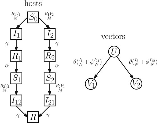
To model the vector dynamics, we follow [15] in assuming that once a mosquito is infected, it never recovers and cannot be reinfected with a different strain because of its short lifespan. We label the susceptible vector population by U and the vector populations carrying i-th dengue strain by $V_i$ (i = 1, 2). Reinfections with the dengue virus of a different strain, therefore, may take place only in the host. We also assume that upon biting an infected individual, a mosquito is infected with the strain that infected individual currently carries (Figure 1, right).

Hence, transmission of the first dengue strain occurs between vector class $V_1$ to host classes $S_0,S_2$ and between host class $I_1,I_{21}$ to vector class U. Similarly, that transmission of the second strain occurs between vectors in class $V_2$ to host classes $S_0,S_1$ and between hosts in classes $I_2,I_{12}$ to vectors in class U.

The cumulative disease transmission parameter $B_j$ (j is the number of consecutive infection a human experiences) is defined as the product of the biting rate r and the per-bite infection probability $p_{vh,j}$ from mosquito vector to human host: $B_j=r{p}_{vh,j},j=1,2$. We assume that $p_{vh,2}\ge p_{vh,1}$, in other words, the infection probability in a secondary dengue infection is equal to or greater than that in a primary infection due to the phenomenon of antibody-dependent enhancement (ADE) [20] leading to $B_2\ge B_1$. Thus, in contrast to [23] the index j of B in our model does not refer to the infectivity of a specific dengue viral strain. As we do not model such strain-specific infectivity, we assume that both strains have equal infectivity upon a susceptible host regardless of his infection background.

The cumulative disease transmission parameter ϑ is the product of the biting rate r with the per-bite infection probability $p_{hv}$ from human host to mosquito vector: $\vartheta =r{p}_{hv}$.

The shape of the force of infection term for mosquitos upon humans and humans upon mosquitos follows [11]. As in [1] individuals recover from any dengue infection after a period of length $1/\gamma$ years and their temporary cross-immunity lasts on average $1/\alpha$ years. The hosts' population demography (human birth and death rates) is parametrized by μ. For the mosquito vector, the demography (mosquito birth and death rates) is parametrized by ν. We assume $\nu \gg \mu$ to account for the significantly longer life span of the human hosts.

It is important for such a model to capture some characteristics of the host-to-vector transmission as well. The factors behind a successful transmission of dengue from an infected human to a biting mosquito are poorly understood [26]. No studies have investigated human host-seeking ability in dengue-infected mosquitos [6]. However, factors such as personal protection measures like use of repellents, protective clothing by asymptomatic patients, or effective isolation of infected patients from mosquitos could influence the dynamics of the disease transmission.

Hence, we exploit this opportunity to study mathematically these characteristics. Unlike Zheng and Nie [36] who assume that individuals with primary and secondary infection have equal contribution to the force of infection upon susceptible mosquitos, we introduce a parameter ϕ that quantifies the difference in transmission likelihood from hosts with primary or secondary infections to vectors.

When ϕ is larger/smaller than 1, individuals in their secondary infection are more/less likely to transmit the disease to mosquitos than individuals in their first infection. This could be due to factors such as changes in biting rates or virus transmission probabilities. This differs from the interpretation of the parameter ϕ in models such as [1,4,22] where ϕ quantifies the effect of ADE, but rather relates to its interpretation as disease transmissibility during a secondary infection as defined by [28]. We note the models in [1,4,22,28] do not include explicitly any vector population.

A value $\varphi <1$ corresponds to a scenario where hosts with a secondary infection have on average a lower contribution to the overall infectivity of mosquitos upon humans than hosts with a primary infection. A reason behind this could be that secondary infection is clinically more apparent (due to disease severity) and thus more people seek medical care and need hospitalization [7]. Hence, such individuals have on average a lower chance of exposure to mosquitos on search for a blood meal, and the cumulative rate ϑ is then lowered by a factor of ϕ.

A value $\varphi >1$ corresponds to a scenario where hosts with a secondary infection have on average a higher contribution to the overall infectivity of mosquitos upon humans than hosts with a primary infection. In particular, the transmission likelihood from host to vector could be greater if during the course of a secondary infection, the infected host is more attractive to mosquitos on search for a blood meal, because, e.g. of physiological symptoms such as high tympanic temperature or higher viral titres in the host's blood [26]. In particular, evidence suggests a higher mean maximum body temperature in patients is usually associated with a secondary infection [7].

2.1. Model equations

Initially we assume both the host population size N and the vector population size M are constant in time. Hence, the dimension of system can be reduced by eliminating two of the variables by setting $U=M-V_1-V_2$ and $R=N-S_0-S_1-S_2-I_1-I_2-I_{12}-I_{21}-R_1-R_2$. We shall work with the following autonomous system of ordinary differential equations: (1a) $\begin{array}{rl}\frac{\mathrm{d}}{\mathrm{d}t}{S}_0& =-\frac{B_1}{M}{S}_0(V_1+V_2)+\mu (N-S_0)\end{array}$(1a) (1b) $\begin{array}{rl}\frac{\mathrm{d}}{\mathrm{d}t}{I}_1& =\frac{B_1}{M}{S}_0{V}_1-(\gamma +\mu )I_1\end{array}$(1b) (1c) $\begin{array}{rl}\frac{\mathrm{d}}{\mathrm{d}t}{I}_2& =\frac{B_1}{M}{S}_0{V}_2-(\gamma +\mu )I_2\end{array}$(1c) (1d) $\begin{array}{rl}\frac{\mathrm{d}}{\mathrm{d}t}{R}_1& =\gamma I_1-(\alpha +\mu )R_1\end{array}$(1d) (1e) $\begin{array}{rl}\frac{\mathrm{d}}{\mathrm{d}t}{R}_2& =\gamma I_2-(\alpha +\mu )R_2\end{array}$(1e) (1f) $\begin{array}{rl}\frac{\mathrm{d}}{\mathrm{d}t}{S}_1& =\alpha R_1-\mu S_1-\frac{B_2}{M}{S}_1{V}_2\end{array}$(1f) (1g) $\begin{array}{rl}\frac{\mathrm{d}}{\mathrm{d}t}{S}_2& =\alpha R_2-\mu S_2-\frac{B_2}{M}{S}_2{V}_1\end{array}$(1g) (1h) $\begin{array}{rl}\frac{\mathrm{d}}{\mathrm{d}t}{I}_{12}& =\frac{B_2}{M}{S}_1{V}_2-(\gamma +\mu )I_{12}\end{array}$(1h) (1i) $\begin{array}{rl}\frac{\mathrm{d}}{\mathrm{d}t}{I}_{21}& =\frac{B_2}{M}{S}_2{V}_1-(\gamma +\mu )I_{21}\end{array}$(1i) (1j) $\begin{array}{rl}\frac{\mathrm{d}}{\mathrm{d}t}{V}_1& =\frac{\vartheta }{N}(M-V_1-V_2)(I_1+\varphi I_{21})-\nu V_1\end{array}$(1j) (1k) $\begin{array}{rl}\frac{\mathrm{d}}{\mathrm{d}t}{V}_2& =\frac{\vartheta }{N}(M-V_1-V_2)(I_2+\varphi I_{12})-\nu V_2\end{array}$(1k) where $\frac{\mathrm{d}}{\mathrm{d}t}$ denotes the time derivative.

Observe that for the host infection rate the symbol B is used instead of β to avoid a misinterpretation. In host-only models [2,4,18,22] infection rate per infected host β was used and in host-vector models [27,29] as well as here infection rate per infected vector.

Implicitly in [2,22] and other earlier models described in [4,18], the vector dynamics was taken into account by assuming that the size of the infected vector population is proportional to that of the infected human-host population. The two-strain host-only model is described in the Appendix (A1).

In [27], the following equation was derived for the relationship of the infection rates in the host-vector model $B_i$ and the host-only model ${\beta }_i$: (2) $\frac{B_i}{M}V=\frac{B_i}{M}\frac{\vartheta M}{\nu N}I=\frac{{\beta }_i}{N}I\mathrm{with}{\beta }_i=\frac{\vartheta }{\nu }{B}_i.$(2) Using the values from [1,22] this yields $B_i={\beta }_i/2$, and makes it possible to compare the results of the host-vector model (1) with those from for the host-only model (A1) in [22].

The biologically relevant domain for (1) is $\begin{array}{rl}\mathrm{\Omega }& =\{(S_0,I_1,I_2,I_{12},I_{21},S_1,S_2,R_1,R_2,V_1,V_2)|0\le V_1+V_2\le M,\\ 0& \le S_0+I_1+R_1+S_1+I_{12}+I_2+R_2+S_2+I_{12}\le N\}.\end{array}$Following [24, Lemma 2.1], one can demonstrate that Ω is positively invariant under (1). The details are not shown here.

We also consider some ecological facts about the mosquito vector, namely, the case of a seasonally changing mosquito population due to climate factors such as temperature or rainfall. The number of mosquito vectors M is modelled as seasonal forcing and is given explicitly by a cosine function (3) $M=M(t)=M_0(1+\eta \cos \omega (t+\phi )).$(3) In (3(3) $M=M(t)=M_0(1+\eta \cos \omega (t+\phi )).$(3) ), $M_0$ is the mean population, η describes the magnitude of the seasonal fluctuation and φ is the phase, which we assume to be zero. The frequency $\omega =1$ models yearly variations in the mosquito population. In this case, the system of governing ordinary differential Equations (1) with (3(3) $M=M(t)=M_0(1+\eta \cos \omega (t+\phi )).$(3) ) becomes non-autonomous.

2.2. Basic reproduction number

In the epidemiological literature, the basic reproduction number denoted by ${\mathcal{R}}_0$ represents the number of secondary cases; one infected case generates on average over the course of its infectious period, in a fully susceptible population [9,10]. There are several approaches to compute ${\mathcal{R}}_0$. We compute the parameter values at which an endemic equilibrium appears (e.g. through a transcritical bifurcation TC, see Table 2), that is, the disease can persist in the population and associate it with the value ${\mathcal{R}}_0=1$.

3. Equilibria and local stability analysis

We perform analysis of the equilibria of the model (1). For sake of shortness, whenever necessary, we denote by $\mathbf{x}(t)=(S_0(t),I_1(t),I_2(t),I_{12}(t),I_{21}(t),S_1(t),S_2(t),R_1(t),R_2(t),V_1(t),V_2(t)).$Of interest for the dynamics of the disease is first, the disease-free equilibrium, where all individuals and mosquitos are susceptible, $S_0=N,U=M$ and all other classes are zero, and second, any endemic equilibria, where some classes of infected individuals and mosquitos are non-zero.

For the sake of clarity in the rest of the paper, we shall denote $\overline{\alpha }\equiv \alpha +\mu ,\overline{\gamma }\equiv \gamma +\mu$.

3.1. Symmetry

The system (1) possesses ${\mathbb{Z}}^2$-symmetry, namely, if we denote the symmetry transformation matrix by $\mathbf{S}=\left[\begin{array}{ccccccccccc}1& 0& 0& 0& 0& 0& 0& 0& 0& 0& 0\\ 0& 0& 1& 0& 0& 0& 0& 0& 0& 0& 0\\ 0& 1& 0& 0& 0& 0& 0& 0& 0& 0& 0\\ 0& 0& 0& 0& 1& 0& 0& 0& 0& 0& 0\\ 0& 0& 0& 1& 0& 0& 0& 0& 0& 0& 0\\ 0& 0& 0& 0& 0& 0& 1& 0& 0& 0& 0\\ 0& 0& 0& 0& 0& 1& 0& 0& 0& 0& 0\\ 0& 0& 0& 0& 0& 0& 0& 0& 1& 0& 0\\ 0& 0& 0& 0& 0& 0& 0& 1& 0& 0& 0\\ 0& 0& 0& 0& 0& 0& 0& 0& 0& 0& 1\\ 0& 0& 0& 0& 0& 0& 0& 0& 0& 1& 0\end{array}\right]$and by F the vector of the right-hand side of (1), we have $F(\mathbf{S}\mathbf{x})=\mathbf{S}F(\mathbf{x}).$We recall that an equilibrium/limit cycle $\overline{\mathbf{x}}$ is called fixed when $\mathbf{S}\overline{\mathbf{x}}=\overline{\mathbf{x}}$. Then the state variables in their own classes are equal, for instance, $I_1(t)=I_2(t)$ for all t. If the solution is a fixed limit cycle, then the variables $S_i,I_i,I_{ij},R_i$ with i, j = 1, 2 are in phase.

Two equilibria/limit cycles ${\overline{\mathbf{x}}}_1,{\overline{\mathbf{x}}}_2$ where $\mathbf{S}{\overline{\mathbf{x}}}_i\ne {\overline{\mathbf{x}}}_i$, are called S-conjugate if their corresponding solutions satisfy ${\overline{\mathbf{x}}}_2=\mathbf{S}{\overline{\mathbf{x}}}_1$ (and because ${\mathbf{S}}^2=\mathbf{I}\mathbf{d}$ also ${\overline{\mathbf{x}}}_1=\mathbf{S}{\overline{\mathbf{x}}}_2$). There is another type of periodic solution with period T that is not fixed but called symmetric when $\mathbf{S}\overline{\mathbf{x}}(t)=\overline{\mathbf{x}}(t+\frac{T}{2}).$In this case, it holds that $I_1(t)=I_2(t+\frac{T}{2}),I_2(t)=I_1(t+\frac{T}{2})$ etc. (see Figure 6). For a detailed discussion of the ${\mathbb{Z}}^2$-symmetry in dengue epidemiology, the reader is referred to [22].

3.2. Disease-free equilibrium

The trivial, disease-free equilibrium of (1) is ${\mathcal{E}}_0=(N,0,0,0,0,0,0,0,0,0,0)$.

Proposition 3.1

Let (4) ${\mathcal{R}}_0=\frac{B_1\vartheta }{\nu \overline{\gamma }}.$(4) The disease-free equilibrium equilibrium ${\mathcal{E}}_0$ is locally asymptotically stable if ${\mathcal{R}}_0\le 1$, and locally asymptotically unstable if ${\mathcal{R}}_0>1$.

The proof is given in the Appendix.

At ${\mathcal{R}}_0=1$, the local stability of the disease-free equilibrium ${\mathcal{E}}_0$ changes. Because two virus strains are present in the epidemiological setting, several endemic equilibria with one or both strains present are possible. We consider first the boundary equilibria in Ω with a single strain. From an ecological viewpoint, this is the case of competitive exclusion of one of the strains.

3.3. One-strain, competitive exclusion equilibria

Let ${\mathcal{E}}_1$ denote the equilibrium where the first dengue strain is absent, so ${\mathcal{E}}_1=(S_{01}^{\ast },0,I_2^{\ast },0,0,0,S_2^{\ast },0,R_2^{\ast },0,V_2^{\ast })$with $S_{01}^{\ast },I_2^{\ast },R_2^{\ast },S_2^{\ast },V_2^{\ast }\ne 0$, and let ${\mathcal{E}}_2$ denote the equilibrium where the second dengue strain is absent, so ${\mathcal{E}}_2=(S_{02}^{\ast },I_1^{\ast },0,0,0,S_1^{\ast },0,R_1^{\ast },0,V_1^{\ast },0)$with $S_{02}^{\ast },I_1^{\ast },R_1^{\ast },S_1^{\ast },V_1^{\ast }\ne 0$. It is straightforward to show using [27] the following

Lemma 3.2

The hyperplanes ${\mathcal{H}}_1=\{\mathbf{x}\in {\mathbb{R}}^{11}|{\mathbf{x}}_j=0,j=2,4,5,6,8,10\}$ and ${\mathcal{H}}_2=\{\mathbf{x}\in {\mathbb{R}}^{11}|{\mathbf{x}}_j=0,j=3,4,5,7,9,11\}$ are positively invariant sets for (1). Furthermore, any trajectory starting in ${\mathcal{H}}_i$ converges to ${\mathcal{E}}_i$ whenever μ is sufficiently small.

Because the model is symmetric in the two strains, the stability analysis of ${\mathcal{E}}_1,{\mathcal{E}}_2$ is analogous, and we shall analyse the linear stability of ${\mathcal{E}}_1$.

In ${\mathcal{E}}_1$, the equilibrium values of the nonzero classes (see Appendix for the derivation) are (5a) $\begin{array}{rl}{S}_{01}^{\ast }& =\frac{N}{B_1+\mu }(\mu +\frac{\nu \overline{\gamma }}{\vartheta }),\end{array}$(5a) (5b) $\begin{array}{rl}{V}_2^{\ast }& =\frac{M\mu }{\mu +\frac{\nu \overline{\gamma }}{\vartheta }}(1-\frac{1}{{\mathcal{R}}_0}),\end{array}$(5b) (5c) $\begin{array}{rl}{I}_2^{\ast }& =\frac{B_{1}N}{\overline{\gamma }}\frac{\mu }{B_1+\mu }(1-\frac{1}{{\mathcal{R}}_0}),\end{array}$(5c) (5d) $\begin{array}{rl}{R}_2^{\ast }& =\frac{\gamma }{\overline{\alpha }}\frac{B_{1}N}{\overline{\gamma }}\frac{\mu }{B_1+\mu }(1-\frac{1}{{\mathcal{R}}_0}),\end{array}$(5d) (5e) $\begin{array}{rl}{S}_2^{\ast }& =\frac{\alpha \gamma }{\overline{\alpha }}\frac{B_{1}N}{\overline{\gamma }}\frac{1}{B_1+\mu }(1-\frac{1}{{\mathcal{R}}_0}).\end{array}$(5e) These values are positive (and they belong to the biologically relevant set Ω) if and only if ${\mathcal{R}}_0>1$. Summarizing the above, we have

Proposition 3.3

The equilibria ${\mathcal{E}}_1,{\mathcal{E}}_2$ exist in Ω when ${\mathcal{R}}_0>1$.

Next we show that under a mild assumption, both competitive exclusion equilibria ${\mathcal{E}}_1,{\mathcal{E}}_2$, are locally asymptotically unstable for all ${\mathcal{R}}_0>1$. This is due to the presence of temporary cross-immunity for the recovered individuals in $R_1,R_2$ modelled by the parameter α. Remember that the average duration of the temporary immunity for these individuals equals $1/\alpha$ years, e.g. $\alpha =2$ corresponds to a duration of 6 months.

Proposition 3.4

The one-strain competitive exclusion equilibria ${\mathcal{E}}_1,{\mathcal{E}}_2$ of (1) are locally asymptotically unstable for all ${\mathcal{R}}_0>1$ if $B_1>\frac{B_2\overline{\gamma }\nu }{\overline{\gamma }\nu +\vartheta (B_2+\mu )}.$

Proof.

Consider exclusion equilibrium ${\mathcal{E}}_1$. For $V_1=0,V_2\ne 0$, we have $I_1=I_{21}=I_{12}=0,R_1=S_1=0$. Denote the Jacobian matrix evaluated at the equilibrium point by ${\mathcal{E}}_1$ by $J_1$ (see Appendix).

The product of the eigenvalues of $J_1$ is the same as $det{J}_1$. Because $J_1$ is an odd-sized matrix, if $det{J}_1>0$, it must have a positive real eigenvalue. We compute $det{J}_1=\frac{\alpha \overline{\alpha }{B}_2\gamma {\mu }^3\nu \varphi {\overline{\gamma }}^2(\overline{\gamma }\nu -B_1\vartheta {)}^2((B_1-B_2)\overline{\gamma }\nu +B_1\vartheta (B_2+\mu ))}{B_1^2(\overline{\gamma }\nu +\mu \vartheta {)}^2}.$Positivity of $\alpha ,\varphi ,\gamma ,\mu ,\nu$ together with the condition $(B_1-B_2)\overline{\gamma }\nu +B_1\vartheta (B_2+\mu )>0$implies $det{J}_1>0$. Therefore, if the condition of Proposition 3.4 is met, the matrix $J_1$ has a positive real eigenvalue.

The analysis of the determinant is analogous for the equilibrium ${\mathcal{E}}_2$.

Thus, both boundary equilibria (in ecological sense, equilibria of competitive exclusion of one dengue virus strain) are S-conjugate and are always saddle points if the susceptibility to a secondary infection is equal to the susceptibility to a primary infection.

Corollary 3.5

Whenever $B_1=B_2$, the condition from Proposition 3.4 holds automatically, so both boundary equilibria are saddle points.

The stable manifold to each ${\mathcal{E}}_i$ is given by the hyperplane ${\mathcal{H}}_i$ listed in Lemma 3.2.

Note, however, if the condition from Proposition 3.4 is not met, we cannot conclude the opposite, namely, that the equilibrium is locally asymptotically stable, without a numerical validation.

To sum up, unlike [15], the model (1) allows for both boundary equilibria to be locally asymptotically unstable. The model in [4] arrives to the same conclusion as Corollary 3.5, namely, due to the equal epidemiological parameters for the dengue strains neither boundary equilibrium will ever be stable.

3.4. Interior, two-strain equilibrium

Next, we consider equilibria where both virus strains are present in the population. In these endemic equilibria, the classes of host individuals and mosquito vectors carrying either strain are strictly positive.

Proposition 3.6

Let $\varphi >0$. The interior endemic equilibrium is given by $\begin{array}{rl}{S}_0& =\frac{\mu N}{\mu +2x},\\ I_1& =I_2=\frac{\mu Nx}{\overline{\gamma }(\mu +2x)},\\ R_1& =R_2=\frac{\gamma }{\overline{\alpha }}{I}_1,\\ S_1& =S_2=\frac{\alpha \gamma \mu N{x}_2}{\overline{\alpha }\overline{\gamma }(\mu +qx)(\mu +2x)},\\ I_{12}& =I_{21}=\frac{\alpha \gamma \mu Nq{x}^2}{\overline{\alpha }{\overline{\gamma }}^2(\mu +qx)(\mu +2x)}.\end{array}$where x is the root of (6) $c_2{x}^2+c_{1}x+c_0=0$(6) with coefficients given by $\begin{array}{rl}{c}_2& =-2\frac{B_2}{B_1}(\varphi \alpha \gamma +\overline{\gamma }\overline{\alpha }+\frac{\nu }{\vartheta \mu }{\overline{\gamma }}^2\overline{\alpha }),\\ c_1& =\overline{\alpha }{B}_2\overline{\gamma }+\alpha B_2\gamma \varphi -2\overline{\alpha }\overline{\gamma }\mu -(2+\frac{B_2}{B_1})\frac{\nu }{\vartheta }{\overline{\gamma }}^2\overline{\alpha },\\ c_0& =\mu \overline{\gamma }\overline{\alpha }(B_1-\frac{\nu }{\vartheta }\overline{\gamma }).\end{array}$This equilibrium is unique if ${\mathcal{R}}_0>1$. There are two interior endemic equilibria if ${\mathcal{R}}_0<1$ and $c_1>0,c_1^2-4c_0{c}_2>0$.

Note that due to the size of the Jacobian we are not able to make conclusions about stability of this equilibrium without resorting to numerical approximation.

When the class of secondary infected individuals is not able to transmit the virus to mosquitos ($\varphi =0$), the interior equilibrium is a curve:

Proposition 3.7

Let $\varphi =0$. The set of interior equilibria ${\mathcal{E}}^{\circ }$ is a curve consisting of the points $\begin{array}{rl}& (\frac{N(\mu +\frac{B_1}{{\mathcal{R}}_0})}{\mu +B_1},\frac{N(B_1+\mu {\mathcal{R}}_0)x_1}{\overline{\gamma }(\mu +B_1){\mathcal{R}}_0},\frac{N(B_1+\mu {\mathcal{R}}_0)x_2}{\overline{\gamma }(\mu +B_1){\mathcal{R}}_0},\frac{\alpha \gamma Nq(B_1+\mu {\mathcal{R}}_0)x_1{x}_2}{\overline{\alpha }{\overline{\gamma }}^2(\mu +q{x}_2)(\mu +B_1){\mathcal{R}}_0},\\ & \frac{\alpha \gamma Nq(B_1+\mu {\mathcal{R}}_0)x_1{x}_2}{\overline{\alpha }{\overline{\gamma }}^2(\mu +q{x}_1)(\mu +B_1){\mathcal{R}}_0},\frac{\alpha \gamma N(B_1+\mu {\mathcal{R}}_0)x_1}{\overline{\alpha }\overline{\gamma }(\mu +q{x}_2)(\mu +B_1){\mathcal{R}}_0},\\ & \frac{\alpha \gamma N(B_1+\mu {\mathcal{R}}_0)x_2}{\overline{\alpha }\overline{\gamma }(\mu +q{x}_1)(\mu +B_1){\mathcal{R}}_0},\frac{N\gamma (B_1+\mu {\mathcal{R}}_0)x_1}{\overline{\alpha }\overline{\gamma }(\mu +B_1){\mathcal{R}}_0},\frac{N\gamma (B_1+\mu {\mathcal{R}}_0)x_2}{\overline{\alpha }\overline{\gamma }(\mu +B_1){\mathcal{R}}_0},\frac{M{x}_1}{B_1},\frac{M{x}_2}{B_1})\end{array}$parametrized by $\{x_1,x_2>0|x_1+x_2=\frac{\mu B_1({\mathcal{R}}_0-1)}{B_1+\mu {\mathcal{R}}_0}\}$. Further, ${\mathcal{E}}^{\circ }$ is a locally stable.

An illustrative example of the parameter ranges for existence of single or pair of interior equilibria is provided in Figure 2.

Figure 2. The range $(B_1,B_2)$ corresponding to 0, 1 or 2 coexistence equilibria (the dashed vertical line is the set with $B_1$ such that ${\mathcal{R}}_0=1$. The shaded area shows the pairs $(B_1,B_2)$ with a locally asymptotically stable interior equilibrium (eigenvalues computed numerically). The parameter values are given in Table 1 and $\varphi =0.5$.

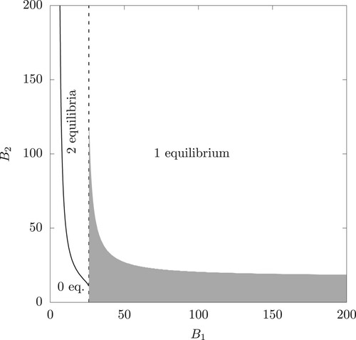
Table 1. Parameter values, most after [1,22] for the host-only model (A1) and [29] for the host-vector model.

Par.	Description
Host
N	Host population density	1000
$B_i$	Infection rate per infected vector	as indicated
${\beta }_i$	Infection rate per infected host	$[0,104]$ (or free)
μ	Susceptible birth rate	1/65
γ	Recovery rate	365/7
α	temporary cross-immunity rate	2, 52 or $[1,250]$
Vector
M	Vector population density	10000
ν	Susceptible birth rate	36.5
ϑ	Infection rate per host	73
η	Magnitude of sinusoidal fluctuation vectors	0 or 0.35
ϕ	Ratio of likelihoods of transmission from hosts with secondary and hosts with primary infection to vectors	$[0,12]$
φ	Phase	0

Notes: The units and values of the infection rate B in this study are different from those in the other references where it is β. Remark: in previous papers N was taken 100 but here 1000. This means that in the comparison the results for the compartments in the previous papers have to be corrected by multiplication with 10.

Details on the proofs of Propositions 3.6 and 3.7 are provided in the Appendix.

3.5. Special case $B_1=B_2$

Whenever the per-bite infection probability from mosquito vector to human host in the secondary infection equals that in the first infection, $p_{vh,1}=p_{vh,2}$, we have $B_1=B_2\equiv B$, and we can simplify the conditions on signs from Proposition 3.6. Denote ${\varrho }_1=\overline{\gamma }\frac{\nu }{\vartheta },{\varrho }_2=\frac{2\vartheta \mu \overline{\gamma }\overline{\alpha }+3\nu {\overline{\gamma }}^2\overline{\alpha }}{\vartheta (\overline{\gamma }\overline{\alpha }+\varphi \alpha \gamma )}.$Whenever $0<B<{\varrho }_2$, $c_1<0$, and otherwise, $c_1>0$ if $B>{\varrho }_2$. Since $\mu \approx 0$ is a small parameter, observe that ${\varrho }_2\approx \frac{2\vartheta \mu +3\nu \gamma }{\vartheta (1+\varphi )}.$Hence, if additionally the discriminant of (6(6) $c_2{x}^2+c_{1}x+c_0=0$(6) ) $\begin{array}{rl}\mathrm{\Delta }& =(\overline{\alpha }\overline{\gamma }+\alpha \gamma \varphi {)}^2{B}^2+2\overline{\alpha }\overline{\gamma }(4(\overline{\alpha }\overline{\gamma }(\mu +{\varrho }_1)+\alpha \gamma \mu \varphi )-(2\mu +3{\varrho }_1)(\overline{\alpha }\overline{\gamma }+\alpha \gamma \varphi ))B\\ & +(2\overline{\alpha }\overline{\gamma }\mu +3\overline{\alpha }\overline{\gamma }{\varrho }_1{)}^2-8\overline{\alpha }\overline{\gamma }{\varrho }_1(\overline{\alpha }\overline{\gamma }(\mu +{\varrho }_1)+\alpha \gamma \mu \varphi )\end{array}$is positive, the quadratic has two positive roots.

Hence, the number of positive solutions of (6(6) $c_2{x}^2+c_{1}x+c_0=0$(6) ) for $B_1=B_2=B$ can be summarized as follows.

Proposition 3.8

Let $\varphi >0$ and $B_1=B_2=B$.

Case A. Let ${\varrho }_1<{\varrho }_2$. Whenever $0<B<{\varrho }_1$, there are no positive solutions $V^{\ast }$ to (6(6) $c_2{x}^2+c_{1}x+c_0=0$(6) ) and hence, no interior equilibria $E^{\mathrm{int}}$. If ${\varrho }_1<B$, there is exactly one positive solution $V^{\ast }$ to (6(6) $c_2{x}^2+c_{1}x+c_0=0$(6) ) and one interior equilibrium $E^{\mathrm{int}}$.

Case B. Let ${\varrho }_2<{\varrho }_1$. Whenever $0<B<{\varrho }_2$, there are no positive solutions $V^{\ast }$ to (6(6) $c_2{x}^2+c_{1}x+c_0=0$(6) ) and hence, no interior equilibria $E^{\mathrm{int}}$ to (1). If ${\varrho }_2<B<{\varrho }_1$ and $c_1^2-4c_0{c}_2>0$, there are exactly two positive solutions $V^{\ast }$ to (6(6) $c_2{x}^2+c_{1}x+c_0=0$(6) ); in turn, there are two interior equilibria $E_1^{\mathrm{int}},E_2^{\mathrm{int}}$ to (1). If ${\varrho }_2<B<{\varrho }_1$ and $c_1^2-4c_0{c}_2<0$, there are no interior equilibria $E^{\mathrm{int}}$ to (1). If $B>{\varrho }_1$, there is exactly one positive solution $V^{\ast }$ to (6(6) $c_2{x}^2+c_{1}x+c_0=0$(6) ), and one interior equilibrium $E^{\mathrm{int}}$ to (1).

Note: One cannot a priori guarantee that the parameter values always fulfil the relations required by Case A. Observe that whenever $\mu \vartheta \approx 0$, ${\varrho }_2\approx \frac{3\nu \gamma }{\vartheta (1+\varphi )}$, and hence, if ϕ is sufficiently large, it is possible that ${\varrho }_2<{\varrho }_1$. However, the relation ${\varrho }_1<{\varrho }_2$ holds for the reference parameter values used in recent dengue models [22,29,30].

In the case $B_1=B_2=B$, we can make the following estimate for the root x and the endemic equilibrium values of $V_1,V_2$ in the case A in Proposition 3.8.

Lemma 3.9

Let $B_1=B_2=B$ and ${\varrho }_1<B$. In the endemic equilibrium $V_1,V_2=\mathcal{O}(\mu )$.

The proof is given in the Appendix.

4. Dimension reduction

Following the approach in [27], we seek to reduce the model dimension and complexity by the means of a quasi-steady state approximation, and the techniques of geometric singular perturbation analysis [21].

Singular perturbation theory studies systems whose solutions evolve on multiple time scales whose ratio is characterized by a small parameter $\epsilon >0$. When the ratio $\epsilon \ll 1$, the system is a fast-slow system. For instance, in the epidemiological models considered in [27,29] and in model (1), the vector dynamics occurs at a much faster time scale than the host dynamics.

The equations for the host dynamics from (1) can be recast into the following terms (7a) $\begin{array}{rl}\frac{\mathrm{d}}{\mathrm{d}t}{S}_0& =\epsilon (-\frac{B_1}{M}{S}_0(V_1+V_2)+\mu (N-S_0))\end{array}$(7a) (7b) $\begin{array}{rl}\frac{\mathrm{d}}{\mathrm{d}t}{I}_1& =\epsilon (\frac{B_1}{M}{S}_0{V}_1-(\gamma +\mu )I_1)\end{array}$(7b) (7c) $\begin{array}{rl}\frac{\mathrm{d}}{\mathrm{d}t}{R}_1& =\epsilon (\gamma I_1-(\alpha +\mu )R_1)\end{array}$(7c) (7d) $\begin{array}{rl}\frac{\mathrm{d}}{\mathrm{d}t}{S}_1& =\epsilon (\alpha R_1-\mu S_1-\frac{B_2}{M}{S}_1{V}_2)\end{array}$(7d) (7e) $\begin{array}{rl}\frac{\mathrm{d}}{\mathrm{d}t}{I}_{12}& =\epsilon (\frac{B_2}{M}{S}_1{V}_2-(\gamma +\mu )I_{12})\end{array}$(7e) (7f) $\begin{array}{rl}\frac{\mathrm{d}}{\mathrm{d}t}{I}_2& =\epsilon (\frac{B_1}{M}{S}_0{V}_2-(\gamma +\mu )I_2)\end{array}$(7f) (7g) $\begin{array}{rl}\frac{\mathrm{d}}{\mathrm{d}t}{R}_2& =\epsilon (\gamma I_2-(\alpha +\mu )R_2)\end{array}$(7g) (7h) $\begin{array}{rl}\frac{\mathrm{d}}{\mathrm{d}t}{S}_2& =\epsilon (\alpha R_2-\mu S_2-\frac{B_2}{M}{S}_2{V}_1)\end{array}$(7h) (7i) $\begin{array}{rl}\frac{\mathrm{d}}{\mathrm{d}t}{I}_{21}& =\epsilon (\frac{B_2}{N}{S}_2{V}_1-(\gamma +\mu )I_{21}).\end{array}$(7i) With a change of time scale $\tau =\epsilon t$ for system (7), we obtain equations for the host populations on the slow time scale $d\tau$ and for the vector variables (1j(1j) $\begin{array}{rl}\frac{\mathrm{d}}{\mathrm{d}t}{V}_1& =\frac{\vartheta }{N}(M-V_1-V_2)(I_1+\varphi I_{21})-\nu V_1\end{array}$(1j) )–(1k(1k) $\begin{array}{rl}\frac{\mathrm{d}}{\mathrm{d}t}{V}_2& =\frac{\vartheta }{N}(M-V_1-V_2)(I_2+\varphi I_{12})-\nu V_2\end{array}$(1k) ) on the fast time scale (8a) $\begin{array}{rl}\epsilon \frac{\mathrm{d}}{\mathrm{d}\tau }{V}_1& =\frac{\vartheta }{N}(M-V_1-V_2)(I_1+\varphi I_{21})-\nu V_1\end{array}$(8a) (8b) $\begin{array}{rl}\epsilon \frac{\mathrm{d}}{\mathrm{d}\tau }{V}_2& =\frac{\vartheta }{N}(M-V_1-V_2)(I_2+\varphi I_{12})-\nu V_2.\end{array}$(8b)

4.1. Quasi-steady state approximation model

For $\epsilon =0$ , Equation (8) become a system of algebraic equations. For this so-called reduced system, we solve a matrix equation for the fast variables $V_1,V_2$ $\mathbf{M}\left[\begin{array}{c}{V}_1\\ V_2\end{array}\right]=\left[\begin{array}{c}\frac{\vartheta }{N}M(I_1+\varphi I_{21})\\ \frac{\vartheta }{N}M(I_2+\varphi I_{12})\end{array}\right]\text{ with }\mathbf{M}=\left[\begin{array}{cc}{\displaystyle \nu +\frac{\vartheta }{N}(I_1+\varphi I_{21})}& {\displaystyle \frac{\vartheta }{N}(I_1+\varphi I_{21})}\\ {\displaystyle \frac{\vartheta }{N}(I_2+\varphi I_{12})}& {\displaystyle \nu +\frac{\vartheta }{N}(I_2+\varphi I_{12})}\end{array}\right].$Using the inverse matrix ${\mathbf{M}}^{-1}=\frac{N}{\nu (\vartheta (I_1+I_2+\varphi (I_{21}+I_{12}))+\nu N)}\left[\begin{array}{cc}{\displaystyle \nu +\frac{\vartheta }{N}(I_2+\varphi I_{12})}& {\displaystyle -\frac{\vartheta }{N}(I_1+\varphi I_{21})}\\ {\displaystyle --\frac{\vartheta }{N}(I_2+\varphi I_{12})}& {\displaystyle \nu +\frac{\vartheta }{N}(I_1+\varphi I_{21})}\end{array}\right],$which exists (whenever $\nu >0$) for all $I_1,I_2,I_{21},I_{12}\ge 0$, the fast variables for the quasi-steady state approximation (QSSA) model are found: (9a) $\begin{array}{rl}{V}_1& =\frac{\vartheta M(I_1+\varphi I_{21})}{\vartheta (I_1+I_2+\varphi (I_{21}+I_{12}))+\nu N},\end{array}$(9a) (9b) $\begin{array}{rl}{V}_2& =\frac{\vartheta M(I_2+\varphi I_{12})}{\vartheta (I_1+I_2+\varphi (I_{21}+I_{12}))+\nu N}.\end{array}$(9b)

Observe that $V_1,V_2$ are constant on the lines $I_2+\varphi I_{12}=\mathrm{const},I_1+\varphi I_{21}=\mathrm{const}$. The expressions (9(9a) $\begin{array}{rl}{V}_1& =\frac{\vartheta M(I_1+\varphi I_{21})}{\vartheta (I_1+I_2+\varphi (I_{21}+I_{12}))+\nu N},\end{array}$(9a) ) are hyperbolic relationships similar to those of the Holling type II functional response in ecology, but with competitive inhibition from the host populations infected with the other virus strain. The equations for the QSSA model, thus, take the form (1a(1a) $\begin{array}{rl}\frac{\mathrm{d}}{\mathrm{d}t}{S}_0& =-\frac{B_1}{M}{S}_0(V_1+V_2)+\mu (N-S_0)\end{array}$(1a) )–(1e(1e) $\begin{array}{rl}\frac{\mathrm{d}}{\mathrm{d}t}{R}_2& =\gamma I_2-(\alpha +\mu )R_2\end{array}$(1e) ) with the values $V_1,V_2$ given by (9(9a) $\begin{array}{rl}{V}_1& =\frac{\vartheta M(I_1+\varphi I_{21})}{\vartheta (I_1+I_2+\varphi (I_{21}+I_{12}))+\nu N},\end{array}$(9a) ).

4.2. Asymptotic expansion using the invariance equation

The set of critical points (the equilibria of the fast system (8), with $\epsilon =0$) is normally hyperbolic and contains a critical manifold ${\mathcal{M}}_0$ (10) $\begin{array}{rl}{\mathcal{M}}_0& \subseteq \{\mathbf{x}\in \mathrm{\Omega }|V_1=\frac{\vartheta M(I_1+\varphi I_{21})}{\vartheta (I_1+I_2+\varphi (I_{21}+I_{12}))+\nu N},\\ & V_2=\frac{\vartheta M(I_2+\varphi I_{12})}{\vartheta (I_1+I_2+\varphi (I_{21}+I_{12}))+\nu N},\\ 0& \le V_1,V_2\le M;0\le I_1,I_2,I_{21},I_{12}\le N\}.\end{array}$(10) We refer to the Appendix A.4 the proof of normal hyperbolicity of the set of critical points.

The statement of Fenichel's theorem [16,17,21] under the condition that the critical manifold ${\mathcal{M}}_0$ (10(10) $\begin{array}{rl}{\mathcal{M}}_0& \subseteq \{\mathbf{x}\in \mathrm{\Omega }|V_1=\frac{\vartheta M(I_1+\varphi I_{21})}{\vartheta (I_1+I_2+\varphi (I_{21}+I_{12}))+\nu N},\\ & V_2=\frac{\vartheta M(I_2+\varphi I_{12})}{\vartheta (I_1+I_2+\varphi (I_{21}+I_{12}))+\nu N},\\ 0& \le V_1,V_2\le M;0\le I_1,I_2,I_{21},I_{12}\le N\}.\end{array}$(10) ) is compact and normally hyperbolic is as follows: there exists ${\epsilon }_0$ such that for $0<\epsilon <{\epsilon }_0$, there exist locally invariant manifolds ${\mathcal{M}}_{\epsilon }$ that are $\mathcal{O}(\epsilon )$-close, diffeomorphic to ${\mathcal{M}}_0$ and locally invariant under the flow (7).

The invariance equation for ${\mathcal{M}}_{\epsilon }$ can be recast in terms of $V_i,i=1,2$ as (11) $\frac{\mathrm{d}{V}_i}{\mathrm{d}\tau }=\sum _{j=0}^2\frac{\mathrm{\partial }{V}_i}{\mathrm{\partial }{S}_j}\frac{\mathrm{d}{S}_j}{\mathrm{d}\tau }+\sum _{j=1}^2\frac{\mathrm{\partial }{V}_i}{\mathrm{\partial }{I}_j}\frac{\mathrm{d}{I}_j}{\mathrm{d}\tau }+\sum _{j=1}^2\frac{\mathrm{\partial }{V}_i}{\mathrm{\partial }{R}_j}\frac{\mathrm{d}{R}_j}{\mathrm{d}\tau }+\frac{\mathrm{\partial }{V}_i}{\mathrm{\partial }{I}_{12}}\frac{\mathrm{d}{I}_{12}}{\mathrm{d}\tau }+\frac{\mathrm{\partial }{V}_i}{\mathrm{\partial }{I}_{21}}\frac{\mathrm{d}{I}_{21}}{\mathrm{d}\tau },$(11) where $\frac{\mathrm{d}}{\mathrm{d}\tau }$ are given in the slow time scale. Using its invariance, the perturbed manifold ${\mathcal{M}}_{\epsilon }$ can be represented as a graph of a function with $V_1=f(S_j,I_j,R_j,I_{12},I_{21},\epsilon ),V_2=g(S_j,I_j,R_j,I_{12},I_{21},\epsilon )$ and approximated by asymptotic expansions in ε.

With this notation, we introduce the following asymptotic expansion in $0<\epsilon \ll 1$: (12a) $\begin{array}{rl}{V}_1& =f(S_j,I_j,R_j,I_{12},I_{21},\epsilon )=f_0(S_j,I_j,R_j,I_{12},I_{21})+\epsilon f_1(S_j,I_j,R_j,I_{12},I_{21})\\ & +{\epsilon }^2{f}_2(S_j,I_j,R_j,I_{12},I_{21})+\dots ,\end{array}$(12a) (12b) $\begin{array}{rl}{V}_2& =g(S_j,I_j,R_j,I_{12},I_{21},\epsilon )=g_0(S_j,I_j,R_j,I_{12},I_{21})+\epsilon g_1(S_j,I_j,R_j,I_{12},I_{21})\\ & +{\epsilon }^2{g}_2(S_j,I_j,R_j,I_{12},I_{21})+\dots \end{array}$(12b) Substitution of these expressions into (11(11) $\frac{\mathrm{d}{V}_i}{\mathrm{d}\tau }=\sum _{j=0}^2\frac{\mathrm{\partial }{V}_i}{\mathrm{\partial }{S}_j}\frac{\mathrm{d}{S}_j}{\mathrm{d}\tau }+\sum _{j=1}^2\frac{\mathrm{\partial }{V}_i}{\mathrm{\partial }{I}_j}\frac{\mathrm{d}{I}_j}{\mathrm{d}\tau }+\sum _{j=1}^2\frac{\mathrm{\partial }{V}_i}{\mathrm{\partial }{R}_j}\frac{\mathrm{d}{R}_j}{\mathrm{d}\tau }+\frac{\mathrm{\partial }{V}_i}{\mathrm{\partial }{I}_{12}}\frac{\mathrm{d}{I}_{12}}{\mathrm{d}\tau }+\frac{\mathrm{\partial }{V}_i}{\mathrm{\partial }{I}_{21}}\frac{\mathrm{d}{I}_{21}}{\mathrm{d}\tau },$(11) ) and gathering the same powers of ε allows us to solve for the coefficients $f_i,g_i$. Solving for the terms $f_{i+1},g_{i+1},i\ge 0$ turns, in fact, to be equivalent to solving a recursive matrix equation (13) $\mathbf{M}(f_{i+1},g_{i+1}{)}^T=-{\mathbf{h}}_i,$(13) with the elements of vector ${\mathbf{h}}_i$ determined by $f_i,g_i$ and their partial derivatives. This recursive procedure can be used to find the terms $f_{i+1},g_{i+1}$ up to the desired order.

Substituting and simplifying (see details in the Appendix) we obtain the coefficients of ε-terms in (12(12a) $\begin{array}{rl}{V}_1& =f(S_j,I_j,R_j,I_{12},I_{21},\epsilon )=f_0(S_j,I_j,R_j,I_{12},I_{21})+\epsilon f_1(S_j,I_j,R_j,I_{12},I_{21})\\ & +{\epsilon }^2{f}_2(S_j,I_j,R_j,I_{12},I_{21})+\dots ,\end{array}$(12a) ). The coefficients $f_0,g_0$ found in (A10(A10a) $\begin{array}{rl}{f}_0& =\frac{\vartheta M(I_1+\varphi I_{21})}{\vartheta (I_1+I_2+\varphi (I_{21}+I_{12}))+\nu N},\end{array}$(A10a) ) in are exactly the QSSA values for $V_1,V_2$ which were computed in (9(9a) $\begin{array}{rl}{V}_1& =\frac{\vartheta M(I_1+\varphi I_{21})}{\vartheta (I_1+I_2+\varphi (I_{21}+I_{12}))+\nu N},\end{array}$(9a) ).

Observe that the first-order coefficients $f_1,g_1$ (A11(A11a) $\begin{array}{rl}{f}_1& =-\frac{B_1{\vartheta }^{2}M\nu N^2(I_1+\varphi I_{21})S_0}{(\vartheta (I_1+I_2+\varphi (I_{21}+I_{12}))+\nu N{)}^4}+\frac{(\gamma +\mu )\vartheta M\nu N^2(I_1+\varphi I_{21})}{(\vartheta (I_1+I_2+\varphi (I_{21}+I_{12}))+\nu N{)}^3}\\ & -\frac{B_2{\vartheta }^2\varphi M(I_1+\varphi I_{21})}{(\vartheta (I_1+I_2+\varphi (I_{21}+I_{12}))+\nu N{)}^4}(2\vartheta N(I_2+\varphi I_{12})(S_2-S_1)\\ & +\frac{{\vartheta }^2}{\nu }(I_2+\varphi I_{12})(I_1+I_2+\varphi I_{21}+\varphi I_{12})(S_2-S_1)+N^2\nu S_2),\end{array}$(A11a) ) do not contain all slow variables, so it might be necessary to include higher order terms in order to increase accuracy of the power series approximation (12(12a) $\begin{array}{rl}{V}_1& =f(S_j,I_j,R_j,I_{12},I_{21},\epsilon )=f_0(S_j,I_j,R_j,I_{12},I_{21})+\epsilon f_1(S_j,I_j,R_j,I_{12},I_{21})\\ & +{\epsilon }^2{f}_2(S_j,I_j,R_j,I_{12},I_{21})+\dots ,\end{array}$(12a) ). Otherwise, convergence to spurious equilibria or limit cycles, or perhaps divergence could occur. Second order coefficients are algebraically more involved and their derivation is given in the Appendix.

5. Numerical results and discussion

Here we present and discuss results for the model obtained by numerical simulations. We recall that integration of the system in time gives transient dynamics starting from given initial conditions, while sensitivity analysis gives dependence of model outcomes by variation of parameter values. Bifurcation theory gives dependence of qualitative (long-term dynamics) model outcomes by continuation of the parameter value. The numerical bifurcation analysis results are obtained by the software package AUTO [12] for continuation and bifurcation problems in ordinary differential equations. A list of the bifurcations discussed in this paper is given in Table 2.

Table 2. List of bifurcation types.

Bifurcation	Description
H	Hopf bifurcation, real part of conjugate eigenvalues = 0
	equilibrium becomes unstable
	Origin of stable (supercritical $H^{-}$) or unstable (sub critical $H^{+}$) limit cycle
TC	Transcritical bifurcation
	Exchange of stability,
	One steady state enters the biologically relevant domain Ω
T	Tangent of limit cycle
	One Floquet multiplier = 1
	collision of two limit cycles
P	Pitchfork bifurcation of limit cycle
	One Floquet multiplier = 1
	Origin of two secondary stable limit cycle branches
GH	Bautin bifurcation, real part of conjugate eigenvalues = 0
	Origin of Tangent bifurcation T of limit cycle
TR	Torus bifurcation of limit cycle
	Pair of complex conjugate multipliers with magnitude = 1
	Origin of an invariant torus
C	Complex dynamics on a torus or chaos

Examples of long-term dynamics in the model are convergence to a stable equilibrium or limit cycles but also chaotic attractors. The bifurcation diagrams depict the dependency of the long-term dynamics on parameter values. The regions with different dynamics are separated by bifurcations points (one-parameter) or curves (two-parameter) which are calculated by continuation.

The different modelling approaches of host-vector or host-only for the application to two-strain dengue fever are assessed by comparing the resulting bifurcation structures. We provide one- and two-parameter bifurcation diagrams in the model parameters $\varphi ,\alpha ,B,\theta$ and compare the diagrams for the host-only model (A1) of [1,4,22] and the host-vector model (1) considered in this study. We recall that ϕ in the host-only model stands for the ADE ratio describing the contribution of the secondary infection to the force of infection, while ϕ in the host-vector model (1) quantifies the differences in likelihood for host-to-vector transmission between infected individuals with a primary and a secondary dengue infection. In the figures, we denote the total number of infected individuals by $I\equiv I_1+I_2+I_{12}+I_{21}$ for the sake of shortness.

5.1. Results for autonomous systems

Here we discuss the model under the assumption of a constant vector population in time. All results for the autonomous system (1) use reference parameter values given in Table 1 from [1,22,29]. The results are compared with those for earlier models in the literature: [1,4,18,22]. Important is to recall that in [2] a realistic description of recorded disease incidents was produced for empirical data sets of dengue fever in Thailand.

In Figure 3, the two parameter diagrams are shown for the host-only model (A1) from [22] (panel a) and host-vector model (1) (panel b).

Figure 3. Two-parameter $(\varphi ,\alpha )$ bifurcation diagram for the range $\varphi \in [0,12]$ and $\alpha \in [0,250]$. One Hopf bifurcation converges for $\alpha \to \mathrm{\infty }$ to the ϕ parameter value [†] for the model of [4] for (a) the host-only model (A1) from [1] and (b)  the host-vector model (1). [*] marks the value $\varphi =2.5$ in [18].

The bifurcation pattern for the host-only model in Figure 3(a) is dominated by two Hopf bifurcations: one supercritical $H^{+}$ and the other $H^{-}$. Furthermore, there is one Torus bifurcation TR also called a Neimark-Sacker bifurcation. These results have been discussed in [22] and the reader is referred to this paper for a detailed discussion. The Hopf bifurcations occur also for the host-vector model Figure 3(b) but there is no torus bifurcation TR.

Most important is the parameter region for $\varphi \in [0,1.2]$ and $\alpha \in [1,7]$. The bifurcation pattern shown in Figure 4 is much more complex in this region for the host-only model (A1) in Figure 4(a). These results have been discussed in [2] and the reader is referred to this paper for a detailed discussion.

Figure 4. Two-parameter $(\varphi ,\alpha )$ bifurcation diagram for the range $\varphi \in [0,1.3]$ and $\alpha \in [1,7]$ (a) for the host-only model (A1) and (b) for the host-vector model (1).

The resulting pattern for the host-vector model  (1) in Figure 4(b) is much simpler with only the supercritical Hopf bifurcation and a pitchfork bifurcation P and again not a torus bifurcation. This is important because the presence of a torus bifurcation makes chaotic dynamics via a Ruelle-Takens-Newhouse route [32] possible.

For the host-only model with $\alpha =2$, the one-parameter bifurcation diagram is shown in Figure 5(a). There is a rich bifurcation scenario that leads to chaos in the interval $\varphi \in [0.6,1.0]$. These results have been discussed in [2] and the reader is referred to this paper for a detailed discussion.

Figure 5. One-parameter diagram for ϕ where $\alpha =2$ and B = 52. Equilibria or maximum and minimum values for limit cycles for total infected I (a) for the host-only model (A1) and (b) for the host-vector model (1). Red indicates stable and blue unstable solutions.

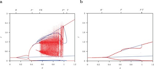
Figure 5(b) gives the one-parameter bifurcation diagram for the host-vector model (1) for $\alpha =2$. For $\varphi =0$, the set of interior coexistence equilibria is given by the curve ${\mathcal{E}}^{\circ }$, parametrized by $V_1,V_2$. We have shown in the Appendix that ${\mathcal{E}}^{\circ }$ is a locally attracting manifold. Increasing the values $\varphi >0$ the unique interior equilibrium $E^{\mathrm{int}}$ becomes unstable at the Hopf bifurcation $H^{-}$. Above this Hopf bifurcation the limit cycle is stable and the maximum and minimum values are shown in Figure 5(b). Further continuation gives a stable limit cycle which becomes unstable at a pitchfork bifurcation P. At this point, two new stable limit cycles originate. In reverse order, it occurs at a second pitchfork bifurcation P. At $\varphi =0.8$ the unstable limit cycle is symmetric (shown in Figure 6(a)). The pairs of two stable S-conjugate limit cycles are shown in Figure 6(b).

Figure 6. (a) Infected classes $I_1(t)$ (red), $I_2(t)$ (blue) unstable symmetric solutions for the limit cycle with parameter values $\alpha =2$, $\varphi =0.8$, B = 52 and normalized time for one period. (b) Infected classes $I_1^1(t_1)$ (red), $I_2^1(t_1)$ (blue) and $I_1^2(t_2)$ (green), $I_2^2(t_2)$ (pink) solutions for the two stable S-conjugate limit cycles.

No chaotic attractors exist for the host-vector model in the relevant region in the parameter space studied for $\varphi <1$. This results from the non-existence of a torus bifurcation such as in the host-only model (A1) with temporary cross-immunity for the second strain infection [2].

Under the assumption of equal host infectivity in a primary and secondary infection, we employ the parameter $B\equiv B_1=B_2$ as a bifurcation parameter. In Figures 7–9, we compare the bifurcation structure of the full model (1) with that of the QSSA model for some values $\varphi \in (0,1)$. We plot the combinations of pairs $(B,\vartheta )$ such that (a) ${\mathcal{R}}_0=1$, (b) a Hopf bifurcation or (c) a pitchfork bifurcation occurs in (1) and its QSSA counterpart in Figures 7–9. These bifurcation diagrams find application, in particular, for evaluation of control strategies which act on the vector-to-host and host-to-vector transmission of the virus, based potentially on application of anti-mosquito repellents [3,36].

Figure 7. Two-parameter $(B,\vartheta )$ bifurcation diagram with parameter $\varphi =0.2$ of (a) the system (1), and (b) the QSSA system where the fast variables $V_1,V_2$ are assumed to be in steady state (9(9a) $\begin{array}{rl}{V}_1& =\frac{\vartheta M(I_1+\varphi I_{21})}{\vartheta (I_1+I_2+\varphi (I_{21}+I_{12}))+\nu N},\end{array}$(9a) ). TC curve is for values ${\mathcal{R}}_0=1$. Left of TC there is stable disease-free equilibrium where I = 0. Between the TC and H curve, there is a stable endemic equilibrium, and beyond H, there is a stable limit cycle. No pitchfork bifurcation P is observed in this parameter region.

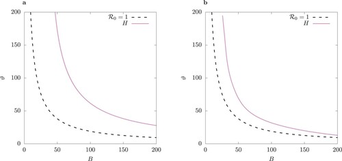
Figure 8. Two-parameter $(B,\vartheta )$ bifurcation diagram with parameter $\varphi =0.5$ of (a) the system (1), and (b) the QSSA system where the fast variables $V_1,V_2$ are assumed to be in steady state (9(9a) $\begin{array}{rl}{V}_1& =\frac{\vartheta M(I_1+\varphi I_{21})}{\vartheta (I_1+I_2+\varphi (I_{21}+I_{12}))+\nu N},\end{array}$(9a) ). TC curve is for values ${\mathcal{R}}_0=1$. Left of TC there is stable disease-free equilibrium where I = 0. Between the TC and H curve there is a stable endemic equilibrium, and between H and P, there is a stable limit cycle. Inside the region bordered by P, there is bistablity: a pair of S-symmetric limit cycles.

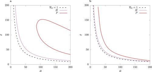
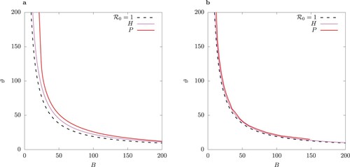
Figure 9. Two-parameter $(B,\vartheta )$ bifurcation diagram with parameter $\varphi =0.8$ of (a) the system (1), and (b) the QSSA system where the fast variables $V_1,V_2$ are assumed to be in steady state (9(9a) $\begin{array}{rl}{V}_1& =\frac{\vartheta M(I_1+\varphi I_{21})}{\vartheta (I_1+I_2+\varphi (I_{21}+I_{12}))+\nu N},\end{array}$(9a) ). TC curve is for values ${\mathcal{R}}_0=1$. Left of TC there is stable disease-free equilibrium where I = 0. Between the TC and H curve, there is a stable endemic equilibrium, and between H and P, there is a stable limit cycle. Inside the region bordered by P, there is bistablity: a pair of S-symmetric limit cycles.

The curve for $(B,\vartheta )$ where an interior equilibrium appears is computed from ${\mathcal{R}}_0=1$ using (4(4) ${\mathcal{R}}_0=\frac{B_1\vartheta }{\nu \overline{\gamma }}.$(4) ). A Hopf bifurcation leads to the appearance of a symmetric limit cycle. The pairs $(B,\vartheta )$ where the Hopf bifurcation occurs are computed numerically by finding pairs of complex conjugate eigenvalues with zero real part of the Jacobian evaluated at the interior, two-strain equilibrium $E^{\mathrm{int}}$.

We observe that the QSSA model undergoes a Hopf bifurcation for values $(B,\vartheta )$ which are closer to the values for the transcritical bifurcation TC than the full model. Also the band of stability in $(B,\vartheta )$ -space of the resulting limit cycle in the QSSA model is much narrower for a given ϕ and beyond that it becomes unstable due to a pitchfork bifurcation.

Observe that as $\varphi \to 1$, the border of the Hopf region in the host-vector model (1) approaches the TC point (Figure 9(a)). As ϕ increases, the limit cycle in the QSSA model rather quickly becomes unstable (Figure 9(b)), leading to a pair of S-conjugate limit cycles (compare Figure 11(b) versus 10(b)).

Figure 10. One-parameter bifurcation diagram for B for the case of equal infection rates $B_1=B_2=B$ in the host-vector model (1) (column (a)), and the QSSA model (column (b)). Solid lines indicate stable and dashed lines unstable solutions. Above the Hopf bifurcation point the minima and maxima for limit cycles are shown for total infected I for $\varphi =0.5$.

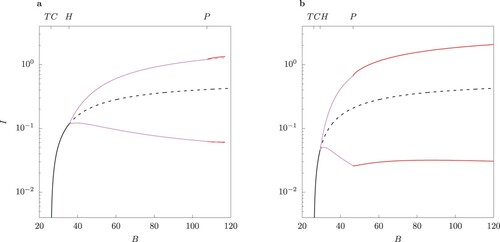
Figure 11. One-parameter bifurcation diagram for B for the case of equal infection rates $B_1=B_2=B$ in the host-vector model (1) (column (a)) and the QSSA model (column (b)). Solid lines indicate stable and dashed lines unstable solutions. Above the Hopf bifurcation point the minima and maxima for limit cycles are shown for total infected I for $\varphi =0.8$.

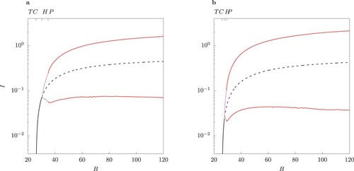
The bifurcation structure of the solutions for the host-vector model and its QSSA counterpart is examined in more detail in Figures 10–11 by varying the bifurcation parameter B and for two values of ϕ. Beyond the Hopf point H the steady state becomes unstable and a limit cycle emerges. Because of the ${\mathbb{Z}}^2$-symmetry of these two systems, S-conjugate limit cycles are possible (for more details see the two-strain model of [23]). After H with increasing B the limit cycle loses stability via a pitchfork bifurcation P. A pair of S-conjugate limit cycles emerges beyond P. Details on the minima and maxima for the two classes of primary infected $I_1,I_2$ are shown in online Appendix (Figure F2 and F3).

Introduction of control measures such as personal protection by means of repellents or repellent-treated clothing changes the parameter B. The numerical bifurcation analysis shown in Figures 10–11 reveal that changing B could lead to a switch of regime from periodic oscillations to stable equilibrium depending on the efficacy of the control. Thus, for the chosen parameter values, peak values of infected individuals may decrease by an order of magnitude

(Figure 11(a)). Sensitivity analysis is a key tool in the study of model responses to changes in conditions, see [36]. The starting point of a sensitivity analysis is the calculation of the local sensitivities of all paramters involved to quantify their contribution to changes in the model output. This gives here a method to assess which parameters gives the most effective control mechanism here to reach a situation where ${\mathcal{R}}_0<1$.

For larger values of ϕ which satisfy the conditions of Proposition 3.8, case B, namely, ${\varrho }_2<B<{\varrho }_1$ and $c_1^2-4c_0{c}_2>0$, we observe from numerical experiments that the transcritical bifurcation at ${\mathcal{R}}_0=1$ is catastrophic.

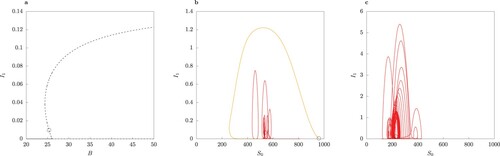
Figure 12(a) demonstrates the stability of the two-strain endemic equilibria for $\varphi =3$ as B varies. A pair of two locally asymptotically unstable equilibria for ${\mathcal{R}}_0<1$ appears. Observe that in this range the host-vector model (1) displays traits of an excitable system (Figure 12(b)). In other words, introduction of a small number of infected individuals in the population leads to a long trajectory in the phase space, which represents a transient epidemic, converging to extinction (orange trajectory in Figure 12(b)). If the initial condition is in the vicinity of the unstable limit cycle, the system displays an oscillatory behaviour before converging to the disease-free equilibrium (red trajectory in Figure 12(b)).

Figure 12. (a) One-parameter bifurcation diagram in B for the case $B_1=B_2=B$ when $\varphi =3$. Observe that in the range where two interior equilibria occur, both are locally asymptotically unstable. The dot ° marks the value of B where the two-strain equilibrium undergoes a subcritical Hopf bifurcation. (b) Phase portrait for B = 25.6 for two trajectories starting near the two unstable equilibria, marked by a dot °. The orange curve shows an epidemic with a single peak, later converging to extinction. Observe the oscillatory behaviour in the vicinity of the unstable limit cycle (red curve). c Phase portrait for B = 39.979. The trajectory follows an irregular regime.

Note that whenever ${\mathcal{R}}_0>1$, the trivial disease-free equilibrium is unstable and the border equilibria ${\mathcal{E}}_i,i=1,2$ are saddle points as well (Proposition 3.4). The numerical stability analysis shows the endemic equilibrium undergoes a subcritical Hopf bifurcation due to a pair of conjugate complex eigenvalues (marked by the dot in Figure 12(a)). The arising limit cycle is locally asymptotically unstable, as well as the coexistence equilibrium. Since any trajectory starting within Ω remains within Ω, periodic or chaotic behaviour is possible for larger values of ϕ and values of B such that ${\mathcal{R}}_0>1$. Example of chaotic behaviour is shown in Figure 12 (c).

We recall that the dengue models in [4,18] include multi-strain interactions via ADE but without a temporary cross immunity period. They show deterministic chaos when strong infectivity on secondary infection was assumed: namely, for $\varphi \approx 3$. In [22] and in the host-vector model (1) considered here, we see a similar behaviour for large ϕ values.

We look next into more detail at the effect of ϕ. In Figure 13(a), the bifurcation diagram with $\alpha =52$ is shown. These results for the host-only model has been discussed in [22]. Note that the value $\alpha =52$ corresponds to an average period of temporary cross-immunity of approximately 1 week.

Figure 13. One-parameter diagram for ϕ where $\alpha =52$ and B = 52. Equilibria or maximum and minimum values for limit cycles for total infected I for (a) the host-only model [22] and (b) the host-vector model (1). Red indicates stable and blue unstable solutions.

The results for $\alpha =52$ plotted in Figure 13(b) show that the host-vector model (1) exhibits chaos around $\varphi =2.8$. Here the chaotic region starts at the supercritical Hopf bifurcation $H^{-}$. We remark that the first Lyapunov coefficient at this bifurcation is almost zero because it is close to the Bautin bifurcation GH, Table 2. This results in the explosion of the amplitude of the resulting dynamics stable which directly governs the chaotic dynamics of the autonomous system near the Hopf bifurcation.

Finally, we present some simulations comparing the reduced models obtained via the geometric singular perturbation theory outlined in Section 4. We explore various parameter regimes for the full model (1), the QSSA model (1) with (9(9a) $\begin{array}{rl}{V}_1& =\frac{\vartheta M(I_1+\varphi I_{21})}{\vartheta (I_1+I_2+\varphi (I_{21}+I_{12}))+\nu N},\end{array}$(9a) ), and the model (1) with asymptotic expansion of the fast variables $V_i,i=1,2$ to order ε given by (12(12a) $\begin{array}{rl}{V}_1& =f(S_j,I_j,R_j,I_{12},I_{21},\epsilon )=f_0(S_j,I_j,R_j,I_{12},I_{21})+\epsilon f_1(S_j,I_j,R_j,I_{12},I_{21})\\ & +{\epsilon }^2{f}_2(S_j,I_j,R_j,I_{12},I_{21})+\dots ,\end{array}$(12a) ).

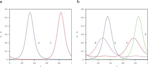
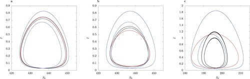
The simulations shown in Figure 14 are for illustrative purposes. The solutions in the full model for the chosen parameter values are symmetric limit cycles (Figure F1 in online Appendix). The limit cycle arises as a result of a Hopf bifurcation from the unique locally asymptotically unstable interior equilibrium $E^{\mathrm{int}}$. We compare the cycle trajectory of full model to that in the model with QSSA assumption and the approximation using asymptotic expansion for $V_i$ in Figure 14. We observe that the limit cycle for the QSSA model has a much larger amplitude in I than the other limit cycles. Further, the QSSA limit cycle in Figure 14(a–c) is S-conjugate, whereas the limit cycle in the full model is not. The second-order asymptotic expansion in ε (12(12a) $\begin{array}{rl}{V}_1& =f(S_j,I_j,R_j,I_{12},I_{21},\epsilon )=f_0(S_j,I_j,R_j,I_{12},I_{21})+\epsilon f_1(S_j,I_j,R_j,I_{12},I_{21})\\ & +{\epsilon }^2{f}_2(S_j,I_j,R_j,I_{12},I_{21})+\dots ,\end{array}$(12a) ) for $\epsilon =0.1,0.5$ (Figure 14(a–b)) gives a somewhat better approximation of the limit cycle orbit than the QSSA model, which tends to overshoot significantly in amplitude (compare the time series for $I_1,I_2$ from the model simulations in Figure F1 in online Appendix).

Thus, the simulations demonstrate a trade-off between the level of complexity retained in the QSSA model and the level of accuracy in the approximation of limit cycle orbits. In particular, for the power series approximation of $V_i,i=1,2$ higher-order terms in ε have to be included because even in the simple epidemiological model [27] the first-order asymptotic expansion did not always give a high accuracy. Of course, these numerical experiments serve for illustration of the different approaches to dimension reduction.

Figure 14. Plot of the limit cycle trajectory. Colour coding: full model (red), QSSA model (blue), asymptotic expansion to second order in ε (black). Parameter values listed in Table 1 and (a) $B_{1,2}=50,\alpha =2,\varphi =0.5,\epsilon =0.1$, (b) $B_{1,2}=50,\alpha =2,\varphi =0.5,\epsilon =0.5$, and (c) $B_{1,2}=100,\alpha =2,\varphi =0.5,\epsilon =1$.

5.2. Results for non-autonomous systems

Here we discuss the model under the assumption of a seasonally varying vector population in time which is due to seasonally changing climate factors such as temperature or rainfall that affect the vector's breeding pattern. We model the changing population as periodic forcing (3(3) $M=M(t)=M_0(1+\eta \cos \omega (t+\phi )).$(3) ) which adds essentially one new dimension to the system. This means that equilibria become limit cycles, limit cycles dynamics on an invariant torus, either limit cycles, periodic solution or quasiperiodic solutions [25].

Figure 15 (and the enlarged portion near the origin in Figure 15(b)) for the non-autonomous system (1) and (3(3) $M=M(t)=M_0(1+\eta \cos \omega (t+\phi )).$(3) ) look similar to Figure 3(b) for the autonomous system (1), however, note the torus bifurcation instead of the Hopf bifurcation because of the seasonal forcing of the mosquito population.

Figure 15. Two-strain non-autonomous host-vector model (1) and (3(3) $M=M(t)=M_0(1+\eta \cos \omega (t+\phi )).$(3) ) with B = 52. Torus bifurcation TR bifurcation exist at the same position as the Hopf H for the autonomous system (1), shown in Figure 3(b). L: limit cycle, C: complex dynamics. Details for the range $(\varphi ,\alpha )\in \{(0,1.3)\times (0,7)\}$ are shown enlarged in b.

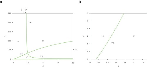
Figure 16 is the one-parameter ϕ diagram where $\alpha =2$. There is chaos above the torus bifurcation TR. Remarkably the shape of the chaotic attractor changes when the value of the Pitchfork bifurcation P from Figure 16 of the autonomous system is crossed. For the limit cycle case, there the limit cycle goes from a symmetric limit cycle in Figure 6(a) to S-conjugate limit cycle in Figure 6(b). There are no periodic solutions but obviously the chaotic solution shows the same change of type of solution of a ${\mathbb{Z}}^2$-symmetric system.

Figure 16. Two-strain non-autonomous (a) host-only model (A1) and (b) host-vector model (1) with parameter $\alpha =2$, with $\beta =104$ and $B=52$ respectively. For model (1) in forcing function (3) $M_0=10000$ and $\eta =0.1$ and in asimilar way for model (A1) in the forcing function in [2], Equation (2) ${\beta }_0=104$ and $\eta =0.5$. The bullets in (b) mark the globalmaximum and minimum values for limit cycles for total infected I. Red indicates stable and blue unstable solutions.

These results from the numerical bifurcation analysis indicate the importance of seasonal fluctuations in the vector population dynamics for $\varphi \approx 1$, leading to the emergence of a chaotic regime in correspondance with the irregular yearly spikes in dengue haemorrhagic fever incidence reported from Thailand [2]. For the autonomous model, the value $\varphi \gg 1$ is also associated with chaotic behaviour (Figures 12 and 13(b)), but in real-world scenarios such values would not be realistic. The value $\varphi \approx 1$ means that the likelihood in host-to-vector transmission of the dengue virus is equal for the primary and secondary infections, while the value $\varphi \gg 1$ that can also lead to chaotic behaviour is linked with increased likelihood for secondary infections. A value $\varphi \gg 1$ would imply that secondary infected hosts are more likely to transmit the virus to mosquitos, yet many such individuals may end up hospitalized or under home observation, and contribute less to the overall force of infection [33].

To summarize, our numerical results demonstrate that the model presented in this work possesses a simpler dynamic structure compared to models in [1,22,23] if hosts with a secondary infection have on average a lower contribution to the overall force of infection upon mosquitos than hosts with a primary infection and if no seasonality of the total vector population is taken into account. Deterministic chaos appears only under the assumption that if hosts with a secondary infection have on average a much higher contribution to the overall force of infection upon mosquitos than hosts with a primary infection. This at first may be surprising due to time series data on dengue haemorrhagic fever incidence reported from Thailand [2] that resemble chaotic behaviour. However, if we include ecological considerations such as seasonal fluctuations into the vector population, the parameter space exhibits regions with deterministic chaos which fits into the context of irregular yearly spikes in the incidence of dengue haemorrhagic fever.

This heuristic approach leads us to the conclusion that inclusion of vector ecology in the model for a vector-borne disease is essential for understanding the complexity and should be considered in models that aim at studying various approaches for control and reduction of the disease burden. Of course, climate parameters do not follow a perfectly regular short-term trend anywhere on Earth, but the longer term climate pattern holds a trend, so the sesonality effect on the vector remains more regular and predictable to a degree, as noted in [19]. Hence, in order to achieve gains in reducing the disease burden, efforts should be directed at examining the interplay of control measures efficacy and the long-term seasonal changes in the vector population. This is important especially for control based on personal protection or treatment of homes and working spaces with targeted release of repellents or insecticides.

6. Conclusion

Often the use of dimension reduction (host-only instead of host-vector) is motivated in order to obtain a model which is numerically better tractable because the time-scale difference between the host and vector yields a stiff ODE system (see [27]). However, use of sufficiently robust numerical techniques allows us to analyse both host-only and host-vector with the same numerical methods.

From the viewpoint of control strategies for vector-borne diseases, we have to incorporate the vector mosquito population in the modelling and to study its impact on the dynamics. In this study, we have included epidemiological factors such as temporary cross-immunity between strains and likelihood of host-to-vector transmission of the dengue virus. In contrast to the model of [15], our model (1) allows for long-term or periodic co-circulation of the two dengue virus strains, which is confirmed by data sets on dengue fever from Thailand.

We have compared the dynamic behaviour of models based on different approaches to dimension and complexity reduction of the full epidemiological model (1): one given by a QSSA for the fast variables and another on an asymptotic expansion based on the theory of geometric singular perturbation. The second-order asymptotic expansion gives a better approximation of the limit cycle orbits for some parameter values than the QSSA model, which tends to overshoot significantly in amplitude (compare the time series for the classes with primary infection from the model simulations in online Appendix Figure F1). When we compare the performance of the asymptotic expansion approximation of this two-strain dengue model to that in the single-strain SIR model [27], we notice that robustness and approximation in each model depends on the order of the truncation. This approach for dimension reduction should be handled carefully in applications after studying the quality of approximation and the complexity involved in computing the higher-order coefficients.

Comparison of bifurcation structures of the full epidemiological model (1) and the host-only model (A1) reveals that the autonomous host-vector system has less complex dynamics. Only stable and unstable equilibria and stable and unstable limit cycles are involved for $\varphi <1$. Deterministic chaos occurs from a catastrophic transcritical bifurcation when $\varphi \gg 1$, but such large values may be difficult to motivate in real-world applications. Torus bifurcations were not found in our study in the host-vector autonomous system (1) in the region we are interested in, and neither was chaos.

For the non-autonomous, host-vector system chaotic dynamics occurs for $\varphi <1$ as in the case of the non-autonomous host-only system via the Ruelle-Takens-Newhouse route to chaos. However, it originates now from a torus bifurcation were the period is fixed by the forcing namely 1 y${}^{-1}$ while in the host-only model it was free and described by the dynamics on the limit cycle where the torus bifurcation occurs.

We remark that in real-world applications the dengue epidemic dynamics is yearly periodical due to periodicity in the mosquito vector populations. Our analysis leads us to the conclusion that incorporating vector population dynamics in the model for a vector-borne disease is essential for understanding the dynamic complexity and should be an ingredient in models that aim at studying various approaches for control and reduction of the disease burden. However, validation of the models against disease data depends on the depth of the available data sets; in particular, more light needs to be shed on the role of asymptomatic dengue carriers in the epidemiological dynamics because such numbers are not easy to estimate [13]. The bifurcation analysis suggests that with a repellent effect that reduces sufficiently the infection rate per vector, it is possible to stabilise the oscillatory behaviour of the model. This in turn might make the disease more manageable for the healthcare system in the long term as the numbers of infected seeking hospitalization would be less variable in time. As future work, we will use the developed epidemiological model and results from the stability analysis and numerical bifurcation to evaluate the efficacy of control measures against dengue. Such include vaccination and vector control by application of insecticides, repellents and potential release of genetically modified mosquitos [8].

Acknowledgements

This publication is based upon work from COST Action CA16227 Investigation & Mathematical Analysis of Avant-garde Disease Control via Mosquito Nano-Tech-Repellents, supported by COST (European Cooperation in Science and Technology). Weblink: www.cost.eu.

Disclosure statement

No potential conflict of interest was reported by the authors.

Additional information

Funding

Rashkov is partially supported by the National Scientific Program Information and Communication Technologies for a Single Digital Market in Science, Education and Security (IKTvNOS) [contract number DO1-205/23.11.2018], financed by the Ministry of Education and Science in Bulgaria. This work was also supported by COST, European Cooperation in Science and Technology [grant number CA16227].

Appendices

Appendix 1. Host-only Model

The two-strain host-only model from [1,2] is given by the system (A1a) $\begin{array}{rl}\frac{\mathrm{d}}{\mathrm{d}t}{S}_0& =-\frac{{\beta }_1}{N}{S}_0(I_1+I_2+\varphi (I_{12}+I_{21}))+\mu (N-S_0)\end{array}$(A1a) (A1b) $\begin{array}{rl}\frac{\mathrm{d}}{\mathrm{d}t}{I}_1& =\frac{{\beta }_1}{N}{S}_0(I_1+\varphi I_{21})-(\gamma +\mu )I_1\end{array}$(A1b) (A1c) $\begin{array}{rl}\frac{\mathrm{d}}{\mathrm{d}t}{I}_2& =\frac{{\beta }_1}{N}{S}_0(I_2+\varphi I_{12})-(\gamma +\mu )I_2\end{array}$(A1c) (A1d) $\begin{array}{rl}\frac{\mathrm{d}}{\mathrm{d}t}{I}_{12}& =\frac{{\beta }_2}{N}{S}_1(I_2+\varphi I_{12})-(\gamma +\mu )I_{12}\end{array}$(A1d) (A1e) $\begin{array}{rl}\frac{\mathrm{d}}{\mathrm{d}t}{I}_{21}& =\frac{{\beta }_2}{N}{S}_2(I_1+\varphi I_{21})-(\gamma +\mu )I_{21}\end{array}$(A1e) (A1f) $\begin{array}{rl}\frac{\mathrm{d}}{\mathrm{d}t}{S}_1& =\alpha R_1-\mu S_1-\frac{{\beta }_2}{N}{S}_1(I_2+\varphi I_{12})\end{array}$(A1f) (A1g) $\begin{array}{rl}\frac{\mathrm{d}}{\mathrm{d}t}{S}_2& =\alpha R_2-\mu S_2-\frac{{\beta }_2}{N}{S}_2(I_1+\varphi I_{21})\end{array}$(A1g) (A1h) $\begin{array}{rl}\frac{\mathrm{d}}{\mathrm{d}t}{R}_1& =\gamma I_1-(\alpha +\mu )R_1\end{array}$(A1h) (A1i) $\begin{array}{rl}\frac{\mathrm{d}}{\mathrm{d}t}{R}_2& =\gamma I_2-(\alpha +\mu )R_2\end{array}$(A1i) (A1j) $\begin{array}{rl}\frac{\mathrm{d}}{\mathrm{d}t}R& =\gamma (I_{12}+I_{21})-\mu R.\end{array}$(A1j)

Appendix 2. Solving for the exclusion equilibrium ${\mathcal{E}}_1$

Setting the right-hand side of (1) equal to 0 yields $\begin{array}{rl}{I}_2^{\ast }& =\frac{B_1}{M(\gamma +\mu )}{S}_{01}^{\ast }{V}_2^{\ast },\\ R_2^{\ast }& =\frac{\gamma }{\overline{\alpha }}{I}_2^{\ast }=\frac{\gamma }{\overline{\alpha }}\frac{B_1}{M(\gamma +\mu )}{S}_{01}^{\ast }{V}_2^{\ast },\\ S_2^{\ast }& =\frac{\alpha }{\mu }{R}_2^{\ast }=\frac{\alpha }{\mu }\frac{\gamma }{\overline{\alpha }}\frac{B_1}{M(\gamma +\mu )}{S}_{01}^{\ast }{V}_2^{\ast }.\end{array}$Further, we have the following linear system in $x=S_{01}^{\ast },y=S_{01}^{\ast }{V}_2^{\ast }$, $\begin{array}{rl}N& =x+\frac{B_1}{\mu M}y\\ \nu & =\frac{\vartheta }{N}\frac{B_1}{\gamma +\mu }x-\frac{\vartheta }{N}\frac{B_1}{M(\gamma +\mu )}y\end{array}$which can be solved explicitly via algebraic manipulation and gives the corresponding equilibrium values for ${\mathcal{E}}_1$.

Appendix 3. Jacobian matrices

The Jacobian matrices used in the local stability analysis of steady states are (A3) $\begin{array}{rl}{J}_0& =\left[\begin{array}{ccccccccccc}-\mu & 0& 0& 0& 0& 0& 0& 0& 0& -B_1& -B_1\\ 0& -\overline{\gamma }& 0& 0& 0& 0& 0& 0& 0& B_1& 0\\ 0& 0& -\overline{\gamma }& 0& 0& 0& 0& 0& 0& 0& B_1\\ 0& 0& 0& -\overline{\gamma }& 0& 0& 0& 0& 0& 0& 0\\ 0& 0& 0& 0& -\overline{\gamma }& 0& 0& 0& 0& 0& 0\\ 0& 0& 0& 0& 0& -\mu & 0& \alpha & 0& 0& 0\\ 0& 0& 0& 0& 0& 0& -\mu & 0& \alpha & 0& 0\\ 0& \gamma & 0& 0& 0& 0& 0& -\overline{\alpha }& 0& 0& 0\\ 0& 0& \gamma & 0& 0& 0& 0& 0& -\overline{\alpha }& 0& 0\\ 0& {\displaystyle \frac{\vartheta }{N}}M& 0& {\displaystyle \frac{\varphi \vartheta }{N}}M& 0& 0& 0& 0& 0& -\nu & 0\\ 0& 0& {\displaystyle \frac{\vartheta }{N}}M& 0& {\displaystyle \frac{\varphi \vartheta }{N}}M& 0& 0& 0& 0& 0& -\nu \end{array}\right].\end{array}$(A3) (A4) $\begin{array}{rl}{J}_1& =[\begin{array}{ccccc}-\mu -{\displaystyle \frac{B_1{V}_2^{\ast }}{M}}& 0& 0& 0& 0\\ 0& -\overline{\gamma }& 0& 0& 0\\ {\displaystyle \frac{B_1{V}_2^{\ast }}{M}}& 0& -\overline{\gamma }& 0& 0\\ 0& 0& 0& -\overline{\gamma }& 0\\ 0& 0& 0& 0& -\overline{\gamma }\\ 0& 0& 0& 0& 0\\ 0& 0& 0& 0& 0\\ 0& \gamma & 0& 0& 0\\ 0& 0& \gamma & 0& 0\\ 0& {\displaystyle \frac{\vartheta (M-V_2^{\ast })}{N}}& 0& {\displaystyle \frac{\varphi \vartheta (M-V_2^{\ast })}{N}}& 0\\ 0& 0& {\displaystyle \frac{\vartheta (M-V_2^{\ast })}{N}}& 0& {\displaystyle \frac{\varphi \vartheta (M-V_2^{\ast })}{N}}\end{array}\\ & \begin{array}{cccccc}0& 0& 0& 0& -{\displaystyle \frac{B_1{S}_0^{\ast }}{M}}& -{\displaystyle \frac{B_1{S}_0^{\ast }}{M}}\\ 0& 0& 0& 0& {\displaystyle \frac{B_1{S}_0^{\ast }}{M}}& 0\\ 0& 0& 0& 0& 0& {\displaystyle \frac{B_1{S}_0^{\ast }}{M}}\\ 0& 0& 0& 0& {\displaystyle \frac{B_2{S}_2^{\ast }}{M}}& 0\\ {\displaystyle \frac{B_2}{M}}{V}_2^{\ast }& 0& 0& 0& 0& 0\\ -\mu -{\displaystyle \frac{B_2{V}_2^{\ast }}{M}}& 0& \alpha & 0& 0& 0\\ 0& -\mu & 0& \alpha & -{\displaystyle \frac{B_2{S}_2^{\ast }}{M}}& 0\\ 0& 0& -\overline{\alpha }& 0& 0& 0\\ 0& 0& 0& -\overline{\alpha }& 0& 0\\ 0& 0& 0& 0& -\nu & 0\\ 0& 0& 0& 0& 0& -\nu -{\displaystyle \frac{\vartheta I_2^{\ast }}{N}}\end{array}].\end{array}$(A4) with $U=M-V_1-V_2$.

Appendix 4. Proofs

A.1. Proof of proposition 3.1

The Jacobian $J_0$ of the right-hand side of (1) (see Appendix) evaluated at ${\mathcal{E}}_0$ has eigenvalues $-\mu ,-\overline{\gamma },-\overline{\alpha }$ (counted with multiplicity) as well as the eigenvalues of the $4\times 4$-minor $\left[\begin{array}{cccc}-\overline{\gamma }& 0& B_1{\displaystyle \frac{N}{M}}& 0\\ 0& -\overline{\gamma }& 0& B_1{\displaystyle \frac{N}{M}}\\ \vartheta {\displaystyle \frac{M}{N}}& 0& -\nu & 0\\ 0& \vartheta {\displaystyle \frac{M}{N}}& 0& -\nu \end{array}\right],$which are the roots λ of the polynomial (A5) ${\lambda }^2+\lambda (\overline{\gamma }+\nu )+\nu \overline{\gamma }-B_1\vartheta =0.$(A5) Polynomial (A5(A5) ${\lambda }^2+\lambda (\overline{\gamma }+\nu )+\nu \overline{\gamma }-B_1\vartheta =0.$(A5) ) has a positive real root if the free term is negative, a condition equivalent to ${\mathcal{R}}_0>1$. Hence, ${\mathcal{E}}_0$ is locally asymptotically unstable if the above condition is met.

A.2. Proofs of proposition 3.6 and 3.7

Let $x_i=B_1\frac{V_i}{M},i=1,2,q=\frac{B_2}{B_1}$. Then at the interior equilibrium (A6a) $\begin{array}{rl}{S}_0& =\frac{\mu N}{\mu +x_1+x_2},\end{array}$(A6a) (A6b) $\begin{array}{rl}{I}_1& =\frac{\mu N{x}_1}{\overline{\gamma }(\mu +x_1+x_2)},I_2=\frac{\mu N{x}_2}{\overline{\gamma }(\mu +x_1+x_2)},\end{array}$(A6b) (A6c) $\begin{array}{rl}{R}_1& =\frac{\gamma }{\overline{\alpha }}{I}_1,R_2=\frac{\gamma }{\overline{\alpha }}{I}_2,\end{array}$(A6c) (A6d) $\begin{array}{rl}{S}_1& =\frac{\alpha \gamma \mu N{x}_1}{\overline{\alpha }\overline{\gamma }(\mu +q{x}_2)(\mu +x_1+x_2)},\end{array}$(A6d) (A6e) $\begin{array}{rl}{S}_2& =\frac{\alpha \gamma \mu N{x}_2}{\overline{\alpha }\overline{\gamma }(\mu +q{x}_1)(\mu +x_1+x_2)}\end{array}$(A6e) (A6f) $\begin{array}{rl}{I}_{12}& =\frac{\alpha \gamma \mu Nq{x}_1{x}_2}{\overline{\alpha }{\overline{\gamma }}^2(\mu +q{x}_2)(\mu +x_1+x_2)},\end{array}$(A6f) (A6g) $\begin{array}{rl}{I}_{21}& =\frac{\alpha \gamma \mu Nq{x}_1{x}_2}{\overline{\alpha }{\overline{\gamma }}^2(\mu +q{x}_1)(\mu +x_1+x_2)}.\end{array}$(A6g)

Substituting the equilibrium values for the infected classes into the vectors (1j(1j) $\begin{array}{rl}\frac{\mathrm{d}}{\mathrm{d}t}{V}_1& =\frac{\vartheta }{N}(M-V_1-V_2)(I_1+\varphi I_{21})-\nu V_1\end{array}$(1j) )–(1k(1k) $\begin{array}{rl}\frac{\mathrm{d}}{\mathrm{d}t}{V}_2& =\frac{\vartheta }{N}(M-V_1-V_2)(I_2+\varphi I_{12})-\nu V_2\end{array}$(1k) ), we have to solve the nonlinear system $\begin{array}{rl}& \vartheta (B_1-x_1-x_2)(\frac{\mu x_1}{\overline{\gamma }(\mu +x_1+x_2)}+\frac{\varphi \alpha \gamma \mu q{x}_1{x}_2}{\overline{\alpha }{\overline{\gamma }}^2(\mu +q{x}_1)(\mu +x_1+x_2)})=\nu x_1,\\ & \vartheta (B_1-x_1-x_2)(\frac{\mu x_2}{\overline{\gamma }(\mu +x_1+x_2)}+\frac{\varphi \alpha \gamma \mu q{x}_1{x}_2}{\overline{\alpha }{\overline{\gamma }}^2(\mu +q{x}_2)(\mu +x_1+x_2)})=\nu x_2.\end{array}$Dividing both sides by $x_1,x_2\ne 0$, respectively, and setting $p=\frac{\nu \overline{\alpha }{\overline{\gamma }}^2}{\vartheta \mu }>0,$we arrive to the equivalent system $\begin{array}{rl}& (B_1-x_1-x_2)(\frac{\overline{\alpha }\overline{\gamma }}{\mu +x_1+x_2}+\frac{\varphi \alpha \gamma q{x}_2}{(\mu +q{x}_1)(\mu +x_1+x_2)})=p,\\ & (B_1-x_1-x_2)(\frac{\overline{\alpha }\overline{\gamma }}{\mu +x_1+x_2}+\frac{\varphi \alpha \gamma q{x}_1}{(\mu +q{x}_2)(\mu +x_1+x_2)})=p,\end{array}$and since the right side is not identically zero, if there exist positive solutions $(x_1,x_2)$, it must hold that $\frac{\varphi \alpha \gamma q{x}_2}{(\mu +q{x}_1)(\mu +x_1+x_2)}=\frac{\varphi \alpha \gamma q{x}_1}{(\mu +q{x}_2)(\mu +x_1+x_2)},$or $x_1=x_2=x$ when $\varphi >0$. Hence, we have shown that the interior equilibrium $E^{\mathrm{int}}$, whenever it exists, is a fixed equilibrium for $\varphi >0$. The values of the respective classes are $V_1=V_2=V_{\ast },I_1=I_2=I_{\ast },$ etc.

If $\varphi =0$, the above system is under-determined in $(x_1,x_2)$, and we solve for $x_1+x_2=\frac{\mu B_1({\mathcal{R}}_0-1)}{B_1+\mu {\mathcal{R}}_0},\text{ or }{V}_1+V_2=\frac{\mu M({\mathcal{R}}_0-1)}{B_1+\mu {\mathcal{R}}_0},S_0=\frac{N(\mu +\frac{B_1}{{\mathcal{R}}_0})}{\mu +B_1}.$and the remaining classes can be expressed accordingly using (A6(A6a) $\begin{array}{rl}{S}_0& =\frac{\mu N}{\mu +x_1+x_2},\end{array}$(A6a) ). This determines the curve ${\mathcal{E}}_0$.

Else, for $\varphi >0$ a substitution into the equation for the vector (1j(1j) $\begin{array}{rl}\frac{\mathrm{d}}{\mathrm{d}t}{V}_1& =\frac{\vartheta }{N}(M-V_1-V_2)(I_1+\varphi I_{21})-\nu V_1\end{array}$(1j) ) yields for x: $(B_1-2x)(\frac{\overline{\alpha }\overline{\gamma }}{\mu +2x}+\frac{\varphi \alpha \gamma qx}{(\mu +qx)(\mu +2x)})=p.$We must solve, equivalently, the quadratic (A7) $c_2{x}^2+c_{1}x+c_0=0$(A7) for solutions x>0, whose coefficients are given by $\begin{array}{rl}{c}_2& =-2\frac{B_2}{B_1}(\varphi \alpha \gamma +\overline{\gamma }\overline{\alpha }+\frac{\nu }{\vartheta \mu }{\overline{\gamma }}^2\overline{\alpha })\\ c_1& =\overline{\alpha }{B}_2\overline{\gamma }+\alpha B_2\gamma \varphi -2\overline{\alpha }\overline{\gamma }\mu -(2+\frac{B_2}{B_1})\frac{\nu }{\vartheta }{\overline{\gamma }}^2\overline{\alpha }\\ c_0& =\mu \overline{\gamma }\overline{\alpha }(B_1-\frac{\nu }{\vartheta }\overline{\gamma }).\end{array}$We examine the number of positive roots of (A7(A7) $c_2{x}^2+c_{1}x+c_0=0$(A7) ).

Because the leading coefficient $c_2$ of (A7(A7) $c_2{x}^2+c_{1}x+c_0=0$(A7) ) is always negative, Vieta's rule tells us the number of positive roots depends on the signs of the other terms. In particular, Equation (A7(A7) $c_2{x}^2+c_{1}x+c_0=0$(A7) ) has exactly one positive root if and only if $\{\begin{array}{l}{c}_1<0\\ c_0>0\end{array}\text{or}\{\begin{array}{l}{c}_1>0\\ c_0>0.\end{array}$Hence, it is sufficient to have $c_0>0$. We express the relations for the signs of the coefficients $c_i$ as inequalities for $B_1,B_2$.

Whenever ${\mathcal{R}}_0>1$, or $B_1>{\varrho }_1$, we have $c_0>0$, and otherwise, $c_0<0$ if $B_1<{\varrho }_1$.

Equation (A7(A7) $c_2{x}^2+c_{1}x+c_0=0$(A7) ) has exactly two positive roots if and only if $\begin{array}{rl}& c_1>0\\ & c_0<0\\ & c_1^2-4c_0{c}_2>0.\end{array}$We note that if $B_2<\frac{2\overline{\alpha }\overline{\gamma }(\mu +{\varrho }_1)}{\overline{\alpha }\overline{\gamma }+\alpha \gamma \varphi },$$c_1<0$ for all $B_1$. Otherwise when $\begin{array}{rl}& B_2>\frac{2\overline{\alpha }\overline{\gamma }(\mu +{\varrho }_1)}{\overline{\alpha }\overline{\gamma }+\alpha \gamma \varphi }\\ & B_1>\frac{B_2\overline{\alpha }\overline{\gamma }{\varrho }_1}{(\overline{\alpha }\overline{\gamma }+\alpha \gamma \varphi )B_2-2\overline{\alpha }\overline{\gamma }(\mu +{\varrho }_1)},\end{array}$$c_1>0$ holds.

The discriminant of (A7(A7) $c_2{x}^2+c_{1}x+c_0=0$(A7) ) $\mathrm{\Delta }=0$ if the following conditions are satisfied $\begin{array}{rl}{B}_1& =[\phantom{\frac{2\sqrt{2\alpha \gamma \varphi (B_2+2\mu )(\overline{\alpha }\overline{\gamma }(\mu +{\varrho }_1)+\alpha \gamma \mu \varphi )}}{\overline{\alpha }\overline{\gamma }{B}_2{\varrho }_1}}\frac{\overline{\alpha }\overline{\gamma }(B_2+2{\varrho }_1+2\mu )+\alpha \gamma \varphi (B_2+4\mu )}{\overline{\alpha }\overline{\gamma }{B}_2{\varrho }_1}\\ & {\pm \frac{2\sqrt{2\alpha \gamma \varphi (B_2+2\mu )(\overline{\alpha }\overline{\gamma }(\mu +{\varrho }_1)+\alpha \gamma \mu \varphi )}}{\overline{\alpha }\overline{\gamma }{B}_2{\varrho }_1}]}^{-1}\end{array}$giving the boundary between the regions $\{(B_1,B_2)|\mathrm{\Delta }<0\}$ and $\{(B_1,B_2)|\mathrm{\Delta }>0\}$.

To show local stability of the curve ${\mathcal{E}}^{\circ }$ (for the case $\varphi =0$), we compute the the Jacobian at a point $\mathbf{x}\in {\mathcal{E}}^{\circ }$: $\begin{array}{rl}{J}_2(\mathbf{x})& =[\begin{array}{cccccc}-\mu -{\displaystyle \frac{B_1(V_1+V_2)}{M}}& 0& 0& 0& 0& 0\\ {\displaystyle \frac{B_1}{M}}{V}_1& -\overline{\gamma }& 0& 0& 0& 0\\ {\displaystyle \frac{B_1}{M}}{V}_2& 0& -\overline{\gamma }& 0& 0& 0\\ 0& 0& 0& -\overline{\gamma }& 0& 0\\ 0& 0& 0& 0& -\overline{\gamma }& {\displaystyle \frac{B_2}{M}}{V}_2\\ 0& 0& 0& 0& 0& -\mu -{\displaystyle \frac{B_2}{M}}{V}_2\\ 0& 0& 0& 0& 0& 0\\ 0& \gamma & 0& 0& 0& 0\\ 0& 0& \gamma & 0& 0& 0\\ 0& {\displaystyle \frac{\vartheta }{N}}U& 0& 0& 0& 0\\ 0& 0& {\displaystyle \frac{\vartheta }{N}}U& 0& 0& 0\end{array}\\ & \begin{array}{ccccc}0& 0& 0& -{\displaystyle \frac{B_1}{M}}{S}_0& -{\displaystyle \frac{B}{M}}{S}_0\\ 0& 0& 0& {\displaystyle \frac{B_1}{M}}{S}_0& 0\\ 0& 0& 0& 0& {\displaystyle \frac{B_1}{M}}{S}_0\\ {\displaystyle \frac{B_2}{M}}{V}_1& 0& 0& {\displaystyle \frac{B_2}{M}}{S}_2& 0\\ 0& 0& 0& 0& {\displaystyle \frac{B_2}{M}}{S}_1\\ 0& \alpha & 0& 0& -{\displaystyle \frac{B_2}{M}}{S}_1\\ -\mu -{\displaystyle \frac{B_2}{M}}{V}_1& 0& \alpha & -{\displaystyle \frac{B_2}{M}}{S}_2& 0\\ 0& -\overline{\alpha }& 0& 0& 0\\ 0& 0& -\overline{\alpha }& 0& 0\\ 0& 0& 0& -{\displaystyle \frac{\vartheta I_1}{N}}-\nu & 0\\ 0& 0& 0& 0& -{\displaystyle \frac{\vartheta I_2}{N}}-\nu \end{array}]\end{array}$where the entries satisfy the following: $V_1,V_2\ge 0$, such that $\begin{array}{rl}{V}_1+V_2& =\frac{M\mu ({\mathcal{R}}_0-1)}{B_1+\mu {\mathcal{R}}_0},\\ S_0& =\frac{N(\mu +\frac{B_1}{{\mathcal{R}}_0})}{\mu +B_1},U=\frac{M(\mu +B_1)}{\mu {\mathcal{R}}_0+B_1}\end{array}$and $I_i,S_i,i=1,2$ are computed from (A6(A6a) $\begin{array}{rl}{S}_0& =\frac{\mu N}{\mu +x_1+x_2},\end{array}$(A6a) ).

From $J_2$'s structure it is obvious that $-\overline{\alpha },-\overline{\gamma },-\mu -\frac{B_i}{M}{V}_i,i=1,2$ are eigenvalues (the first two have algebraic multiplicity 2). The characteristic polynomial of the remaining $5\times 5$-minor of $J_2$ is $\begin{array}{rl}p(\lambda )& ={\lambda }^5+(2\overline{\gamma }+\mu +2\nu +B_1\frac{\mu ({\mathcal{R}}_0-1)}{B_1+\mu {\mathcal{R}}_0}+\frac{\mu B_1\theta ({\mathcal{R}}_0-1)}{\overline{\gamma }(\mu +B_1){\mathcal{R}}_0}){\lambda }^4\\ & +((\overline{\gamma }+\nu {)}^2+I_1{I}_2\frac{{\theta }^2}{N^2}+2\overline{\gamma }\mu +2\mu \nu +2(\overline{\gamma }+2\nu )\frac{\mu B_1({\mathcal{R}}_0-1)}{B_1+\mu {\mathcal{R}}_0}+2\frac{\mu B_1\theta ({\mathcal{R}}_0-1)}{(\mu +B_1){\mathcal{R}}_0}\\ & +\frac{\mu B_1\theta ({\mathcal{R}}_0-1)}{\overline{\gamma }(\mu +B_1){\mathcal{R}}_0}(\mu +\nu )+\frac{{\mu }^2{B}_1^2\theta ({\mathcal{R}}_0-1{)}^2}{\overline{\gamma }(\mu +B_1){\mathcal{R}}_0(B_1+\mu {\mathcal{R}}_0)}){\lambda }^3\\ & +((\overline{\gamma }+\nu {)}^2\mu +{\overline{\gamma }}^2\frac{\mu B_1({\mathcal{R}}_0-1)}{B_1+\mu {\mathcal{R}}_0}+{\nu }^2\frac{\mu B_1({\mathcal{R}}_0-1)}{B_1+\mu {\mathcal{R}}_0}+2I_1{I}_2\overline{\gamma }\frac{{\theta }^2}{N^2}+\frac{\mu B_1\theta ({\mathcal{R}}_0-1)}{(\mu +B_1){\mathcal{R}}_0}\overline{\gamma }\\ & +I_1{I}_2\mu \frac{{\theta }^2}{N^2}+I_1{I}_2\frac{{\theta }^2}{N^2}\frac{\mu B_1({\mathcal{R}}_0-1)}{B_1+\mu {\mathcal{R}}_0}+3\overline{\gamma }\nu \frac{\mu B_1({\mathcal{R}}_0-1)}{B_1+\mu {\mathcal{R}}_0}+2\frac{\mu B_1\theta ({\mathcal{R}}_0-1)}{(\mu +B_1){\mathcal{R}}_0}\mu \\ & +\frac{\mu B_1\theta ({\mathcal{R}}_0-1)}{(\mu +B_1){\mathcal{R}}_0}\nu +\frac{\mu B_1\theta ({\mathcal{R}}_0-1)}{\overline{\gamma }(\mu +B_1){\mathcal{R}}_0}\mu \nu +\frac{2{\mu }^2{B}_1^2\theta ({\mathcal{R}}_0-1{)}^2}{(\mu +B_1){\mathcal{R}}_0(B_1+\mu {\mathcal{R}}_0)}\\ & +\frac{{\mu }^2{B}_1^2\theta \nu ({\mathcal{R}}_0-1{)}^2}{\overline{\gamma }(\mu +B_1){\mathcal{R}}_0(B_1+\mu {\mathcal{R}}_0)}){\lambda }^2\\ & +(\overline{\gamma }{\nu }^2\frac{\mu B_1({\mathcal{R}}_0-1)}{B_1+\mu {\mathcal{R}}_0}+{\overline{\gamma }}^2\nu \frac{\mu B_1({\mathcal{R}}_0-1)}{B_1+\mu {\mathcal{R}}_0}+I_1{I}_2{\overline{\gamma }}^2\frac{{\theta }^2}{N^2}+2I_1{I}_2\overline{\gamma }\frac{{\theta }^2}{N^2}\frac{\mu B_1({\mathcal{R}}_0-1)}{B_1+\mu {\mathcal{R}}_0}\\ & +\frac{{\mu }^2{B}_1^2\theta ({\mathcal{R}}_0-1{)}^2}{(\mu +B_1){\mathcal{R}}_0(B_1+\mu {\mathcal{R}}_0)}\overline{\gamma }+2I_1{I}_2\overline{\gamma }\mu \frac{{\theta }^2}{N^2}\\ & +\frac{{\mu }^2{B}_1\theta ({\mathcal{R}}_0-1)}{(\mu +B_1){\mathcal{R}}_0}\overline{\gamma }+\frac{{\mu }^2{B}_1^2\nu \theta ({\mathcal{R}}_0-1{)}^2}{(\mu +B_1){\mathcal{R}}_0(B_1+\mu {\mathcal{R}}_0)}\\ & +(I_1{V}_2+I_2{V}_1)\frac{B_1}{M}\overline{\gamma }\nu \frac{\theta }{N}+\frac{{\mu }^2\nu B_1\theta ({\mathcal{R}}_0-1)}{(\mu +B_1){\mathcal{R}}_0})\lambda \\ & +I_1{I}_2{\overline{\gamma }}^2\mu \frac{{\theta }^2}{N^2}+I_1{I}_2{\overline{\gamma }}^2\frac{{\theta }^2}{N^2}\frac{\mu B_1({\mathcal{R}}_0-1)}{B_1+\mu {\mathcal{R}}_0}+(I_2{V}_1+I_1{V}_2)\frac{B_1}{M}{\overline{\gamma }}^2\nu \frac{\theta }{N}\end{array}$where for the sake of shortness, we denote $\overline{\gamma }=\gamma +\mu$. This polynomial has only non-negative coefficients, and does not have any positive real roots. Hence, the curve ${\mathcal{E}}_0$ consists of points which are local attractors.

A.3. Proof of lemma 3.9

Note $\begin{array}{rl}& \frac{\mathrm{\partial }}{\mathrm{\partial }x}(\frac{\overline{\alpha }\overline{\gamma }}{\mu +2x}+\frac{\varphi \alpha \gamma x}{(\mu +x)(\mu +2x)})\\ & =\frac{(\varphi \alpha \gamma -2\overline{\alpha }\overline{\gamma }){\mu }^2-4\mu \overline{\alpha }\overline{\gamma }x-2(\overline{\alpha }\overline{\gamma }+\varphi \alpha \gamma )x^2}{(\mu +x{)}^2(\mu +2x{)}^2}<0,\end{array}$for the range $0<\varphi \le 2$. Hence, the existing solution x must be monotonically increasing with ϕ to maintain the equality in $(B-2x)(\frac{\overline{\alpha }\overline{\gamma }}{\mu +2x}+\frac{\varphi \alpha \gamma x}{(\mu +x)(\mu +2x)})=p,$since the solution is unique.

Since $\mu \ll \alpha ,B,\gamma$, we can approximate the solution of the equation by replacing x by $x+\mu$ into the numerator of the term on left-hand side of the equation. Then $(B-2x)(\alpha \gamma (1+\varphi ))-2p\mu =2xp,\text{with}p\approx \frac{\nu }{\vartheta \mu }\alpha {\gamma }^2,$giving (A8) $x\approx \frac{B(1+\varphi )-2\frac{\nu \gamma }{\vartheta }}{2(1+\varphi +\frac{\nu \gamma }{\vartheta \mu })}.$(A8) This means that the interior equilibrium value for the infected vector classes $V_1=V_2=\mathcal{O}(\mu )$.

A.4. Normal hyperbolicity of the set of critical points

Recall the fast system $\begin{array}{rl}\frac{\mathrm{d}}{\mathrm{d}t}{V}_1& =F_1(V_1,V_2,I)=\frac{\vartheta }{N}(M-V_1-V_2)(I_1+\varphi I_{21})-\nu V_1\\ \frac{\mathrm{d}}{\mathrm{d}t}{V}_2& =F_2(V_1,V_2,I)=\frac{\vartheta }{N}(M-V_1-V_2)(I_2+\varphi I_{12})-\nu V_2.\end{array}$The Jacobian $\frac{\mathrm{\partial }F}{\mathrm{\partial }V}{|}_{\mathcal{M}}$ of the fast system in $V_1,V_2$ on the set of critical points is given by $\frac{\mathrm{\partial }F}{\mathrm{\partial }V}{|}_{\mathcal{M}}=\left[\begin{array}{cc}-{\displaystyle \frac{\theta }{N}}(I_1+\varphi I_{21})-\nu & -\frac{\theta }{N}(I_1+\varphi I_{21})\\ -{\displaystyle \frac{\theta }{N}}(I_2+\varphi I_{12})& -\frac{\theta }{N}(I_2+\varphi I_{12})-\nu \end{array}\right].$This matrix is constant on the positive half-lines $I_2+\varphi I_{12}=l_1,I_1+\varphi I_{21}=l_2$, and the eigenvalues are ${\lambda }_1=-\nu ,{\lambda }_2=-(\nu +l_1+l_2)<-\nu .$${\lambda }_i,i=1,2$ are bounded uniformly away from the imaginary axis, which concludes the proof.

Appendix 5. Asymptotic expansion

The substitution of the power series in ε into the invariance equation (11(11) $\frac{\mathrm{d}{V}_i}{\mathrm{d}\tau }=\sum _{j=0}^2\frac{\mathrm{\partial }{V}_i}{\mathrm{\partial }{S}_j}\frac{\mathrm{d}{S}_j}{\mathrm{d}\tau }+\sum _{j=1}^2\frac{\mathrm{\partial }{V}_i}{\mathrm{\partial }{I}_j}\frac{\mathrm{d}{I}_j}{\mathrm{d}\tau }+\sum _{j=1}^2\frac{\mathrm{\partial }{V}_i}{\mathrm{\partial }{R}_j}\frac{\mathrm{d}{R}_j}{\mathrm{d}\tau }+\frac{\mathrm{\partial }{V}_i}{\mathrm{\partial }{I}_{12}}\frac{\mathrm{d}{I}_{12}}{\mathrm{d}\tau }+\frac{\mathrm{\partial }{V}_i}{\mathrm{\partial }{I}_{21}}\frac{\mathrm{d}{I}_{21}}{\mathrm{d}\tau },$(11) ) gives $\begin{array}{rl}\frac{\mathrm{d}f}{\mathrm{d}\tau }& =\sum _{j=0}^2\frac{\mathrm{\partial }f}{\mathrm{\partial }{S}_j}\frac{\mathrm{d}{S}_j}{\mathrm{d}\tau }+\sum _{j=1}^2\frac{\mathrm{\partial }f}{\mathrm{\partial }{I}_j}\frac{\mathrm{d}{I}_j}{\mathrm{d}\tau }+\sum _{j=1}^2\frac{\mathrm{\partial }f}{\mathrm{\partial }{R}_j}\frac{\mathrm{d}{R}_j}{\mathrm{d}\tau }+\frac{\mathrm{\partial }f}{\mathrm{\partial }{I}_{12}}\frac{\mathrm{d}{I}_{12}}{\mathrm{d}\tau }+\frac{\mathrm{\partial }f}{\mathrm{\partial }{I}_{21}}\frac{\mathrm{d}{I}_{21}}{\mathrm{d}\tau },\\ \frac{\mathrm{d}g}{\mathrm{d}\tau }& =\sum _{j=0}^2\frac{\mathrm{\partial }g}{\mathrm{\partial }{S}_j}\frac{\mathrm{d}{S}_j}{\mathrm{d}\tau }+\sum _{j=1}^2\frac{\mathrm{\partial }g}{\mathrm{\partial }{I}_j}\frac{\mathrm{d}{I}_j}{\mathrm{d}\tau }+\sum _{j=1}^2\frac{\mathrm{\partial }g}{\mathrm{\partial }{R}_j}\frac{\mathrm{d}{R}_j}{\mathrm{d}\tau }+\frac{\mathrm{\partial }g}{\mathrm{\partial }{I}_{12}}\frac{\mathrm{d}{I}_{12}}{\mathrm{d}\tau }+\frac{\mathrm{\partial }g}{\mathrm{\partial }{I}_{21}}\frac{\mathrm{d}{I}_{21}}{\mathrm{d}\tau }.\end{array}$Taking the expansions of f, g up to order ε produces the following system: (A9) $\begin{array}{rl}& \frac{1}{\epsilon }(\frac{\vartheta }{N}(M-f_0-\epsilon f_1-{\epsilon }^2{f}_2-g_0-\epsilon g_1-{\epsilon }^2{g}_2)(I_1+\varphi I_{21})-\nu (f_0+\epsilon f_1+{\epsilon }^2{f}_2))\\ & =\sum _{j=0}^2(\frac{\mathrm{\partial }{f}_0}{\mathrm{\partial }{S}_j}+\epsilon \frac{\mathrm{\partial }{f}_1}{\mathrm{\partial }{S}_j}+{\epsilon }^2\frac{\mathrm{\partial }{f}_2}{\mathrm{\partial }{S}_j})\frac{\mathrm{d}{S}_j}{\mathrm{d}\tau }+\sum _{j=1}^2(\frac{\mathrm{\partial }{f}_0}{\mathrm{\partial }{I}_j}+\epsilon \frac{\mathrm{\partial }{f}_1}{\mathrm{\partial }{I}_j}+{\epsilon }^2\frac{\mathrm{\partial }{f}_2}{\mathrm{\partial }{I}_j})\frac{\mathrm{d}{I}_j}{\mathrm{d}\tau }\\ & +\sum _{j=1}^2(\frac{\mathrm{\partial }{f}_0}{\mathrm{\partial }{R}_j}+\epsilon \frac{\mathrm{\partial }{f}_1}{\mathrm{\partial }{R}_j}+{\epsilon }^2\frac{\mathrm{\partial }{f}_2}{\mathrm{\partial }{R}_j})\frac{\mathrm{d}{R}_j}{\mathrm{d}\tau }+(\frac{\mathrm{\partial }{f}_0}{\mathrm{\partial }{I}_{12}}+\epsilon \frac{\mathrm{\partial }{f}_1}{\mathrm{\partial }{I}_{12}}+{\epsilon }^2\frac{\mathrm{\partial }{f}_2}{\mathrm{\partial }{I}_{12}})\frac{\mathrm{d}{I}_{12}}{\mathrm{d}\tau }\\ & +(\frac{\mathrm{\partial }{f}_0}{\mathrm{\partial }{I}_{21}}+\epsilon \frac{\mathrm{\partial }{f}_1}{\mathrm{\partial }{I}_{21}}+{\epsilon }^2\frac{\mathrm{\partial }{f}_2}{\mathrm{\partial }{I}_{21}})\frac{\mathrm{d}{I}_{21}}{\mathrm{d}\tau }+\text{ higher order terms},\\ \frac{1}{\epsilon }& (\frac{\vartheta }{N}(M-f_0-\epsilon f_1-{\epsilon }^2{f}_2-g_0-\epsilon g_1-{\epsilon }^2{g}_2)(I_2+\varphi I_{12})-\nu (g_0+\epsilon g_1+{\epsilon }^2{g}_2))\\ & =\sum _{j=0}^2(\frac{\mathrm{\partial }{g}_0}{\mathrm{\partial }{S}_j}+\epsilon \frac{\mathrm{\partial }{g}_1}{\mathrm{\partial }{S}_j}+{\epsilon }^2\frac{\mathrm{\partial }{g}_2}{\mathrm{\partial }{S}_j})\frac{\mathrm{d}{S}_j}{\mathrm{d}\tau }+\sum _{j=1}^2(\frac{\mathrm{\partial }{g}_0}{\mathrm{\partial }{I}_j}+\epsilon \frac{\mathrm{\partial }{g}_1}{\mathrm{\partial }{I}_j}+{\epsilon }^2\frac{\mathrm{\partial }{g}_2}{\mathrm{\partial }{I}_j})\frac{\mathrm{d}{I}_j}{\mathrm{d}\tau }\\ & +\sum _{j=1}^2(\frac{\mathrm{\partial }{g}_0}{\mathrm{\partial }{R}_j}+\epsilon \frac{\mathrm{\partial }{g}_1}{\mathrm{\partial }{R}_j}+{\epsilon }^2\frac{\mathrm{\partial }{g}_2}{\mathrm{\partial }{R}_j})\frac{\mathrm{d}{R}_j}{\mathrm{d}\tau }+(\frac{\mathrm{\partial }{g}_0}{\mathrm{\partial }{I}_{12}}+\epsilon \frac{\mathrm{\partial }{g}_1}{\mathrm{\partial }{I}_{12}}+{\epsilon }^2\frac{\mathrm{\partial }{g}_2}{\mathrm{\partial }{I}_{12}})\frac{\mathrm{d}{I}_{12}}{\mathrm{d}\tau }\\ & +(\frac{\mathrm{\partial }{g}_0}{\mathrm{\partial }{I}_{21}}+\epsilon \frac{\mathrm{\partial }{g}_1}{\mathrm{\partial }{I}_{21}}+{\epsilon }^2\frac{\mathrm{\partial }{g}_2}{\mathrm{\partial }{I}_{21}})\frac{\mathrm{d}{I}_{21}}{\mathrm{d}\tau }+\text{ higher order terms}.\end{array}$(A9) Collecting terms of order ${\epsilon }^{-1}$ gives the system $\begin{array}{rl}\frac{\vartheta }{N}(M-f_0-g_0)(I_1+\varphi I_{21})-\nu f_0& =0\\ \frac{\vartheta }{N}(M-f_0-g_0)(I_2+\varphi I_{12})-\nu g_0& =0\end{array}$whose solutions are the expressions of the free terms in (12(12a) $\begin{array}{rl}{V}_1& =f(S_j,I_j,R_j,I_{12},I_{21},\epsilon )=f_0(S_j,I_j,R_j,I_{12},I_{21})+\epsilon f_1(S_j,I_j,R_j,I_{12},I_{21})\\ & +{\epsilon }^2{f}_2(S_j,I_j,R_j,I_{12},I_{21})+\dots ,\end{array}$(12a) ): (A10a) $\begin{array}{rl}{f}_0& =\frac{\vartheta M(I_1+\varphi I_{21})}{\vartheta (I_1+I_2+\varphi (I_{21}+I_{12}))+\nu N},\end{array}$(A10a) (A10b) $\begin{array}{rl}{g}_0& =\frac{\vartheta M(I_2+\varphi I_{12})}{\vartheta (I_1+I_2+\varphi (I_{21}+I_{12}))+\nu N}.\end{array}$(A10b)

To find the coefficients for terms of order ${\epsilon }^0$ in (A9(A9) $\begin{array}{rl}& \frac{1}{\epsilon }(\frac{\vartheta }{N}(M-f_0-\epsilon f_1-{\epsilon }^2{f}_2-g_0-\epsilon g_1-{\epsilon }^2{g}_2)(I_1+\varphi I_{21})-\nu (f_0+\epsilon f_1+{\epsilon }^2{f}_2))\\ & =\sum _{j=0}^2(\frac{\mathrm{\partial }{f}_0}{\mathrm{\partial }{S}_j}+\epsilon \frac{\mathrm{\partial }{f}_1}{\mathrm{\partial }{S}_j}+{\epsilon }^2\frac{\mathrm{\partial }{f}_2}{\mathrm{\partial }{S}_j})\frac{\mathrm{d}{S}_j}{\mathrm{d}\tau }+\sum _{j=1}^2(\frac{\mathrm{\partial }{f}_0}{\mathrm{\partial }{I}_j}+\epsilon \frac{\mathrm{\partial }{f}_1}{\mathrm{\partial }{I}_j}+{\epsilon }^2\frac{\mathrm{\partial }{f}_2}{\mathrm{\partial }{I}_j})\frac{\mathrm{d}{I}_j}{\mathrm{d}\tau }\\ & +\sum _{j=1}^2(\frac{\mathrm{\partial }{f}_0}{\mathrm{\partial }{R}_j}+\epsilon \frac{\mathrm{\partial }{f}_1}{\mathrm{\partial }{R}_j}+{\epsilon }^2\frac{\mathrm{\partial }{f}_2}{\mathrm{\partial }{R}_j})\frac{\mathrm{d}{R}_j}{\mathrm{d}\tau }+(\frac{\mathrm{\partial }{f}_0}{\mathrm{\partial }{I}_{12}}+\epsilon \frac{\mathrm{\partial }{f}_1}{\mathrm{\partial }{I}_{12}}+{\epsilon }^2\frac{\mathrm{\partial }{f}_2}{\mathrm{\partial }{I}_{12}})\frac{\mathrm{d}{I}_{12}}{\mathrm{d}\tau }\\ & +(\frac{\mathrm{\partial }{f}_0}{\mathrm{\partial }{I}_{21}}+\epsilon \frac{\mathrm{\partial }{f}_1}{\mathrm{\partial }{I}_{21}}+{\epsilon }^2\frac{\mathrm{\partial }{f}_2}{\mathrm{\partial }{I}_{21}})\frac{\mathrm{d}{I}_{21}}{\mathrm{d}\tau }+\text{ higher order terms},\\ \frac{1}{\epsilon }& (\frac{\vartheta }{N}(M-f_0-\epsilon f_1-{\epsilon }^2{f}_2-g_0-\epsilon g_1-{\epsilon }^2{g}_2)(I_2+\varphi I_{12})-\nu (g_0+\epsilon g_1+{\epsilon }^2{g}_2))\\ & =\sum _{j=0}^2(\frac{\mathrm{\partial }{g}_0}{\mathrm{\partial }{S}_j}+\epsilon \frac{\mathrm{\partial }{g}_1}{\mathrm{\partial }{S}_j}+{\epsilon }^2\frac{\mathrm{\partial }{g}_2}{\mathrm{\partial }{S}_j})\frac{\mathrm{d}{S}_j}{\mathrm{d}\tau }+\sum _{j=1}^2(\frac{\mathrm{\partial }{g}_0}{\mathrm{\partial }{I}_j}+\epsilon \frac{\mathrm{\partial }{g}_1}{\mathrm{\partial }{I}_j}+{\epsilon }^2\frac{\mathrm{\partial }{g}_2}{\mathrm{\partial }{I}_j})\frac{\mathrm{d}{I}_j}{\mathrm{d}\tau }\\ & +\sum _{j=1}^2(\frac{\mathrm{\partial }{g}_0}{\mathrm{\partial }{R}_j}+\epsilon \frac{\mathrm{\partial }{g}_1}{\mathrm{\partial }{R}_j}+{\epsilon }^2\frac{\mathrm{\partial }{g}_2}{\mathrm{\partial }{R}_j})\frac{\mathrm{d}{R}_j}{\mathrm{d}\tau }+(\frac{\mathrm{\partial }{g}_0}{\mathrm{\partial }{I}_{12}}+\epsilon \frac{\mathrm{\partial }{g}_1}{\mathrm{\partial }{I}_{12}}+{\epsilon }^2\frac{\mathrm{\partial }{g}_2}{\mathrm{\partial }{I}_{12}})\frac{\mathrm{d}{I}_{12}}{\mathrm{d}\tau }\\ & +(\frac{\mathrm{\partial }{g}_0}{\mathrm{\partial }{I}_{21}}+\epsilon \frac{\mathrm{\partial }{g}_1}{\mathrm{\partial }{I}_{21}}+{\epsilon }^2\frac{\mathrm{\partial }{g}_2}{\mathrm{\partial }{I}_{21}})\frac{\mathrm{d}{I}_{21}}{\mathrm{d}\tau }+\text{ higher order terms}.\end{array}$(A9) ), we use the fact that many partial derivatives vanish identically $\begin{array}{rl}\frac{\mathrm{\partial }{f}_0}{\mathrm{\partial }{S}_j}& =\frac{\mathrm{\partial }{g}_0}{\mathrm{\partial }{S}_j}=0,j=0,1,2,\\ \frac{\mathrm{\partial }{f}_0}{\mathrm{\partial }{R}_j}& =\frac{\mathrm{\partial }{g}_0}{\mathrm{\partial }{R}_j}=0,j=1,2,\end{array}$which results in the vector ${\mathbf{h}}_1=\left[\begin{array}{c}{\displaystyle \frac{\mathrm{\partial }{f}_0}{\mathrm{\partial }{I}_1}(\frac{B_1}{M}{S}_0{f}_0-(\gamma +\mu )I_1)+\frac{\mathrm{\partial }{f}_0}{\mathrm{\partial }{I}_2}(\frac{B_1}{M}{S}_0{g}_0-(\gamma +\mu )I_2)\dots }\\ {\displaystyle +\frac{\mathrm{\partial }{f}_0}{\mathrm{\partial }{I}_{12}}(\frac{B_2}{M}{S}_1{g}_0-(\gamma +\mu )I_{12})+\frac{\mathrm{\partial }{f}_0}{\mathrm{\partial }{I}_{21}}(\frac{B_2}{M}{S}_2{f}_0-(\gamma +\mu )I_{21})}\\ {\displaystyle \frac{\mathrm{\partial }{g}_0}{\mathrm{\partial }{I}_1}(\frac{B_1}{M}{S}_0{f}_0-(\gamma +\mu )I_1)+\frac{\mathrm{\partial }{g}_0}{\mathrm{\partial }{I}_2}(\frac{B_1}{M}{S}_0{g}_0-(\gamma +\mu )I_2)\dots }\\ {\displaystyle +\frac{\mathrm{\partial }{g}_0}{\mathrm{\partial }{I}_{12}}(\frac{B_2}{M}{S}_1{g}_0-(\gamma +\mu )I_{12})+\frac{\mathrm{\partial }{g}_0}{\mathrm{\partial }{I}_{21}}(\frac{B_2}{M}{S}_2{f}_0-(\gamma +\mu )I_{21})}\end{array}\right]$to be used in Equation (13(13) $\mathbf{M}(f_{i+1},g_{i+1}{)}^T=-{\mathbf{h}}_i,$(13) ), and where the partial derivatives are given by $\begin{array}{rl}\frac{\mathrm{\partial }{f}_0}{\mathrm{\partial }{I}_1}& =\frac{\vartheta M(\vartheta (I_2+\varphi I_{12})+\nu N)}{(\vartheta (I_1+I_2+\varphi (I_{21}+I_{12}))+\nu N{)}^2}\\ \frac{\mathrm{\partial }{f}_0}{\mathrm{\partial }{I}_2}& =-\frac{{\vartheta }^{2}M(I_1+\varphi I_{21})}{(\vartheta (I_1+I_2+\varphi (I_{21}+I_{12}))+\nu N{)}^2}\\ \frac{\mathrm{\partial }{f}_0}{\mathrm{\partial }{I}_{21}}& =\frac{\vartheta \varphi M(\vartheta (I_2+\varphi I_{12})+\nu N)}{(\vartheta (I_1+I_2+\varphi (I_{21}+I_{12}))+\nu N{)}^2}\\ \frac{\mathrm{\partial }{f}_0}{\mathrm{\partial }{I}_{12}}& =-\frac{{\vartheta }^2\varphi M(I_1+\varphi I_{21})}{(\vartheta (I_1+I_2+\varphi (I_{21}+I_{12}))+\nu N{)}^2}\\ \frac{\mathrm{\partial }{g}_0}{\mathrm{\partial }{I}_1}& =-\frac{{\vartheta }^{2}M(I_2+\varphi I_{12})}{(\vartheta (I_1+I_2+\varphi (I_{21}+I_{12}))+\nu N{)}^2}\\ \frac{\mathrm{\partial }{g}_0}{\mathrm{\partial }{I}_2}& =\frac{\vartheta M(\vartheta (I_1+\varphi I_{21})+\nu N)}{(\vartheta (I_1+I_2+\varphi (I_{21}+I_{12}))+\nu N{)}^2}\\ \frac{\mathrm{\partial }{g}_0}{\mathrm{\partial }{I}_{21}}& =-\frac{{\vartheta }^2\varphi M(I_2+\varphi I_{12})}{(\vartheta (I_1+I_2+\varphi (I_{21}+I_{12}))+\nu N{)}^2}\\ \frac{\mathrm{\partial }{g}_0}{\mathrm{\partial }{I}_{12}}& =\frac{\vartheta \varphi M(\vartheta (I_1+\varphi I_{21})+\nu N)}{(\vartheta (I_1+I_2+\varphi (I_{21}+I_{12}))+\nu N{)}^2}.\end{array}$The coefficients $f_1,g_1$ are given by (A11a) $\begin{array}{rl}{f}_1& =-\frac{B_1{\vartheta }^{2}M\nu N^2(I_1+\varphi I_{21})S_0}{(\vartheta (I_1+I_2+\varphi (I_{21}+I_{12}))+\nu N{)}^4}+\frac{(\gamma +\mu )\vartheta M\nu N^2(I_1+\varphi I_{21})}{(\vartheta (I_1+I_2+\varphi (I_{21}+I_{12}))+\nu N{)}^3}\\ & -\frac{B_2{\vartheta }^2\varphi M(I_1+\varphi I_{21})}{(\vartheta (I_1+I_2+\varphi (I_{21}+I_{12}))+\nu N{)}^4}(2\vartheta N(I_2+\varphi I_{12})(S_2-S_1)\\ & +\frac{{\vartheta }^2}{\nu }(I_2+\varphi I_{12})(I_1+I_2+\varphi I_{21}+\varphi I_{12})(S_2-S_1)+N^2\nu S_2),\end{array}$(A11a) (A11b) $\begin{array}{rl}{g}_1& =-\frac{B_1{\vartheta }^{2}M\nu N^2(I_2+\varphi I_{12})S_0}{(\vartheta (I_1+I_2+\varphi (I_{21}+I_{12}))+\nu N{)}^4}+\frac{(\gamma +\mu )\vartheta M\nu N^2(I_2+\varphi I_{12})}{(\vartheta (I_1+I_2+\varphi (I_{21}+I_{12}))+\nu N{)}^3}\\ & -\frac{B_2{\vartheta }^2\varphi M(I_2+\varphi I_{12})}{(\vartheta (I_1+I_2+\varphi (I_{21}+I_{12}))+\nu N{)}^4}(2\vartheta N(I_1+\varphi I_{21})(S_1-S_2)\\ & +\frac{{\vartheta }^2}{\nu }(I_1+\varphi I_{21})(I_1+I_2+\varphi I_{21}+\varphi I_{12})(S_1-S_2)+N^2\nu S_1).\end{array}$(A11b)

For the second-order term, the vector ${\mathbf{h}}_2$ has entries ${\mathbf{h}}_2=\left[\begin{array}{c}{\displaystyle \frac{\mathrm{\partial }{f}_1}{\mathrm{\partial }{S}_0}(\mu (N-S_0)-\frac{B_1}{M}{S}_0(f_0+g_0))+\frac{\mathrm{\partial }{f}_1}{\mathrm{\partial }{S}_1}(\alpha R_1-\mu S_1-\frac{B_2}{M}{S}_1{g}_0)\dots }\\ {\displaystyle +\frac{\mathrm{\partial }{f}_1}{\mathrm{\partial }{S}_2}(\alpha R_2-\mu S_2-\frac{B_2}{M}{S}_2{f}_0)+\frac{\mathrm{\partial }{f}_0}{\mathrm{\partial }{I}_1}\frac{B_1}{M}{S}_0{f}_1+\frac{\mathrm{\partial }{f}_1}{\mathrm{\partial }{I}_1}(\frac{B_1}{M}{S}_0{f}_0-(\gamma +\mu )I_1)\dots }\\ {\displaystyle +\frac{\mathrm{\partial }{f}_0}{\mathrm{\partial }{I}_2}\frac{B_1}{M}{S}_0{g}_1+\frac{\mathrm{\partial }{f}_1}{\mathrm{\partial }{I}_2}(\frac{B_1}{M}{S}_0{g}_0-(\tilde{\gamma }+\mu )I_2)+\frac{\mathrm{\partial }{f}_0}{\mathrm{\partial }{I}_{12}}\frac{B_2}{M}{S}_1{g}_1+\frac{\mathrm{\partial }{f}_0}{\mathrm{\partial }{I}_{21}}\frac{B_2}{M}{S}_2{f}_1\dots }\\ {\displaystyle +\frac{\mathrm{\partial }{f}_1}{\mathrm{\partial }{I}_{12}}(\frac{B_2}{M}{S}_1{g}_0-(\tilde{\gamma }+\mu )I_{12})+\frac{\mathrm{\partial }{f}_1}{\mathrm{\partial }{I}_{21}}(\frac{B_2}{M}{S}_2{f}_0-(\tilde{\gamma }+\mu )I_{21})}\\ \frac{\mathrm{\partial }{g}_1}{\mathrm{\partial }{S}_0}(\mu (N-S_0)-\frac{B_1}{M}{S}_0(f_0+g_0))+\frac{\mathrm{\partial }{g}_1}{\mathrm{\partial }{S}_1}(\alpha R_1-\mu S_1-\frac{B_2}{M}{S}_1{g}_0)\dots \\ {\displaystyle +\frac{\mathrm{\partial }{g}_1}{\mathrm{\partial }{S}_2}(\alpha R_2-\mu S_2-\frac{B_2}{M}{S}_2{f}_0)+\frac{\mathrm{\partial }{g}_0}{\mathrm{\partial }{I}_1}\frac{B_1}{M}{S}_0{f}_1+\frac{\mathrm{\partial }{g}_1}{\mathrm{\partial }{I}_1}(\frac{B_1}{M}{S}_0{f}_0-(\tilde{\gamma }+\mu )I_1)\dots }\\ {\displaystyle +\frac{\mathrm{\partial }{g}_0}{\mathrm{\partial }{I}_2}\frac{B_1}{M}{S}_0{g}_1+\frac{\mathrm{\partial }{g}_1}{\mathrm{\partial }{I}_2}(\frac{B_1}{M}{S}_0{g}_0-(\tilde{\gamma }+\mu )I_2)+\frac{\mathrm{\partial }{g}_0}{\mathrm{\partial }{I}_{12}}\frac{B_2}{M}{S}_1{g}_1+\frac{\mathrm{\partial }{g}_0}{\mathrm{\partial }{I}_{21}}\frac{B_2}{M}{S}_2{f}_1\dots }\\ {\displaystyle +\frac{\mathrm{\partial }{g}_1}{\mathrm{\partial }{I}_{12}}(\frac{B_2}{M}{S}_1{g}_0-(\gamma +\mu )I_{12})+\frac{\mathrm{\partial }{g}_1}{\mathrm{\partial }{I}_{21}}(\frac{B_2}{M}{S}_2{f}_0-(\gamma +\mu )I_{21})}\end{array}\right]$where the partial derivatives are computed according to the expressions for $f_1,g_1$. $f_2,g_2$ are computed from (13(13) $\mathbf{M}(f_{i+1},g_{i+1}{)}^T=-{\mathbf{h}}_i,$(13) ).

References

- M. Aguiar, B.W. Kooi, and N. Stollenwerk, Epidemiology of dengue fever: a model with temporary cross-immunity and possible secondary infection shows bifurcations and chaotic behaviour in wide parameter regions, Math Model Nat. Phenom. 3 (2008), pp. 48–70.
- M. Aguiar, S. Ballesteros, B.W. Kooi, and N. Stollenwerk, The role of seasonality and import in a minimalistic multi-strain dengue model capturing differences between primary and secondary infections: complex dynamics and its implications for data analysis, J. Theor. Biol. 289 (2011), pp. 181–196.
- S. Bedini, G. Flamini, R. Ascrizzi, F. Venturi, G. Ferroni, A. Bader, J. Girardi, and B. Conti, Essential oils sensory quality and their bioactivity against the mosquito Aedes albopictus, Sci. Rep. 8 (2018), pp. 17857.
- L. Billings, I.B. Schwartz, L.B. Shaw, M. McCrary, D.S. Burke, and D.A.T. Cummings, Instabilities in multiserotype disease models with antibody-dependent enhancement, J. Theor. Biol. 246 (2007), pp. 18–27.
- B. Buonomo and R. DellaMarca, Optimal bed net use for a dengue disease model with mosquito seasonal pattern, Math. Meth. Appl. Sci. 41(2) (2018), pp. 573–592.
- L.B. Carrington and C.P. Simmons, Human to mosquito transmission of dengue viruses, Front. Immunol. 5 (2014), pp. 290.
- K.H. Changal, A.H. Raina, A. Raina, M. Raina, R. Bashir, M. Latief, T. Mir, and Q.H. Changal, Differentiating secondary from primary dengue using IgG to IgM ratio in early dengue: an observational hospital based clinico-serological study from north india, BMC Infect. Dis. 16 (2016), pp. 715.
- M.R.W. de Valdez, D. Nimmo, J. Betz, H.-F. Gong, A.A. James, L. Alphey, and W.C. Black IV, Genetic elimination of dengue vector mosquitoes, Proc. Natl Acad. Sci. USA 108(12) (2011), pp. 4772–4775.
- O. Diekmann and J.A.P. Heesterbeek, Mathematical Epidemiology of Infectious Diseases, Wiley series in Mathematical and Computational Biology. Wiley, Chichester, 2000.
- O. Diekmann, J.A.P. Heesterbeek, and J.A.J. Metz, On the definition and the computation of the basic reproduction ratio r0 in models for infectious diseases in heterogeneous populations, J. Math. Biol.28 (1990), pp. 365–382.
- O. Diekmann, M. de Jong, A. de Koeijer, and P. Reijnders, The force of infection in populations of varying size: a modelling problem. Technical Report AM-R9403, Centrum voor Wiskunde en Informatica, 1994.
- E.J. Doedel and B. Oldeman, AUTO 07p: Continuation and bifurcation software for ordinary differential equations, Technical report, Concordia University, Montréal, Canada, 2012.
- V. Duong, L. Lambrechts, R.E. Paul, S. Ly, R.S. Lay, K.C. Long, R. Huy, A. Tarantola, T.W. Scott, A. Sakuntabhai, and P. Buchya, Asymptomatic humans transmit dengue virus to mosquitoes, Proc. Natl Acad. Sci. USA 11 (2015), pp. 14688–14693.
- L. Esteva and C. Vargas, Analysis of a dengue disease transmission model, Math. Biosci. 150(2) (1998), pp. 131–151.
- Z. Feng and J.X. Velasco-Hernandez, Competitive exclusion in a vector-host model for the dengue fever, J. Math. Biol. 35 (1997), pp. 523–544.
- N. Fenichel, Persistence and smoothness of invariant manifolds for flows, Indiana. U Math. J. 21 (1971), pp. 193–226.
- N. Fenichel, Geometric singular perturbation theory, J. Differ. Equ. 31 (1979), pp. 53–98.
- N. Ferguson, R. Anderson, and S. Gupta, The effect of antibody-dependent enhancement on the transmission dynamics and persistence of multiple-strain pathogens, Proc. Natl Acad. Sci. USA 96(9) (1999), pp. 790–794.
- T. Götz, K.P. Wijaya, and E. Venturino, Introducing seasonality in an SIR-UV epidemic model: an application to dengue. 18th International Conference on Computational and Mathematical Methods in Science and Engineering, CMMSE 2018, Wiley Online Library, 2018
- M.G. Guzman, M. Alvarez, and S.B. Halstead, Secondary infection as a risk factor for dengue hemorrhagic fever/dengue shock syndrome: an historical perspective and role of antibody-dependent enhancement of infection, Arch. Virol. 158 (2013), pp. 1445–59.
- G. Hek, Geometric singular perturbation theory in biological practice, J. Math. Biol. 60 (2010), pp. 347–386.
- B.W. Kooi, M. Aguiar, and N. Stollenwerk, Bifurcation analysis of a family of multi-strain epidemiology models, J. Comput. Appl. Math. 252 (2013), pp. 148–158.
- B.W. Kooi, M. Aguiar, and N. Stollenwerk, Analysis of an asymmetric two-strain dengue model, Math. Biosci. 248 (2014), pp. 128–139.
- A. Korobeinikov, Lyapunov functions and global properties for SEIR and SEIS epidemic models, Math. Med. Biol. 21 (2004), pp. 75–83.
- Y.A. Kuznetsov, Elements of Applied Bifurcation Theory, 3rd ed., Vol. 112 of Applied Mathematical Sciences. Springer-Verlag, New York, 2004.
- N.M. Nguyen, D. Thi Hue Kien, T.V. Tuan, N.T.H. Quyen, C.N.B. Tran, L. Vo Thi, D.L. Thi, H.L.Nguyen, J.J. Farrar, E.C. Holmes, M.A. Rabaa, J.E. Bryant, T.T. Nguyen, H.T.C. Nguyen, L.T.H.Nguyen, M.P. Pham, H.T. Nguyen, T.T.H. Luong, B. Wills, C.V.V. Nguyen, M. Wolbers, and C.P.Simmons, Host and viral features of human dengue cases shape the population of infected and infectious Aedes aegypti mosquitoes, Proc. Natl Acad. Sci. USA 110 (2013), pp. 9072–9077.
- P. Rashkov, E. Venturino, M. Aguiar, N. Stollenwerk, and B.W. Kooi, On the role of vector modeling in a minimalistic epidemic model, Math. Biosci. Eng. 5(16) (2019), pp. 4314–4338.
- M. Recker, K.B. Blyuss, C.P. Simmons, T.T. Hien, B. Wills, J. Farrar, and S. Gupta, Immunological serotype interactions and their effect on the epidemiological pattern of dengue, Proc. R. Soc. B276(1667) (2009), pp. 2541–2548.
- F. Rocha, M. Aguiar, M. Souza, and N. Stollenwerk, Time-scale separation and centre manifold analysis describing vector-borne disease dynamics, Int. J. Comput. Math. 90(10) (2013), pp. 2105–2125.
- H.S. Rodrigues, M.T.T. Monteiro, D.F.M. Torres, A.C. Silva, C. Sousa, and C. Conceio, Dengue in Madeira island. In Dynamics, Games and Science -- International Conference and Advanced School Planet Earth, J.-P. Bourguignon, R. Jeltsch, A. A. Pinto, and M. Viana, eds., DGS II, Portugal, pp. 593–605, August 28–September 6, 2013.
- H.S. Rodrigues, M.T.T. Monteiro, and D.F.M. Torres, Seasonality effects on dengue: basic reproduction number, sensitivity analysis and optimal control, Math. Meth. Appl. Sci. 39(16) (2016), pp. 4671–4679.
- D. Ruelle and F. Takens, On the nature of turbulence, Comm. Math. Phys. 20 (1971), pp. 167–192.
- Q.A. ten Bosch, H.E. Clapham, L. Lambrechts, V. Duong, P. Buchy, B.M. Althouse, A.L. Lloyd, L.A. Waller, A.C. Morrison, U. Kitron, G.M. Vazquez-Prokopec, T.W. Scott, and T.A. Perkins, Contributions from the silent majority dominate dengue virus transmission, PLoS Pathog. 14(5) (2018), p. e1006965.
- H. Tian, Z. Sun, N.R. Faria, J. Yang, B. Cazelles, S. Huang, B. Xu, Q. Yang, O.G. Pybus, and B. Xu, Increasing airline travel may facilitate co-circulation of multiple dengue virus serotypes in Asia, PLoS Negl. Trop. Dis. 11(8) (2017), p. e0005694.
- WHO, Fact sheet: dengue and severe dengue. Available at https://www.who.int/. Accessed 4 November 2019.
- T.-T. Zheng and L.-F. Nie, Modelling the transmission dynamics of two-strain dengue in the presence awareness and vector control, J. Theor. Biol. 443 (2018), pp. 82–91.