On the basic reproduction number in semi-Markov switching networks

ABSTRACT

Basic reproduction number ${\mathcal{R}}_0$ in network epidemic dynamics is studied in the case of stochastic regime-switching networks. For generality, the dependence between successive networks is considered to follow a continuous time semi-Markov chain. ${\mathcal{R}}_0$ is the weighted average of the basic reproduction numbers of deterministic subnetworks. Its position with respect to 1 can determine epidemic persistence or extinction in theories and simulations.

Keywords:

• Network epidemic model
• semi-Markov switching
• extinction
• persistence

2010 Mathematics Subject Classifications:

• 94C10
• 92D30
• 60J25

1. Introduction

Contacts between a population can cause the spread of infectious diseases. Traditional mathematical models investigating epidemics assume that the contacts occur through mass action mixing [7]. However, it ignores important details of the structure of social interactions that has high levels of heterogeneity in the number of contacts per individual. In recent years, network epidemiology which can reflect heterogeneity of the social contacts has been widely researched (see e.g.[11,12,14,15,21]).

To date, studies of epidemic transmission over networks have mainly focused on the static networks that ignore the time scale of the contagion process and temporal variations of the contacts (edges or links in network terminology). In fact, in the case of many real-world contact networks to which epidemic processes are relevant are dynamic, with connections appearing, disappearing and being rewired with different time scales, and are better represented in accordance with a time-varying or temporal network [6]. Temporal networks can explicitly take into account the time of contacts, which makes epidemic dynamics different from the same epidemic dynamics occurring in static networks. There's a lot of outstanding work here in temporal networks (see e.g. [2,6,10,21]).

Temporally-switching networks are a crucial type of time-varying networks. A large proportion of temporality of network structure is contributed by mobility of individuals. The movement of individuals leads to the formation of physical interaction networks over which the disease can be transmitted, and it can be seen as switching between a sequence of static networks due to addition or deletion of edges between nodes. Because temporally-switching networks may be more realistic for many real contact networks, explorations of this field have caused great concerns in recent years (see e.g. [3,4,9,13,16–19]). Speidel et al. and Valdano et al. presented a theory to calculate the epidemic threshold in temporally-switching networks for the continuous and discrete time individual-based SIS epidemic model, respectively, and obtained a propagation threshold as a function of the spectral radius of the social contact networks [18,19]. They found that ignoring the dynamic nature of networks would lead to underestimation of endemicity. Volz et al. suggested that the frequency of networks switching is a significant factor for the emergence of endemic [21]. Vazquez et al. found that the disease spreads in randomly switched networks much more slowly than in a regular static network [20]. Ogura et al investigated an individual-based network epidemic model with random regime switching and presented sufficient conditions for disease extinction [13]. Based on [13], Cao et al. made a further promotion using Lyapunov function method and got a series of more complete dynamic analysis [3]. Li et al. established a degree-based temporally-switching networks epidemic model, and found that the epidemic threshold depends on the first moment of nodes degree distributions of the two switching networks [9]. Li et al. [9] considered the case where the waiting time (dwell time or sojourn time ) in each regime lasts for the same. However, waiting time may be subject to some distribution. Hence, Cao et al. studied the case that waiting time obeys exponential distribution, based on the continuous time Markov chain and using stochastic theory, then obtained epidemic threshold and ergodicity of an SIS model with Markovian switching [4].

Temporally-switching networks mentioned above focused on the dwell time is either a constant or a particular distribution, which enables the proposed models to be analysed mathematically. As a matter of fact, the dwell time of the network regime can follow arbitrary distribution. For example, if the regimes of people travelling on various vehicles are regarded as subnetworks, and the time spent on transportation is regarded as the sojourn time, then the sojourn time can be subject to any distribution. For overcoming the drawback of particular regime-switching models, in this paper, we will assume that in each network state the dwell time distribution obeys a broad distribution, which can be any probability distribution. In other words, the process used for characterizing network stochastic switching is semi-Markov one, a special case of which is the continuous time Markov process. About stochastic epidemic models driven by a semi-Markov process, there is no much progress has been made. Li et al. did some pioneering work in this field [8]. Relied on the traditional compartment epidemic SIRS model, Li et al. [8] studied the threshold dynamics and ergodicity of the model with the disease transmission rate driven by a semi-Markov process. However, to the best of our knowledge, there is no yet work about network epidemic models driven by a semi-Markov process. As a result, it is important to generalize the results obtained in [4] for an SIS network epidemic model with Markov regime-switching to the case where the network switching is described by a semi-Markov process.

We model the time variations of network structures and disease transmission parameters based on the classical network epidemic SIS model [14,15]. Basic reproduction number ${\mathcal{R}}_0$ is established for epidemic in temporally-switching networks model driven by the semi-Markov process, and show that its position with respect to 1 determine the epidemic extinction or persistence. Unlike Markov regime-switching [4], ${\mathcal{R}}_0$ is related not only to disease parameters, structures of contact networks and steady distribution of the embedded Markov chain but also to the mean waiting time between successive networks. In a sense, our work is a deliberate supplement and improvement to the existing theory of temporal-varying network epidemic model.

This paper is organized as follows. In Section 2, after giving the semi-Markov process and SIS epidemic model in static networks, we set up the epidemic model in switching network driven by semi-Markov process, and analyse the existence of the global positive solution of the model. In Section 3, we give the basic reproduction number ${\mathcal{R}}_0$ and analyse the threshold dynamics of the disease for stochastic extinction and persistence in time mean. In Section 4, numerical simulations are carried out to illustrate our theoretical results.

2. Preliminaries and model description

This section starts by introducing semi-Markov process and some basic assumptions in Section 2.1. Then, in Section 2.2, we review preliminary facts about degree-based network epidemic SIS model in static networks, then introduce the temporally-switching networks epidemic model driving by semi-Markov process and give the existence of the global positive solution of the model.

2.1. Semi-Markov process

Let$\left\{r\right(t),t\ge 0\}$ be a semi-Markov process on the probability space taking values in a finite state space $\mathbb{S}=\{1,2,\dots ,M\}$, which denotes the state of switching networks based on the individuals movement. Let $P=(p_{ij}{)}_{M\times M}$ represent the transition probability matrix, and $F_i\left(t\right),t\in [0,\mathrm{\infty })$ is the conditional waiting time distribution of $\left\{r\right(t),t\ge 0\}$. Let $0={\tau }_0<{\tau }_1<{\tau }_2<\cdots <{\tau }_n<\cdots$are jump times, and ${\kappa }_1={\tau }_1-{\tau }_0,{\kappa }_2={\tau }_2-{\tau }_1,\dots ,{\kappa }_n={\tau }_n-{\tau }_{n-1},\dots$are time intervals between two adjacent jumps, then $\mathbb{P}\left\{r\left({\tau }_{n+1}\right)=j,{\kappa }_{n+1}\le t|r\left({\tau }_n\right)=i\right\}=p_{ij}{F}_i\left(t\right).$Let $X_n$ is nth visited state, then $\{X_n:=r({\tau }_n),n=0,1,\dots \}$ is Markov chain with transition probability $p_{ij}$, and it is called the embedded Markov chain of $\left\{r\right(t),t\ge 0\}$.

2.2. SIS epidemic model in switching networks

One of the important network epidemic models is degree-based SIS model which has been given by Pastor-Satorras and Vespignani [14,15] and represented by (1) $\frac{\mathrm{d}{I}_k\left(t\right)}{\mathrm{d}t}=-\delta I_k\left(t\right)+\lambda k[1-I_k(t\left)\right]\theta \left(t\right),k=1,2,\dots ,n,$(1) where $I_k\left(t\right)$ is the relative density of infected nodes with degree k at time t and k represents the number of neighbours of nodes ($k=1,2,\dots ,n.$); δ and λ are, respectively, the recovery and infection rates; $p\left(k\right)$ is the proportion of nodes with degree k; $I\left(t\right)=\sum _{k=1}^{n}p\left(k\right)I_k\left(t\right)$ is the global density of infected nodes at time t, which can reflect the total infected nodes density in networks; $〈k〉=\sum _{k=1}^{n}kp\left(k\right)$ is the mean degree of nodes, and $\theta \left(t\right)=〈k{〉}^{-1}\sum _{k=1}^{n}kp\left(k\right)I_k\left(t\right)$ represents the density of edges emitted from infected nodes in the all edges, that is also the probability of taking any edge that connects to the infected nodes. System (1(1) $\frac{\mathrm{d}{I}_k\left(t\right)}{\mathrm{d}t}=-\delta I_k\left(t\right)+\lambda k[1-I_k(t\left)\right]\theta \left(t\right),k=1,2,\dots ,n,$(1) ) is a static network epidemic model without considering individuals' movement, and Pastor-Satorras and Vespignani [14] found that $R_0=\frac{\lambda 〈k^2〉}{\delta 〈k〉}$is the basic reproduction number of system (1(1) $\frac{\mathrm{d}{I}_k\left(t\right)}{\mathrm{d}t}=-\delta I_k\left(t\right)+\lambda k[1-I_k(t\left)\right]\theta \left(t\right),k=1,2,\dots ,n,$(1) ), where $〈k^2〉=\sum _{k=1}^n{k}^{2}p\left(k\right)$ is the second-order moment of degree distribution of nodes. On the basis of this fact, Wang et al. gave a complete theoretical proof that $R_0$ is the threshold of the epidemic spread [22].

Now, let's incorporate the impact of individuals' movement into system (1(1) $\frac{\mathrm{d}{I}_k\left(t\right)}{\mathrm{d}t}=-\delta I_k\left(t\right)+\lambda k[1-I_k(t\left)\right]\theta \left(t\right),k=1,2,\dots ,n,$(1) ). We assume that individuals' movement between networks is described by a semi-Markov process $\left\{r\right(t),t\ge 0\}$. Once taking into account the spread processes in switching networks, degree k representing network topology and disease parameters δ and λ in model (1(1) $\frac{\mathrm{d}{I}_k\left(t\right)}{\mathrm{d}t}=-\delta I_k\left(t\right)+\lambda k[1-I_k(t\left)\right]\theta \left(t\right),k=1,2,\dots ,n,$(1) ) may switch between different levels with semi-Markov jump processes. Therefore, static network epidemic model (1(1) $\frac{\mathrm{d}{I}_k\left(t\right)}{\mathrm{d}t}=-\delta I_k\left(t\right)+\lambda k[1-I_k(t\left)\right]\theta \left(t\right),k=1,2,\dots ,n,$(1) ) develops into a stochastic SIS model with semi-Markov switching of the form (2) $\frac{\mathrm{d}{I}_k\left(t\right)}{\mathrm{d}t}=-I_k\left(t\right)+{\lambda }_{r\left(t\right)}k[1-I_k(t\left)\right]\theta \left(t\right),$(2) where $k=k_{r\left(t\right)}=1_{r\left(t\right)},2_{r\left(t\right)},\dots ,n_{r\left(t\right)},$ $\left\{n_{r\left(t\right)}\right\}$ is the degree sequence of the network. In above model, we assume recovery rates ${\delta }_{r\left(t\right)}$ are the same and equal to 1 after doing time scale conversion, which does not change the system dynamics. If $r\left(0\right)=i_0$ is the initial state of the driving process $\left\{r\right(t\left)\right),t\ge 0\}$, then system (2(2) $\frac{\mathrm{d}{I}_k\left(t\right)}{\mathrm{d}t}=-I_k\left(t\right)+{\lambda }_{r\left(t\right)}k[1-I_k(t\left)\right]\theta \left(t\right),$(2) ) is operated as follows. Starting from the initial value $I_k\left(0\right)=I_0$, system obeys (2(2) $\frac{\mathrm{d}{I}_k\left(t\right)}{\mathrm{d}t}=-I_k\left(t\right)+{\lambda }_{r\left(t\right)}k[1-I_k(t\left)\right]\theta \left(t\right),$(2) ) with $\lambda ={\lambda }_{i_0},k=k_{i_0}$ until time ${\tau }_1$ with probability distribution function $F_{i_0}(\cdot )$ when the network switches to state $i_1$ from state $i_0$; and the process restarts from the state $i_1$ and continues along (2(2) $\frac{\mathrm{d}{I}_k\left(t\right)}{\mathrm{d}t}=-I_k\left(t\right)+{\lambda }_{r\left(t\right)}k[1-I_k(t\left)\right]\theta \left(t\right),$(2) ) with $\lambda ={\lambda }_{i_1},k=k_{i_1}$ until ${\tau }_2$ with probability distribution function $F_{i_1}(\cdot ),\dots .$ In this way, the switching processes will repeat as long as the semi-Markov process jumps. In particular, if distribution functions obey exponential distribution, i.e. $F_i\left(t\right)=1-e^{-q_{i}t}$ for some $q_i>0,i\in \mathbb{S}$, then system (2(2) $\frac{\mathrm{d}{I}_k\left(t\right)}{\mathrm{d}t}=-I_k\left(t\right)+{\lambda }_{r\left(t\right)}k[1-I_k(t\left)\right]\theta \left(t\right),$(2) ) is a special case of system (2.2) in [4].

Clearly, system (2(2) $\frac{\mathrm{d}{I}_k\left(t\right)}{\mathrm{d}t}=-I_k\left(t\right)+{\lambda }_{r\left(t\right)}k[1-I_k(t\left)\right]\theta \left(t\right),$(2) ) has a zero solution. In fact, maybe positive solution has more practical meaning. The following theorem solves the issue of the existence of positive solution for any given initial value. Proof of Theorem 2.1 is similar to Theorem 2.1 in [4], so it is omitted. We finish this section by Theorem 2.1.

Theorem 2.1

For any initial value $(I_0,r_0)\in (0,1)\times \mathbb{S}$ of system (2(2) $\frac{\mathrm{d}{I}_k\left(t\right)}{\mathrm{d}t}=-I_k\left(t\right)+{\lambda }_{r\left(t\right)}k[1-I_k(t\left)\right]\theta \left(t\right),$(2) ), $0\le I_0\le 1$ satisfies ${\theta }_0>0$, then there exist the solution $I_k\left(t\right)$ on $t\in [0,+\mathrm{\infty })$ to system (2(2) $\frac{\mathrm{d}{I}_k\left(t\right)}{\mathrm{d}t}=-I_k\left(t\right)+{\lambda }_{r\left(t\right)}k[1-I_k(t\left)\right]\theta \left(t\right),$(2) ) such that (3) $\mathbb{P}\left\{I_k\left(t\right)\in (0,1)\mathrm{f}\mathrm{o}\mathrm{r}\mathrm{a}\mathrm{l}\mathrm{l}t\ge 0\right\}=1.$(3) Moreover, (4) $\mathbb{P}\left\{\theta \left(t\right)\in (0,1)\mathrm{f}\mathrm{o}\mathrm{r}\mathrm{a}\mathrm{l}\mathrm{l}t\ge 0\right\}=1.$(4)

3. Threshold dynamics of the epidemic

Theorem 2.1 proves the existence of the positive solution of system (2(2) $\frac{\mathrm{d}{I}_k\left(t\right)}{\mathrm{d}t}=-I_k\left(t\right)+{\lambda }_{r\left(t\right)}k[1-I_k(t\left)\right]\theta \left(t\right),$(2) ). This positive property is crucial for an epidemic system. In the following subsections, we will discuss other important issue in the infectious disease dynamics: basic reproduction number ${\mathcal{R}}_0$ and threshold dynamics of the epidemic.

3.1. The basic reproduction number

In this paper, we assume the embedded Markov chain $\{X_n,n\in \mathbb{N}\}$ associated to the semi-Markov process $\left\{r\right(t),t\ge 0\}$ is irreducible and thus has a unique positive stationary distribution $\pi =\{{\pi }_i:i\in \mathbb{S}\}$ with $\pi P=\pi$. Denote by $m_i$ the mean dwell time of $\left\{r\right(t),t\ge 0\}$ in state i, $m_i={\int }_0^{\mathrm{\infty }}[1-F_i(s\left)\right]\mathrm{d}s.$Using the ergodic theorem with respect to the semi-Markov process (see e.g. [5]), we can get $\underset{t\to \mathrm{\infty }}{lim}\frac{1}{t}{\int }_0^{t}g\left(r\right(s\left)\right)\mathrm{d}s=\frac{\sum _{i\in \mathbb{S}}g\left(i\right){\pi }_i{m}_i}{\sum _{i\in \mathbb{S}}{\pi }_i{m}_i}a.s.$where $g(\cdot )$ are any bounded measurable functions.

Multiplying $k_{r}p\left(k_r\right)$¹ on both sides of system (2(2) $\frac{\mathrm{d}{I}_k\left(t\right)}{\mathrm{d}t}=-I_k\left(t\right)+{\lambda }_{r\left(t\right)}k[1-I_k(t\left)\right]\theta \left(t\right),$(2) ) and then summing $k_r$, we convert system(2(2) $\frac{\mathrm{d}{I}_k\left(t\right)}{\mathrm{d}t}=-I_k\left(t\right)+{\lambda }_{r\left(t\right)}k[1-I_k(t\left)\right]\theta \left(t\right),$(2) ) to the following system (see Section 3 in [4] for more details). (5) $\frac{\mathrm{d}\theta \left(t\right)}{\mathrm{d}t}=\theta \left(t\right)\left[R_r-1-{\lambda }_r{〈k〉}_r^{-1}\sum _{k_r=1}^{n_r}{k}_r^{2}p\left(k_r\right)I_k\left(t\right)\right],$(5) where $R_i=\frac{{\lambda }_i〈k^2{〉}_i}{〈k{〉}_i}$ are the basic reproduction numbers of the subsystems on state $i\in \mathbb{S}$. Thus, node-based system (2(2) $\frac{\mathrm{d}{I}_k\left(t\right)}{\mathrm{d}t}=-I_k\left(t\right)+{\lambda }_{r\left(t\right)}k[1-I_k(t\left)\right]\theta \left(t\right),$(2) ) is converted into edge-based system (5(5) $\frac{\mathrm{d}\theta \left(t\right)}{\mathrm{d}t}=\theta \left(t\right)\left[R_r-1-{\lambda }_r{〈k〉}_r^{-1}\sum _{k_r=1}^{n_r}{k}_r^{2}p\left(k_r\right)I_k\left(t\right)\right],$(5) ).

The basic reproduction number ${\mathcal{R}}_0$ refers to the average number of the infected during a period of infection when an infected individual enters a host population who are all susceptible, which is the most quantity in studying epidemic models. In this subsection, we will give the mathematical expression of ${\mathcal{R}}_0$ for system (2(2) $\frac{\mathrm{d}{I}_k\left(t\right)}{\mathrm{d}t}=-I_k\left(t\right)+{\lambda }_{r\left(t\right)}k[1-I_k(t\left)\right]\theta \left(t\right),$(2) ) in the semi-Markov random regime switching. In the early stages of the disease, assume that there is a single infected individual in the population, and thus $I_0\approx 0$. Linearize the system (5(5) $\frac{\mathrm{d}\theta \left(t\right)}{\mathrm{d}t}=\theta \left(t\right)\left[R_r-1-{\lambda }_r{〈k〉}_r^{-1}\sum _{k_r=1}^{n_r}{k}_r^{2}p\left(k_r\right)I_k\left(t\right)\right],$(5) ) about the disease-free equilibrium to give (6) $\frac{\mathrm{d}\theta \left(t\right)}{\mathrm{d}t}=\theta \left(t\right)(R_r-1).$(6) By the generalized Itô's formula and Theorem 2.1, if ${\theta }_0>0,$ we have $\frac{\mathrm{d}\ln \theta \left(t\right)}{\mathrm{d}t}=R_r-1.$By the ergodic theory of the semi-Markov chain, one can obtain $\begin{array}{rl}\underset{t\to \mathrm{\infty }}{lim}\frac{1}{t}\ln \theta \left(t\right)& =\underset{t\to \mathrm{\infty }}{lim}\frac{1}{t}{\int }_0^t(R_r-1)\mathrm{d}s\\ & =\frac{1}{\sum _{i\in \mathbb{S}}{\pi }_i{m}_i}\left(\sum _{i\in \mathbb{S}}(R_i-1){\pi }_i{m}_i\right)a.s.\end{array}$By [1], define the largest Lyapunov exponent of (6(6) $\frac{\mathrm{d}\theta \left(t\right)}{\mathrm{d}t}=\theta \left(t\right)(R_r-1).$(6) ) as $\alpha (A,B):=\underset{t\to \mathrm{\infty }}{lim}\frac{1}{t}\ln \theta \left(t\right)=〈A〉-〈B〉,$where $〈A〉=\underset{t\to \mathrm{\infty }}{lim}\frac{1}{t}{\int }_0^t{R}_r\mathrm{d}s=\frac{1}{\sum _{i\in \mathbb{S}}{\pi }_i{m}_i}\sum _{i\in \mathbb{S}}{R}_i{\pi }_i{m}_{i}a.s.,$and $〈B〉=\underset{t\to \mathrm{\infty }}{lim}\frac{1}{t}{\int }_0^{t}1\mathrm{d}s=1.$Hence, the basic reproduction number of system (5(5) $\frac{\mathrm{d}\theta \left(t\right)}{\mathrm{d}t}=\theta \left(t\right)\left[R_r-1-{\lambda }_r{〈k〉}_r^{-1}\sum _{k_r=1}^{n_r}{k}_r^{2}p\left(k_r\right)I_k\left(t\right)\right],$(5) ) is represented as a positive number ${\mathcal{R}}_0$ such that $\alpha (A/{\mathcal{R}}_0,B)=0.$ Thus, ${\mathcal{R}}_0=\frac{〈A〉}{〈B〉}=\frac{\sum _{i\in \mathbb{S}}{\pi }_i{m}_i{R}_i}{\sum _{i\in \mathbb{S}}{\pi }_i{m}_i}.$If the conditional holding time distribution $F_i(\cdot )$ is exponential, i.e. $F_i\left(t\right)=1-e^{-q_{i}t}$ for some $q_i>0,i\in \mathbb{S}.$ Then the semi-Markov process $\left\{r\right(t),t\ge 0\}$ will be degenerated to a continuous time Markov chain. At this time, the mean sojourn time $m_i=1/q_i,i\in \mathbb{S}$. As a result, the basic reproduction number is reduced to ${\mathcal{R}}_0=\sum _{i\in \mathbb{S}}{\pi }_i{R}_i$, which is the threshold for the extinction or permanence of the epidemic in the continuous time Markovian regime switching (see our previous work [4], only need to do the appropriate formal transformation to get ${\mathcal{R}}_0$).

3.2. Extinction and persistent in time mean of the epidemic

We will see later that ${\mathcal{R}}_0$ is the threshold for the extinction or persistent in time mean of the epidemic. Before we prove this result, let's state a proposition which gives an equivalent condition for ${\mathcal{R}}_0$ with respect to 1 in terms of the basic reproduction number of the each subsystem, the stationary distribution of the embedded Markov chain, and the mean sojourn time in each state of the semi-Markov process.

Proposition 3.1

The following alternative conditions on the value of ${\mathcal{R}}_0$ are valid:

• ${\mathcal{R}}_0<1$ if and only if $\sum _{i\in \mathbb{S}}(R_i-1){\pi }_i{m}_i<0;$

• ${\mathcal{R}}_0=1$ if and only if $\sum _{i\in \mathbb{S}}(R_i-1){\pi }_i{m}_i=0;$

• ${\mathcal{R}}_0>1$ if and only if $\sum _{i\in \mathbb{S}}(R_i-1){\pi }_i{m}_i>0.$

It is easy to prove this proposition, so it is omitted here. We can now state a lemma before giving the main results.

Lemma 3.2

[23]

Let $f\left(t\right)\in \mathcal{C}\left(\right[0,\mathrm{\infty })\times \mathrm{\Omega },(0,\mathrm{\infty }\left)\right)$ and $F\left(t\right)\in C\left(\right[0,\mathrm{\infty })\times \mathrm{\Omega },(-\mathrm{\infty },+\mathrm{\infty }\left)\right)$

(a)

If there exist positive constants $T,{\lambda }_0,\lambda$ such that $\log f\left(t\right)\le \lambda t-{\lambda }_0{\int }_0^{t}f\left(s\right)\mathrm{d}s+F\left(t\right),\mathrm{a}.\mathrm{s}.,\mathrm{f}\mathrm{o}\mathrm{r}\mathrm{a}\mathrm{l}\mathrm{l}t\ge T$where $\underset{t\to \mathrm{\infty }}{lim}\frac{F\left(t\right)}{t}=0,$ then $lim\underset{t\to \mathrm{\infty }}{sup}\frac{1}{t}{\int }_0^{t}f\left(s\right)\mathrm{d}s\le \frac{\lambda }{{\lambda }_0}a.s.$

(b)

If there exist positive constants $T,{\lambda }_0,\lambda$ such that $\log f\left(t\right)\ge \lambda t-{\lambda }_0{\int }_0^{t}f\left(s\right)\mathrm{d}s+F\left(t\right),\mathrm{a}\mathrm{s}.,\mathrm{f}\mathrm{o}\mathrm{r}\mathrm{a}\mathrm{l}\mathrm{l}t\ge T$where $\underset{t\to \mathrm{\infty }}{lim}\frac{F\left(t\right)}{t}=0,\mathrm{t}\mathrm{h}\mathrm{e}\mathrm{n}\underset{t\to \mathrm{\infty }}{lim inf}\frac{1}{t}{\int }_0^{t}f\left(s\right)\mathrm{d}s\ge \frac{\lambda }{{\lambda }_0}a.s.$

In the following theorem, we give the threshold dynamics of system (2(2) $\frac{\mathrm{d}{I}_k\left(t\right)}{\mathrm{d}t}=-I_k\left(t\right)+{\lambda }_{r\left(t\right)}k[1-I_k(t\left)\right]\theta \left(t\right),$(2) ). But it is worth noting that, in the process of proving the theorem, we rely on system (5(5) $\frac{\mathrm{d}\theta \left(t\right)}{\mathrm{d}t}=\theta \left(t\right)\left[R_r-1-{\lambda }_r{〈k〉}_r^{-1}\sum _{k_r=1}^{n_r}{k}_r^{2}p\left(k_r\right)I_k\left(t\right)\right],$(5) ). In fact, the threshold dynamics of systems (2(2) $\frac{\mathrm{d}{I}_k\left(t\right)}{\mathrm{d}t}=-I_k\left(t\right)+{\lambda }_{r\left(t\right)}k[1-I_k(t\left)\right]\theta \left(t\right),$(2) ) and (5(5) $\frac{\mathrm{d}\theta \left(t\right)}{\mathrm{d}t}=\theta \left(t\right)\left[R_r-1-{\lambda }_r{〈k〉}_r^{-1}\sum _{k_r=1}^{n_r}{k}_r^{2}p\left(k_r\right)I_k\left(t\right)\right],$(5) ) are consistent because $\theta \left(t\right)$ and $I_k\left(t\right)$ have a relationship: $\theta \left(t\right)=〈k{〉}^{-1}\sum _{k=1}^{n}kp\left(k\right)I_k\left(t\right)$.

Theorem 3.3

For system (2(2) $\frac{\mathrm{d}{I}_k\left(t\right)}{\mathrm{d}t}=-I_k\left(t\right)+{\lambda }_{r\left(t\right)}k[1-I_k(t\left)\right]\theta \left(t\right),$(2) ), the following assertions hold.

(a)	If $\sum _{i\in \mathbb{S}}(R_i-1){\pi }_i{m}_i<0,$ then $\underset{t\to \mathrm{\infty }}{lim}{I}_k\left(t\right)=0,i.e.$ the epidemic is exponentially extinct.
(b)	If $\sum _{i\in \mathbb{S}}(R_i-1){\pi }_i{m}_i=0,$ then $\underset{t\to \mathrm{\infty }}{lim}\frac{1}{t}{\int }_0^t{I}_k\left(s\right)\mathrm{d}s=0,i.e.$ the epidemic is nonpersistent in time mean.
(c)	If $\sum _{i\in \mathbb{S}}(R_i-1){\pi }_i{m}_i>0,$ then $\underset{t\to \mathrm{\infty }}{lim inf}\frac{1}{t}{\int }_0^t{I}_k\left(s\right)\mathrm{d}s>0,i.e.$ the epidemic is persistent in time mean.

Proof.

Clearly, if $\sum _{i\in \mathbb{S}}(R_i-1){\pi }_i{m}_i<0,$ then system (5(5) $\frac{\mathrm{d}\theta \left(t\right)}{\mathrm{d}t}=\theta \left(t\right)\left[R_r-1-{\lambda }_r{〈k〉}_r^{-1}\sum _{k_r=1}^{n_r}{k}_r^{2}p\left(k_r\right)I_k\left(t\right)\right],$(5) ) is almost surely exponentially stable at zero, i.e. the disease will become extinct exponentially with probability one. This completes the proof of (a).

Now we prove (b). By the fact $\underset{t\to \mathrm{\infty }}{lim}\frac{1}{t}\left[\ln \theta \left(0\right)+{\int }_0^t(R_r-1)\mathrm{d}s\right]=\frac{1}{\sum _{i\in \mathbb{S}}{\pi }_i{m}_i}\left(\sum _{i\in \mathbb{S}}(R_i-1){\pi }_i{m}_i\right),$for arbitrary $ϵ>0$, there exists a constant $T_1>0$ such that for all $t>T_1,$ (7) $\begin{array}{r}\ln \theta \left(0\right)+{\int }_0^t(R_r-1)\mathrm{d}s\le \frac{1}{\sum _{i\in \mathbb{S}}{\pi }_i{m}_i}\left(\sum _{i\in \mathbb{S}}(R_i-1){\pi }_i{m}_i+ϵ\right)t,\end{array}$(7) (8) $\begin{array}{r}\ln \theta \left(0\right)+{\int }_0^t(R_r-1)\mathrm{d}s\ge \frac{1}{\sum _{i\in \mathbb{S}}{\pi }_i{m}_i}\left(\sum _{i\in \mathbb{S}}(R_i-1){\pi }_i{m}_i-ϵ\right)t.\end{array}$(8) It follows from (5(5) $\frac{\mathrm{d}\theta \left(t\right)}{\mathrm{d}t}=\theta \left(t\right)\left[R_r-1-{\lambda }_r{〈k〉}_r^{-1}\sum _{k_r=1}^{n_r}{k}_r^{2}p\left(k_r\right)I_k\left(t\right)\right],$(5) ) leads (9) $\begin{array}{rl}\ln \theta \left(t\right)& \le \ln \theta \left(0\right)+{\int }_0^t(R_r-1)\mathrm{d}s-{\lambda }_r{\int }_0^t\theta \left(s\right)\mathrm{d}s,\end{array}$(9) (10) $\begin{array}{rl}\ln \theta \left(t\right)& \ge \ln \theta \left(0\right)+{\int }_0^t(R_r-1)\mathrm{d}s-{\lambda }_r{n}_r{\int }_0^t\theta \left(s\right)\mathrm{d}s.\end{array}$(10) Substituting (7(7) $\begin{array}{r}\ln \theta \left(0\right)+{\int }_0^t(R_r-1)\mathrm{d}s\le \frac{1}{\sum _{i\in \mathbb{S}}{\pi }_i{m}_i}\left(\sum _{i\in \mathbb{S}}(R_i-1){\pi }_i{m}_i+ϵ\right)t,\end{array}$(7) ) into (9(9) $\begin{array}{rl}\ln \theta \left(t\right)& \le \ln \theta \left(0\right)+{\int }_0^t(R_r-1)\mathrm{d}s-{\lambda }_r{\int }_0^t\theta \left(s\right)\mathrm{d}s,\end{array}$(9) ), we have $\ln \theta \left(t\right)\le \frac{1}{\sum _{i\in \mathbb{S}}{\pi }_i{m}_i}\left(\sum _{i\in \mathbb{S}}(R_i-1){\pi }_i{m}_i+ϵ\right)t-{\lambda }_r{\int }_0^t\theta \left(s\right)\mathrm{d}s.$By Lemma 3.2, if $\sum _{i\in \mathbb{S}}(R_i-1){\pi }_i{m}_i>0$, we have $\underset{t\to \mathrm{\infty }}{lim sup}\frac{1}{t}{\int }_0^t\theta \left(s\right)\mathrm{d}s\le \frac{1}{\hat{\lambda }\sum _{i\in \mathbb{S}}{\pi }_i{m}_i}\left(\sum _{i\in \mathbb{S}}(R_i-1){\pi }_i{m}_i+ϵ\right)a.s.,$where $\hat{\lambda }=\underset{i}{min}{\lambda }_i>0,i\in \mathbb{S}.$

Particularly, when $\sum _{i\in \mathbb{S}}(R_i-1){\pi }_i{m}_i=0,$ we have $\underset{t\to \mathrm{\infty }}{lim sup}\frac{1}{t}{\int }_0^t\theta \left(s\right)\mathrm{d}s\le \frac{ϵ}{\hat{\lambda }\sum _{i\in \mathbb{S}}{\pi }_i{m}_i}a.s.$Then the desired result holds by the arbitrariness of ε.

We are now prove (c). Substituting (8(8) $\begin{array}{r}\ln \theta \left(0\right)+{\int }_0^t(R_r-1)\mathrm{d}s\ge \frac{1}{\sum _{i\in \mathbb{S}}{\pi }_i{m}_i}\left(\sum _{i\in \mathbb{S}}(R_i-1){\pi }_i{m}_i-ϵ\right)t.\end{array}$(8) ) into (10(10) $\begin{array}{rl}\ln \theta \left(t\right)& \ge \ln \theta \left(0\right)+{\int }_0^t(R_r-1)\mathrm{d}s-{\lambda }_r{n}_r{\int }_0^t\theta \left(s\right)\mathrm{d}s.\end{array}$(10) ) one has $\ln \theta \left(t\right)\ge \frac{1}{\sum _{i\in \mathbb{S}}{\pi }_i{m}_i}\left(\sum _{i\in \mathbb{S}}(R_i-1){\pi }_i{m}_i-ϵ\right)t-{\lambda }_r{n}_r{\int }_0^t\theta \left(s\right)\mathrm{d}s.$By Lemma 3.2, if $\sum _{i\in \mathbb{S}}(R_i-1){\pi }_i{m}_i>0$, we have $\underset{t\to \mathrm{\infty }}{lim inf}\frac{1}{t}{\int }_0^t\theta \left(s\right)\mathrm{d}s\ge \frac{1}{\check{\lambda }\check{n}\sum _{i\in \mathbb{S}}{\pi }_i{m}_i}\left(\sum _{i\in \mathbb{S}}(R_i-1){\pi }_i{m}_i-ϵ\right)a.s.,$where $\check{\lambda }=\underset{i}{max}{\lambda }_i>0,\check{n}=\underset{i}{max}{n}_i,i\in \mathbb{S}.$ Then the desired result holds by the arbitrariness of ε. This completes the proof of (c).

Remark 3.1

Theorem 3.3 shows that steady-state distribution of the embedded Markov chain π and the mean sojourn time $m_i$ of the semi-Markov chain in state i play an important role in terms of epidemic transmission. It is known that system (2(2) $\frac{\mathrm{d}{I}_k\left(t\right)}{\mathrm{d}t}=-I_k\left(t\right)+{\lambda }_{r\left(t\right)}k[1-I_k(t\left)\right]\theta \left(t\right),$(2) ) contains several subsystems which are alternately and repeatedly switched according to the law of the semi-Markov chain. If the epidemic is extinct (persistent) in each subsystem, i.e. $R_i-1<0(>0)i\in \mathbb{S}$, then overall system (2(2) $\frac{\mathrm{d}{I}_k\left(t\right)}{\mathrm{d}t}=-I_k\left(t\right)+{\lambda }_{r\left(t\right)}k[1-I_k(t\left)\right]\theta \left(t\right),$(2) ) is still stochastically extinct (persistent in time mean), i.e. $\sum _{i\in \mathbb{S}}(R_i-1){\pi }_i{m}_i<0(>0)a.s.$. However, the more interesting thing about this theorem is that, if the epidemic is extinct in some subsystems but persistent in the others, then overall system (2(2) $\frac{\mathrm{d}{I}_k\left(t\right)}{\mathrm{d}t}=-I_k\left(t\right)+{\lambda }_{r\left(t\right)}k[1-I_k(t\left)\right]\theta \left(t\right),$(2) ) maybe either stochastically extinct or persistent in time mean, and final results rely on the symbol of $\sum _{i\in \mathbb{S}}(R_i-1){\pi }_i{m}_i$ which are related to the mean sojourn time $m_i$ of the semi-Markov chain in state i and steady-state distribution of the embedded Markov chain π. This is essentially different from the propagation of epidemic in the static network.

4. Simulations

In this section, some numerical simulations are carried out in three networks to verify theoretical results in Section 3. We assume that all parameters are given in suitable units. Three networks under regime switching are chosen a power-law network with power index $\gamma =2.7$, maximum degree 50, and two random networks with maximum degrees 20 and 30, respectively. We always assume the conditional holding time distribution $F_i(\cdot )$ of the semi-Markov process in state i obeys gamma distribution whose probability density function is given by $f(t;\alpha ,\text{β})=\frac{{\text{β}}^{\alpha }}{\mathrm{\Gamma }\left(\alpha \right)}{t}^{\alpha -1}{e}^{-\text{β}t},t\ge 0$and the cumulative distribution function is $F(t;\alpha ,\text{β})={\int }_0^{t}f(u;\alpha ,\text{β})\mathrm{d}u,t\ge 0$where $\alpha >0,\text{β}>0$, $\mathrm{\Gamma }(\cdot )$ is a gamma function. Specially, if the parameter $\alpha =1$, the gamma distribution is an exponential distribution with rate parameter β.

Extinction and persistent in time mean of system (2(2) $\frac{\mathrm{d}{I}_k\left(t\right)}{\mathrm{d}t}=-I_k\left(t\right)+{\lambda }_{r\left(t\right)}k[1-I_k(t\left)\right]\theta \left(t\right),$(2) ) are discussed in the following cases:

Case 1. If the infectious disease dies out in all subsystems, then it remains extinct in whole system (2(2) $\frac{\mathrm{d}{I}_k\left(t\right)}{\mathrm{d}t}=-I_k\left(t\right)+{\lambda }_{r\left(t\right)}k[1-I_k(t\left)\right]\theta \left(t\right),$(2) ). In this case, we let $F_1\left(t\right)$, $F_2\left(t\right)$ and $F_3\left(t\right)$ are gamma distributions with parameters ${\alpha }_1=0.6,{\text{β}}_1=0.1389$; ${\alpha }_2=0.8,{\text{β}}_2=0.2148$; ${\alpha }_3=0.7,{\text{β}}_3=0.186$, then the mean sojourn times are $m_1=4.3197,m_2=3.7244$, $m_3=3.7634$, respectively. Other parameters of system (2(2) $\frac{\mathrm{d}{I}_k\left(t\right)}{\mathrm{d}t}=-I_k\left(t\right)+{\lambda }_{r\left(t\right)}k[1-I_k(t\left)\right]\theta \left(t\right),$(2) ) are assumed to be ${\lambda }_1=0.1,{\lambda }_2=0.2,{\lambda }_3=0.15,{\pi }_1=0.4,{\pi }_2=0.3,{\pi }_3=0.3,$ then $R_1=0.9,R_2=0.8186,R_3=0.75$. Obviously, $(R_1-1){\pi }_1{m}_1+(R_2-1){\pi }_2{m}_2+(R_3-1){\pi }_3{m}_3=-0.6577<0.$ By Theorem 3.3, the global infected density $I\left(t\right)$ will tend to zero with probability one (see Figure 1(a)).

Figure 1. Numerical simulation of semi-Markov chain $r\left(t\right)$ and its corresponding global infected density $I\left(t\right)$. Switching times of $r\left(t\right)$ obey the gamma distribution.

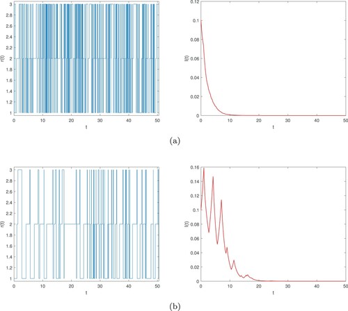
Case 2. If the infectious disease dies out in both subsystems and persists in one subsystem, then it may remain randomly extinct in the whole system (2(2) $\frac{\mathrm{d}{I}_k\left(t\right)}{\mathrm{d}t}=-I_k\left(t\right)+{\lambda }_{r\left(t\right)}k[1-I_k(t\left)\right]\theta \left(t\right),$(2) ). In this case, we let $F_1\left(t\right)$, $F_2\left(t\right)$ and $F_3\left(t\right)$ are gamma distributions with parameters ${\alpha }_1=0.8,{\text{β}}_1=0.6$; ${\alpha }_2=1.1,{\text{β}}_2=0.8$; ${\alpha }_3=0.7,{\text{β}}_3=0.186$, then the mean sojourn times are $m_1=1.3333,m_2=1.375$, $m_3=3.7634$, respectively. Other parameters of system (2(2) $\frac{\mathrm{d}{I}_k\left(t\right)}{\mathrm{d}t}=-I_k\left(t\right)+{\lambda }_{r\left(t\right)}k[1-I_k(t\left)\right]\theta \left(t\right),$(2) ) are assumed to be ${\lambda }_1=0.2,{\lambda }_2=0.15,{\lambda }_3=0.15,{\pi }_1=0.4,{\pi }_2=0.3,{\pi }_3=0.3,$ then $R_1=1.8,R_2=0.6139,R_3=0.75$. Obviously, $(R_1-1){\pi }_1{m}_1+(R_2-1){\pi }_2{m}_2+(R_3-1){\pi }_3{m}_3=-0.0148<0.$ We can see the global infected density $I\left(t\right)$ will almost surely tend to zero (see Figure 1(b)).

Case 3. If the infectious disease dies out in both subsystems and persists in one subsystem, then it may also remain randomly persistent in time mean in the whole system (2(2) $\frac{\mathrm{d}{I}_k\left(t\right)}{\mathrm{d}t}=-I_k\left(t\right)+{\lambda }_{r\left(t\right)}k[1-I_k(t\left)\right]\theta \left(t\right),$(2) ). In this case, we let $F_1\left(t\right)$, $F_2\left(t\right)$ and $F_3\left(t\right)$ are gamma distributions with parameters ${\alpha }_1=1.0,{\text{β}}_1=0.6$; ${\alpha }_2=0.5,{\text{β}}_2=0.7$; ${\alpha }_3=0.5,{\text{β}}_3=0.186$, then the mean sojourn times are $m_1=1.6667,m_2=0.7143$, $m_3=2.6882$, respectively. Other parameters of system (2(2) $\frac{\mathrm{d}{I}_k\left(t\right)}{\mathrm{d}t}=-I_k\left(t\right)+{\lambda }_{r\left(t\right)}k[1-I_k(t\left)\right]\theta \left(t\right),$(2) ) are assumed to be ${\lambda }_1=0.3,{\lambda }_2=0.15,{\lambda }_3=0.1,{\pi }_1=0.6,{\pi }_2=0.3,{\pi }_3=0.1,$ then $R_1=2.7,R_2=0.6139,R_3=0.5$. Obviously, $(R_1-1){\pi }_1{m}_1+(R_2-1){\pi }_2{m}_2+(R_3-1){\pi }_3{m}_3=1.4829>0.$ By Theorem 3.3, for any given initial value $(I_0,r_0)\in (0,1)\times \mathbb{S}$, system (2(2) $\frac{\mathrm{d}{I}_k\left(t\right)}{\mathrm{d}t}=-I_k\left(t\right)+{\lambda }_{r\left(t\right)}k[1-I_k(t\left)\right]\theta \left(t\right),$(2) ) will be persistent in time mean (see Figure 2(a)).

Figure 2. Numerical simulation of semi-Markov chain $r\left(t\right)$ and its corresponding global infected density in time mean $\frac{1}{t}{\int }_0^{t}I\left(s\right)\mathrm{d}s$. Switching times of $r\left(t\right)$ obey the gamma distribution.

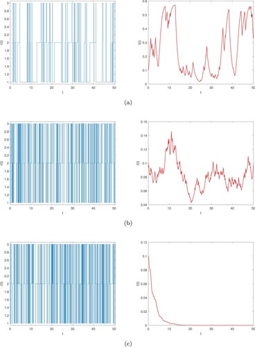
Case 4. If the infectious disease is persistent in all three subsystems, then it is still persistent in time mean in the whole system (2(2) $\frac{\mathrm{d}{I}_k\left(t\right)}{\mathrm{d}t}=-I_k\left(t\right)+{\lambda }_{r\left(t\right)}k[1-I_k(t\left)\right]\theta \left(t\right),$(2) ). In this case, we let $F_1\left(t\right)$, $F_2\left(t\right)$ and $F_3\left(t\right)$ are gamma distributions with parameters ${\alpha }_1=0.6,{\text{β}}_1=0.1389$; ${\alpha }_2=0.8,{\text{β}}_2=0.2148$; ${\alpha }_3=0.7,{\text{β}}_3=0.186$, then the mean sojourn times are $m_1=4.3197,m_2=3.7244$, $m_3=3.7634$, respectively. Other parameters of system (2(2) $\frac{\mathrm{d}{I}_k\left(t\right)}{\mathrm{d}t}=-I_k\left(t\right)+{\lambda }_{r\left(t\right)}k[1-I_k(t\left)\right]\theta \left(t\right),$(2) ) are assumed to be ${\lambda }_1=0.2,{\lambda }_2=0.4,{\lambda }_3=0.3,{\pi }_1=0.4,{\pi }_2=0.3,{\pi }_3=0.3,$ then $R_1=1.8,R_2=1.6372,R_3=1.5$. Obviously, $(R_1-1){\pi }_1{m}_1+(R_2-1){\pi }_2{m}_2+(R_3-1){\pi }_3{m}_3=2.6588>0.$ By Theorem 3.3, for any given initial value $(I_0,r_0)\in (0,1)\times \mathbb{S}$, epidemic will be persistent in time mean. Figure 2(b) simulates this case.

Case 5. If the infectious disease dies out in both subsystems and persists in one subsystem, then it may also remain be nonpersistent in time mean (2(2) $\frac{\mathrm{d}{I}_k\left(t\right)}{\mathrm{d}t}=-I_k\left(t\right)+{\lambda }_{r\left(t\right)}k[1-I_k(t\left)\right]\theta \left(t\right),$(2) ). In this case, we let $F_1\left(t\right)$, $F_2\left(t\right)$ and $F_3\left(t\right)$ are gamma distributions with parameters ${\alpha }_1=0.6,{\text{β}}_1=0.1389$; ${\alpha }_2=0.4,{\text{β}}_2=0.2148$; ${\alpha }_3=0.7,{\text{β}}_3=0.1947$, then the mean sojourn times are $m_1=4.3197,m_2=1.8622$, $m_3=3.5953$, respectively. Other parameters of system (2(2) $\frac{\mathrm{d}{I}_k\left(t\right)}{\mathrm{d}t}=-I_k\left(t\right)+{\lambda }_{r\left(t\right)}k[1-I_k(t\left)\right]\theta \left(t\right),$(2) ) are assumed to be ${\lambda }_1=0.1,{\lambda }_2=0.15,{\lambda }_3=0.25,{\pi }_1=0.25,{\pi }_2=0.3,{\pi }_3=0.4,$ then $R_1=0.9,R_2=0.6139,R_3=1.25$. Obviously, $(R_1-1){\pi }_1{m}_1+(R_2-1){\pi }_2{m}_2+(R_3-1){\pi }_3{m}_3=\mathrm{0.0000.}$ By Theorem 3.3, epidemic will be nonpersistent in time mean (see Figure 2(c)).

5. Conclusions

In this paper, we have studied the propagation dynamics of the temporal networks with random regime switching. Making use of a static network epidemic SIS model and the semi-Markov regime switching mechanism, we establish model (2(2) $\frac{\mathrm{d}{I}_k\left(t\right)}{\mathrm{d}t}=-I_k\left(t\right)+{\lambda }_{r\left(t\right)}k[1-I_k(t\left)\right]\theta \left(t\right),$(2) ) and its corresponding transformation form (5(5) $\frac{\mathrm{d}\theta \left(t\right)}{\mathrm{d}t}=\theta \left(t\right)\left[R_r-1-{\lambda }_r{〈k〉}_r^{-1}\sum _{k_r=1}^{n_r}{k}_r^{2}p\left(k_r\right)I_k\left(t\right)\right],$(5) ). A feasible method for analysing the basic reproduction number and threshold dynamics was proposed. It is the position of ${\mathcal{R}}_0$ with respect to 1, which decides whether the epidemic is persistent in time mean or extinct in theories and simulations. For the special case where Markov regime switching of system (2.2) in [4], a generalized version in a semi-Markov regime switching has been studied.

Acknowledgments

This work is supported by the National Natural Science Foundation of China (61873154,11331009,11971279), Shanxi Key Laboratory (201705D111006), Shanxi Scientific and Technology Innovation Team (201805D131012-1).

Disclosure statement

No potential conflict of interest was reported by the author(s).

Additional information

Funding

This work is supported by the National Natural Science Foundation of China [61873154; 11971279; 11331009], Shanxi Key Laboratory [201705D111006], Shanxi Scientific and Technology Innovation Team [201805D131012-1].

Notes

1 Without causing confusion, t is omitted in r(t) below.

References

- N. Bacaër, M. Khaladi, On the basic reproduction number in a random environment, J. Math. Biol. 67(6) (2013), pp. 1729–1739.
- F. Brauer, Epidemic models with heterogeneous mixing and treatment, Bull. Math. Biol. 70(7) (2008), pp. 1869–1885.
- X. Cao and Z. Jin, N-intertwined SIS epidemic model with markovian switching, Stoc. Dyn. 19 (2018), pp. 1950031.
- X. Cao and Z. Jin, Epidemic threshold and ergodicity of an SIS model in switched networks, J. Math. Anal. Appl. 479(1) (2019), pp. 1182–1194.
- I.I. Gihman and A.V. Skorohod, The Theory of Stochastic Processes II, Springer-Verlag, New York, 1975.
- P. Holme and J. Saramäki, Temporal networks, Phys. Reports 519(3) (2012), pp. 97–125.
- W.O. Kermack and A.G. Mckendrick, A contribution to the mathematical theory of epidemics, Proc. Roy. Soc. London A 115 (1927), pp. 700–721.
- D. Li, S. Liu, and J. Cui, Threshold dynamics and ergodicity of an SIRS epidemic model with semi-markov switching, J. Differ. Equ. 266(7) (2019), pp. 3973–4017.
- K. Li, H. Zhang, X. Fu, Y. Ding, and M. Small, Epidemic threshold determined by the first moments of network with alternating degree distributions, Phys. A: Stat. Mech. Appl. 419 (2015), pp. 585–593.
- N. Masuda and P. Holme, Temporal Network Epidemiology, Springer Nature, Singapore, 2017.
- J.C. Miller, Epidemic size and probability in populations with heterogeneous infectivity and susceptibility, Phys. Rev. E Stat. Nonlinear Soft. Matter Phys. 76(1 Pt 1) (2007), pp. 010101.
- M.E. Newman, Spread of epidemic disease on networks, Phys. Rev. E Stat. Nonlinear Soft Matter Phys. 66(1 Pt 2) (2002), pp. 016128.
- M. Ogura and V.M. Preciado, Stability of spreading processes over time-varying large-scale networks, IEEE Trans. Netw. Sci. Eng. 3(1) (2016), pp. 44–57.
- R. Pastor-Satorras and A. Vespignani, Epidemic spreading in scale-free networks, Phys. Rev. Lett.86(14) (2001), pp. 3200.
- R. Pastor-Satorras and A. Vespignani, Epidemic dynamics in finite size scale-free networks, Phys. Rev. E 65(3) (2002), pp. 035108.
- B.A. Prakash, H. Tong, N. Valler, M. Faloutsos, and C. Faloutsos, Virus propagation on time-varying networks: Theory and immunization algorithms, Joint European Conference on Machine Learning and Knowledge Discovery in Databases, Springer, 2010, pp. 99–114.
- M.R. Sanatkar, W.N. White, B. Natarajan, C.M. Scoglio, and K.A. Garrett, Epidemic threshold of an SIS model in dynamic switching networks, IEEE Trans. Syst. Man Cybern. Syst. 46(3) (2016), pp. 345–355.
- L. Speidel, K. Klemm, V.M. Eguíluz, and N. Masuda, Temporal interactions facilitate endemicity in the susceptible-infected-susceptible epidemic model, New J. Phys. 18(7) (2016), pp. 073013.
- E. Valdano, L. Ferreri, C. Poletto, and V. Colizza, Analytical computation of the epidemic threshold on temporal networks, Phys. Rev. X 18(3) (2014), pp. 503–512.
- A. Vazquez, B. Rácz, A. Lukács, and A.L. Barabási, Impact of non-Poissonian activity patterns on spreading processes, Phys. Rev. Lett. 98(15) (2007), pp. 158702.
- E. Volz and L.A. Meyers, Epidemic thresholds in dynamic contact networks, J. Roy. Soc. Interface6(32) (2009), p. 233.
- L. Wang and G.-Z. Dai, Global stability of virus spreading in complex heterogeneous networks, SIAM J. Appl. Math. 68(5) (2008), pp. 1495–1502.
- X. Yu, S. Yuan, and T. Zhang, Persistence and ergodicity of a stochastic single species model with allee effect under regime switching, Commun. Nonlinear Sci. Numer. Simul. 59 (2018), pp. 359–374.