A continuous-time mathematical model and discrete approximations for the aggregation of β-Amyloid

Abstract

Alzheimer's disease is a degenerative disorder characterized by the loss of synapses and neurons from the brain, as well as the accumulation of amyloid-based neuritic plaques. While it remains a matter of contention whether β-amyloid causes the neurodegeneration, β-amyloid aggregation is associated with the disease progression. Therefore, gaining a clearer understanding of this aggregation may help to better understand the disease. We develop a continuous-time model for β-amyloid aggregation using concepts from chemical kinetics and population dynamics. We show the model conserves mass and establish conditions for the existence and stability of equilibria. We also develop two discrete-time approximations to the model that are dynamically consistent. We show numerically that the continuous-time model produces sigmoidal growth, while the discrete-time approximations may exhibit oscillatory dynamics. Finally, sensitivity analysis reveals that aggregate concentration is most sensitive to parameters involved in monomer production and nucleation, suggesting the need for good estimates of such parameters.

Keywords:

• β-Amyloid
• Alzheimer's disease
• neurodegenerative diseases
• aggregation
• nonstandard discretization schemes

2010 Mathematics Subject Classification:

• 92C45

1. Introduction

Amyloid-β (Aβ) is a peptide generated by the proteolytic cleavage of the amyloid precursor protein (APP) by the action of β- and γ-secretases [10,28]. Aβ deposits in senile and neuritic plaques and hyperphosphorylated tau proteins in neurofibrillary tangles (NFT) are extracellular and intracellular expressions, respectively, of the Alzheimer's disease (AD) neuropathological phenotype, together with selective neuronal loss in hippocampal and neocortical regions. The accumulation of Aβ plaque in the brain is considered as one of the primary (postmortem) diagnostic criterion of AD [29,58,68]. Aβ is a 39- to 43- residue proteolytic product of a parental amyloid precursor protein (APP) that localizes to the plasma membrane, trans-Golgi network, endoplasmic reticulum (ER) and endosomal, lysosomal and mitochondrial membranes [69]. It is produced in the brain throughout life and it accumulates in the cerebral cortex in the elderly and to an excessive degree in AD, but its role in the etiology of Alzheimer's is unproven [60].

When Aβ is initially cleaved, it forms single pieces or monomers. The monomers are then thought to combine into clusters to form Aβ oligomers, and finally the oligomers form insoluble fibrils. This process is collectively known as aggregation. These fibrils further accumulate and become deposited as plaques. It is not clear how long this entire process takes, but some researchers hypothesize that it occurs over many years. Aβ can be produced by numerous types of cells such as neurons, astrocytes, neuroblastoma cells, hepatoma cells, fibroblasts and platelets, suggesting, along with its conserved sequence among different species, that this peptide should have an important function in normal cell development and maintenance [48].

One theory stipulates that the neurodegenerative effects of AD arise from Aβ. This is commonly known as the amyloid hypothesis and is one of the main models of AD pathogenesis [8,30,31,69,71,72]. For the case of Aβ linkage to AD, it has been found that Aβ becomes toxic once aggregated [32,64,70,74,78]. Moreover, numerous studies show a strong correlation between soluble Aβ oligomer levels and the extent of synaptic loss [13,14,24,28,41,46], further suggesting that the soluble oligomers are the causative agents of AD [47,49,76,77].

Despite mounting support from biochemical, genetic and transgenic animal studies in favour of the amyloid hypothesis, the hypothesis itself remains controversial [27,35,36,54,79]. Counter arguments to the amyloid hypothesis have been presented by many researchers. One of the central challenges is the fact that multiple clinical trials of anti-Aβ drugs have failed to reduce the symptoms of AD [40]. In fact, various immunotherapies targeting Aβ in AD model mice were effective in decreasing Aβ deposition in the brain, but it did not lead to the improvement of actual symptoms [57]. A more profound challenge to the amyloid hypothesis was put forth by Hyong-gon Lee et al. [38]. The authors suggest that Aβ, far from being the harbinger of disease, actually occurs secondary to more fundamental pathological changes and may even play a protective role in the diseased brain. Other researchers have put forward the hypothesis that the main factor underlying the progression of AD is the aggregation of tau protein and not Aβ [39].

Whether Aβ is the causal factor of AD or a downstream response to some as yet unidentified causative agent, the association of Aβ aggregation with AD means that understanding this process is of considerable importance. Consequently, in this paper we focus on modelling the process of Aβ aggregation. In its simplest forms, Aβ plaque formation can be described by protein aggregation, involving the misfolding of Aβ into soluble and insoluble assemblies [43,80]. Kinetic studies have suggested that the misfolding of monomeric Aβ has been shown to precede the formation of oligomers, which then serve as seeds for accelerated fibril growth [61], as illustrated in Figure 1. The two phases of Aβ aggregation are: (i) the nucleation phase, in which monomers undergo misfolding and associate to form oligomeric nuclei, and (ii) the elongation phase, in which the oligomeric nuclei rapidly grow by further addition of monomers, resulting in the formation of larger fibrils. The nucleation phase occurs gradually and at a slower rate than the elongation phase which proceeds it since elongation is more thermodynamically favourable [43]. A sigmoidal curve can thus describe this process.

Figure 1. The two phases of Aβ aggregation: from monomers to fibrils, adapted from [43]. We can expect to see a lag phase during the nucleation process followed by a phase of rapid growth (green curve). The addition of more oligomers (seeds) speeds up the process and induces faster aggregate formation (blue curve). In contrast, the lack of oligomers introduces lag time and slows down the aggregation process (red curve).

Mathematical models of Aβ kinetics provide a clearer mechanistic understanding of amyloid fibril growth. A number of mathematical models, both purely theoretical and experimentally driven, have been developed to describe the aggregation of Aβ. These include kinetic (ODE) models that consider the concentration of monomers and fibrils of length j [16,42], more complicated Smoluchowski-type (PDE) systems that incorporate the transportation and diffusion of fibrils [5,11,15,23,25,33,66], models that consider the impact of (hypothetical) treatment strategies [18,19,53,65], systems models to consider the role of Aβ in inflammation and neuron death [67], as well more experimentally driven models for AD including [52,59,63]. Previously, the authors [20] developed a discrete-time model for the aggregation of Aβ from monomers to diamers$,\dots$ up to pre-oligomers. This model was developed under the assumptions that aggregation occurs due to the addition of monomers, the aggregation process is not reversible and oligomers are formed from exactly six monomers. Hence they studied a discrete-time model with five states, i.e. a five-dimensional nonlinear discrete dynamical system.

In this paper, we develop a more general model that extends the model developed in [20] in several ways. First, we incorporate oligomer and fibril stages into the model. These additional stages allow us to model the two phases in the aggregation process: the slow nucleation stage that results in the formation of oligomers and the faster elongation stage that converts oligomers into fibrils. We note that, unlike the traditional kinetic equations (also called nucleation–polymerization models) that only model fibrils of length j, the stage-structured approach used here allows us to distinguish between the oligomer and fibril stage. This approach was motivated by studies that have shown kinetic models may not be best suited to reproduce the aggregation observed in laboratory studies. For instance, it was demonstrated for tau aggregation that the kinetic equations underestimate average fibril length and are inadequate at capturing oligomer concentrations over time. Meanwhile, a model that accounts for the conversion of oligomers to fibrils via a reaction of first order in monomer concentration was shown to provide a better fit [73]. Relatively few models for Aβ aggregation include this distinction between the two stages. Exceptions include [20, 39] which considered more complicated Smoluchowski-type (PDE) systems. Second, since various estimates have been given for average oligomer size (such as 6 [26], 8 [34], 2 or more [51]), here we do not assume that oligomers are formed by exactly six monomers. Instead, we leave the model flexible by assuming that oligomers are made of at least n + 1 monomers. This results in a system of differential equations with n + 2 states. All together, these assumptions mean that the model is adaptable and may be modified for different types of experimental data.

The paper is organized as follows. In Section 2, we develop a continuous-time model for Aβ aggregation. This model includes n equations for monomers and intermediate aggregates up to size n (where we use size to mean the number of monomers contained in an aggregate), as well as two equations for the oligomer and fibril stages. In Section 3, we provide a detailed analysis of the existence and stability of the equilibria of this model. Our main tool for locating the eigenvalues of the Jacobian matrix of the system is Gershogrin's Theorem [22,62]. Finally, in Section 4, we provide some numerical simulations to further study the continuous-time model as well as two discrete-time approximations which preserve the local dynamics. A summary of our results is provided in the Conclusion section.

2. The construction of the continuous-time model

To model the aggregation process of Aβ, we choose to model the slower nucleation phase as size structured, that is we consider the concentration of monomers $M_1$, diamers (2 monomers) $M_2$, triamers (3 monomers) $M_3$, …, etc. Meanwhile, we model the oligomer and fibril states as average stages O and P, respectively. We assume that oligomers are made of at least n + 1 monomers, resulting in a system containing n + 2 stages: the monomer stage $M_1$, the intermediate aggregate stages $M_2,\dots M_n$, the oligomer stage O, and the fibril stage P. We assume that aggregation (both nucleation and elongation) occurs via monomer addition. For simplicity, we do not consider disassociation (i.e., monomer removal from aggregates) or fibril fragmentation. We note that disassociation, which occurs at a slower rate than aggregation mechanisms, is typically neglected in analysis of kinetic models [9,16]. Meanwhile, fragmentation was shown not to be a dominant mechanism for aggregate formation [17]. Given these assumptions, the possible types of reactions may be illustrated as $\begin{array}{rl}{M}_1+M_1=2M_1& \to M_2\\ M_1+M_2& \to M_3\\ M_1+M_3& \to M_4\\ ⋮& \\ M_1+M_{n-1}& \to M_n\\ (O_a-n)M_1+M_n& \to O\\ (P_a-O_a)M_1+O& \to P\end{array}$where $O_a$ and $P_a$ give the average oligomer and fibril size, respectively. The first equation describes the primary nucleation process where we have assumed that the number of monomers making up the smallest stable aggregate, typically denoted by $n_c$, is 2. The last two equations describe multi-step processes where we have assumed that there is a rate determining step that is slower than the others. This is the same formulation that is used in [73] to describe these reactions.

Since monomers are produced in the brain, we assume that its production process is represented by a saturating function $f\left(M_1\right)M_1$. Here we take $f\left(M_1\right)M_1=\delta M_1(1-\frac{M_1}{\gamma })$, which is the logistic differential equation first introduced by Verhulst [75], where δ is the growth rate of monomers and γ is the carrying capacity. This choice of function was motivated by the assumption that monomer concentration cannot grow unbounded. However, we note that the following results would also hold for a general nonlinearity $f\left(M_1\right)$ satisfying the conditions $f\left(0\right)=\delta >0$ and $f^{\prime }\left(M_1\right)<0$. We also assume that there is degradation/clearance of each stage, denoted by ${\mu }_i$. While we do not distinguish between degradation and clearance here, in general degradation occurs at a faster rate than clearance [29]. All together, these assumptions result in the following model: (1) $\begin{array}{rl}\frac{\mathrm{d}{M}_1\left(t\right)}{\mathrm{d}t}& =\delta M_1\left(t\right)\left(1-\frac{M_1\left(t\right)}{\gamma }\right)-2K_1{M}_1^2\left(t\right)-M_1\left(t\right)\sum _{i=2}^{n-1}{K}_i{M}_i\left(t\right),\\ & -(O_a-n)K_n{M}_1\left(t\right)M_n\left(t\right)-(P_a-O_a)K_O{M}_1\left(t\right)O\left(t\right)-{\mu }_1{M}_1\left(t\right),\\ \frac{\mathrm{d}{M}_2\left(t\right)}{\mathrm{d}t}& =K_1{M}_1^2\left(t\right)-K_2{M}_1\left(t\right)M_2\left(t\right)-{\mu }_2{M}_2\left(t\right),\\ & ⋮\\ \frac{\mathrm{d}{M}_n\left(t\right)}{\mathrm{d}t}& =K_{n-1}{M}_1\left(t\right)M_{n-1}\left(t\right)-K_n{M}_1\left(t\right)M_n\left(t\right)-{\mu }_n{M}_n\left(t\right),\\ \frac{\mathrm{d}O\left(t\right)}{\mathrm{d}t}& =K_n{M}_1\left(t\right)M_n\left(t\right)-K_O{M}_1\left(t\right)O\left(t\right)-{\mu }_{O}O\left(t\right),\\ \frac{\mathrm{d}P\left(t\right)}{\mathrm{d}t}& =K_O{M}_1\left(t\right)O\left(t\right)-{\mu }_{P}P\left(t\right).\end{array}$(1) The factors $(O_a-n)$ and $(P_a-O_a)$ in the monomer equation represent the average number of monomers that need to be added to an $M_n$ aggregate to form an oligomer and the average number of monomers that need to be added to an oligomer to form a fibril, respectively. These factors ensure that the law of conservation of mass of the system is satisfied. The law states that the mass of the chemical components before the reaction is equal to the mass of the components after the reaction, that is, no monomers are lost or created through the aggregation process, as demonstrated by Lemma 2.1.

Lemma 2.1

The following equality holds: (2) $\sum _{i=1}^{n}i\frac{\mathrm{d}{M}_i}{\mathrm{d}t}+O_a\frac{\mathrm{d}O}{\mathrm{d}t}+P_a\frac{\mathrm{d}P}{\mathrm{d}t}=\delta M_1\left(1-\frac{M_1}{\gamma }\right)-\sum _{i=1}^{n}i{\mu }_i{M}_i-O_a{\mu }_{O}O-P_a{\mu }_{P}P.$(2)

Proof.

In model (1(1) $\begin{array}{rl}\frac{\mathrm{d}{M}_1\left(t\right)}{\mathrm{d}t}& =\delta M_1\left(t\right)\left(1-\frac{M_1\left(t\right)}{\gamma }\right)-2K_1{M}_1^2\left(t\right)-M_1\left(t\right)\sum _{i=2}^{n-1}{K}_i{M}_i\left(t\right),\\ & -(O_a-n)K_n{M}_1\left(t\right)M_n\left(t\right)-(P_a-O_a)K_O{M}_1\left(t\right)O\left(t\right)-{\mu }_1{M}_1\left(t\right),\\ \frac{\mathrm{d}{M}_2\left(t\right)}{\mathrm{d}t}& =K_1{M}_1^2\left(t\right)-K_2{M}_1\left(t\right)M_2\left(t\right)-{\mu }_2{M}_2\left(t\right),\\ & ⋮\\ \frac{\mathrm{d}{M}_n\left(t\right)}{\mathrm{d}t}& =K_{n-1}{M}_1\left(t\right)M_{n-1}\left(t\right)-K_n{M}_1\left(t\right)M_n\left(t\right)-{\mu }_n{M}_n\left(t\right),\\ \frac{\mathrm{d}O\left(t\right)}{\mathrm{d}t}& =K_n{M}_1\left(t\right)M_n\left(t\right)-K_O{M}_1\left(t\right)O\left(t\right)-{\mu }_{O}O\left(t\right),\\ \frac{\mathrm{d}P\left(t\right)}{\mathrm{d}t}& =K_O{M}_1\left(t\right)O\left(t\right)-{\mu }_{P}P\left(t\right).\end{array}$(1) ) multiply equation i by i for $i=1,\dots ,n$, equation O by $O_a$ and equation P by $P_a$ and then add up all the equations to get (2(2) $\sum _{i=1}^{n}i\frac{\mathrm{d}{M}_i}{\mathrm{d}t}+O_a\frac{\mathrm{d}O}{\mathrm{d}t}+P_a\frac{\mathrm{d}P}{\mathrm{d}t}=\delta M_1\left(1-\frac{M_1}{\gamma }\right)-\sum _{i=1}^{n}i{\mu }_i{M}_i-O_a{\mu }_{O}O-P_a{\mu }_{P}P.$(2) ).

Note that the above lemma shows that if the source and sink terms are zero, that is $\delta =0$, ${\mu }_i=0$, $i=1,\dots ,n$, ${\mu }_O=0$ and ${\mu }_P=0$, then Equation (2(2) $\sum _{i=1}^{n}i\frac{\mathrm{d}{M}_i}{\mathrm{d}t}+O_a\frac{\mathrm{d}O}{\mathrm{d}t}+P_a\frac{\mathrm{d}P}{\mathrm{d}t}=\delta M_1\left(1-\frac{M_1}{\gamma }\right)-\sum _{i=1}^{n}i{\mu }_i{M}_i-O_a{\mu }_{O}O-P_a{\mu }_{P}P.$(2) ) reduces to: (3) $\sum _{i=1}^{n}i\frac{\mathrm{d}{M}_i}{\mathrm{d}t}+O_a\frac{\mathrm{d}O}{\mathrm{d}t}+P_a\frac{\mathrm{d}P}{\mathrm{d}t}=0,$(3) which implies that $\sum _{i=1}^{n}i{M}_i+O_{a}O+P_{a}P=C$, i.e. the total number of monomers in all the aggregates is constant in time.

3. Existence and stability of equilibria

We now study the existence and stability of the equilibria of model (1(1) $\begin{array}{rl}\frac{\mathrm{d}{M}_1\left(t\right)}{\mathrm{d}t}& =\delta M_1\left(t\right)\left(1-\frac{M_1\left(t\right)}{\gamma }\right)-2K_1{M}_1^2\left(t\right)-M_1\left(t\right)\sum _{i=2}^{n-1}{K}_i{M}_i\left(t\right),\\ & -(O_a-n)K_n{M}_1\left(t\right)M_n\left(t\right)-(P_a-O_a)K_O{M}_1\left(t\right)O\left(t\right)-{\mu }_1{M}_1\left(t\right),\\ \frac{\mathrm{d}{M}_2\left(t\right)}{\mathrm{d}t}& =K_1{M}_1^2\left(t\right)-K_2{M}_1\left(t\right)M_2\left(t\right)-{\mu }_2{M}_2\left(t\right),\\ & ⋮\\ \frac{\mathrm{d}{M}_n\left(t\right)}{\mathrm{d}t}& =K_{n-1}{M}_1\left(t\right)M_{n-1}\left(t\right)-K_n{M}_1\left(t\right)M_n\left(t\right)-{\mu }_n{M}_n\left(t\right),\\ \frac{\mathrm{d}O\left(t\right)}{\mathrm{d}t}& =K_n{M}_1\left(t\right)M_n\left(t\right)-K_O{M}_1\left(t\right)O\left(t\right)-{\mu }_{O}O\left(t\right),\\ \frac{\mathrm{d}P\left(t\right)}{\mathrm{d}t}& =K_O{M}_1\left(t\right)O\left(t\right)-{\mu }_{P}P\left(t\right).\end{array}$(1) ). This model contains an extinction equilibrium and a unique positive equilibrium, as shown in Theorem 3.1.

Theorem 3.1

Consider model (1(1) $\begin{array}{rl}\frac{\mathrm{d}{M}_1\left(t\right)}{\mathrm{d}t}& =\delta M_1\left(t\right)\left(1-\frac{M_1\left(t\right)}{\gamma }\right)-2K_1{M}_1^2\left(t\right)-M_1\left(t\right)\sum _{i=2}^{n-1}{K}_i{M}_i\left(t\right),\\ & -(O_a-n)K_n{M}_1\left(t\right)M_n\left(t\right)-(P_a-O_a)K_O{M}_1\left(t\right)O\left(t\right)-{\mu }_1{M}_1\left(t\right),\\ \frac{\mathrm{d}{M}_2\left(t\right)}{\mathrm{d}t}& =K_1{M}_1^2\left(t\right)-K_2{M}_1\left(t\right)M_2\left(t\right)-{\mu }_2{M}_2\left(t\right),\\ & ⋮\\ \frac{\mathrm{d}{M}_n\left(t\right)}{\mathrm{d}t}& =K_{n-1}{M}_1\left(t\right)M_{n-1}\left(t\right)-K_n{M}_1\left(t\right)M_n\left(t\right)-{\mu }_n{M}_n\left(t\right),\\ \frac{\mathrm{d}O\left(t\right)}{\mathrm{d}t}& =K_n{M}_1\left(t\right)M_n\left(t\right)-K_O{M}_1\left(t\right)O\left(t\right)-{\mu }_{O}O\left(t\right),\\ \frac{\mathrm{d}P\left(t\right)}{\mathrm{d}t}& =K_O{M}_1\left(t\right)O\left(t\right)-{\mu }_{P}P\left(t\right).\end{array}$(1) ).

(i)

If $\delta -{\mu }_1\le 0$, then this system has only the extinction equilibrium $E^{\ast }=(0,0,\dots ,0)$.

(ii)

If $\delta -{\mu }_1>0$, then model (1(1) $\begin{array}{rl}\frac{\mathrm{d}{M}_1\left(t\right)}{\mathrm{d}t}& =\delta M_1\left(t\right)\left(1-\frac{M_1\left(t\right)}{\gamma }\right)-2K_1{M}_1^2\left(t\right)-M_1\left(t\right)\sum _{i=2}^{n-1}{K}_i{M}_i\left(t\right),\\ & -(O_a-n)K_n{M}_1\left(t\right)M_n\left(t\right)-(P_a-O_a)K_O{M}_1\left(t\right)O\left(t\right)-{\mu }_1{M}_1\left(t\right),\\ \frac{\mathrm{d}{M}_2\left(t\right)}{\mathrm{d}t}& =K_1{M}_1^2\left(t\right)-K_2{M}_1\left(t\right)M_2\left(t\right)-{\mu }_2{M}_2\left(t\right),\\ & ⋮\\ \frac{\mathrm{d}{M}_n\left(t\right)}{\mathrm{d}t}& =K_{n-1}{M}_1\left(t\right)M_{n-1}\left(t\right)-K_n{M}_1\left(t\right)M_n\left(t\right)-{\mu }_n{M}_n\left(t\right),\\ \frac{\mathrm{d}O\left(t\right)}{\mathrm{d}t}& =K_n{M}_1\left(t\right)M_n\left(t\right)-K_O{M}_1\left(t\right)O\left(t\right)-{\mu }_{O}O\left(t\right),\\ \frac{\mathrm{d}P\left(t\right)}{\mathrm{d}t}& =K_O{M}_1\left(t\right)O\left(t\right)-{\mu }_{P}P\left(t\right).\end{array}$(1) ) has, in addition to the extinction equilibrium $E^{\ast }$, a unique interior equilibrium $M^{\ast }=(M_1^{\ast },\dots ,M_n^{\ast },O^{\ast },P^{\ast })$, with all coordinates being positive.

Proof

The fact that $E^{\ast }=(0,0,\dots ,0)$ is always an equilibrium of the system is clear. To prove (ii), we note first that any equilibrium must satisfy the following: (4) $\begin{array}{rl}& \delta M_1\left(1-\frac{M_1}{\gamma }\right)-2K_1{M}_1^2\left(t\right)-M_1\sum _{i=2}^{n-1}{K}_i{M}_i\\ & -(O_a-n)K_n{M}_1{M}_n-(P_a-O_a)K_O{M}_{1}O-{\mu }_1{M}_1=0,\\ & K_1{M}_1^2-K_2{M}_1{M}_2-{\mu }_2{M}_2=0,\\ & ⋮\\ & K_{n-1}{M}_1{M}_{n-1}-K_n{M}_1{M}_n-{\mu }_n{M}_n=0,\\ & K_n{M}_1{M}_n-K_O{M}_1\left(t\right)O-{\mu }_{O}O=0,\\ & K_O{M}_1\left(t\right)O-{\mu }_{P}P=0.\end{array}$(4) From (4(4) $\begin{array}{rl}& \delta M_1\left(1-\frac{M_1}{\gamma }\right)-2K_1{M}_1^2\left(t\right)-M_1\sum _{i=2}^{n-1}{K}_i{M}_i\\ & -(O_a-n)K_n{M}_1{M}_n-(P_a-O_a)K_O{M}_{1}O-{\mu }_1{M}_1=0,\\ & K_1{M}_1^2-K_2{M}_1{M}_2-{\mu }_2{M}_2=0,\\ & ⋮\\ & K_{n-1}{M}_1{M}_{n-1}-K_n{M}_1{M}_n-{\mu }_n{M}_n=0,\\ & K_n{M}_1{M}_n-K_O{M}_1\left(t\right)O-{\mu }_{O}O=0,\\ & K_O{M}_1\left(t\right)O-{\mu }_{P}P=0.\end{array}$(4) ) we find that the coordinates $M_2,\dots ,M_n$, O and P for any equilibrium point must satisfy: (5) $\begin{array}{rl}{M}_i& =\frac{K_{i-1}{M}_1{M}_{i-1}}{K_i{M}_1+{\mu }_i}=\frac{K_1\dots K_{i-1}{M}_1^i}{{\mathrm{\Pi }}_{j=2}^i(K_j{M}_1+{\mu }_j)},i=2,\dots ,n,\end{array}$(5) (6) $\begin{array}{rl}O& =\frac{K_1\dots K_n{M}_1^{n+1}}{(K_O{M}_1+{\mu }_O){\mathrm{\Pi }}_{j=2}^n(K_j{M}_1+{\mu }_j)},\end{array}$(6) (7) $\begin{array}{rl}P& =\frac{K_O}{{\mu }_P}\frac{K_1\dots K_n{M}_1^{n+2}}{(K_O{M}_1+{\mu }_O){\mathrm{\Pi }}_{j=2}^n(K_j{M}_1+{\mu }_j)}.\end{array}$(7) From these equations it is easy to verify that $\frac{\mathrm{d}{M}_i}{\mathrm{d}{M}_1}>0$, for $i=2,\dots ,n$, $\frac{\mathrm{d}O}{\mathrm{d}{M}_1}>0$ and $\frac{\mathrm{d}P}{\mathrm{d}{M}_1}>0$. Now, to show $M_1$ has a positive fixed point coordinate, we divide the first equation of (4(4) $\begin{array}{rl}& \delta M_1\left(1-\frac{M_1}{\gamma }\right)-2K_1{M}_1^2\left(t\right)-M_1\sum _{i=2}^{n-1}{K}_i{M}_i\\ & -(O_a-n)K_n{M}_1{M}_n-(P_a-O_a)K_O{M}_{1}O-{\mu }_1{M}_1=0,\\ & K_1{M}_1^2-K_2{M}_1{M}_2-{\mu }_2{M}_2=0,\\ & ⋮\\ & K_{n-1}{M}_1{M}_{n-1}-K_n{M}_1{M}_n-{\mu }_n{M}_n=0,\\ & K_n{M}_1{M}_n-K_O{M}_1\left(t\right)O-{\mu }_{O}O=0,\\ & K_O{M}_1\left(t\right)O-{\mu }_{P}P=0.\end{array}$(4) ) by $M_1$ to obtain (8) $\begin{array}{rl}G\left(M_1\right)& :=\delta \left(1-\frac{M_1}{\gamma }\right)-2K_1{M}_1-\sum _{i=2}^{n-1}{K}_i{M}_i-(O_a-n)K_n{M}_n\\ & -(P_a-O_a)K_{O}O-{\mu }_1=0.\end{array}$(8) Clearly, $G\left(0\right)=\delta -{\mu }_1>0$. Furthermore, $\begin{array}{rl}\frac{\mathrm{d}G}{\mathrm{d}{M}_1}& =-\frac{\delta }{\gamma }-2K_1-\sum _{i=2}^{n-1}{K}_i\frac{\mathrm{d}{M}_i}{\mathrm{d}{M}_1}-(O_a-n)K_n\frac{\mathrm{d}{M}_n}{\mathrm{d}{M}_1}-(P_a-O_a)K_O\frac{\mathrm{d}O}{\mathrm{d}{M}_1}\\ & \le -\frac{\delta }{\gamma }-2K_1<0.\end{array}$Thus, G is a strictly decreasing function with $G\left(M_1\right)\to -\mathrm{\infty }$ as $M_1\to \mathrm{\infty }$. Hence, there exists a unique $M_1^{\ast }$ such $G\left(M_1^{\ast }\right)=0$. Plugging this $M_1^{\ast }$ into Equations (5(5) $\begin{array}{rl}{M}_i& =\frac{K_{i-1}{M}_1{M}_{i-1}}{K_i{M}_1+{\mu }_i}=\frac{K_1\dots K_{i-1}{M}_1^i}{{\mathrm{\Pi }}_{j=2}^i(K_j{M}_1+{\mu }_j)},i=2,\dots ,n,\end{array}$(5) )–(7(7) $\begin{array}{rl}P& =\frac{K_O}{{\mu }_P}\frac{K_1\dots K_n{M}_1^{n+2}}{(K_O{M}_1+{\mu }_O){\mathrm{\Pi }}_{j=2}^n(K_j{M}_1+{\mu }_j)}.\end{array}$(7) ) results in the unique positive equilibrium $M^{\ast }=(M_1^{\ast },\dots ,M_n^{\ast },O^{\ast },P^{\ast })$.

Next, we study the local stability of the two equilibria of the model, $E^{\ast }$ and $M^{\ast }$. The Jacobian matrix of (1(1) $\begin{array}{rl}\frac{\mathrm{d}{M}_1\left(t\right)}{\mathrm{d}t}& =\delta M_1\left(t\right)\left(1-\frac{M_1\left(t\right)}{\gamma }\right)-2K_1{M}_1^2\left(t\right)-M_1\left(t\right)\sum _{i=2}^{n-1}{K}_i{M}_i\left(t\right),\\ & -(O_a-n)K_n{M}_1\left(t\right)M_n\left(t\right)-(P_a-O_a)K_O{M}_1\left(t\right)O\left(t\right)-{\mu }_1{M}_1\left(t\right),\\ \frac{\mathrm{d}{M}_2\left(t\right)}{\mathrm{d}t}& =K_1{M}_1^2\left(t\right)-K_2{M}_1\left(t\right)M_2\left(t\right)-{\mu }_2{M}_2\left(t\right),\\ & ⋮\\ \frac{\mathrm{d}{M}_n\left(t\right)}{\mathrm{d}t}& =K_{n-1}{M}_1\left(t\right)M_{n-1}\left(t\right)-K_n{M}_1\left(t\right)M_n\left(t\right)-{\mu }_n{M}_n\left(t\right),\\ \frac{\mathrm{d}O\left(t\right)}{\mathrm{d}t}& =K_n{M}_1\left(t\right)M_n\left(t\right)-K_O{M}_1\left(t\right)O\left(t\right)-{\mu }_{O}O\left(t\right),\\ \frac{\mathrm{d}P\left(t\right)}{\mathrm{d}t}& =K_O{M}_1\left(t\right)O\left(t\right)-{\mu }_{P}P\left(t\right).\end{array}$(1) ) evaluated at $E^{\ast }$ is given by $J\left(E^{\ast }\right)=\left(\begin{array}{ccccccc}\delta -{\mu }_1& 0& 0& \cdots & 0& 0& 0\\ 0& -{\mu }_2& 0& \cdots & 0& 0& 0\\ 0& 0& -{\mu }_3& \cdots & 0& 0& 0\\ & & & \ddots & & & \\ 0& 0& 0& \cdots & -{\mu }_n& 0& 0\\ 0& 0& 0& 0& 0& -{\mu }_O& 0\\ 0& 0& 0& 0& 0& 0& -{\mu }_P\end{array}\right).$Clearly, the eigenvalues of $J\left(E^{\ast }\right)$ are given by ${\lambda }_1=\delta -{\mu }_1$, ${\lambda }_i=-{\mu }_i$, $i=2,\dots ,n$, ${\lambda }_{n+1}=-{\mu }_O$ and ${\lambda }_{n+2}=-{\mu }_P$. Therefore, $E^{\ast }$ is locally asymptotically stable if $\delta -\mu <0$ and unstable if $\delta -\mu >0$.

Next we compute the Jacobian matrix at the interior equilibrium $M^{\ast }$, $J\left(M^{\ast }\right)$, to obtain $\begin{array}{rl}& \left(\begin{array}{ccccc}-\frac{\delta }{\gamma }{M}_1^{\ast }-2K_1{M}_1^{\ast }& -K_2{M}_1^{\ast }& -K_3{M}_1^{\ast }& -K4M_1^{\ast }& \cdots \\ 2K_1{M}_1^{\ast }-K_2{M}_2^{\ast }& -K_2{M}_1^{\ast }-{\mu }_2& 0& 0& \cdots \\ K_2{M}_2^{\ast }-K_3{M}_3^{\ast }& K_2{M}_1^{\ast }& -K_3{M}_1^{\ast }-{\mu }_3& 0& \cdots \\ K_3{M}_3^{\ast }-K_4{M}_4^{\ast }& 0& K_3{M}_1^{\ast }& -K_4{M}_1^{\ast }-{\mu }_4& \cdots \\ & & & \ddots & \ddots \\ K_{n-1}{M}_{n-1}^{\ast }-K_n{M}_n^{\ast }& 0& \cdots & 0& 0\\ K_n{M}_n^{\ast }-K_O{O}^{\ast }& 0& \cdots & 0& 0\\ K_O{O}^{\ast }& 0& \cdots & 0& 0\end{array}\right.\\ & \left.\begin{array}{cccc}-K_{n-1}{M}_1^{\ast }& -(O_a-n)K_n{M}_1^{\ast }& -(P_a-O_a)K_O{M}_1^{\ast }& 0\\ 0& 0& 0& 0\\ 0& 0& 0\\ 0& 0& 0\\ & & & \\ K_{n-1}{M}_1^{\ast }& -K_n{M}_1^{\ast }-{\mu }_n& 0& 0\\ 0& K_n{M}_1^{\ast }& -K_o{M}_1^{\ast }-{\mu }_O& 0\\ 0& 0& K_O{M}_1^{\ast }& -{\mu }_P\end{array}\right).\end{array}$To determine the stability of $M^{\ast }$, we use the following result due to Gershgorin [62].

Theorem 3.2

Let $A=\left(a_{ij}\right)$ be a $k\times k$ matrix. Let $S_i$ be the disk in the complex plane with centre at $a_{ii}$, and radius $r_i=\sum _{j\ne i}^k\mid a_{ij}\mid$. Then all eigenvalues of A lie in $S={\cup }_{i=1}^k{S}_i$.

To this end, we assume that (9) $K_{i-1}<K_i$(9) and (10) $\sum _{i=2}^{n-1}{K}_i+(O_a-n)K_n+(P_a-O_a)K_O<\frac{\delta }{\gamma }+2K_1.$(10) Using (5(5) $\begin{array}{rl}{M}_i& =\frac{K_{i-1}{M}_1{M}_{i-1}}{K_i{M}_1+{\mu }_i}=\frac{K_1\dots K_{i-1}{M}_1^i}{{\mathrm{\Pi }}_{j=2}^i(K_j{M}_1+{\mu }_j)},i=2,\dots ,n,\end{array}$(5) )–(7(7) $\begin{array}{rl}P& =\frac{K_O}{{\mu }_P}\frac{K_1\dots K_n{M}_1^{n+2}}{(K_O{M}_1+{\mu }_O){\mathrm{\Pi }}_{j=2}^n(K_j{M}_1+{\mu }_j)}.\end{array}$(7) ) is easy to verify that (11) $K_1{M}_1^{\ast }>K_2{M}_2^{\ast }>\cdots >K_n{M}_n^{\ast }>K_O{O}^{\ast }.$(11) From this and assumption (9(9) $K_{i-1}<K_i$(9) ) if follows that (12) $M_1^{\ast }>M_2^{\ast }>\cdots >M_n^{\ast }>O^{\ast }.$(12) The following theorem summarizes the above stability analysis.

Theorem 3.3

Consider system (1(1) $\begin{array}{rl}\frac{\mathrm{d}{M}_1\left(t\right)}{\mathrm{d}t}& =\delta M_1\left(t\right)\left(1-\frac{M_1\left(t\right)}{\gamma }\right)-2K_1{M}_1^2\left(t\right)-M_1\left(t\right)\sum _{i=2}^{n-1}{K}_i{M}_i\left(t\right),\\ & -(O_a-n)K_n{M}_1\left(t\right)M_n\left(t\right)-(P_a-O_a)K_O{M}_1\left(t\right)O\left(t\right)-{\mu }_1{M}_1\left(t\right),\\ \frac{\mathrm{d}{M}_2\left(t\right)}{\mathrm{d}t}& =K_1{M}_1^2\left(t\right)-K_2{M}_1\left(t\right)M_2\left(t\right)-{\mu }_2{M}_2\left(t\right),\\ & ⋮\\ \frac{\mathrm{d}{M}_n\left(t\right)}{\mathrm{d}t}& =K_{n-1}{M}_1\left(t\right)M_{n-1}\left(t\right)-K_n{M}_1\left(t\right)M_n\left(t\right)-{\mu }_n{M}_n\left(t\right),\\ \frac{\mathrm{d}O\left(t\right)}{\mathrm{d}t}& =K_n{M}_1\left(t\right)M_n\left(t\right)-K_O{M}_1\left(t\right)O\left(t\right)-{\mu }_{O}O\left(t\right),\\ \frac{\mathrm{d}P\left(t\right)}{\mathrm{d}t}& =K_O{M}_1\left(t\right)O\left(t\right)-{\mu }_{P}P\left(t\right).\end{array}$(1) ).

(i)	$E^{\ast }$ is locally asymptotically stable if $\delta -{\mu }_1<0$ and unstable if $\delta -{\mu }_1>0$.
(ii)	If $\delta -{\mu }_1>0$ and conditions (9(9) $K_{i-1}<K_i$(9) )–(10(10) $\sum _{i=2}^{n-1}{K}_i+(O_a-n)K_n+(P_a-O_a)K_O<\frac{\delta }{\gamma }+2K_1.$(10) ) hold, then the unique positive equilibrium $M^{\ast }$ is locally asymptotically stable.

Proof.

Applying Theorem 3.2 we will show that all the Gerschgorin disks lie on the left-hand side of the complex plane, i.e., all eigenvalues have negative real part. To this end, consider the first Gershgorin disk $S_1$ centred at $a_{11}=-\frac{\delta }{\gamma }{M}_1^{\ast }-2K_1{M}_1^{\ast }$. Any eigenvalue that resides in $S_1$ must satisfy $|\lambda -a_{11}|=\left|\lambda +\frac{\delta }{\gamma }{M}_1^{\ast }+2K_1{M}_1^{\ast }\right|\le \sum _{i=2}^{n-1}{K}_i{M}_1^{\ast }+(O_a-n)K_n{M}_1^{\ast }+(P_a-O_a)K_O{M}_1^{\ast }.$From this we have the following two-sided inequality for the real part of λ, $\begin{array}{rl}& -\sum _{i=2}^{n-1}{K}_i{M}_1^{\ast }-(O_a-n)K_n{M}_1^{\ast }-(P_a-O_a)K_O{M}_1^{\ast }-\frac{\delta }{\gamma }{M}_1^{\ast }-2K_1{M}_1^{\ast }\le Re\lambda \\ & \le \sum _{i=2}^{n-1}{K}_i{M}_1^{\ast }+(O_a-n)K_n{M}_1^{\ast }+(P_a-O_a)K_O{M}_1^{\ast }-\frac{\delta }{\gamma }{M}_1^{\ast }-2K_1{M}_1^{\ast }.\end{array}$Simplifying we get: $\begin{array}{rl}& -M_1^{\ast }\left(\sum _{i=2}^{n-1}{K}_i+(O_a-n)K_n+(P_a-O_a)K_O+\frac{\delta }{\gamma }+2K_1\right)\le Re\lambda \\ & \le M_1^{\ast }\left(\sum _{i=2}^{n-1}{K}_i{M}_1^{\ast }+(O_a-n)K_n+(P_a-O_a)K_O-2K_1-\frac{\delta }{\gamma }\right)<0,\end{array}$by assumption (10(10) $\sum _{i=2}^{n-1}{K}_i+(O_a-n)K_n+(P_a-O_a)K_O<\frac{\delta }{\gamma }+2K_1.$(10) ). Thus such an eigenvalue must have a strictly negative real part.

Next, note that for $i=2,\dots ,n$ (13) $K_{i-1}{M}_{i-1}^{\ast }-K_i{M}_i^{\ast }=K_{i-1}{M}_{i-1}^{\ast }-K_{i-1}{M}_{i-1}^{\ast }\frac{K_i{M}_1^{\ast }}{K_i{M}_1^{\ast }+{\mu }_i}=K_{i-1}{M}_{i-1}^{\ast }\frac{{\mu }_i}{K_i{M}_1^{\ast }+{\mu }_i}>0.$(13) Consider the Gershgorin disk $S_i$, $i=2,\dots ,n$ centred at $a_{ii}=-K_i{M}_1^{\ast }-{\mu }_i$. Then we have $|\lambda -a_{ii}|=|\lambda +K_i{M}_1^{\ast }+{\mu }_i|\le K_{i-1}{M}_1^{\ast }+K_{i-1}{M}_{i-1}^{\ast }-K_i{M}_i^{\ast }.$Thus, $\begin{array}{rl}& -K_{i-1}{M}_1^{\ast }-(K_{i-1}{M}_{i-1}^{\ast }-K_i{M}_i^{\ast })-K_i{M}_1^{\ast }-{\mu }_i\\ & \le Re\lambda \le K_{i-1}{M}_1^{\ast }+K_{i-1}{M}_{i-1}^{\ast }-K_i{M}_i^{\ast }-K_i{M}_1^{\ast }-{\mu }_i.\end{array}$Applying assumption (9(9) $K_{i-1}<K_i$(9) ) and inequality (13(13) $K_{i-1}{M}_{i-1}^{\ast }-K_i{M}_i^{\ast }=K_{i-1}{M}_{i-1}^{\ast }-K_{i-1}{M}_{i-1}^{\ast }\frac{K_i{M}_1^{\ast }}{K_i{M}_1^{\ast }+{\mu }_i}=K_{i-1}{M}_{i-1}^{\ast }\frac{{\mu }_i}{K_i{M}_1^{\ast }+{\mu }_i}>0.$(13) ), we obtain $-K_{i-1}{M}_{i-1}^{\ast }\frac{{\mu }_i}{K_i{M}_1^{\ast }+{\mu }_i}-{\mu }_i\le Re\lambda \le K_{i-1}{M}_{i-1}^{\ast }\frac{{\mu }_i}{K_i{M}_1^{\ast }+{\mu }_i}-{\mu }_i.$From (9(9) $K_{i-1}<K_i$(9) ) and (10(10) $\sum _{i=2}^{n-1}{K}_i+(O_a-n)K_n+(P_a-O_a)K_O<\frac{\delta }{\gamma }+2K_1.$(10) ) it follows that $K_{i-1}{M}_{i-1}^{\ast }\frac{{\mu }_i}{K_i{M}_1^{\ast }+{\mu }_i}-{\mu }_i={\mu }_i\left(\frac{K_{i-1}{M}_{i-1}^{\ast }}{K_i{M}_1^{\ast }+{\mu }_i}-1\right)<{\mu }_i\left(\frac{K_i{M}_1^{\ast }}{K_i{M}_1^{\ast }+{\mu }_i}-1\right)<0.$Thus any eigenvalue in the disk $S_i$ must have a strictly negative real part. Similar arguments can be applied to $S_{n+1}$ and to $S_{n+2}$ centred at $a_{n+1,n+1}=-K_O{M}_1^{\ast }-{\mu }_O$ and at $a_{n+2,n+2}=-{\mu }_P$, respectively, to show that any eigenvalue in these two disks must have a negative real part. From the above it follows that all eigenvalues of the matrix which are in $S={\cup }_{i=1}^{n+2}{S}_i$ have negative real parts. Hence, $M^{\ast }$ is locally asymptotically stable.

Remark 3.4

One can also observe that $J\left(M^{\ast }\right)$ is a block matrix with two blocks: the first $(n+1)\times (n+1)$ elements and a $1\times 1$ block formed by the element $J_{n+2,n+2}$. Thus one of the eigenvalues is given by ${\lambda }_{n+1}=-{\mu }_P<0$ and hence it is sufficient to apply the above Gershgorin theorem to the block matrix obtained from the first $(n+1)\times (n+1)$ elements of $J\left(M^{\ast }\right)$ and show that the (remaining) n + 1 eigenvalues have negative real parts to obtain the conclusion of Theorem 3.3. The argument for showing that these eigenvalues have negative real parts is identical to that in the proof of Theorem 3.3.

Remark 3.5

The relation between the chemical reaction and the activation energy is governed by the Arrhenius equation [45]. The activation energy is the minimum energy needed for the reaction to occur, expressed in joules per mole. The Arrhenius equation states that the rate constant K of a chemical reaction depends primarily on the activation energy $E_a$ and temperature T: (14) $K=A{e}^{-\frac{E_a}{k_{B}T}},$(14) where the pre-exponential term A is related to the geometric and other secondary factors that may affect the frequency of collisions, and $k_B$ is the Boltzmann constant [45]. For near isothermal reactions, the primary factor is given by the activation energy. The accumulated electron cloud gets stronger as more monomers are added up. Therefore, the energy level of $M_{i+1}$ is lower than that of $M_i$, for $i=1,\dots ,n$, that is, $M_{i+1}$ is more stable than $M_i$. For this reason, the reverse reaction is ignored. We may conclude that $E_{a_1}>E_{a_2}>\cdots >E_{a_n}$. Given that the activation energy plays the primary role in determining the reaction rate constant, we obtain from the Arrhenius equation the relation: (15) $K_1<K_2<\cdots <K_n.$(15)

4. Numerical investigation

In this section, we use numerical simulations to further explore the dynamics of model (1(1) $\begin{array}{rl}\frac{\mathrm{d}{M}_1\left(t\right)}{\mathrm{d}t}& =\delta M_1\left(t\right)\left(1-\frac{M_1\left(t\right)}{\gamma }\right)-2K_1{M}_1^2\left(t\right)-M_1\left(t\right)\sum _{i=2}^{n-1}{K}_i{M}_i\left(t\right),\\ & -(O_a-n)K_n{M}_1\left(t\right)M_n\left(t\right)-(P_a-O_a)K_O{M}_1\left(t\right)O\left(t\right)-{\mu }_1{M}_1\left(t\right),\\ \frac{\mathrm{d}{M}_2\left(t\right)}{\mathrm{d}t}& =K_1{M}_1^2\left(t\right)-K_2{M}_1\left(t\right)M_2\left(t\right)-{\mu }_2{M}_2\left(t\right),\\ & ⋮\\ \frac{\mathrm{d}{M}_n\left(t\right)}{\mathrm{d}t}& =K_{n-1}{M}_1\left(t\right)M_{n-1}\left(t\right)-K_n{M}_1\left(t\right)M_n\left(t\right)-{\mu }_n{M}_n\left(t\right),\\ \frac{\mathrm{d}O\left(t\right)}{\mathrm{d}t}& =K_n{M}_1\left(t\right)M_n\left(t\right)-K_O{M}_1\left(t\right)O\left(t\right)-{\mu }_{O}O\left(t\right),\\ \frac{\mathrm{d}P\left(t\right)}{\mathrm{d}t}& =K_O{M}_1\left(t\right)O\left(t\right)-{\mu }_{P}P\left(t\right).\end{array}$(1) ) for parameter values lying outside of the region of stability predicted by Theorem 3.3. In addition, we also consider the dynamics of two discrete-time approximations of this model. Deriving discrete-time approximations to continuous-time aggregation models that preserve non-negativity, conservation of mass and the local dynamics of the continuous-time model is a challenging problem. In the appendix, we derive the two discrete-time models considered here and show that they preserve non-negativity and the local stability conditions for model (1(1) $\begin{array}{rl}\frac{\mathrm{d}{M}_1\left(t\right)}{\mathrm{d}t}& =\delta M_1\left(t\right)\left(1-\frac{M_1\left(t\right)}{\gamma }\right)-2K_1{M}_1^2\left(t\right)-M_1\left(t\right)\sum _{i=2}^{n-1}{K}_i{M}_i\left(t\right),\\ & -(O_a-n)K_n{M}_1\left(t\right)M_n\left(t\right)-(P_a-O_a)K_O{M}_1\left(t\right)O\left(t\right)-{\mu }_1{M}_1\left(t\right),\\ \frac{\mathrm{d}{M}_2\left(t\right)}{\mathrm{d}t}& =K_1{M}_1^2\left(t\right)-K_2{M}_1\left(t\right)M_2\left(t\right)-{\mu }_2{M}_2\left(t\right),\\ & ⋮\\ \frac{\mathrm{d}{M}_n\left(t\right)}{\mathrm{d}t}& =K_{n-1}{M}_1\left(t\right)M_{n-1}\left(t\right)-K_n{M}_1\left(t\right)M_n\left(t\right)-{\mu }_n{M}_n\left(t\right),\\ \frac{\mathrm{d}O\left(t\right)}{\mathrm{d}t}& =K_n{M}_1\left(t\right)M_n\left(t\right)-K_O{M}_1\left(t\right)O\left(t\right)-{\mu }_{O}O\left(t\right),\\ \frac{\mathrm{d}P\left(t\right)}{\mathrm{d}t}& =K_O{M}_1\left(t\right)O\left(t\right)-{\mu }_{P}P\left(t\right).\end{array}$(1) ). However, these models do not preserve the conservation of mass property of the continuous-time model and, as a result, we observe that they may produce cyclic dynamics when the continuous-time model produces stable equilibria. Importantly, we note that the model obtained using non-standard finite difference discretization (NFSD) is equivalent to the model developed in [20] with the additional modelling assumptions introduced in this paper. Therefore, the numerical simulations demonstrate that the continuous-time model is better able to describe the dynamics of Aβ aggregation than the previously developed model in [20].

Here we use simulations to address two questions. First, since the stability conditions obtained in Theorem 3.3(ii) are not sharp, what type of dynamics occur when these conditions are not met? Do we still have stable equilibria or are more complicated dynamics possible? Second, how do the solutions to the two discrete-time approximations compare to the solution to the continuous-time model? We showed in Theorems A.3 and A.4 that the discrete-time models preserve the local dynamics. This indicates that these solutions should agree well when conditions (9(9) $K_{i-1}<K_i$(9) )–(10(10) $\sum _{i=2}^{n-1}{K}_i+(O_a-n)K_n+(P_a-O_a)K_O<\frac{\delta }{\gamma }+2K_1.$(10) ) are met. However, these solutions are not guaranteed to agree for parameter values falling outside of the region defined by these conditions.

Biologically, the parameters involved in modelling the aggregation process of Aβ may have very different order of magnitude ranges. For instance, the nucleation rate may be as slow as ${10}^{-6}$M${}^{-1}$s${}^{-1}$ while the elongation rate may be as fast as ${10}^4$M${}^{-1}$s${}^{-1}$ [17]. Given this variability, where available we obtained parameter estimates, given in Table 1, from which we based our numerical simulations. However, we caution that the values used in the numerical simulations are solely for illustrative purposes and may not accurately reflect the rate constants for Aβ associated with AD as some estimates, such as those in [17,42], apply to forms of Aβ with enhanced aggregation.

Table 1. Parameter estimates of model (1(1) $\begin{array}{rl}\frac{\mathrm{d}{M}_1\left(t\right)}{\mathrm{d}t}& =\delta M_1\left(t\right)\left(1-\frac{M_1\left(t\right)}{\gamma }\right)-2K_1{M}_1^2\left(t\right)-M_1\left(t\right)\sum _{i=2}^{n-1}{K}_i{M}_i\left(t\right),\\ & -(O_a-n)K_n{M}_1\left(t\right)M_n\left(t\right)-(P_a-O_a)K_O{M}_1\left(t\right)O\left(t\right)-{\mu }_1{M}_1\left(t\right),\\ \frac{\mathrm{d}{M}_2\left(t\right)}{\mathrm{d}t}& =K_1{M}_1^2\left(t\right)-K_2{M}_1\left(t\right)M_2\left(t\right)-{\mu }_2{M}_2\left(t\right),\\ & ⋮\\ \frac{\mathrm{d}{M}_n\left(t\right)}{\mathrm{d}t}& =K_{n-1}{M}_1\left(t\right)M_{n-1}\left(t\right)-K_n{M}_1\left(t\right)M_n\left(t\right)-{\mu }_n{M}_n\left(t\right),\\ \frac{\mathrm{d}O\left(t\right)}{\mathrm{d}t}& =K_n{M}_1\left(t\right)M_n\left(t\right)-K_O{M}_1\left(t\right)O\left(t\right)-{\mu }_{O}O\left(t\right),\\ \frac{\mathrm{d}P\left(t\right)}{\mathrm{d}t}& =K_O{M}_1\left(t\right)O\left(t\right)-{\mu }_{P}P\left(t\right).\end{array}$(1) ) based on the literature.

Parameter	Meaning	Estimate	Reference
$K_1$	Nucleation rate	${10}^{-6}-{10}^{-4}$M${}^{-1}$s${}^{-1}$	[17,42]
$K_O$	Elongation rate	${10}^{-1}-{10}^4$M${}^{-1}$s${}^{-1}$	[17,19,42,52]
$O_a$	Average oligomer size	2−10	[26,34,51]
$P_a$	Average fibril size	$10-{10}^3$	[52]
${\mu }_1$	Degradation/clearance rate of monomers	${10}^{-5}-{10}^{-3}$s${}^{-1}$	[19,29]
${\mu }_O$	Degradation/clearance rate of oligomers	${10}^{-6}-{10}^{-4}$s${}^{-1}$	[29]
${\mu }_P$	Degradation/clearance rate of fibrils	${10}^{-7}-{10}^{-5}$s${}^{-1}$	Estimated

The estimates for the elongation rate given in Table 1 are based on the addition of a single monomer. Since the elongation rate $K_O$ in this model involves the addition of $P_a-O_a$ monomers, we modified this estimate based on the relative sizes of the fibril and oligomer stages. In [29], the authors estimated the degradation rate of oligomers as $1/10{\mu }_1$. Therefore, to estimate the degradation rate of fibrils, we assume, based on relative sizes, that ${\mu }_P=1/10{\mu }_O=1/100{\mu }_1$. Since we may expect the degradation rates of aggregates to decrease with aggregate size, while the nucleation rates increase with aggregate size (see Remark 3.5), to pick values of ${\mu }_i$ and $K_i$, for $2\le i\le n$, we choose relationships that satisfy these. Specifically, we use the relations (16) ${\mu }_i={\mu }_1/i,K_i=K_{i-1}+ϵ,1\le i\le n,\mathrm{f}\mathrm{o}\mathrm{r}\mathrm{s}\mathrm{o}\mathrm{m}\mathrm{e}\mathrm{c}\mathrm{o}\mathrm{n}\mathrm{s}\mathrm{t}\mathrm{a}\mathrm{n}\mathrm{t}ϵ>0.$(16) Notice that with this choice of $K_i$, condition (9(9) $K_{i-1}<K_i$(9) ) is always satisfied. We were unable to obtain estimates for the production rate of monomers δ or the carrying capacity of monomers γ. Therefore, in our simulations, we choose an arbitrary value of δ that makes the extinction equilibrium unstable, $\delta -{\mu }_1>0$, and vary the value of γ to change the value of (17) $D:=\sum _{i=2}^{n-1}{K}_i+(O_a-n)K_n+(P_a-O_a)K_O-\frac{\delta }{\gamma }-2K_1,$(17) which gives a locally asymptotically stable positive equilibrium when this quantity is negative (see condition (10(10) $\sum _{i=2}^{n-1}{K}_i+(O_a-n)K_n+(P_a-O_a)K_O<\frac{\delta }{\gamma }+2K_1.$(10) )).

In the simulations presented in Figures 2–5, we use the parameter values (18) $\begin{array}{rl}& \delta =50,K_1={10}^{-4},K_O=0.1,n=6,O_a=10,P_a=100,\\ & {\mu }_1={10}^{-3},{\mu }_O={10}^{-4},{\mu }_P={10}^{-5},ϵ=0.001,\end{array}$(18) together with the relationships given in (16(16) ${\mu }_i={\mu }_1/i,K_i=K_{i-1}+ϵ,1\le i\le n,\mathrm{f}\mathrm{o}\mathrm{r}\mathrm{s}\mathrm{o}\mathrm{m}\mathrm{e}\mathrm{c}\mathrm{o}\mathrm{n}\mathrm{s}\mathrm{t}\mathrm{a}\mathrm{n}\mathrm{t}ϵ>0.$(16) ) and the initial condition $M_1=10$, $M_2=\cdots M_6=O=P=0$. In Figure 2(a), we show the time series dynamics for models (1(1) $\begin{array}{rl}\frac{\mathrm{d}{M}_1\left(t\right)}{\mathrm{d}t}& =\delta M_1\left(t\right)\left(1-\frac{M_1\left(t\right)}{\gamma }\right)-2K_1{M}_1^2\left(t\right)-M_1\left(t\right)\sum _{i=2}^{n-1}{K}_i{M}_i\left(t\right),\\ & -(O_a-n)K_n{M}_1\left(t\right)M_n\left(t\right)-(P_a-O_a)K_O{M}_1\left(t\right)O\left(t\right)-{\mu }_1{M}_1\left(t\right),\\ \frac{\mathrm{d}{M}_2\left(t\right)}{\mathrm{d}t}& =K_1{M}_1^2\left(t\right)-K_2{M}_1\left(t\right)M_2\left(t\right)-{\mu }_2{M}_2\left(t\right),\\ & ⋮\\ \frac{\mathrm{d}{M}_n\left(t\right)}{\mathrm{d}t}& =K_{n-1}{M}_1\left(t\right)M_{n-1}\left(t\right)-K_n{M}_1\left(t\right)M_n\left(t\right)-{\mu }_n{M}_n\left(t\right),\\ \frac{\mathrm{d}O\left(t\right)}{\mathrm{d}t}& =K_n{M}_1\left(t\right)M_n\left(t\right)-K_O{M}_1\left(t\right)O\left(t\right)-{\mu }_{O}O\left(t\right),\\ \frac{\mathrm{d}P\left(t\right)}{\mathrm{d}t}& =K_O{M}_1\left(t\right)O\left(t\right)-{\mu }_{P}P\left(t\right).\end{array}$(1) ), (A1(A1) $\begin{array}{rl}{M}_1(t+1)& =(1+\delta )M_1\left(t\right)\left[1+{\mu }_1+\frac{\delta }{\gamma }{M}_1\left(t\right)+2K_1{M}_1\left(t\right)+\sum _{i=2}^{n-1}{K}_i{M}_i\left(t\right)\right.\\ & {\left.+(O_a-n)K_n{M}_n\left(t\right)+(P_a-O_a)K_{O}O\left(t\right)\phantom{\frac{1}{2}}\right]}^{-1},\\ M_2(t+1)& =\frac{M_2\left(t\right)+K_1{M}_1^2\left(t\right)}{1+{\mu }_2+K_2{M}_1\left(t\right)},\\ M_3(t+1)& =\frac{M_3\left(t\right)+K_2{M}_1\left(t\right)M_2\left(t\right)}{1+{\mu }_3+K_3{M}_1\left(t\right)},\\ & ⋮\\ M_n(t+1)& =\frac{M_n\left(t\right)+K_{n-1}{M}_1\left(t\right)M_{n-1}\left(t\right)}{1+{\mu }_n+K_n{M}_1\left(t\right)},\\ O(t+1)& =\frac{O\left(t\right)+K_n{M}_1\left(t\right)M_n\left(t\right)}{1+{\mu }_O+K_O{M}_1\left(t\right)},\\ P(t+1)& =\frac{P\left(t\right)+K_O{M}_1\left(t\right)O\left(t\right)}{1+{\mu }_P}.\end{array}$(A1) ) and (A2(A2) $\begin{array}{rl}{M}_1(t+1)& =e^{(\delta -{\mu }_1)}{M}_1\left(t\right)\left[1+{\varphi }_1\left(1\right)\left(\frac{\delta }{\gamma }{M}_1\left(t\right)+2K_1{M}_1\left(t\right)+\sum _{i=2}^{n-1}{K}_i{M}_i\left(t\right)\right.\right.\\ & {\left.\left.+(O_a-n)K_n{M}_n\left(t\right)+(P_a-O_a)K_{O}O\left(t\right)\phantom{\frac{1}{2}}\right)\right]}^{-1},\\ M_2(t+1)& =\frac{e^{-{\mu }_2}{M}_2\left(t\right)+{\varphi }_2\left(1\right)K_1{M}_1^2\left(t\right)}{1+{\varphi }_2\left(1\right)K_2{M}_1\left(t\right))},\\ M_3(t+1)& =\frac{e^{-{\mu }_3}{M}_3\left(t\right)+{\varphi }_3\left(1\right)K_2{M}_1\left(t\right)M_2\left(t\right)}{1+{\varphi }_3\left(1\right)K_3{M}_1\left(t\right))},\\ & ⋮\\ M_n(t+1)& =\frac{e^{-{\mu }_n}{M}_n\left(t\right)+{\varphi }_n\left(1\right)K_{n-1}{M}_1\left(t\right)M_{n-1}\left(t\right)}{1+{\varphi }_n\left(1\right)K_n{M}_1\left(t\right))},\\ O(t+1)& =\frac{e^{-{\mu }_O}O\left(t\right)+{\varphi }_O\left(1\right)K_n{M}_1\left(t\right)M_n\left(t\right)}{1+{\varphi }_O\left(1\right)K_O{M}_1\left(t\right)},\\ P(t+1)& =e^{-{\mu }_P}P\left(t\right)+{\varphi }_P\left(1\right)K_O{M}_1\left(t\right)O\left(t\right).\end{array}$(A2) ) when $\gamma =75$ resulting in D = 8.3639>0. This first figure demonstrates that the region of stability for the positive equilibrium extends beyond the stability region established in Theorem 3.3, as determined by condition (10(10) $\sum _{i=2}^{n-1}{K}_i+(O_a-n)K_n+(P_a-O_a)K_O<\frac{\delta }{\gamma }+2K_1.$(10) ). The transience for all three models follows a sigmoidal curve and, as is to be expected, the larger aggregates take longer to reach equilibrium, with the fibril stage taking much longer than the others. In Figure 2(b), we show the time-series dynamics when γ is increased to $\gamma =5000$ resulting in D = 9.0206. In this figure, we observe that all models still converge to a stable positive equilibrium. However, both discrete-time models exhibit transient oscillations. Increasing γ even further to $\gamma =8000$, resulting in D = 9.0244, we observe in Figure 3 that the discrete-time approximations no longer agree with the continuous-time model. Instead, model (1(1) $\begin{array}{rl}\frac{\mathrm{d}{M}_1\left(t\right)}{\mathrm{d}t}& =\delta M_1\left(t\right)\left(1-\frac{M_1\left(t\right)}{\gamma }\right)-2K_1{M}_1^2\left(t\right)-M_1\left(t\right)\sum _{i=2}^{n-1}{K}_i{M}_i\left(t\right),\\ & -(O_a-n)K_n{M}_1\left(t\right)M_n\left(t\right)-(P_a-O_a)K_O{M}_1\left(t\right)O\left(t\right)-{\mu }_1{M}_1\left(t\right),\\ \frac{\mathrm{d}{M}_2\left(t\right)}{\mathrm{d}t}& =K_1{M}_1^2\left(t\right)-K_2{M}_1\left(t\right)M_2\left(t\right)-{\mu }_2{M}_2\left(t\right),\\ & ⋮\\ \frac{\mathrm{d}{M}_n\left(t\right)}{\mathrm{d}t}& =K_{n-1}{M}_1\left(t\right)M_{n-1}\left(t\right)-K_n{M}_1\left(t\right)M_n\left(t\right)-{\mu }_n{M}_n\left(t\right),\\ \frac{\mathrm{d}O\left(t\right)}{\mathrm{d}t}& =K_n{M}_1\left(t\right)M_n\left(t\right)-K_O{M}_1\left(t\right)O\left(t\right)-{\mu }_{O}O\left(t\right),\\ \frac{\mathrm{d}P\left(t\right)}{\mathrm{d}t}& =K_O{M}_1\left(t\right)O\left(t\right)-{\mu }_{P}P\left(t\right).\end{array}$(1) ) equilibrates while the two discrete-time models converge to stable cycles that oscillate around this equilibrium value.

Figure 2. The time series dynamics of the continuous-time model (1(1) $\begin{array}{rl}\frac{\mathrm{d}{M}_1\left(t\right)}{\mathrm{d}t}& =\delta M_1\left(t\right)\left(1-\frac{M_1\left(t\right)}{\gamma }\right)-2K_1{M}_1^2\left(t\right)-M_1\left(t\right)\sum _{i=2}^{n-1}{K}_i{M}_i\left(t\right),\\ & -(O_a-n)K_n{M}_1\left(t\right)M_n\left(t\right)-(P_a-O_a)K_O{M}_1\left(t\right)O\left(t\right)-{\mu }_1{M}_1\left(t\right),\\ \frac{\mathrm{d}{M}_2\left(t\right)}{\mathrm{d}t}& =K_1{M}_1^2\left(t\right)-K_2{M}_1\left(t\right)M_2\left(t\right)-{\mu }_2{M}_2\left(t\right),\\ & ⋮\\ \frac{\mathrm{d}{M}_n\left(t\right)}{\mathrm{d}t}& =K_{n-1}{M}_1\left(t\right)M_{n-1}\left(t\right)-K_n{M}_1\left(t\right)M_n\left(t\right)-{\mu }_n{M}_n\left(t\right),\\ \frac{\mathrm{d}O\left(t\right)}{\mathrm{d}t}& =K_n{M}_1\left(t\right)M_n\left(t\right)-K_O{M}_1\left(t\right)O\left(t\right)-{\mu }_{O}O\left(t\right),\\ \frac{\mathrm{d}P\left(t\right)}{\mathrm{d}t}& =K_O{M}_1\left(t\right)O\left(t\right)-{\mu }_{P}P\left(t\right).\end{array}$(1) ) (dotted blue line), and the discrete-time models (A1(A1) $\begin{array}{rl}{M}_1(t+1)& =(1+\delta )M_1\left(t\right)\left[1+{\mu }_1+\frac{\delta }{\gamma }{M}_1\left(t\right)+2K_1{M}_1\left(t\right)+\sum _{i=2}^{n-1}{K}_i{M}_i\left(t\right)\right.\\ & {\left.+(O_a-n)K_n{M}_n\left(t\right)+(P_a-O_a)K_{O}O\left(t\right)\phantom{\frac{1}{2}}\right]}^{-1},\\ M_2(t+1)& =\frac{M_2\left(t\right)+K_1{M}_1^2\left(t\right)}{1+{\mu }_2+K_2{M}_1\left(t\right)},\\ M_3(t+1)& =\frac{M_3\left(t\right)+K_2{M}_1\left(t\right)M_2\left(t\right)}{1+{\mu }_3+K_3{M}_1\left(t\right)},\\ & ⋮\\ M_n(t+1)& =\frac{M_n\left(t\right)+K_{n-1}{M}_1\left(t\right)M_{n-1}\left(t\right)}{1+{\mu }_n+K_n{M}_1\left(t\right)},\\ O(t+1)& =\frac{O\left(t\right)+K_n{M}_1\left(t\right)M_n\left(t\right)}{1+{\mu }_O+K_O{M}_1\left(t\right)},\\ P(t+1)& =\frac{P\left(t\right)+K_O{M}_1\left(t\right)O\left(t\right)}{1+{\mu }_P}.\end{array}$(A1) ) (solid red line) and (A2(A2) $\begin{array}{rl}{M}_1(t+1)& =e^{(\delta -{\mu }_1)}{M}_1\left(t\right)\left[1+{\varphi }_1\left(1\right)\left(\frac{\delta }{\gamma }{M}_1\left(t\right)+2K_1{M}_1\left(t\right)+\sum _{i=2}^{n-1}{K}_i{M}_i\left(t\right)\right.\right.\\ & {\left.\left.+(O_a-n)K_n{M}_n\left(t\right)+(P_a-O_a)K_{O}O\left(t\right)\phantom{\frac{1}{2}}\right)\right]}^{-1},\\ M_2(t+1)& =\frac{e^{-{\mu }_2}{M}_2\left(t\right)+{\varphi }_2\left(1\right)K_1{M}_1^2\left(t\right)}{1+{\varphi }_2\left(1\right)K_2{M}_1\left(t\right))},\\ M_3(t+1)& =\frac{e^{-{\mu }_3}{M}_3\left(t\right)+{\varphi }_3\left(1\right)K_2{M}_1\left(t\right)M_2\left(t\right)}{1+{\varphi }_3\left(1\right)K_3{M}_1\left(t\right))},\\ & ⋮\\ M_n(t+1)& =\frac{e^{-{\mu }_n}{M}_n\left(t\right)+{\varphi }_n\left(1\right)K_{n-1}{M}_1\left(t\right)M_{n-1}\left(t\right)}{1+{\varphi }_n\left(1\right)K_n{M}_1\left(t\right))},\\ O(t+1)& =\frac{e^{-{\mu }_O}O\left(t\right)+{\varphi }_O\left(1\right)K_n{M}_1\left(t\right)M_n\left(t\right)}{1+{\varphi }_O\left(1\right)K_O{M}_1\left(t\right)},\\ P(t+1)& =e^{-{\mu }_P}P\left(t\right)+{\varphi }_P\left(1\right)K_O{M}_1\left(t\right)O\left(t\right).\end{array}$(A2) ) (dashed yellow line) for (a) $\gamma =75$ and (b) $\gamma =5000$, and all other parameters given by (18(18) $\begin{array}{rl}& \delta =50,K_1={10}^{-4},K_O=0.1,n=6,O_a=10,P_a=100,\\ & {\mu }_1={10}^{-3},{\mu }_O={10}^{-4},{\mu }_P={10}^{-5},ϵ=0.001,\end{array}$(18) ) and (16(16) ${\mu }_i={\mu }_1/i,K_i=K_{i-1}+ϵ,1\le i\le n,\mathrm{f}\mathrm{o}\mathrm{r}\mathrm{s}\mathrm{o}\mathrm{m}\mathrm{e}\mathrm{c}\mathrm{o}\mathrm{n}\mathrm{s}\mathrm{t}\mathrm{a}\mathrm{n}\mathrm{t}ϵ>0.$(16) ).

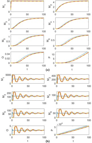
Figure 3. The time series dynamics of the continuous-time model (1(1) $\begin{array}{rl}\frac{\mathrm{d}{M}_1\left(t\right)}{\mathrm{d}t}& =\delta M_1\left(t\right)\left(1-\frac{M_1\left(t\right)}{\gamma }\right)-2K_1{M}_1^2\left(t\right)-M_1\left(t\right)\sum _{i=2}^{n-1}{K}_i{M}_i\left(t\right),\\ & -(O_a-n)K_n{M}_1\left(t\right)M_n\left(t\right)-(P_a-O_a)K_O{M}_1\left(t\right)O\left(t\right)-{\mu }_1{M}_1\left(t\right),\\ \frac{\mathrm{d}{M}_2\left(t\right)}{\mathrm{d}t}& =K_1{M}_1^2\left(t\right)-K_2{M}_1\left(t\right)M_2\left(t\right)-{\mu }_2{M}_2\left(t\right),\\ & ⋮\\ \frac{\mathrm{d}{M}_n\left(t\right)}{\mathrm{d}t}& =K_{n-1}{M}_1\left(t\right)M_{n-1}\left(t\right)-K_n{M}_1\left(t\right)M_n\left(t\right)-{\mu }_n{M}_n\left(t\right),\\ \frac{\mathrm{d}O\left(t\right)}{\mathrm{d}t}& =K_n{M}_1\left(t\right)M_n\left(t\right)-K_O{M}_1\left(t\right)O\left(t\right)-{\mu }_{O}O\left(t\right),\\ \frac{\mathrm{d}P\left(t\right)}{\mathrm{d}t}& =K_O{M}_1\left(t\right)O\left(t\right)-{\mu }_{P}P\left(t\right).\end{array}$(1) ) (dotted blue line), and the discrete-time models (A1(A1) $\begin{array}{rl}{M}_1(t+1)& =(1+\delta )M_1\left(t\right)\left[1+{\mu }_1+\frac{\delta }{\gamma }{M}_1\left(t\right)+2K_1{M}_1\left(t\right)+\sum _{i=2}^{n-1}{K}_i{M}_i\left(t\right)\right.\\ & {\left.+(O_a-n)K_n{M}_n\left(t\right)+(P_a-O_a)K_{O}O\left(t\right)\phantom{\frac{1}{2}}\right]}^{-1},\\ M_2(t+1)& =\frac{M_2\left(t\right)+K_1{M}_1^2\left(t\right)}{1+{\mu }_2+K_2{M}_1\left(t\right)},\\ M_3(t+1)& =\frac{M_3\left(t\right)+K_2{M}_1\left(t\right)M_2\left(t\right)}{1+{\mu }_3+K_3{M}_1\left(t\right)},\\ & ⋮\\ M_n(t+1)& =\frac{M_n\left(t\right)+K_{n-1}{M}_1\left(t\right)M_{n-1}\left(t\right)}{1+{\mu }_n+K_n{M}_1\left(t\right)},\\ O(t+1)& =\frac{O\left(t\right)+K_n{M}_1\left(t\right)M_n\left(t\right)}{1+{\mu }_O+K_O{M}_1\left(t\right)},\\ P(t+1)& =\frac{P\left(t\right)+K_O{M}_1\left(t\right)O\left(t\right)}{1+{\mu }_P}.\end{array}$(A1) ) (solid red line) and (A2(A2) $\begin{array}{rl}{M}_1(t+1)& =e^{(\delta -{\mu }_1)}{M}_1\left(t\right)\left[1+{\varphi }_1\left(1\right)\left(\frac{\delta }{\gamma }{M}_1\left(t\right)+2K_1{M}_1\left(t\right)+\sum _{i=2}^{n-1}{K}_i{M}_i\left(t\right)\right.\right.\\ & {\left.\left.+(O_a-n)K_n{M}_n\left(t\right)+(P_a-O_a)K_{O}O\left(t\right)\phantom{\frac{1}{2}}\right)\right]}^{-1},\\ M_2(t+1)& =\frac{e^{-{\mu }_2}{M}_2\left(t\right)+{\varphi }_2\left(1\right)K_1{M}_1^2\left(t\right)}{1+{\varphi }_2\left(1\right)K_2{M}_1\left(t\right))},\\ M_3(t+1)& =\frac{e^{-{\mu }_3}{M}_3\left(t\right)+{\varphi }_3\left(1\right)K_2{M}_1\left(t\right)M_2\left(t\right)}{1+{\varphi }_3\left(1\right)K_3{M}_1\left(t\right))},\\ & ⋮\\ M_n(t+1)& =\frac{e^{-{\mu }_n}{M}_n\left(t\right)+{\varphi }_n\left(1\right)K_{n-1}{M}_1\left(t\right)M_{n-1}\left(t\right)}{1+{\varphi }_n\left(1\right)K_n{M}_1\left(t\right))},\\ O(t+1)& =\frac{e^{-{\mu }_O}O\left(t\right)+{\varphi }_O\left(1\right)K_n{M}_1\left(t\right)M_n\left(t\right)}{1+{\varphi }_O\left(1\right)K_O{M}_1\left(t\right)},\\ P(t+1)& =e^{-{\mu }_P}P\left(t\right)+{\varphi }_P\left(1\right)K_O{M}_1\left(t\right)O\left(t\right).\end{array}$(A2) ) (dashed yellow line) for (a) $\gamma =8000$ and all other parameters given by (18(18) $\begin{array}{rl}& \delta =50,K_1={10}^{-4},K_O=0.1,n=6,O_a=10,P_a=100,\\ & {\mu }_1={10}^{-3},{\mu }_O={10}^{-4},{\mu }_P={10}^{-5},ϵ=0.001,\end{array}$(18) ) and (16(16) ${\mu }_i={\mu }_1/i,K_i=K_{i-1}+ϵ,1\le i\le n,\mathrm{f}\mathrm{o}\mathrm{r}\mathrm{s}\mathrm{o}\mathrm{m}\mathrm{e}\mathrm{c}\mathrm{o}\mathrm{n}\mathrm{s}\mathrm{t}\mathrm{a}\mathrm{n}\mathrm{t}ϵ>0.$(16) ) and (b) $\gamma =30,000$ and the other parameters the same as (a) except for $K_O=0.01$ and ${\mu }_1=\cdots ={\mu }_n={\mu }_O={\mu }_P=1$.

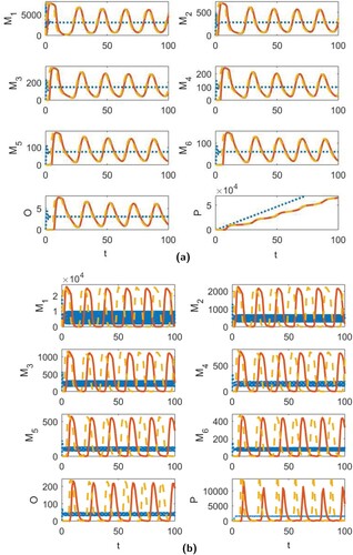
Figure 4. The transient dynamics for the continuous-time model for (a) the parameters in Figure 2(a) (left) and Figure 2(b) (right), and (b) the parameters in Figure 3(a) (left) and Figure 3(b) (right). The cycles obtained in Figure 3(b) for model (1(1) $\begin{array}{rl}\frac{\mathrm{d}{M}_1\left(t\right)}{\mathrm{d}t}& =\delta M_1\left(t\right)\left(1-\frac{M_1\left(t\right)}{\gamma }\right)-2K_1{M}_1^2\left(t\right)-M_1\left(t\right)\sum _{i=2}^{n-1}{K}_i{M}_i\left(t\right),\\ & -(O_a-n)K_n{M}_1\left(t\right)M_n\left(t\right)-(P_a-O_a)K_O{M}_1\left(t\right)O\left(t\right)-{\mu }_1{M}_1\left(t\right),\\ \frac{\mathrm{d}{M}_2\left(t\right)}{\mathrm{d}t}& =K_1{M}_1^2\left(t\right)-K_2{M}_1\left(t\right)M_2\left(t\right)-{\mu }_2{M}_2\left(t\right),\\ & ⋮\\ \frac{\mathrm{d}{M}_n\left(t\right)}{\mathrm{d}t}& =K_{n-1}{M}_1\left(t\right)M_{n-1}\left(t\right)-K_n{M}_1\left(t\right)M_n\left(t\right)-{\mu }_n{M}_n\left(t\right),\\ \frac{\mathrm{d}O\left(t\right)}{\mathrm{d}t}& =K_n{M}_1\left(t\right)M_n\left(t\right)-K_O{M}_1\left(t\right)O\left(t\right)-{\mu }_{O}O\left(t\right),\\ \frac{\mathrm{d}P\left(t\right)}{\mathrm{d}t}& =K_O{M}_1\left(t\right)O\left(t\right)-{\mu }_{P}P\left(t\right).\end{array}$(1) ) are shown in (c) for stage $M_1$.

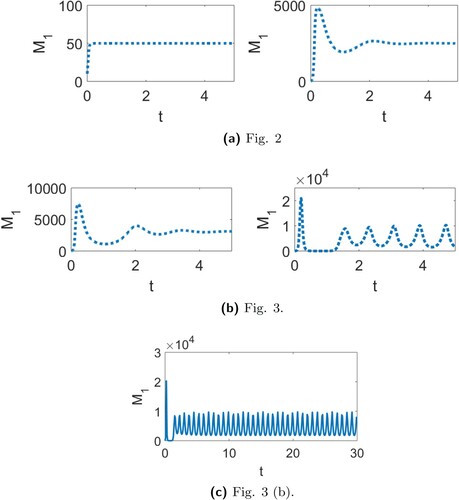
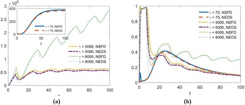
Figure 5. The absolute (a) and relative (b) errors in mass concentration over time for the NSFD model (A1(A1) $\begin{array}{rl}{M}_1(t+1)& =(1+\delta )M_1\left(t\right)\left[1+{\mu }_1+\frac{\delta }{\gamma }{M}_1\left(t\right)+2K_1{M}_1\left(t\right)+\sum _{i=2}^{n-1}{K}_i{M}_i\left(t\right)\right.\\ & {\left.+(O_a-n)K_n{M}_n\left(t\right)+(P_a-O_a)K_{O}O\left(t\right)\phantom{\frac{1}{2}}\right]}^{-1},\\ M_2(t+1)& =\frac{M_2\left(t\right)+K_1{M}_1^2\left(t\right)}{1+{\mu }_2+K_2{M}_1\left(t\right)},\\ M_3(t+1)& =\frac{M_3\left(t\right)+K_2{M}_1\left(t\right)M_2\left(t\right)}{1+{\mu }_3+K_3{M}_1\left(t\right)},\\ & ⋮\\ M_n(t+1)& =\frac{M_n\left(t\right)+K_{n-1}{M}_1\left(t\right)M_{n-1}\left(t\right)}{1+{\mu }_n+K_n{M}_1\left(t\right)},\\ O(t+1)& =\frac{O\left(t\right)+K_n{M}_1\left(t\right)M_n\left(t\right)}{1+{\mu }_O+K_O{M}_1\left(t\right)},\\ P(t+1)& =\frac{P\left(t\right)+K_O{M}_1\left(t\right)O\left(t\right)}{1+{\mu }_P}.\end{array}$(A1) ) and the NEDS model (A2(A2) $\begin{array}{rl}{M}_1(t+1)& =e^{(\delta -{\mu }_1)}{M}_1\left(t\right)\left[1+{\varphi }_1\left(1\right)\left(\frac{\delta }{\gamma }{M}_1\left(t\right)+2K_1{M}_1\left(t\right)+\sum _{i=2}^{n-1}{K}_i{M}_i\left(t\right)\right.\right.\\ & {\left.\left.+(O_a-n)K_n{M}_n\left(t\right)+(P_a-O_a)K_{O}O\left(t\right)\phantom{\frac{1}{2}}\right)\right]}^{-1},\\ M_2(t+1)& =\frac{e^{-{\mu }_2}{M}_2\left(t\right)+{\varphi }_2\left(1\right)K_1{M}_1^2\left(t\right)}{1+{\varphi }_2\left(1\right)K_2{M}_1\left(t\right))},\\ M_3(t+1)& =\frac{e^{-{\mu }_3}{M}_3\left(t\right)+{\varphi }_3\left(1\right)K_2{M}_1\left(t\right)M_2\left(t\right)}{1+{\varphi }_3\left(1\right)K_3{M}_1\left(t\right))},\\ & ⋮\\ M_n(t+1)& =\frac{e^{-{\mu }_n}{M}_n\left(t\right)+{\varphi }_n\left(1\right)K_{n-1}{M}_1\left(t\right)M_{n-1}\left(t\right)}{1+{\varphi }_n\left(1\right)K_n{M}_1\left(t\right))},\\ O(t+1)& =\frac{e^{-{\mu }_O}O\left(t\right)+{\varphi }_O\left(1\right)K_n{M}_1\left(t\right)M_n\left(t\right)}{1+{\varphi }_O\left(1\right)K_O{M}_1\left(t\right)},\\ P(t+1)& =e^{-{\mu }_P}P\left(t\right)+{\varphi }_P\left(1\right)K_O{M}_1\left(t\right)O\left(t\right).\end{array}$(A2) ) for the parameters values given in Figure 2(a) with $\gamma =75$, Figure 2(b) with $\gamma =5000$ and Figure 3(a) with $\gamma =8000$.

Though we were unable to find stable oscillations in the solution to the continuous-time model for the parameter ranges given in Table 1, it is possible for this model to exhibit stable cycles for parameters outside of these ranges. This is demonstrated in Figure 3(b) where $\gamma =30,000$ and all other parameters are the same as Figure 3(a) except we have taken $K_O=0.01$ and ${\mu }_1=\cdots ={\mu }_n={\mu }_O={\mu }_P=1$. In Figure 4, we provide the transient solution to $M_1$ for the continuous-time model for each of the four scenarios considered in Figures 2 and 3. We note that the continuous-time model exhibits some transient oscillations for the parameter values in Figures 2(b) and 3(a), but these oscillations are less significant when compared to the oscillations observed in the discrete-time models. In Figure 4(c), we provide a clearer view of the cycles shown in Figure 3(b) for the continuous-time model.

As discussed in the appendix, the two discrete-time approximations (A1(A1) $\begin{array}{rl}{M}_1(t+1)& =(1+\delta )M_1\left(t\right)\left[1+{\mu }_1+\frac{\delta }{\gamma }{M}_1\left(t\right)+2K_1{M}_1\left(t\right)+\sum _{i=2}^{n-1}{K}_i{M}_i\left(t\right)\right.\\ & {\left.+(O_a-n)K_n{M}_n\left(t\right)+(P_a-O_a)K_{O}O\left(t\right)\phantom{\frac{1}{2}}\right]}^{-1},\\ M_2(t+1)& =\frac{M_2\left(t\right)+K_1{M}_1^2\left(t\right)}{1+{\mu }_2+K_2{M}_1\left(t\right)},\\ M_3(t+1)& =\frac{M_3\left(t\right)+K_2{M}_1\left(t\right)M_2\left(t\right)}{1+{\mu }_3+K_3{M}_1\left(t\right)},\\ & ⋮\\ M_n(t+1)& =\frac{M_n\left(t\right)+K_{n-1}{M}_1\left(t\right)M_{n-1}\left(t\right)}{1+{\mu }_n+K_n{M}_1\left(t\right)},\\ O(t+1)& =\frac{O\left(t\right)+K_n{M}_1\left(t\right)M_n\left(t\right)}{1+{\mu }_O+K_O{M}_1\left(t\right)},\\ P(t+1)& =\frac{P\left(t\right)+K_O{M}_1\left(t\right)O\left(t\right)}{1+{\mu }_P}.\end{array}$(A1) ) and (A2(A2) $\begin{array}{rl}{M}_1(t+1)& =e^{(\delta -{\mu }_1)}{M}_1\left(t\right)\left[1+{\varphi }_1\left(1\right)\left(\frac{\delta }{\gamma }{M}_1\left(t\right)+2K_1{M}_1\left(t\right)+\sum _{i=2}^{n-1}{K}_i{M}_i\left(t\right)\right.\right.\\ & {\left.\left.+(O_a-n)K_n{M}_n\left(t\right)+(P_a-O_a)K_{O}O\left(t\right)\phantom{\frac{1}{2}}\right)\right]}^{-1},\\ M_2(t+1)& =\frac{e^{-{\mu }_2}{M}_2\left(t\right)+{\varphi }_2\left(1\right)K_1{M}_1^2\left(t\right)}{1+{\varphi }_2\left(1\right)K_2{M}_1\left(t\right))},\\ M_3(t+1)& =\frac{e^{-{\mu }_3}{M}_3\left(t\right)+{\varphi }_3\left(1\right)K_2{M}_1\left(t\right)M_2\left(t\right)}{1+{\varphi }_3\left(1\right)K_3{M}_1\left(t\right))},\\ & ⋮\\ M_n(t+1)& =\frac{e^{-{\mu }_n}{M}_n\left(t\right)+{\varphi }_n\left(1\right)K_{n-1}{M}_1\left(t\right)M_{n-1}\left(t\right)}{1+{\varphi }_n\left(1\right)K_n{M}_1\left(t\right))},\\ O(t+1)& =\frac{e^{-{\mu }_O}O\left(t\right)+{\varphi }_O\left(1\right)K_n{M}_1\left(t\right)M_n\left(t\right)}{1+{\varphi }_O\left(1\right)K_O{M}_1\left(t\right)},\\ P(t+1)& =e^{-{\mu }_P}P\left(t\right)+{\varphi }_P\left(1\right)K_O{M}_1\left(t\right)O\left(t\right).\end{array}$(A2) ) do not preserve the mass conservation property of the continuous model (see Lemma 2.1). Specifically, for both discrete-time models, mass is lost in the aggregation process. We suspect that this loss of mass is the cause of the instability observed in the numerical simulations. In Figure 5, we demonstrate how much mass is lost for the scenarios presented in Figures 2 and 3. In Figure 5(a), we plot the absolute error between the total mass concentration over time, as given by the solution to (2(2) $\sum _{i=1}^{n}i\frac{\mathrm{d}{M}_i}{\mathrm{d}t}+O_a\frac{\mathrm{d}O}{\mathrm{d}t}+P_a\frac{\mathrm{d}P}{\mathrm{d}t}=\delta M_1\left(1-\frac{M_1}{\gamma }\right)-\sum _{i=1}^{n}i{\mu }_i{M}_i-O_a{\mu }_{O}O-P_a{\mu }_{P}P.$(2) ), and the mass concentration over time as predicted by models (A1(A1) $\begin{array}{rl}{M}_1(t+1)& =(1+\delta )M_1\left(t\right)\left[1+{\mu }_1+\frac{\delta }{\gamma }{M}_1\left(t\right)+2K_1{M}_1\left(t\right)+\sum _{i=2}^{n-1}{K}_i{M}_i\left(t\right)\right.\\ & {\left.+(O_a-n)K_n{M}_n\left(t\right)+(P_a-O_a)K_{O}O\left(t\right)\phantom{\frac{1}{2}}\right]}^{-1},\\ M_2(t+1)& =\frac{M_2\left(t\right)+K_1{M}_1^2\left(t\right)}{1+{\mu }_2+K_2{M}_1\left(t\right)},\\ M_3(t+1)& =\frac{M_3\left(t\right)+K_2{M}_1\left(t\right)M_2\left(t\right)}{1+{\mu }_3+K_3{M}_1\left(t\right)},\\ & ⋮\\ M_n(t+1)& =\frac{M_n\left(t\right)+K_{n-1}{M}_1\left(t\right)M_{n-1}\left(t\right)}{1+{\mu }_n+K_n{M}_1\left(t\right)},\\ O(t+1)& =\frac{O\left(t\right)+K_n{M}_1\left(t\right)M_n\left(t\right)}{1+{\mu }_O+K_O{M}_1\left(t\right)},\\ P(t+1)& =\frac{P\left(t\right)+K_O{M}_1\left(t\right)O\left(t\right)}{1+{\mu }_P}.\end{array}$(A1) ) and (A2(A2) $\begin{array}{rl}{M}_1(t+1)& =e^{(\delta -{\mu }_1)}{M}_1\left(t\right)\left[1+{\varphi }_1\left(1\right)\left(\frac{\delta }{\gamma }{M}_1\left(t\right)+2K_1{M}_1\left(t\right)+\sum _{i=2}^{n-1}{K}_i{M}_i\left(t\right)\right.\right.\\ & {\left.\left.+(O_a-n)K_n{M}_n\left(t\right)+(P_a-O_a)K_{O}O\left(t\right)\phantom{\frac{1}{2}}\right)\right]}^{-1},\\ M_2(t+1)& =\frac{e^{-{\mu }_2}{M}_2\left(t\right)+{\varphi }_2\left(1\right)K_1{M}_1^2\left(t\right)}{1+{\varphi }_2\left(1\right)K_2{M}_1\left(t\right))},\\ M_3(t+1)& =\frac{e^{-{\mu }_3}{M}_3\left(t\right)+{\varphi }_3\left(1\right)K_2{M}_1\left(t\right)M_2\left(t\right)}{1+{\varphi }_3\left(1\right)K_3{M}_1\left(t\right))},\\ & ⋮\\ M_n(t+1)& =\frac{e^{-{\mu }_n}{M}_n\left(t\right)+{\varphi }_n\left(1\right)K_{n-1}{M}_1\left(t\right)M_{n-1}\left(t\right)}{1+{\varphi }_n\left(1\right)K_n{M}_1\left(t\right))},\\ O(t+1)& =\frac{e^{-{\mu }_O}O\left(t\right)+{\varphi }_O\left(1\right)K_n{M}_1\left(t\right)M_n\left(t\right)}{1+{\varphi }_O\left(1\right)K_O{M}_1\left(t\right)},\\ P(t+1)& =e^{-{\mu }_P}P\left(t\right)+{\varphi }_P\left(1\right)K_O{M}_1\left(t\right)O\left(t\right).\end{array}$(A2) ). As we can see from this figure, model (A2(A2) $\begin{array}{rl}{M}_1(t+1)& =e^{(\delta -{\mu }_1)}{M}_1\left(t\right)\left[1+{\varphi }_1\left(1\right)\left(\frac{\delta }{\gamma }{M}_1\left(t\right)+2K_1{M}_1\left(t\right)+\sum _{i=2}^{n-1}{K}_i{M}_i\left(t\right)\right.\right.\\ & {\left.\left.+(O_a-n)K_n{M}_n\left(t\right)+(P_a-O_a)K_{O}O\left(t\right)\phantom{\frac{1}{2}}\right)\right]}^{-1},\\ M_2(t+1)& =\frac{e^{-{\mu }_2}{M}_2\left(t\right)+{\varphi }_2\left(1\right)K_1{M}_1^2\left(t\right)}{1+{\varphi }_2\left(1\right)K_2{M}_1\left(t\right))},\\ M_3(t+1)& =\frac{e^{-{\mu }_3}{M}_3\left(t\right)+{\varphi }_3\left(1\right)K_2{M}_1\left(t\right)M_2\left(t\right)}{1+{\varphi }_3\left(1\right)K_3{M}_1\left(t\right))},\\ & ⋮\\ M_n(t+1)& =\frac{e^{-{\mu }_n}{M}_n\left(t\right)+{\varphi }_n\left(1\right)K_{n-1}{M}_1\left(t\right)M_{n-1}\left(t\right)}{1+{\varphi }_n\left(1\right)K_n{M}_1\left(t\right))},\\ O(t+1)& =\frac{e^{-{\mu }_O}O\left(t\right)+{\varphi }_O\left(1\right)K_n{M}_1\left(t\right)M_n\left(t\right)}{1+{\varphi }_O\left(1\right)K_O{M}_1\left(t\right)},\\ P(t+1)& =e^{-{\mu }_P}P\left(t\right)+{\varphi }_P\left(1\right)K_O{M}_1\left(t\right)O\left(t\right).\end{array}$(A2) ) does a slightly better job than model (A1(A1) $\begin{array}{rl}{M}_1(t+1)& =(1+\delta )M_1\left(t\right)\left[1+{\mu }_1+\frac{\delta }{\gamma }{M}_1\left(t\right)+2K_1{M}_1\left(t\right)+\sum _{i=2}^{n-1}{K}_i{M}_i\left(t\right)\right.\\ & {\left.+(O_a-n)K_n{M}_n\left(t\right)+(P_a-O_a)K_{O}O\left(t\right)\phantom{\frac{1}{2}}\right]}^{-1},\\ M_2(t+1)& =\frac{M_2\left(t\right)+K_1{M}_1^2\left(t\right)}{1+{\mu }_2+K_2{M}_1\left(t\right)},\\ M_3(t+1)& =\frac{M_3\left(t\right)+K_2{M}_1\left(t\right)M_2\left(t\right)}{1+{\mu }_3+K_3{M}_1\left(t\right)},\\ & ⋮\\ M_n(t+1)& =\frac{M_n\left(t\right)+K_{n-1}{M}_1\left(t\right)M_{n-1}\left(t\right)}{1+{\mu }_n+K_n{M}_1\left(t\right)},\\ O(t+1)& =\frac{O\left(t\right)+K_n{M}_1\left(t\right)M_n\left(t\right)}{1+{\mu }_O+K_O{M}_1\left(t\right)},\\ P(t+1)& =\frac{P\left(t\right)+K_O{M}_1\left(t\right)O\left(t\right)}{1+{\mu }_P}.\end{array}$(A1) ) at preserving mass. In Figure 5(b), we give the relative error for both models. Here we observe that, as we move further away from stability condition (10(10) $\sum _{i=2}^{n-1}{K}_i+(O_a-n)K_n+(P_a-O_a)K_O<\frac{\delta }{\gamma }+2K_1.$(10) ) by increasing γ, the relative error in mass concentration increases.

4.1. Sensitivity analysis

Sensitivity analysis plays an important role in parameter estimation and optimization [1–3] and uncertainty [4,21]. Sensitivity analysis involves studying the effects of varying model parameters on the model output. For our model, this involves understanding the $(n+2)\times (2n+5)$ sensitivity coefficient matrix given by $C_S=\frac{\mathrm{d}M}{\mathrm{d}p},$where for convenience we denote $M=(M_1,\dots ,M_n,O,P)\mathrm{a}\mathrm{n}\mathrm{d}p=(\delta ,\gamma ,K_1,\dots ,K_n,K_O,{\mu }_1,\dots ,{\mu }_n,{\mu }_O,{\mu }_P).$Because our model parameters are measured in different units and differ by orders of magnitude, this presents a challenge in interpreting sensitivity results and makes it difficult to compare sensitivities between different parameters. Thus we focus on elasticity analysis as it is a more appropriate measure in such a case [12]. Elasticity analysis looks at the proportional response to a proportional (rather than additive) change in a model parameter. The elasticity coefficient matrix is given by $C_E=\frac{\mathrm{d}M}{\mathrm{d}p}\frac{p}{M}.$In particular, elasticities are proportional sensitivities that are scaled so that they are dimensionless. Thus one can directly compare elasticities among all model parameters.

Here, we use a simple finite difference to approximate the derivative and numerically solve for the elasticity coefficient matrix. Specifically, we use the following scheme to numerically compute these elasticity coefficients $\left(C_E{)}_{i,j}\right(t;p)=\frac{\mathrm{\partial }{M}_i(t;p)}{\mathrm{\partial }{p}_j}\frac{p_j}{M_i(t,p)}\approx \left(\frac{M_i(t;p+\mathrm{\Delta }{p}_j)-M_i(t;p)}{\mathrm{\Delta }{p}_j}\right)\frac{p_j}{M_i(t,p)},$for $i=1,\dots ,n+2,j=1,\dots ,2n+5$ and small $\mathrm{\Delta }{p}_j>0$.

In Figure 6, we present the elasticity of the concentration of aggregates over time with respect to three parameters: $K_1$, $K_2$ and γ. This graph was generated using the same parameter values as Figure 2(a) and gives the absolute value of the elasticities in order to more easily compare their relative magnitudes. From Figure 6, we can observe both the transient effects, which contribute to the time it takes different stages to equilibrate, as well as the asymptotic effects, which describe how model parameters impact final equilibrium concentrations. Similar qualitative behaviour is observed for other parameters but the magnitude (elasticity level) changes from one parameter to another. Thus in Table 2 we present the transpose of the full elasticity coefficient matrix at the final time of the simulation T = 800, i.e. the transpose of $C_E(T;p)$. Since n = 6 this matrix is of dimension $17\times 8$. This table clearly demonstrates that aggregate equilibrium concentrations are most sensitive to γ, followed by $K_1$. In general, we also observe that, when comparing the effects of different elongation or degradation rates, the model outputs are more sensitive to the rate with a lower index. Exceptions occur for the stage that rate directly impacts, for instance changes in $K_4$ have a greater impact on $M_4$ than changes in $K_2$ or $K_3$. For comparison purposes, we also computed the elasticities when γ is increased to $\gamma =5000$ as in Figure 2(b) (not shown). These elasticities show the same general pattern as is given in Table 2 except that the impact of δ is increased, with the elasticities with respect to δ and γ having the same order of magnitude.

Figure 6. The elasticity of the concentration of aggregates over time with respect to $K_1$ (solid blue line), $K_2$ (red dashed line), and γ (yellow dotted line). Parameter values are the same as those used in Figure 2(a).

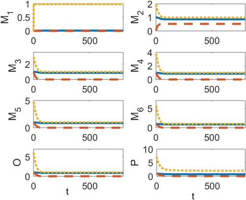
Table 2. The transpose of the elasticity coefficient matrix at T = 800 for the model (1(1) $\begin{array}{rl}\frac{\mathrm{d}{M}_1\left(t\right)}{\mathrm{d}t}& =\delta M_1\left(t\right)\left(1-\frac{M_1\left(t\right)}{\gamma }\right)-2K_1{M}_1^2\left(t\right)-M_1\left(t\right)\sum _{i=2}^{n-1}{K}_i{M}_i\left(t\right),\\ & -(O_a-n)K_n{M}_1\left(t\right)M_n\left(t\right)-(P_a-O_a)K_O{M}_1\left(t\right)O\left(t\right)-{\mu }_1{M}_1\left(t\right),\\ \frac{\mathrm{d}{M}_2\left(t\right)}{\mathrm{d}t}& =K_1{M}_1^2\left(t\right)-K_2{M}_1\left(t\right)M_2\left(t\right)-{\mu }_2{M}_2\left(t\right),\\ & ⋮\\ \frac{\mathrm{d}{M}_n\left(t\right)}{\mathrm{d}t}& =K_{n-1}{M}_1\left(t\right)M_{n-1}\left(t\right)-K_n{M}_1\left(t\right)M_n\left(t\right)-{\mu }_n{M}_n\left(t\right),\\ \frac{\mathrm{d}O\left(t\right)}{\mathrm{d}t}& =K_n{M}_1\left(t\right)M_n\left(t\right)-K_O{M}_1\left(t\right)O\left(t\right)-{\mu }_{O}O\left(t\right),\\ \frac{\mathrm{d}P\left(t\right)}{\mathrm{d}t}& =K_O{M}_1\left(t\right)O\left(t\right)-{\mu }_{P}P\left(t\right).\end{array}$(1) ).

Elasticity w.r.t.	$M_1$	$M_2$	$M_3$	$M_4$	$M_5$	$M_6$	O	P
δ	1.46$\times {10}^{-2}$	1.47$\times {10}^{-2}$	1.48$\times {10}^{-2}$	1.48$\times {10}^{-2}$	1.48$\times {10}^{-2}$	1.48$\times {10}^{-2}$	1.48$\times {10}^{-2}$	2.90$\times {10}^{-2}$
γ	9.85$\times {10}^{-1}$	9.91$\times {10}^{-1}$	9.93$\times {10}^{-1}$	9.94$\times {10}^{-1}$	9.95$\times {10}^{-1}$	9.96$\times {10}^{-1}$	9.96$\times {10}^{-1}$	2.02$\times {10}^0$
$K_1$	−1.27$\times {10}^{-2}$	8.59$\times {10}^{-1}$	8.59$\times {10}^{-1}$	8.58$\times {10}^{-1}$	8.58$\times {10}^{-1}$	8.58$\times {10}^{-1}$	8.58$\times {10}^{-1}$	7.40$\times {10}^{-1}$
$K_2$	−4.60$\times {10}^{-5}$	−5.22$\times {10}^{-1}$	3.17$\times {10}^{-3}$	3.16$\times {10}^{-3}$	3.16$\times {10}^{-3}$	3.16$\times {10}^{-3}$	3.16$\times {10}^{-3}$	1.11$\times {10}^{-2}$
$K_3$	−2.06$\times {10}^{-5}$	−2.07$\times {10}^{-5}$	−6.76$\times {10}^{-1}$	1.43$\times {10}^{-3}$	1.43$\times {10}^{-3}$	1.43$\times {10}^{-3}$	1.43$\times {10}^{-3}$	6.87$\times {10}^{-3}$
$K_4$	−1.16$\times {10}^{-5}$	−1.16$\times {10}^{-5}$	−1.17$\times {10}^{-5}$	−7.55$\times {10}^{-1}$	8.13$\times {10}^{-4}$	8.13$\times {10}^{-4}$	8.13$\times {10}^{-4}$	4.94$\times {10}^{-3}$
$K_5$	−7.37$\times {10}^{-6}$	−7.41$\times {10}^{-6}$	−7.43$\times {10}^{-6}$	−7.44$\times {10}^{-6}$	−8.04$\times {10}^{-1}$	5.23$\times {10}^{-4}$	5.23$\times {10}^{-4}$	3.84$\times {10}^{-3}$
$K_6$	−5.08$\times {10}^{-6}$	−5.11$\times {10}^{-6}$	−5.12$\times {10}^{-6}$	−5.13$\times {10}^{-6}$	−5.13$\times {10}^{-6}$	−8.36$\times {10}^{-1}$	3.64$\times {10}^{-4}$	3.14$\times {10}^{-3}$
$K_O$	−1.76$\times {10}^{-7}$	−1.77$\times {10}^{-7}$	−1.78$\times {10}^{-7}$	−1.78$\times {10}^{-7}$	−1.78$\times {10}^{-7}$	−1.78$\times {10}^{-7}$	−9.90$\times {10}^{-1}$	1.81$\times {10}^{-4}$
${\mu }_1$	−2.00$\times {10}^{-5}$	−2.01$\times {10}^{-5}$	−2.02$\times {10}^{-5}$	−2.02$\times {10}^{-5}$	−2.02$\times {10}^{-5}$	−2.02$\times {10}^{-5}$	−2.02$\times {10}^{-5}$	−4.09$\times {10}^{-5}$
${\mu }_2$	8.66$\times {10}^{-5}$	−5.95$\times {10}^{-3}$	−5.95$\times {10}^{-3}$	−5.95$\times {10}^{-3}$	−5.95$\times {10}^{-3}$	−5.95$\times {10}^{-3}$	−5.95$\times {10}^{-3}$	−5.78$\times {10}^{-3}$
${\mu }_3$	3.02$\times {10}^{-5}$	3.04$\times {10}^{-5}$	−2.10$\times {10}^{-3}$	−2.10$\times {10}^{-3}$	−2.10$\times {10}^{-3}$	−2.10$\times {10}^{-3}$	−2.10$\times {10}^{-3}$	−2.05$\times {10}^{-3}$
${\mu }_4$	1.52$\times {10}^{-5}$	1.53$\times {10}^{-5}$	1.54$\times {10}^{-5}$	−1.07$\times {10}^{-3}$	−1.07$\times {10}^{-3}$	−1.07$\times {10}^{-3}$	−1.07$\times {10}^{-3}$	−1.05$\times {10}^{-3}$
${\mu }_5$	9.13$\times {10}^{-6}$	9.19$\times {10}^{-6}$	9.21$\times {10}^{-6}$	9.22$\times {10}^{-6}$	−6.48$\times {10}^{-4}$	−6.48$\times {10}^{-4}$	−6.48$\times {10}^{-4}$	−6.37$\times {10}^{-4}$
${\mu }_6$	6.06$\times {10}^{-6}$	6.10$\times {10}^{-6}$	6.11$\times {10}^{-6}$	6.12$\times {10}^{-6}$	6.12$\times {10}^{-6}$	−4.35$\times {10}^{-4}$	−4.35$\times {10}^{-4}$	−4.27$\times {10}^{-4}$
${\mu }_O$	1.78$\times {10}^{-7}$	1.79$\times {10}^{-7}$	1.80$\times {10}^{-7}$	1.80$\times {10}^{-7}$	1.80$\times {10}^{-7}$	1.80$\times {10}^{-7}$	−1.33$\times {10}^{-5}$	−1.32$\times {10}^{-5}$
${\mu }_P$	8.85$\times {10}^{-17}$	−8.55$\times {10}^{-16}$	−2.06$\times {10}^{-15}$	−3.34$\times {10}^{-15}$	−4.50$\times {10}^{-15}$	−5.95$\times {10}^{-15}$	−6.02$\times {10}^{-15}$	−3.03$\times {10}^{-3}$

5. Conclusion

In this paper, we developed a continuous-time model for the aggregation of Aβ. This model uses size (in term of the number of monomers) to model the slow nucleation phase and stage to model the faster elongation phase. Motivated by previous studies [73], the model also explicitly distinguishes between oligomer and fibril stages, and their elongation rates. The main limitation of this new model is that we assume oligomers and fibrils can be well characterized by average sizes for each of these stages. While describing a group according average characteristics is a common approach in stage-structured population modelling, such an approach may not be appropriate when there is a large amount of variability within a group. For instance, model (1(1) $\begin{array}{rl}\frac{\mathrm{d}{M}_1\left(t\right)}{\mathrm{d}t}& =\delta M_1\left(t\right)\left(1-\frac{M_1\left(t\right)}{\gamma }\right)-2K_1{M}_1^2\left(t\right)-M_1\left(t\right)\sum _{i=2}^{n-1}{K}_i{M}_i\left(t\right),\\ & -(O_a-n)K_n{M}_1\left(t\right)M_n\left(t\right)-(P_a-O_a)K_O{M}_1\left(t\right)O\left(t\right)-{\mu }_1{M}_1\left(t\right),\\ \frac{\mathrm{d}{M}_2\left(t\right)}{\mathrm{d}t}& =K_1{M}_1^2\left(t\right)-K_2{M}_1\left(t\right)M_2\left(t\right)-{\mu }_2{M}_2\left(t\right),\\ & ⋮\\ \frac{\mathrm{d}{M}_n\left(t\right)}{\mathrm{d}t}& =K_{n-1}{M}_1\left(t\right)M_{n-1}\left(t\right)-K_n{M}_1\left(t\right)M_n\left(t\right)-{\mu }_n{M}_n\left(t\right),\\ \frac{\mathrm{d}O\left(t\right)}{\mathrm{d}t}& =K_n{M}_1\left(t\right)M_n\left(t\right)-K_O{M}_1\left(t\right)O\left(t\right)-{\mu }_{O}O\left(t\right),\\ \frac{\mathrm{d}P\left(t\right)}{\mathrm{d}t}& =K_O{M}_1\left(t\right)O\left(t\right)-{\mu }_{P}P\left(t\right).\end{array}$(1) ) may be more appropriate for describing the early stages of AD progression, while, for later stages of AD, an extension of this model in which we include multiple oligomer and fibril stages may work better.

We showed that the continuous-time model (1(1) $\begin{array}{rl}\frac{\mathrm{d}{M}_1\left(t\right)}{\mathrm{d}t}& =\delta M_1\left(t\right)\left(1-\frac{M_1\left(t\right)}{\gamma }\right)-2K_1{M}_1^2\left(t\right)-M_1\left(t\right)\sum _{i=2}^{n-1}{K}_i{M}_i\left(t\right),\\ & -(O_a-n)K_n{M}_1\left(t\right)M_n\left(t\right)-(P_a-O_a)K_O{M}_1\left(t\right)O\left(t\right)-{\mu }_1{M}_1\left(t\right),\\ \frac{\mathrm{d}{M}_2\left(t\right)}{\mathrm{d}t}& =K_1{M}_1^2\left(t\right)-K_2{M}_1\left(t\right)M_2\left(t\right)-{\mu }_2{M}_2\left(t\right),\\ & ⋮\\ \frac{\mathrm{d}{M}_n\left(t\right)}{\mathrm{d}t}& =K_{n-1}{M}_1\left(t\right)M_{n-1}\left(t\right)-K_n{M}_1\left(t\right)M_n\left(t\right)-{\mu }_n{M}_n\left(t\right),\\ \frac{\mathrm{d}O\left(t\right)}{\mathrm{d}t}& =K_n{M}_1\left(t\right)M_n\left(t\right)-K_O{M}_1\left(t\right)O\left(t\right)-{\mu }_{O}O\left(t\right),\\ \frac{\mathrm{d}P\left(t\right)}{\mathrm{d}t}& =K_O{M}_1\left(t\right)O\left(t\right)-{\mu }_{P}P\left(t\right).\end{array}$(1) ) has an extinction equilibrium and a unique positive equilibrium, and applied Gershgorin's Theorem to establish local stability. Numerical simulations show that, for parameter values falling within biologically reasonable ranges, this model exhibits the sigmoidal growth, Figure 2(a), that is predicted by theory [37]. These simulations also show that the stability region for the positive equilibrium extends beyond the stability region, determined by condition (10(10) $\sum _{i=2}^{n-1}{K}_i+(O_a-n)K_n+(P_a-O_a)K_O<\frac{\delta }{\gamma }+2K_1.$(10) ), established in Theorem 3.3. We conjecture that the positive equilibrium may, in fact, be globally asymptotically stable and we aim to establish conditions on the model parameters for global stability in future work. However, we point out that the stability of the positive equilibrium is not always guaranteed, as is demonstrated by the numerical results in Figure 3(b) and Figure 4(c) which show that the model may exhibit more complicated dynamics including periodicity of solutions. It is worth noting, however, that these oscillations were obtained using parameter values outside of the ranges given in Table 1. Meanwhile, numerical simulations suggest that the continuous-time model does not appear to exhibit oscillations when parameter values are chosen from the biological ranges provided in Table 1.

Other approaches, including discrete-time models [20], have been used to model Aβ aggregation. In order to compare how model predictions may vary based on the approach used, here we also developed two discrete-time approximations to the model (1(1) $\begin{array}{rl}\frac{\mathrm{d}{M}_1\left(t\right)}{\mathrm{d}t}& =\delta M_1\left(t\right)\left(1-\frac{M_1\left(t\right)}{\gamma }\right)-2K_1{M}_1^2\left(t\right)-M_1\left(t\right)\sum _{i=2}^{n-1}{K}_i{M}_i\left(t\right),\\ & -(O_a-n)K_n{M}_1\left(t\right)M_n\left(t\right)-(P_a-O_a)K_O{M}_1\left(t\right)O\left(t\right)-{\mu }_1{M}_1\left(t\right),\\ \frac{\mathrm{d}{M}_2\left(t\right)}{\mathrm{d}t}& =K_1{M}_1^2\left(t\right)-K_2{M}_1\left(t\right)M_2\left(t\right)-{\mu }_2{M}_2\left(t\right),\\ & ⋮\\ \frac{\mathrm{d}{M}_n\left(t\right)}{\mathrm{d}t}& =K_{n-1}{M}_1\left(t\right)M_{n-1}\left(t\right)-K_n{M}_1\left(t\right)M_n\left(t\right)-{\mu }_n{M}_n\left(t\right),\\ \frac{\mathrm{d}O\left(t\right)}{\mathrm{d}t}& =K_n{M}_1\left(t\right)M_n\left(t\right)-K_O{M}_1\left(t\right)O\left(t\right)-{\mu }_{O}O\left(t\right),\\ \frac{\mathrm{d}P\left(t\right)}{\mathrm{d}t}& =K_O{M}_1\left(t\right)O\left(t\right)-{\mu }_{P}P\left(t\right).\end{array}$(1) ) using non-standard schemes. We showed that these models preserve the local dynamics of the continuous-time model. Numerical simulations verify that, even outside of the stability region determined by (10(10) $\sum _{i=2}^{n-1}{K}_i+(O_a-n)K_n+(P_a-O_a)K_O<\frac{\delta }{\gamma }+2K_1.$(10) ), these difference schemes may provide good approximations to model (1(1) $\begin{array}{rl}\frac{\mathrm{d}{M}_1\left(t\right)}{\mathrm{d}t}& =\delta M_1\left(t\right)\left(1-\frac{M_1\left(t\right)}{\gamma }\right)-2K_1{M}_1^2\left(t\right)-M_1\left(t\right)\sum _{i=2}^{n-1}{K}_i{M}_i\left(t\right),\\ & -(O_a-n)K_n{M}_1\left(t\right)M_n\left(t\right)-(P_a-O_a)K_O{M}_1\left(t\right)O\left(t\right)-{\mu }_1{M}_1\left(t\right),\\ \frac{\mathrm{d}{M}_2\left(t\right)}{\mathrm{d}t}& =K_1{M}_1^2\left(t\right)-K_2{M}_1\left(t\right)M_2\left(t\right)-{\mu }_2{M}_2\left(t\right),\\ & ⋮\\ \frac{\mathrm{d}{M}_n\left(t\right)}{\mathrm{d}t}& =K_{n-1}{M}_1\left(t\right)M_{n-1}\left(t\right)-K_n{M}_1\left(t\right)M_n\left(t\right)-{\mu }_n{M}_n\left(t\right),\\ \frac{\mathrm{d}O\left(t\right)}{\mathrm{d}t}& =K_n{M}_1\left(t\right)M_n\left(t\right)-K_O{M}_1\left(t\right)O\left(t\right)-{\mu }_{O}O\left(t\right),\\ \frac{\mathrm{d}P\left(t\right)}{\mathrm{d}t}& =K_O{M}_1\left(t\right)O\left(t\right)-{\mu }_{P}P\left(t\right).\end{array}$(1) ). However, as we move away from this condition, the discrete-time models start to exhibit oscillatory transience and eventually stable cycles. This loss of stability appears to coincide with a loss of conservation of mass, as shown in Figure 5. This suggest that one should use caution when using discrete-time approximations to model aggregation processes.

The onset and progression of Alzheimer's disease can vary greatly between individuals due to factors that are not well understood [6]. In Section 4.1, we performed sensitivity analysis of the model outputs to understand how variability in the parameters describing the aggregation process of Aβ may influence the time series dynamics. When comparing the various elongation rates, we observe that, even after accounting for differences in order of magnitude of parameter values by using elasticity measurements, the impact of these rates on the final equilibrium values may vary by orders of magnitude with the elongation rates of smaller aggregate sizes having a larger impact on equilibrium values. In particular, this suggests that it may be important to have distinct elongation rates for the smaller versus larger aggregates. This was observed experimentally for tau aggregation [73], where the traditional kinetic equations were found to underestimated average fibril length and be inadequate at capturing oligomer concentrations over time. Meanwhile, a model that accounts for the conversion of oligomers to fibrils via a reaction of first order in monomer concentration, as we have in model (1(1) $\begin{array}{rl}\frac{\mathrm{d}{M}_1\left(t\right)}{\mathrm{d}t}& =\delta M_1\left(t\right)\left(1-\frac{M_1\left(t\right)}{\gamma }\right)-2K_1{M}_1^2\left(t\right)-M_1\left(t\right)\sum _{i=2}^{n-1}{K}_i{M}_i\left(t\right),\\ & -(O_a-n)K_n{M}_1\left(t\right)M_n\left(t\right)-(P_a-O_a)K_O{M}_1\left(t\right)O\left(t\right)-{\mu }_1{M}_1\left(t\right),\\ \frac{\mathrm{d}{M}_2\left(t\right)}{\mathrm{d}t}& =K_1{M}_1^2\left(t\right)-K_2{M}_1\left(t\right)M_2\left(t\right)-{\mu }_2{M}_2\left(t\right),\\ & ⋮\\ \frac{\mathrm{d}{M}_n\left(t\right)}{\mathrm{d}t}& =K_{n-1}{M}_1\left(t\right)M_{n-1}\left(t\right)-K_n{M}_1\left(t\right)M_n\left(t\right)-{\mu }_n{M}_n\left(t\right),\\ \frac{\mathrm{d}O\left(t\right)}{\mathrm{d}t}& =K_n{M}_1\left(t\right)M_n\left(t\right)-K_O{M}_1\left(t\right)O\left(t\right)-{\mu }_{O}O\left(t\right),\\ \frac{\mathrm{d}P\left(t\right)}{\mathrm{d}t}& =K_O{M}_1\left(t\right)O\left(t\right)-{\mu }_{P}P\left(t\right).\end{array}$(1) ), was shown to provide a better fit despite categorizing aggregates into only one of three stages: monomer, oligomer or fibril. We observe a similar pattern was comparing the degradation rates of the different aggregate sizes. All together, we observe that the parameters related to the production δ and prevalence γ of (abnormal) monomers as well as the nucleation rate $K_1$, which leads to the creation of new aggregates, have the greatest effect on both the transient concentrations of aggregates and the final equilibrium concentrations. The sensitivity analysis presented here, together with knowledge on which model parameters are more likely to vary between individuals, may further help identify causes of individual variation in AD progression.

Finally, we note that the model presented in this paper is a first step toward providing a more detailed description of Aβ aggregation that will serve as a basis for more realistic models that account for additional aggregation mechanisms such as dissociation, fragmentation and secondary nucleation. Unlike the traditional kinetic equations that are often used to model Aβ, here we do not assume that the elongation rates for aggregates of different sizes are the same [42]. Without this assumption, the model in this paper has the disadvantage of being less readily analysable. However, the distinction between these rates may prove important for reproducing the results of kinetic studies [73]. In addition, the model is formulated to be flexible enough to allow very detailed information on smaller aggregates which can be experimentally measured. The results of the sensitivity analysis presented in this paper demonstrate the need for having good estimates for some of the model parameters that are highly elastic including parameters that affect the monomer production and monomer nucleation phase. In future work, we plan to estimate model parameters using dynamic light scattering (DLS) data which allows the approximation of aggregate size and molecular weight distribution as a function of time.

Disclosure statement

No potential conflict of interest was reported by the authors.

Appendix. Discrete-Time approximations to the continuous-time model

Various types of mathematical models have been used to describe the aggregation of Aβ or of other proteins. Here we contrast two modelling strategies, specifically continuous versus discrete time, by constructing two discrete-time approximations to the continuous-time model (1(1) $\begin{array}{rl}\frac{\mathrm{d}{M}_1\left(t\right)}{\mathrm{d}t}& =\delta M_1\left(t\right)\left(1-\frac{M_1\left(t\right)}{\gamma }\right)-2K_1{M}_1^2\left(t\right)-M_1\left(t\right)\sum _{i=2}^{n-1}{K}_i{M}_i\left(t\right),\\ & -(O_a-n)K_n{M}_1\left(t\right)M_n\left(t\right)-(P_a-O_a)K_O{M}_1\left(t\right)O\left(t\right)-{\mu }_1{M}_1\left(t\right),\\ \frac{\mathrm{d}{M}_2\left(t\right)}{\mathrm{d}t}& =K_1{M}_1^2\left(t\right)-K_2{M}_1\left(t\right)M_2\left(t\right)-{\mu }_2{M}_2\left(t\right),\\ & ⋮\\ \frac{\mathrm{d}{M}_n\left(t\right)}{\mathrm{d}t}& =K_{n-1}{M}_1\left(t\right)M_{n-1}\left(t\right)-K_n{M}_1\left(t\right)M_n\left(t\right)-{\mu }_n{M}_n\left(t\right),\\ \frac{\mathrm{d}O\left(t\right)}{\mathrm{d}t}& =K_n{M}_1\left(t\right)M_n\left(t\right)-K_O{M}_1\left(t\right)O\left(t\right)-{\mu }_{O}O\left(t\right),\\ \frac{\mathrm{d}P\left(t\right)}{\mathrm{d}t}& =K_O{M}_1\left(t\right)O\left(t\right)-{\mu }_{P}P\left(t\right).\end{array}$(1) ) using non-standard discretization methods.

The first method is based on a nonstandard finite difference discretization (NSFD) (see, e.g.[55]) which preserves the non-negativity of all variables, while the second approximation follows from an exact discretization scheme (NEDS) [44]. Though this latter method is not guaranteed to preserve non-negativity, solutions will remain non-negative provided that the removal terms ${\mu }_i$ are not too large, as is the case here. The main advantage of the discrete-time approximations presented below in comparison with those available in the literature (including Runge–Kutta methods with and without adaptive time step size) is that these approximations are guaranteed to preserve the local dynamics of the continuous system even when the time-step size is large. Specifically, both discrete-time models have the same equilibria and local stability results as the continuous-time model (1(1) $\begin{array}{rl}\frac{\mathrm{d}{M}_1\left(t\right)}{\mathrm{d}t}& =\delta M_1\left(t\right)\left(1-\frac{M_1\left(t\right)}{\gamma }\right)-2K_1{M}_1^2\left(t\right)-M_1\left(t\right)\sum _{i=2}^{n-1}{K}_i{M}_i\left(t\right),\\ & -(O_a-n)K_n{M}_1\left(t\right)M_n\left(t\right)-(P_a-O_a)K_O{M}_1\left(t\right)O\left(t\right)-{\mu }_1{M}_1\left(t\right),\\ \frac{\mathrm{d}{M}_2\left(t\right)}{\mathrm{d}t}& =K_1{M}_1^2\left(t\right)-K_2{M}_1\left(t\right)M_2\left(t\right)-{\mu }_2{M}_2\left(t\right),\\ & ⋮\\ \frac{\mathrm{d}{M}_n\left(t\right)}{\mathrm{d}t}& =K_{n-1}{M}_1\left(t\right)M_{n-1}\left(t\right)-K_n{M}_1\left(t\right)M_n\left(t\right)-{\mu }_n{M}_n\left(t\right),\\ \frac{\mathrm{d}O\left(t\right)}{\mathrm{d}t}& =K_n{M}_1\left(t\right)M_n\left(t\right)-K_O{M}_1\left(t\right)O\left(t\right)-{\mu }_{O}O\left(t\right),\\ \frac{\mathrm{d}P\left(t\right)}{\mathrm{d}t}& =K_O{M}_1\left(t\right)O\left(t\right)-{\mu }_{P}P\left(t\right).\end{array}$(1) ). This is important from a practical point of view as often the step-size represents a generation time or the period of some empirical measurements and hence is fixed.

In our first approach, we approximate the derivatives by $\begin{array}{rl}\frac{\mathrm{d}{M}_i\left(t\right)}{\mathrm{d}t}& \approx \frac{M_i(t+h)-M_i\left(t\right)}{h},i=1,\dots ,n,\\ \frac{\mathrm{d}O\left(t\right)}{\mathrm{d}t}& \approx \frac{O(t+h)-O\left(t\right)}{h},\\ \frac{\mathrm{d}P\left(t\right)}{\mathrm{d}t}& \approx \frac{P(t+h)-P\left(t\right)}{h},\end{array}$with $h=1$. We then apply a non-standard discretization method on the continuous model (1(1) $\begin{array}{rl}\frac{\mathrm{d}{M}_1\left(t\right)}{\mathrm{d}t}& =\delta M_1\left(t\right)\left(1-\frac{M_1\left(t\right)}{\gamma }\right)-2K_1{M}_1^2\left(t\right)-M_1\left(t\right)\sum _{i=2}^{n-1}{K}_i{M}_i\left(t\right),\\ & -(O_a-n)K_n{M}_1\left(t\right)M_n\left(t\right)-(P_a-O_a)K_O{M}_1\left(t\right)O\left(t\right)-{\mu }_1{M}_1\left(t\right),\\ \frac{\mathrm{d}{M}_2\left(t\right)}{\mathrm{d}t}& =K_1{M}_1^2\left(t\right)-K_2{M}_1\left(t\right)M_2\left(t\right)-{\mu }_2{M}_2\left(t\right),\\ & ⋮\\ \frac{\mathrm{d}{M}_n\left(t\right)}{\mathrm{d}t}& =K_{n-1}{M}_1\left(t\right)M_{n-1}\left(t\right)-K_n{M}_1\left(t\right)M_n\left(t\right)-{\mu }_n{M}_n\left(t\right),\\ \frac{\mathrm{d}O\left(t\right)}{\mathrm{d}t}& =K_n{M}_1\left(t\right)M_n\left(t\right)-K_O{M}_1\left(t\right)O\left(t\right)-{\mu }_{O}O\left(t\right),\\ \frac{\mathrm{d}P\left(t\right)}{\mathrm{d}t}& =K_O{M}_1\left(t\right)O\left(t\right)-{\mu }_{P}P\left(t\right).\end{array}$(1) ) as follows. We approximate the quadratic term $-\frac{\delta }{\gamma }M(t{)}^2$ in the first equation of (1(1) $\begin{array}{rl}\frac{\mathrm{d}{M}_1\left(t\right)}{\mathrm{d}t}& =\delta M_1\left(t\right)\left(1-\frac{M_1\left(t\right)}{\gamma }\right)-2K_1{M}_1^2\left(t\right)-M_1\left(t\right)\sum _{i=2}^{n-1}{K}_i{M}_i\left(t\right),\\ & -(O_a-n)K_n{M}_1\left(t\right)M_n\left(t\right)-(P_a-O_a)K_O{M}_1\left(t\right)O\left(t\right)-{\mu }_1{M}_1\left(t\right),\\ \frac{\mathrm{d}{M}_2\left(t\right)}{\mathrm{d}t}& =K_1{M}_1^2\left(t\right)-K_2{M}_1\left(t\right)M_2\left(t\right)-{\mu }_2{M}_2\left(t\right),\\ & ⋮\\ \frac{\mathrm{d}{M}_n\left(t\right)}{\mathrm{d}t}& =K_{n-1}{M}_1\left(t\right)M_{n-1}\left(t\right)-K_n{M}_1\left(t\right)M_n\left(t\right)-{\mu }_n{M}_n\left(t\right),\\ \frac{\mathrm{d}O\left(t\right)}{\mathrm{d}t}& =K_n{M}_1\left(t\right)M_n\left(t\right)-K_O{M}_1\left(t\right)O\left(t\right)-{\mu }_{O}O\left(t\right),\\ \frac{\mathrm{d}P\left(t\right)}{\mathrm{d}t}& =K_O{M}_1\left(t\right)O\left(t\right)-{\mu }_{P}P\left(t\right).\end{array}$(1) ) and all the removal terms implicitly by $-\frac{\delta }{\gamma }M\left(t\right)M(t+1),-{\mu }_i{M}_i(t+1),i=1,\dots ,n,-{\mu }_O{M}_O(t+1),-{\mu }_{P}P(t+1).$Finally, we approximate all remaining terms on the right-hand side of (1(1) $\begin{array}{rl}\frac{\mathrm{d}{M}_1\left(t\right)}{\mathrm{d}t}& =\delta M_1\left(t\right)\left(1-\frac{M_1\left(t\right)}{\gamma }\right)-2K_1{M}_1^2\left(t\right)-M_1\left(t\right)\sum _{i=2}^{n-1}{K}_i{M}_i\left(t\right),\\ & -(O_a-n)K_n{M}_1\left(t\right)M_n\left(t\right)-(P_a-O_a)K_O{M}_1\left(t\right)O\left(t\right)-{\mu }_1{M}_1\left(t\right),\\ \frac{\mathrm{d}{M}_2\left(t\right)}{\mathrm{d}t}& =K_1{M}_1^2\left(t\right)-K_2{M}_1\left(t\right)M_2\left(t\right)-{\mu }_2{M}_2\left(t\right),\\ & ⋮\\ \frac{\mathrm{d}{M}_n\left(t\right)}{\mathrm{d}t}& =K_{n-1}{M}_1\left(t\right)M_{n-1}\left(t\right)-K_n{M}_1\left(t\right)M_n\left(t\right)-{\mu }_n{M}_n\left(t\right),\\ \frac{\mathrm{d}O\left(t\right)}{\mathrm{d}t}& =K_n{M}_1\left(t\right)M_n\left(t\right)-K_O{M}_1\left(t\right)O\left(t\right)-{\mu }_{O}O\left(t\right),\\ \frac{\mathrm{d}P\left(t\right)}{\mathrm{d}t}& =K_O{M}_1\left(t\right)O\left(t\right)-{\mu }_{P}P\left(t\right).\end{array}$(1) ) explicitly (i.e. we evaluate all the remaining terms at the time point t). We obtain the following system of difference equations: (A1) $\begin{array}{rl}{M}_1(t+1)& =(1+\delta )M_1\left(t\right)\left[1+{\mu }_1+\frac{\delta }{\gamma }{M}_1\left(t\right)+2K_1{M}_1\left(t\right)+\sum _{i=2}^{n-1}{K}_i{M}_i\left(t\right)\right.\\ & {\left.+(O_a-n)K_n{M}_n\left(t\right)+(P_a-O_a)K_{O}O\left(t\right)\phantom{\frac{1}{2}}\right]}^{-1},\\ M_2(t+1)& =\frac{M_2\left(t\right)+K_1{M}_1^2\left(t\right)}{1+{\mu }_2+K_2{M}_1\left(t\right)},\\ M_3(t+1)& =\frac{M_3\left(t\right)+K_2{M}_1\left(t\right)M_2\left(t\right)}{1+{\mu }_3+K_3{M}_1\left(t\right)},\\ & ⋮\\ M_n(t+1)& =\frac{M_n\left(t\right)+K_{n-1}{M}_1\left(t\right)M_{n-1}\left(t\right)}{1+{\mu }_n+K_n{M}_1\left(t\right)},\\ O(t+1)& =\frac{O\left(t\right)+K_n{M}_1\left(t\right)M_n\left(t\right)}{1+{\mu }_O+K_O{M}_1\left(t\right)},\\ P(t+1)& =\frac{P\left(t\right)+K_O{M}_1\left(t\right)O\left(t\right)}{1+{\mu }_P}.\end{array}$(A1)

Remark A.1

Note that if there are no aggregation and degradation processes going on, then the equation of $M_1$ becomes $M_1(t+1)=\frac{(1+\delta )\gamma M_1\left(t\right)}{\gamma +\delta M_1\left(t\right)}.$This equation is the Beverton–Holt discrete model [7], which is the discrete analogue of the logistic differential equation that was used in (1(1) $\begin{array}{rl}\frac{\mathrm{d}{M}_1\left(t\right)}{\mathrm{d}t}& =\delta M_1\left(t\right)\left(1-\frac{M_1\left(t\right)}{\gamma }\right)-2K_1{M}_1^2\left(t\right)-M_1\left(t\right)\sum _{i=2}^{n-1}{K}_i{M}_i\left(t\right),\\ & -(O_a-n)K_n{M}_1\left(t\right)M_n\left(t\right)-(P_a-O_a)K_O{M}_1\left(t\right)O\left(t\right)-{\mu }_1{M}_1\left(t\right),\\ \frac{\mathrm{d}{M}_2\left(t\right)}{\mathrm{d}t}& =K_1{M}_1^2\left(t\right)-K_2{M}_1\left(t\right)M_2\left(t\right)-{\mu }_2{M}_2\left(t\right),\\ & ⋮\\ \frac{\mathrm{d}{M}_n\left(t\right)}{\mathrm{d}t}& =K_{n-1}{M}_1\left(t\right)M_{n-1}\left(t\right)-K_n{M}_1\left(t\right)M_n\left(t\right)-{\mu }_n{M}_n\left(t\right),\\ \frac{\mathrm{d}O\left(t\right)}{\mathrm{d}t}& =K_n{M}_1\left(t\right)M_n\left(t\right)-K_O{M}_1\left(t\right)O\left(t\right)-{\mu }_{O}O\left(t\right),\\ \frac{\mathrm{d}P\left(t\right)}{\mathrm{d}t}& =K_O{M}_1\left(t\right)O\left(t\right)-{\mu }_{P}P\left(t\right).\end{array}$(1) ). Here the growth rate is $\delta +1$ and the carrying capacity is γ.

In our second discrete-time model, we approximate the derivatives by $\begin{array}{rl}\frac{\mathrm{d}{M}_i\left(t\right)}{\mathrm{d}t}& \approx \frac{M_i(t+h)-M_i\left(t\right)}{{\varphi }_i\left(h\right)},i=1,\dots ,n,\\ \frac{\mathrm{d}O\left(t\right)}{\mathrm{d}t}& \approx \frac{O(t+h)-O\left(t\right)}{{\varphi }_O\left(h\right)},\\ \frac{\mathrm{d}P\left(t\right)}{\mathrm{d}t}& \approx \frac{P(t+h)-P\left(t\right)}{{\varphi }_P\left(h\right)},\end{array}$where $\varphi \left(h\right)$ is given by $\varphi \left(h\right)=h+\text{O}\left(h^2\right)$ and h represents the step size of the approximation. An effective approximation method is to let $\begin{array}{rl}& {\varphi }_1\left(h\right)=\frac{e^{h(\delta -{\mu }_1)}-1}{\delta -{\mu }_1},{\varphi }_i\left(h\right)=\frac{1-e^{-h{\mu }_i}}{{\mu }_i},i=2,3,\dots n,\\ & {\varphi }_O\left(h\right)=\frac{1-e^{-h{\mu }_O}}{{\mu }_O},{\varphi }_P\left(h\right)=\frac{1-e^{-h{\mu }_P}}{{\mu }_P}\end{array}$[44,50,56]. Setting the step size to h = 1, this yields the following system of difference equations: (A2) $\begin{array}{rl}{M}_1(t+1)& =e^{(\delta -{\mu }_1)}{M}_1\left(t\right)\left[1+{\varphi }_1\left(1\right)\left(\frac{\delta }{\gamma }{M}_1\left(t\right)+2K_1{M}_1\left(t\right)+\sum _{i=2}^{n-1}{K}_i{M}_i\left(t\right)\right.\right.\\ & {\left.\left.+(O_a-n)K_n{M}_n\left(t\right)+(P_a-O_a)K_{O}O\left(t\right)\phantom{\frac{1}{2}}\right)\right]}^{-1},\\ M_2(t+1)& =\frac{e^{-{\mu }_2}{M}_2\left(t\right)+{\varphi }_2\left(1\right)K_1{M}_1^2\left(t\right)}{1+{\varphi }_2\left(1\right)K_2{M}_1\left(t\right))},\\ M_3(t+1)& =\frac{e^{-{\mu }_3}{M}_3\left(t\right)+{\varphi }_3\left(1\right)K_2{M}_1\left(t\right)M_2\left(t\right)}{1+{\varphi }_3\left(1\right)K_3{M}_1\left(t\right))},\\ & ⋮\\ M_n(t+1)& =\frac{e^{-{\mu }_n}{M}_n\left(t\right)+{\varphi }_n\left(1\right)K_{n-1}{M}_1\left(t\right)M_{n-1}\left(t\right)}{1+{\varphi }_n\left(1\right)K_n{M}_1\left(t\right))},\\ O(t+1)& =\frac{e^{-{\mu }_O}O\left(t\right)+{\varphi }_O\left(1\right)K_n{M}_1\left(t\right)M_n\left(t\right)}{1+{\varphi }_O\left(1\right)K_O{M}_1\left(t\right)},\\ P(t+1)& =e^{-{\mu }_P}P\left(t\right)+{\varphi }_P\left(1\right)K_O{M}_1\left(t\right)O\left(t\right).\end{array}$(A2)

Remark A.2

Note that if there are no aggregation and degradation processes going on, then the equation of $M_1$ becomes $M_1(t+1)=\frac{e^{\delta }\gamma M_1\left(t\right)}{\gamma +(e^{\delta }-1)M_1\left(t\right)}.$This equation is the Beverton–Holt discrete model [7], which is the discrete analogue of the logistic differential equation that we used in (1(1) $\begin{array}{rl}\frac{\mathrm{d}{M}_1\left(t\right)}{\mathrm{d}t}& =\delta M_1\left(t\right)\left(1-\frac{M_1\left(t\right)}{\gamma }\right)-2K_1{M}_1^2\left(t\right)-M_1\left(t\right)\sum _{i=2}^{n-1}{K}_i{M}_i\left(t\right),\\ & -(O_a-n)K_n{M}_1\left(t\right)M_n\left(t\right)-(P_a-O_a)K_O{M}_1\left(t\right)O\left(t\right)-{\mu }_1{M}_1\left(t\right),\\ \frac{\mathrm{d}{M}_2\left(t\right)}{\mathrm{d}t}& =K_1{M}_1^2\left(t\right)-K_2{M}_1\left(t\right)M_2\left(t\right)-{\mu }_2{M}_2\left(t\right),\\ & ⋮\\ \frac{\mathrm{d}{M}_n\left(t\right)}{\mathrm{d}t}& =K_{n-1}{M}_1\left(t\right)M_{n-1}\left(t\right)-K_n{M}_1\left(t\right)M_n\left(t\right)-{\mu }_n{M}_n\left(t\right),\\ \frac{\mathrm{d}O\left(t\right)}{\mathrm{d}t}& =K_n{M}_1\left(t\right)M_n\left(t\right)-K_O{M}_1\left(t\right)O\left(t\right)-{\mu }_{O}O\left(t\right),\\ \frac{\mathrm{d}P\left(t\right)}{\mathrm{d}t}& =K_O{M}_1\left(t\right)O\left(t\right)-{\mu }_{P}P\left(t\right).\end{array}$(1) ). Here the growth rate is $e^{\delta }$ and the carrying capacity is γ.

In Theorems A.3 and A.4, we study the existence and stability of the equilibria of the two discrete-time models to show that these models preserve the local dynamics of model (1(1) $\begin{array}{rl}\frac{\mathrm{d}{M}_1\left(t\right)}{\mathrm{d}t}& =\delta M_1\left(t\right)\left(1-\frac{M_1\left(t\right)}{\gamma }\right)-2K_1{M}_1^2\left(t\right)-M_1\left(t\right)\sum _{i=2}^{n-1}{K}_i{M}_i\left(t\right),\\ & -(O_a-n)K_n{M}_1\left(t\right)M_n\left(t\right)-(P_a-O_a)K_O{M}_1\left(t\right)O\left(t\right)-{\mu }_1{M}_1\left(t\right),\\ \frac{\mathrm{d}{M}_2\left(t\right)}{\mathrm{d}t}& =K_1{M}_1^2\left(t\right)-K_2{M}_1\left(t\right)M_2\left(t\right)-{\mu }_2{M}_2\left(t\right),\\ & ⋮\\ \frac{\mathrm{d}{M}_n\left(t\right)}{\mathrm{d}t}& =K_{n-1}{M}_1\left(t\right)M_{n-1}\left(t\right)-K_n{M}_1\left(t\right)M_n\left(t\right)-{\mu }_n{M}_n\left(t\right),\\ \frac{\mathrm{d}O\left(t\right)}{\mathrm{d}t}& =K_n{M}_1\left(t\right)M_n\left(t\right)-K_O{M}_1\left(t\right)O\left(t\right)-{\mu }_{O}O\left(t\right),\\ \frac{\mathrm{d}P\left(t\right)}{\mathrm{d}t}& =K_O{M}_1\left(t\right)O\left(t\right)-{\mu }_{P}P\left(t\right).\end{array}$(1) ).

Theorem A.3

The following holds for both model (A1(A1) $\begin{array}{rl}{M}_1(t+1)& =(1+\delta )M_1\left(t\right)\left[1+{\mu }_1+\frac{\delta }{\gamma }{M}_1\left(t\right)+2K_1{M}_1\left(t\right)+\sum _{i=2}^{n-1}{K}_i{M}_i\left(t\right)\right.\\ & {\left.+(O_a-n)K_n{M}_n\left(t\right)+(P_a-O_a)K_{O}O\left(t\right)\phantom{\frac{1}{2}}\right]}^{-1},\\ M_2(t+1)& =\frac{M_2\left(t\right)+K_1{M}_1^2\left(t\right)}{1+{\mu }_2+K_2{M}_1\left(t\right)},\\ M_3(t+1)& =\frac{M_3\left(t\right)+K_2{M}_1\left(t\right)M_2\left(t\right)}{1+{\mu }_3+K_3{M}_1\left(t\right)},\\ & ⋮\\ M_n(t+1)& =\frac{M_n\left(t\right)+K_{n-1}{M}_1\left(t\right)M_{n-1}\left(t\right)}{1+{\mu }_n+K_n{M}_1\left(t\right)},\\ O(t+1)& =\frac{O\left(t\right)+K_n{M}_1\left(t\right)M_n\left(t\right)}{1+{\mu }_O+K_O{M}_1\left(t\right)},\\ P(t+1)& =\frac{P\left(t\right)+K_O{M}_1\left(t\right)O\left(t\right)}{1+{\mu }_P}.\end{array}$(A1) ) and model (A2(A2) $\begin{array}{rl}{M}_1(t+1)& =e^{(\delta -{\mu }_1)}{M}_1\left(t\right)\left[1+{\varphi }_1\left(1\right)\left(\frac{\delta }{\gamma }{M}_1\left(t\right)+2K_1{M}_1\left(t\right)+\sum _{i=2}^{n-1}{K}_i{M}_i\left(t\right)\right.\right.\\ & {\left.\left.+(O_a-n)K_n{M}_n\left(t\right)+(P_a-O_a)K_{O}O\left(t\right)\phantom{\frac{1}{2}}\right)\right]}^{-1},\\ M_2(t+1)& =\frac{e^{-{\mu }_2}{M}_2\left(t\right)+{\varphi }_2\left(1\right)K_1{M}_1^2\left(t\right)}{1+{\varphi }_2\left(1\right)K_2{M}_1\left(t\right))},\\ M_3(t+1)& =\frac{e^{-{\mu }_3}{M}_3\left(t\right)+{\varphi }_3\left(1\right)K_2{M}_1\left(t\right)M_2\left(t\right)}{1+{\varphi }_3\left(1\right)K_3{M}_1\left(t\right))},\\ & ⋮\\ M_n(t+1)& =\frac{e^{-{\mu }_n}{M}_n\left(t\right)+{\varphi }_n\left(1\right)K_{n-1}{M}_1\left(t\right)M_{n-1}\left(t\right)}{1+{\varphi }_n\left(1\right)K_n{M}_1\left(t\right))},\\ O(t+1)& =\frac{e^{-{\mu }_O}O\left(t\right)+{\varphi }_O\left(1\right)K_n{M}_1\left(t\right)M_n\left(t\right)}{1+{\varphi }_O\left(1\right)K_O{M}_1\left(t\right)},\\ P(t+1)& =e^{-{\mu }_P}P\left(t\right)+{\varphi }_P\left(1\right)K_O{M}_1\left(t\right)O\left(t\right).\end{array}$(A2) ).

(a)	If $\delta -{\mu }_1\le 0$, then the system has only the extinction equilibrium $E^{\ast }=(0,0,\dots ,0)$.
(b)	If $\delta -{\mu }_1>0$, then the system has, in addition to the extinction equilibrium $E^{\ast }$, a unique interior equilibrium $M^{\ast }=(M_1^{\ast },\dots ,M_n^{\ast },O^{\ast },P^{\ast })$, with all coordinates being positive.

Proof

The fact that $E^{\ast }$ is an equilibrium of the system is clear. The existence of a unique interior equilibrium follows from an argument similar to the continuous-time case. In fact, note that any equilibrium must satisfy the same equations (5(5) $\begin{array}{rl}{M}_i& =\frac{K_{i-1}{M}_1{M}_{i-1}}{K_i{M}_1+{\mu }_i}=\frac{K_1\dots K_{i-1}{M}_1^i}{{\mathrm{\Pi }}_{j=2}^i(K_j{M}_1+{\mu }_j)},i=2,\dots ,n,\end{array}$(5) )–(7(7) $\begin{array}{rl}P& =\frac{K_O}{{\mu }_P}\frac{K_1\dots K_n{M}_1^{n+2}}{(K_O{M}_1+{\mu }_O){\mathrm{\Pi }}_{j=2}^n(K_j{M}_1+{\mu }_j)}.\end{array}$(7) ) as the continuous case. Hence, as in the continuous model, $\frac{\mathrm{d}{M}_i}{\mathrm{d}{M}_1}>0$, for $i=2,\dots ,n$, $\frac{\mathrm{d}O}{\mathrm{d}{M}_1}>0$ and $\frac{\mathrm{d}P}{\mathrm{d}{M}_1}>0$. Thus, for $M_1$ to have a positive fixed point coordinate, from the first equation of (A1(A1) $\begin{array}{rl}{M}_1(t+1)& =(1+\delta )M_1\left(t\right)\left[1+{\mu }_1+\frac{\delta }{\gamma }{M}_1\left(t\right)+2K_1{M}_1\left(t\right)+\sum _{i=2}^{n-1}{K}_i{M}_i\left(t\right)\right.\\ & {\left.+(O_a-n)K_n{M}_n\left(t\right)+(P_a-O_a)K_{O}O\left(t\right)\phantom{\frac{1}{2}}\right]}^{-1},\\ M_2(t+1)& =\frac{M_2\left(t\right)+K_1{M}_1^2\left(t\right)}{1+{\mu }_2+K_2{M}_1\left(t\right)},\\ M_3(t+1)& =\frac{M_3\left(t\right)+K_2{M}_1\left(t\right)M_2\left(t\right)}{1+{\mu }_3+K_3{M}_1\left(t\right)},\\ & ⋮\\ M_n(t+1)& =\frac{M_n\left(t\right)+K_{n-1}{M}_1\left(t\right)M_{n-1}\left(t\right)}{1+{\mu }_n+K_n{M}_1\left(t\right)},\\ O(t+1)& =\frac{O\left(t\right)+K_n{M}_1\left(t\right)M_n\left(t\right)}{1+{\mu }_O+K_O{M}_1\left(t\right)},\\ P(t+1)& =\frac{P\left(t\right)+K_O{M}_1\left(t\right)O\left(t\right)}{1+{\mu }_P}.\end{array}$(A1) ) or (A2(A2) $\begin{array}{rl}{M}_1(t+1)& =e^{(\delta -{\mu }_1)}{M}_1\left(t\right)\left[1+{\varphi }_1\left(1\right)\left(\frac{\delta }{\gamma }{M}_1\left(t\right)+2K_1{M}_1\left(t\right)+\sum _{i=2}^{n-1}{K}_i{M}_i\left(t\right)\right.\right.\\ & {\left.\left.+(O_a-n)K_n{M}_n\left(t\right)+(P_a-O_a)K_{O}O\left(t\right)\phantom{\frac{1}{2}}\right)\right]}^{-1},\\ M_2(t+1)& =\frac{e^{-{\mu }_2}{M}_2\left(t\right)+{\varphi }_2\left(1\right)K_1{M}_1^2\left(t\right)}{1+{\varphi }_2\left(1\right)K_2{M}_1\left(t\right))},\\ M_3(t+1)& =\frac{e^{-{\mu }_3}{M}_3\left(t\right)+{\varphi }_3\left(1\right)K_2{M}_1\left(t\right)M_2\left(t\right)}{1+{\varphi }_3\left(1\right)K_3{M}_1\left(t\right))},\\ & ⋮\\ M_n(t+1)& =\frac{e^{-{\mu }_n}{M}_n\left(t\right)+{\varphi }_n\left(1\right)K_{n-1}{M}_1\left(t\right)M_{n-1}\left(t\right)}{1+{\varphi }_n\left(1\right)K_n{M}_1\left(t\right))},\\ O(t+1)& =\frac{e^{-{\mu }_O}O\left(t\right)+{\varphi }_O\left(1\right)K_n{M}_1\left(t\right)M_n\left(t\right)}{1+{\varphi }_O\left(1\right)K_O{M}_1\left(t\right)},\\ P(t+1)& =e^{-{\mu }_P}P\left(t\right)+{\varphi }_P\left(1\right)K_O{M}_1\left(t\right)O\left(t\right).\end{array}$(A2) ), we see that the $M_1$ coordinate of such an equilibrium must satisfy Equation (8(8) $\begin{array}{rl}G\left(M_1\right)& :=\delta \left(1-\frac{M_1}{\gamma }\right)-2K_1{M}_1-\sum _{i=2}^{n-1}{K}_i{M}_i-(O_a-n)K_n{M}_n\\ & -(P_a-O_a)K_{O}O-{\mu }_1=0.\end{array}$(8) ). Now $G\left(0\right)=\delta -{\mu }_1>0$ if $\delta >{\mu }_1$. Furthermore, $\frac{\mathrm{d}G}{\mathrm{d}{M}_1}=-\frac{\delta }{\gamma }-2K_1<0$. Thus the same argument as in the continuous case results in the discrete models (A1(A1) $\begin{array}{rl}{M}_1(t+1)& =(1+\delta )M_1\left(t\right)\left[1+{\mu }_1+\frac{\delta }{\gamma }{M}_1\left(t\right)+2K_1{M}_1\left(t\right)+\sum _{i=2}^{n-1}{K}_i{M}_i\left(t\right)\right.\\ & {\left.+(O_a-n)K_n{M}_n\left(t\right)+(P_a-O_a)K_{O}O\left(t\right)\phantom{\frac{1}{2}}\right]}^{-1},\\ M_2(t+1)& =\frac{M_2\left(t\right)+K_1{M}_1^2\left(t\right)}{1+{\mu }_2+K_2{M}_1\left(t\right)},\\ M_3(t+1)& =\frac{M_3\left(t\right)+K_2{M}_1\left(t\right)M_2\left(t\right)}{1+{\mu }_3+K_3{M}_1\left(t\right)},\\ & ⋮\\ M_n(t+1)& =\frac{M_n\left(t\right)+K_{n-1}{M}_1\left(t\right)M_{n-1}\left(t\right)}{1+{\mu }_n+K_n{M}_1\left(t\right)},\\ O(t+1)& =\frac{O\left(t\right)+K_n{M}_1\left(t\right)M_n\left(t\right)}{1+{\mu }_O+K_O{M}_1\left(t\right)},\\ P(t+1)& =\frac{P\left(t\right)+K_O{M}_1\left(t\right)O\left(t\right)}{1+{\mu }_P}.\end{array}$(A1) ) and (A2(A2) $\begin{array}{rl}{M}_1(t+1)& =e^{(\delta -{\mu }_1)}{M}_1\left(t\right)\left[1+{\varphi }_1\left(1\right)\left(\frac{\delta }{\gamma }{M}_1\left(t\right)+2K_1{M}_1\left(t\right)+\sum _{i=2}^{n-1}{K}_i{M}_i\left(t\right)\right.\right.\\ & {\left.\left.+(O_a-n)K_n{M}_n\left(t\right)+(P_a-O_a)K_{O}O\left(t\right)\phantom{\frac{1}{2}}\right)\right]}^{-1},\\ M_2(t+1)& =\frac{e^{-{\mu }_2}{M}_2\left(t\right)+{\varphi }_2\left(1\right)K_1{M}_1^2\left(t\right)}{1+{\varphi }_2\left(1\right)K_2{M}_1\left(t\right))},\\ M_3(t+1)& =\frac{e^{-{\mu }_3}{M}_3\left(t\right)+{\varphi }_3\left(1\right)K_2{M}_1\left(t\right)M_2\left(t\right)}{1+{\varphi }_3\left(1\right)K_3{M}_1\left(t\right))},\\ & ⋮\\ M_n(t+1)& =\frac{e^{-{\mu }_n}{M}_n\left(t\right)+{\varphi }_n\left(1\right)K_{n-1}{M}_1\left(t\right)M_{n-1}\left(t\right)}{1+{\varphi }_n\left(1\right)K_n{M}_1\left(t\right))},\\ O(t+1)& =\frac{e^{-{\mu }_O}O\left(t\right)+{\varphi }_O\left(1\right)K_n{M}_1\left(t\right)M_n\left(t\right)}{1+{\varphi }_O\left(1\right)K_O{M}_1\left(t\right)},\\ P(t+1)& =e^{-{\mu }_P}P\left(t\right)+{\varphi }_P\left(1\right)K_O{M}_1\left(t\right)O\left(t\right).\end{array}$(A2) ) each having a unique positive equilibrium $M^{\ast }=(M_1^{\ast },\dots ,M_n^{\ast },O^{\ast },P^{\ast })$.

Theorem A.4

The following holds for both model (A1(A1) $\begin{array}{rl}{M}_1(t+1)& =(1+\delta )M_1\left(t\right)\left[1+{\mu }_1+\frac{\delta }{\gamma }{M}_1\left(t\right)+2K_1{M}_1\left(t\right)+\sum _{i=2}^{n-1}{K}_i{M}_i\left(t\right)\right.\\ & {\left.+(O_a-n)K_n{M}_n\left(t\right)+(P_a-O_a)K_{O}O\left(t\right)\phantom{\frac{1}{2}}\right]}^{-1},\\ M_2(t+1)& =\frac{M_2\left(t\right)+K_1{M}_1^2\left(t\right)}{1+{\mu }_2+K_2{M}_1\left(t\right)},\\ M_3(t+1)& =\frac{M_3\left(t\right)+K_2{M}_1\left(t\right)M_2\left(t\right)}{1+{\mu }_3+K_3{M}_1\left(t\right)},\\ & ⋮\\ M_n(t+1)& =\frac{M_n\left(t\right)+K_{n-1}{M}_1\left(t\right)M_{n-1}\left(t\right)}{1+{\mu }_n+K_n{M}_1\left(t\right)},\\ O(t+1)& =\frac{O\left(t\right)+K_n{M}_1\left(t\right)M_n\left(t\right)}{1+{\mu }_O+K_O{M}_1\left(t\right)},\\ P(t+1)& =\frac{P\left(t\right)+K_O{M}_1\left(t\right)O\left(t\right)}{1+{\mu }_P}.\end{array}$(A1) ) and model (A2(A2) $\begin{array}{rl}{M}_1(t+1)& =e^{(\delta -{\mu }_1)}{M}_1\left(t\right)\left[1+{\varphi }_1\left(1\right)\left(\frac{\delta }{\gamma }{M}_1\left(t\right)+2K_1{M}_1\left(t\right)+\sum _{i=2}^{n-1}{K}_i{M}_i\left(t\right)\right.\right.\\ & {\left.\left.+(O_a-n)K_n{M}_n\left(t\right)+(P_a-O_a)K_{O}O\left(t\right)\phantom{\frac{1}{2}}\right)\right]}^{-1},\\ M_2(t+1)& =\frac{e^{-{\mu }_2}{M}_2\left(t\right)+{\varphi }_2\left(1\right)K_1{M}_1^2\left(t\right)}{1+{\varphi }_2\left(1\right)K_2{M}_1\left(t\right))},\\ M_3(t+1)& =\frac{e^{-{\mu }_3}{M}_3\left(t\right)+{\varphi }_3\left(1\right)K_2{M}_1\left(t\right)M_2\left(t\right)}{1+{\varphi }_3\left(1\right)K_3{M}_1\left(t\right))},\\ & ⋮\\ M_n(t+1)& =\frac{e^{-{\mu }_n}{M}_n\left(t\right)+{\varphi }_n\left(1\right)K_{n-1}{M}_1\left(t\right)M_{n-1}\left(t\right)}{1+{\varphi }_n\left(1\right)K_n{M}_1\left(t\right))},\\ O(t+1)& =\frac{e^{-{\mu }_O}O\left(t\right)+{\varphi }_O\left(1\right)K_n{M}_1\left(t\right)M_n\left(t\right)}{1+{\varphi }_O\left(1\right)K_O{M}_1\left(t\right)},\\ P(t+1)& =e^{-{\mu }_P}P\left(t\right)+{\varphi }_P\left(1\right)K_O{M}_1\left(t\right)O\left(t\right).\end{array}$(A2) ).

(i)	$E^{\ast }$ is locally asymptotically stable if $\delta -{\mu }_1<0$ and unstable if $\delta -{\mu }_1>0$.
(ii)	If $\delta -{\mu }_1>0$ and conditions (9(9) $K_{i-1}<K_i$(9) )–(10(10) $\sum _{i=2}^{n-1}{K}_i+(O_a-n)K_n+(P_a-O_a)K_O<\frac{\delta }{\gamma }+2K_1.$(10) ) hold, then the unique positive equilibrium $M^{\ast }$ is locally asymptotically stable.

Proof

(i) The Jacobian matrix of system (A1(A1) $\begin{array}{rl}{M}_1(t+1)& =(1+\delta )M_1\left(t\right)\left[1+{\mu }_1+\frac{\delta }{\gamma }{M}_1\left(t\right)+2K_1{M}_1\left(t\right)+\sum _{i=2}^{n-1}{K}_i{M}_i\left(t\right)\right.\\ & {\left.+(O_a-n)K_n{M}_n\left(t\right)+(P_a-O_a)K_{O}O\left(t\right)\phantom{\frac{1}{2}}\right]}^{-1},\\ M_2(t+1)& =\frac{M_2\left(t\right)+K_1{M}_1^2\left(t\right)}{1+{\mu }_2+K_2{M}_1\left(t\right)},\\ M_3(t+1)& =\frac{M_3\left(t\right)+K_2{M}_1\left(t\right)M_2\left(t\right)}{1+{\mu }_3+K_3{M}_1\left(t\right)},\\ & ⋮\\ M_n(t+1)& =\frac{M_n\left(t\right)+K_{n-1}{M}_1\left(t\right)M_{n-1}\left(t\right)}{1+{\mu }_n+K_n{M}_1\left(t\right)},\\ O(t+1)& =\frac{O\left(t\right)+K_n{M}_1\left(t\right)M_n\left(t\right)}{1+{\mu }_O+K_O{M}_1\left(t\right)},\\ P(t+1)& =\frac{P\left(t\right)+K_O{M}_1\left(t\right)O\left(t\right)}{1+{\mu }_P}.\end{array}$(A1) ) evaluated at $E^{\ast }$ is given by $J\left(E^{\ast }\right)=\left(\begin{array}{cccccc}\frac{1+\delta }{1+{\mu }_1}& 0& 0& \cdots & 0& 0\\ 0& \frac{1}{1+{\mu }_2}& 0& \cdots & 0& 0\\ & & \ddots & & & \\ 0& 0& 0& \frac{1}{1+{\mu }_n}& 0& 0\\ 0& 0& 0& 0& \frac{1}{1+{\mu }_O}& 0\\ 0& 0& 0& 0& 0& \frac{1}{1+{\mu }_P}\end{array}\right).$Thus $E^{\ast }$ is asymptotically stable if $\frac{1+\delta }{1+{\mu }_1}<1$, which is equivalent to $\delta -{\mu }_1<0$, and unstable if $\frac{1+\delta }{1+{\mu }_1}>1$, which is equivalent to $\delta -{\mu }_1>0$. Meanwhile, the Jacobian matrix of system (A2(A2) $\begin{array}{rl}{M}_1(t+1)& =e^{(\delta -{\mu }_1)}{M}_1\left(t\right)\left[1+{\varphi }_1\left(1\right)\left(\frac{\delta }{\gamma }{M}_1\left(t\right)+2K_1{M}_1\left(t\right)+\sum _{i=2}^{n-1}{K}_i{M}_i\left(t\right)\right.\right.\\ & {\left.\left.+(O_a-n)K_n{M}_n\left(t\right)+(P_a-O_a)K_{O}O\left(t\right)\phantom{\frac{1}{2}}\right)\right]}^{-1},\\ M_2(t+1)& =\frac{e^{-{\mu }_2}{M}_2\left(t\right)+{\varphi }_2\left(1\right)K_1{M}_1^2\left(t\right)}{1+{\varphi }_2\left(1\right)K_2{M}_1\left(t\right))},\\ M_3(t+1)& =\frac{e^{-{\mu }_3}{M}_3\left(t\right)+{\varphi }_3\left(1\right)K_2{M}_1\left(t\right)M_2\left(t\right)}{1+{\varphi }_3\left(1\right)K_3{M}_1\left(t\right))},\\ & ⋮\\ M_n(t+1)& =\frac{e^{-{\mu }_n}{M}_n\left(t\right)+{\varphi }_n\left(1\right)K_{n-1}{M}_1\left(t\right)M_{n-1}\left(t\right)}{1+{\varphi }_n\left(1\right)K_n{M}_1\left(t\right))},\\ O(t+1)& =\frac{e^{-{\mu }_O}O\left(t\right)+{\varphi }_O\left(1\right)K_n{M}_1\left(t\right)M_n\left(t\right)}{1+{\varphi }_O\left(1\right)K_O{M}_1\left(t\right)},\\ P(t+1)& =e^{-{\mu }_P}P\left(t\right)+{\varphi }_P\left(1\right)K_O{M}_1\left(t\right)O\left(t\right).\end{array}$(A2) ) evaluated at $E^{\ast }$ is given by $J\left(E^{\ast }\right)=\left(\begin{array}{ccccccc}{e}^{\delta -{\mu }_1}& 0& 0& \cdots & 0& 0& 0\\ 0& e^{-{\mu }_2}& 0& \cdots & 0& 0& 0\\ 0& 0& e^{-{\mu }_3}& \cdots & 0& 0& 0\\ & & & \ddots & & & \\ 0& 0& 0& \cdots & e^{-{\mu }_n}& 0& 0\\ 0& 0& 0& 0& 0& e^{-{\mu }_O}& 0\\ 0& 0& 0& 0& 0& 0& e^{-{\mu }_P}\end{array}\right).$Thus $E^{\ast }$ is asymptotically stable if $\delta -{\mu }_1<0$ and unstable if $\delta -{\mu }_1>0$.

(ii) Next we compute the Jacobian matrix at the interior fixed point $M^{\ast }$. For models (A1(A1) $\begin{array}{rl}{M}_1(t+1)& =(1+\delta )M_1\left(t\right)\left[1+{\mu }_1+\frac{\delta }{\gamma }{M}_1\left(t\right)+2K_1{M}_1\left(t\right)+\sum _{i=2}^{n-1}{K}_i{M}_i\left(t\right)\right.\\ & {\left.+(O_a-n)K_n{M}_n\left(t\right)+(P_a-O_a)K_{O}O\left(t\right)\phantom{\frac{1}{2}}\right]}^{-1},\\ M_2(t+1)& =\frac{M_2\left(t\right)+K_1{M}_1^2\left(t\right)}{1+{\mu }_2+K_2{M}_1\left(t\right)},\\ M_3(t+1)& =\frac{M_3\left(t\right)+K_2{M}_1\left(t\right)M_2\left(t\right)}{1+{\mu }_3+K_3{M}_1\left(t\right)},\\ & ⋮\\ M_n(t+1)& =\frac{M_n\left(t\right)+K_{n-1}{M}_1\left(t\right)M_{n-1}\left(t\right)}{1+{\mu }_n+K_n{M}_1\left(t\right)},\\ O(t+1)& =\frac{O\left(t\right)+K_n{M}_1\left(t\right)M_n\left(t\right)}{1+{\mu }_O+K_O{M}_1\left(t\right)},\\ P(t+1)& =\frac{P\left(t\right)+K_O{M}_1\left(t\right)O\left(t\right)}{1+{\mu }_P}.\end{array}$(A1) ) and (A2(A2) $\begin{array}{rl}{M}_1(t+1)& =e^{(\delta -{\mu }_1)}{M}_1\left(t\right)\left[1+{\varphi }_1\left(1\right)\left(\frac{\delta }{\gamma }{M}_1\left(t\right)+2K_1{M}_1\left(t\right)+\sum _{i=2}^{n-1}{K}_i{M}_i\left(t\right)\right.\right.\\ & {\left.\left.+(O_a-n)K_n{M}_n\left(t\right)+(P_a-O_a)K_{O}O\left(t\right)\phantom{\frac{1}{2}}\right)\right]}^{-1},\\ M_2(t+1)& =\frac{e^{-{\mu }_2}{M}_2\left(t\right)+{\varphi }_2\left(1\right)K_1{M}_1^2\left(t\right)}{1+{\varphi }_2\left(1\right)K_2{M}_1\left(t\right))},\\ M_3(t+1)& =\frac{e^{-{\mu }_3}{M}_3\left(t\right)+{\varphi }_3\left(1\right)K_2{M}_1\left(t\right)M_2\left(t\right)}{1+{\varphi }_3\left(1\right)K_3{M}_1\left(t\right))},\\ & ⋮\\ M_n(t+1)& =\frac{e^{-{\mu }_n}{M}_n\left(t\right)+{\varphi }_n\left(1\right)K_{n-1}{M}_1\left(t\right)M_{n-1}\left(t\right)}{1+{\varphi }_n\left(1\right)K_n{M}_1\left(t\right))},\\ O(t+1)& =\frac{e^{-{\mu }_O}O\left(t\right)+{\varphi }_O\left(1\right)K_n{M}_1\left(t\right)M_n\left(t\right)}{1+{\varphi }_O\left(1\right)K_O{M}_1\left(t\right)},\\ P(t+1)& =e^{-{\mu }_P}P\left(t\right)+{\varphi }_P\left(1\right)K_O{M}_1\left(t\right)O\left(t\right).\end{array}$(A2) ), this Jacobian has the form $J\left(M^{\ast }\right)=\left(\begin{array}{cc}u& \mathit{\psi }\\ \mathit{\rho }& T\end{array}\right).$For model (A1(A1) $\begin{array}{rl}{M}_1(t+1)& =(1+\delta )M_1\left(t\right)\left[1+{\mu }_1+\frac{\delta }{\gamma }{M}_1\left(t\right)+2K_1{M}_1\left(t\right)+\sum _{i=2}^{n-1}{K}_i{M}_i\left(t\right)\right.\\ & {\left.+(O_a-n)K_n{M}_n\left(t\right)+(P_a-O_a)K_{O}O\left(t\right)\phantom{\frac{1}{2}}\right]}^{-1},\\ M_2(t+1)& =\frac{M_2\left(t\right)+K_1{M}_1^2\left(t\right)}{1+{\mu }_2+K_2{M}_1\left(t\right)},\\ M_3(t+1)& =\frac{M_3\left(t\right)+K_2{M}_1\left(t\right)M_2\left(t\right)}{1+{\mu }_3+K_3{M}_1\left(t\right)},\\ & ⋮\\ M_n(t+1)& =\frac{M_n\left(t\right)+K_{n-1}{M}_1\left(t\right)M_{n-1}\left(t\right)}{1+{\mu }_n+K_n{M}_1\left(t\right)},\\ O(t+1)& =\frac{O\left(t\right)+K_n{M}_1\left(t\right)M_n\left(t\right)}{1+{\mu }_O+K_O{M}_1\left(t\right)},\\ P(t+1)& =\frac{P\left(t\right)+K_O{M}_1\left(t\right)O\left(t\right)}{1+{\mu }_P}.\end{array}$(A1) ), u is the scalar quantity $u=1-\frac{(\delta /\gamma +2K_1)M_1^{\ast }}{1+\delta },$ψ and ρ are $1\times (n+1)$ and $(n+1)\times 1$ vectors, respectively, given by $\mathit{\psi }={\left(\begin{array}{c}-\frac{K_2{M}_1^{\ast }}{1+\delta }\\ -\frac{K_3{M}_1^{\ast }}{1+\delta }\\ ⋮\\ -\frac{K_{n-1}{M}_1^{\ast }}{1+\delta }\\ -\frac{(O_a-n)K_n{M}_1^{\ast }}{1+\delta }\\ -\frac{(P_a-O_a)K_O{M}_1^{\ast }}{1+\delta }\\ 0\end{array}\right)}^{⊺},\mathit{\rho }=\left(\begin{array}{c}\frac{2(1+{\mu }_2)K_1{M}_1^{\ast }-K_2{M}_2^{\ast }+K_2{K}_1{M_1^{\ast }}^2}{(1+{\mu }_2+K_2{M}_1^{\ast }{)}^2}\\ \frac{(1+{\mu }_3)K_2{M}_2^{\ast }-K_3{M}_3^{\ast }}{(1+{\mu }_3+K_3{M}_1^{\ast }{)}^2}\\ ⋮\\ \frac{(1+{\mu }_n)K_{n-1}{M}_{n-1}^{\ast }-K_n{M}_n^{\ast }}{(1+{\mu }_n+K_n{M}_1^{\ast }{)}^2}\\ \frac{(1+{\mu }_O)K_n{M}_n^{\ast }-K_O{O}^{\ast }}{(1+{\mu }_O+K_O{M}_1^{\ast }{)}^2}\\ \frac{K_O{O}^{\ast }}{1+{\mu }_P}\end{array}\right),$and T is the $(n+1)\times (n+1)$ matrix with diagonal and subdiagonal entries given by $\begin{array}{rl}& T(i,i)=\frac{1}{1+{\mu }_{i+1}+K_{i+1}{M}_1^{\ast }},i=1,\dots n-1,\\ & T(n,n)=\frac{1}{1+{\mu }_O+K_O{M}_1^{\ast }},T(n+1,n+1)=\frac{1}{1+{\mu }_P}\\ & T(i,i-1)=\frac{K_i{M}_1^{\ast }}{1+{\mu }_{i+1}+K_{i+1}{M}_1^{\ast }},i=2,\dots n-1,\\ & T(n,n-1)=\frac{K_n{M}_1^{\ast }}{1+{\mu }_O+K_O{M}_1^{\ast }},T(n+1,n)=\frac{K_O{M}_1^{\ast }}{1+{\mu }_P},\end{array}$and zeros elsewhere. Meanwhile, for model (A2(A2) $\begin{array}{rl}{M}_1(t+1)& =e^{(\delta -{\mu }_1)}{M}_1\left(t\right)\left[1+{\varphi }_1\left(1\right)\left(\frac{\delta }{\gamma }{M}_1\left(t\right)+2K_1{M}_1\left(t\right)+\sum _{i=2}^{n-1}{K}_i{M}_i\left(t\right)\right.\right.\\ & {\left.\left.+(O_a-n)K_n{M}_n\left(t\right)+(P_a-O_a)K_{O}O\left(t\right)\phantom{\frac{1}{2}}\right)\right]}^{-1},\\ M_2(t+1)& =\frac{e^{-{\mu }_2}{M}_2\left(t\right)+{\varphi }_2\left(1\right)K_1{M}_1^2\left(t\right)}{1+{\varphi }_2\left(1\right)K_2{M}_1\left(t\right))},\\ M_3(t+1)& =\frac{e^{-{\mu }_3}{M}_3\left(t\right)+{\varphi }_3\left(1\right)K_2{M}_1\left(t\right)M_2\left(t\right)}{1+{\varphi }_3\left(1\right)K_3{M}_1\left(t\right))},\\ & ⋮\\ M_n(t+1)& =\frac{e^{-{\mu }_n}{M}_n\left(t\right)+{\varphi }_n\left(1\right)K_{n-1}{M}_1\left(t\right)M_{n-1}\left(t\right)}{1+{\varphi }_n\left(1\right)K_n{M}_1\left(t\right))},\\ O(t+1)& =\frac{e^{-{\mu }_O}O\left(t\right)+{\varphi }_O\left(1\right)K_n{M}_1\left(t\right)M_n\left(t\right)}{1+{\varphi }_O\left(1\right)K_O{M}_1\left(t\right)},\\ P(t+1)& =e^{-{\mu }_P}P\left(t\right)+{\varphi }_P\left(1\right)K_O{M}_1\left(t\right)O\left(t\right).\end{array}$(A2) ), u is the scalar quantity $u=1-\frac{e^{\delta -{\mu }_1}-1}{(\delta -{\mu }_1)e^{\delta -{\mu }_1}}\left(\frac{\delta }{\gamma }+2K_1\right)M_1^{\ast },$ψ and ρ are $1\times (n+1)$ and $(n+1)\times 1$ vectors, respectively, given by $\begin{array}{rl}\mathit{\psi }& ={\left(\begin{array}{c}-K_2{M}_1^{\ast }\frac{e^{\delta -{\mu }_1}-1}{(\delta -{\mu }_1)e^{\delta -{\mu }_1}}\\ -K_3{M}_1^{\ast }\frac{e^{\delta -{\mu }_1}-1}{(\delta -{\mu }_1)e^{\delta -{\mu }_1}}\\ ⋮\\ -K_{n-1}{M}_1^{\ast }\frac{e^{\delta -{\mu }_1}-1}{(\delta -{\mu }_1)e^{\delta -{\mu }_1}}\\ -(O_a-n)K_n{M}_1^{\ast }\frac{e^{\delta -{\mu }_1}-1}{(\delta -{\mu }_1)e^{\delta -{\mu }_1}}\\ -(P_a-O_a)K_O{M}_1^{\ast }\frac{e^{\delta -{\mu }_1}-1}{(\delta -{\mu }_1)e^{\delta -{\mu }_1}}\\ 0\end{array}\right)}^{⊺},\\ \mathit{\rho }& =\left(\begin{array}{c}\frac{2(1-e^{-{\mu }_2})K_1{M}_1^{\ast }-(1-e^{-{\mu }_2})K_2{M}_2^{\ast }}{{\mu }_2+(1-e^{-{\mu }_2})K_2{M}_1}\\ \frac{(1-e^{-{\mu }_3})K_2{M}_2^{\ast }-(1-e^{-{\mu }_3})K_3{M}_3^{\ast }}{{\mu }_3+(1-e^{-{\mu }_3})K_3{M}_1}\\ ⋮\\ \frac{(1-e^{-{\mu }_n})K_{n-1}{M}_{n-1}^{\ast }-(1-e^{-{\mu }_n})K_n{M}_n^{\ast }}{{\mu }_n+(1-e^{-{\mu }_n})K_n{M}_1}\\ \frac{(1-e^{-{\mu }_O})K_n{M}_n^{\ast }-(1-e^{-{\mu }_O})K_O{O}^{\ast }}{{\mu }_O+(1-e^{-{\mu }_O})K_O{M}_1}\\ \frac{(1-e^{-{\mu }_P})K_O{O}^{\ast }}{{\mu }_P}\end{array}\right),\end{array}$and T is the $(n+1)\times (n+1)$ matrix with diagonal and subdiagonal entries given by $\begin{array}{rl}& T(i,i)=\frac{{\mu }_{i+1}{e}^{-{\mu }_{i+1}}}{{\mu }_{i+1}+(1-e^{-{\mu }_{i+1}})K_{i+1}{M}_1},i=1,\dots n-1,\\ & T(n,n)=\frac{{\mu }_O{e}^{-{\mu }_O}}{{\mu }_O+(1-e^{-{\mu }_O})K_O{M}_1},T(n+1,n+1)=e^{-{\mu }_P}\\ & T(i,i-1)=\frac{(1-e^{-{\mu }_{i+1}})K_i{M}_1^{\ast }}{{\mu }_{i+1}+(1-e^{-{\mu }_{i+1}})K_{i+1}{M}_1},i=2,\dots n-1,\\ & T(n,n-1)=\frac{(1-e^{-{\mu }_O})K_n{M}_1^{\ast }}{{\mu }_O+(1-e^{-{\mu }_O})K_n{M}_1},T(n+1,n)=\frac{(1-e^{-{\mu }_P})K_O{M}_1^{\ast }}{1+{\mu }_P},\end{array}$and zeros elsewhere. Note that both Jacobian matrices have non-zero entries in the same positions as the Jacobian for the continuous-time model.

As with the continuous-time model, we assume that (9(9) $K_{i-1}<K_i$(9) ) and (10(10) $\sum _{i=2}^{n-1}{K}_i+(O_a-n)K_n+(P_a-O_a)K_O<\frac{\delta }{\gamma }+2K_1.$(10) ) are satisfied. Then, it is clear that (12(12) $M_1^{\ast }>M_2^{\ast }>\cdots >M_n^{\ast }>O^{\ast }.$(12) ) is satisfied for the discrete model as well. Applying Theorem 3.2, the fact that $K_{i-1}{M}_i^{\ast }-K_i{M}_i^{\ast }>0$, $i=2,\dots ,n$ and $K_n{M}_n^{\ast }-K_O{M}_O^{\ast }>0$ and using similar arguments as in the continuous case, we can show that all the eigenvalues of the Jacobian matrix lie in the interior of the unit circle.

Note that, as in the continuous case, the matrix $J\left(M^{\ast }\right)$ is composed of two blocks with one of the eigenvalues given by ${\lambda }_{n+2,n+2}=\frac{1}{1+{\mu }_P}<1$. Thus it would have been sufficient to apply Gershgorin theorem to the matrix obtained from the first $(n+1)\times (n+1)$ elements and show that the eigenvalues of this block lie in the unit circle.

Remark A.5

We have established above that the discrete-time models (A1(A1) $\begin{array}{rl}{M}_1(t+1)& =(1+\delta )M_1\left(t\right)\left[1+{\mu }_1+\frac{\delta }{\gamma }{M}_1\left(t\right)+2K_1{M}_1\left(t\right)+\sum _{i=2}^{n-1}{K}_i{M}_i\left(t\right)\right.\\ & {\left.+(O_a-n)K_n{M}_n\left(t\right)+(P_a-O_a)K_{O}O\left(t\right)\phantom{\frac{1}{2}}\right]}^{-1},\\ M_2(t+1)& =\frac{M_2\left(t\right)+K_1{M}_1^2\left(t\right)}{1+{\mu }_2+K_2{M}_1\left(t\right)},\\ M_3(t+1)& =\frac{M_3\left(t\right)+K_2{M}_1\left(t\right)M_2\left(t\right)}{1+{\mu }_3+K_3{M}_1\left(t\right)},\\ & ⋮\\ M_n(t+1)& =\frac{M_n\left(t\right)+K_{n-1}{M}_1\left(t\right)M_{n-1}\left(t\right)}{1+{\mu }_n+K_n{M}_1\left(t\right)},\\ O(t+1)& =\frac{O\left(t\right)+K_n{M}_1\left(t\right)M_n\left(t\right)}{1+{\mu }_O+K_O{M}_1\left(t\right)},\\ P(t+1)& =\frac{P\left(t\right)+K_O{M}_1\left(t\right)O\left(t\right)}{1+{\mu }_P}.\end{array}$(A1) ) and (A2(A2) $\begin{array}{rl}{M}_1(t+1)& =e^{(\delta -{\mu }_1)}{M}_1\left(t\right)\left[1+{\varphi }_1\left(1\right)\left(\frac{\delta }{\gamma }{M}_1\left(t\right)+2K_1{M}_1\left(t\right)+\sum _{i=2}^{n-1}{K}_i{M}_i\left(t\right)\right.\right.\\ & {\left.\left.+(O_a-n)K_n{M}_n\left(t\right)+(P_a-O_a)K_{O}O\left(t\right)\phantom{\frac{1}{2}}\right)\right]}^{-1},\\ M_2(t+1)& =\frac{e^{-{\mu }_2}{M}_2\left(t\right)+{\varphi }_2\left(1\right)K_1{M}_1^2\left(t\right)}{1+{\varphi }_2\left(1\right)K_2{M}_1\left(t\right))},\\ M_3(t+1)& =\frac{e^{-{\mu }_3}{M}_3\left(t\right)+{\varphi }_3\left(1\right)K_2{M}_1\left(t\right)M_2\left(t\right)}{1+{\varphi }_3\left(1\right)K_3{M}_1\left(t\right))},\\ & ⋮\\ M_n(t+1)& =\frac{e^{-{\mu }_n}{M}_n\left(t\right)+{\varphi }_n\left(1\right)K_{n-1}{M}_1\left(t\right)M_{n-1}\left(t\right)}{1+{\varphi }_n\left(1\right)K_n{M}_1\left(t\right))},\\ O(t+1)& =\frac{e^{-{\mu }_O}O\left(t\right)+{\varphi }_O\left(1\right)K_n{M}_1\left(t\right)M_n\left(t\right)}{1+{\varphi }_O\left(1\right)K_O{M}_1\left(t\right)},\\ P(t+1)& =e^{-{\mu }_P}P\left(t\right)+{\varphi }_P\left(1\right)K_O{M}_1\left(t\right)O\left(t\right).\end{array}$(A2) ) attain the same equilibria as the continuous-time model and preserve the same local dynamics. However, because of approximation error involved in discretizing some terms, the discrete-time models do not preserve the mass conservation, given in Lemma 2(2) $\sum _{i=1}^{n}i\frac{\mathrm{d}{M}_i}{\mathrm{d}t}+O_a\frac{\mathrm{d}O}{\mathrm{d}t}+P_a\frac{\mathrm{d}P}{\mathrm{d}t}=\delta M_1\left(1-\frac{M_1}{\gamma }\right)-\sum _{i=1}^{n}i{\mu }_i{M}_i-O_a{\mu }_{O}O-P_a{\mu }_{P}P.$(2) , that the continuous-time model obeys.

References

- A.S. Ackleh, H.T. Banks, K. Deng, and S. Hu, Parameter estimation in a coupled system of nonlinear size-structured populations, Math. Biosci. Engin. 2 (2005), pp. 289–315.
- A.S. Ackleh, J. Carter, K. Deng, Q. Huang, N. Pal, and X. Yang, Fitting a structured juvenile-Adult model for Green tree frogs to population estimates from capture-mark-recapture field data, Bull. Math. Biol. 74 (2012), pp. 641–665.
- A.S. Ackleh, K. Deng, and X. Yang, Sensitivity analysis for a structured juvenile-adult model, Comput. Math. Appl. 64 (2012), pp. 190–200.
- R.W. Atherton, R.B. Schainker, and E.R. Ducot, On the statistical sensitivity analysis of models for chemical kinetics, AZChE J. 21(3) (1975), pp. 441–448.
- M. Bertsch, B. Franchi, N. Marcello, M.C. Tesi, and A. Tosin, Alzheimer's disease: a mathematical model for onset and progression, Math. Med. Biol. J. IMA 34(2) (2016), pp. 193–214.
- L.M. Besser, D.P. Gill, S.E. Monsell, W. Brenowitz, D. Meranus, W. Kukull, and D.R. Gustafson, Body mass index, weight change, and clinical progression in mild cognitive impairment and Alzheimer's disease, Alzheimer Dis. Assoc. Disorders 28(1) (2014), pp. 36.
- R.J.H. Beverton and S.J. Holt, On the Dynamics of Exploited Fish Populations, Fishery Investigations, Series II Volume XIX, Ministry of Agriculture, Fisheries and Food, 1957.
- K. Beyreuther and C.L. Masters, Amyloid precursor protein (APP) and beta a4 amyloid in the etiology of alzheimer's disease: precursor-Product relationships in the derangement of neuronal function, Brain Pathol. 1 (1991), pp. 241–251. Brain Pathol. 1, pp. 241–251.
- M.F. Bishop and F.A. Ferrone, Kinetics of nucleation-controlled polymerization. A perturbation treatment for use with a secondary pathway, Biophys. J. 46(5) (1984), pp. 631–644.
- J. Busciglio, D.H. Gabuzda, P. Matsudaira, and P.A. Yankner, Generation of beta-amyloid in the secretory pathway in neuronal and nonneuronal cells, Proc. Natl. Acad. Sci. USA 90 (1993), pp. 2092–2096.
- V. Calvez, N. Lenuzza, D. Oelz, J.P. Deslys, P. Laurent, F. Mouthon, and B. Perthame, Size distribution dependence of prion aggregates infectivity, Math. Biosci. 217(1) (2009), pp. 88–99.
- H. Caswell, Matrix Population Models, Sinauer, Sunderland, MA, Vol. 1, 2000.
- B. Caughey and P.T. Lansbury, Protofibrils, pores, fibrils, and neurodegeneration: separating the responsible protein aggregates from the innocent bystanders, Annu. Rev. Neurosci. 26 (2003), pp. 267–298.
- F. Chiti and C.M. Dobson, Protein misfolding, functional amyloid, and human disease, Annu. Rev. Biochem. 75 (2006), pp. 333–366.
- I.S. Ciuperca, M. Dumont, A. Lakmeche, P. Mazzocco, L. Pujo-Menjouet, H. Rezaei, and L.M. Tine, Alzheimer's disease and prion: an in vitro mathematical model, (2018).
- S.I. Cohen, M. Vendruscolo, M.E. Welland, C.M. Dobson, E.M. Terentjev, and T.P. Knowles, Nucleated polymerization with secondary pathways. I. Time evolution of the principal moments, J. Chem. Phys. 135(6) (2011), pp. 08B615.
- S.I.A. Cohen, M. Vendruscolo, C.M. Dobson, and T.P.J. Knowles, From macroscopic measurements to microscopic mechanisms of protein aggregation, J. Molecular Biol. 421(2–3) (2012), pp. 160–171.
- C.M. Cowan, S. Quraishe, and A. Mudher, What is the pathological significance of tau oligomers?, Biochem. Soc. Trans. 40(4) (2012), pp. 693–697.
- D.L. Craft, L.M. Wein, and D.J. Selkoe, A mathematical model of the impact of novel treatments on the Aβ burden in the Alzheimer's brain, CSF and plasma, Bull. Math. Biol. 64(5) (2002), pp. 1011–1031.
- M.A. Dayeh, G. Livadiotis, and S. Elaydi, A discrete mathematical model for the aggregation of β-Amyloid, PLoS ONE 13(5) (2018), p. e0196402. Available at https://doi.org/https://doi.org/10.1371/journal.pone.0196402.
- E.P. Dougherty and H. Rabitz, Computational kinetics and sensitivity analysis of hydrogen-oxygen combustion, J. Chem. Phys. 72(12) (1980), pp. 6571–6586.
- S. Elaydi, An Introduction to Difference Equations, 3rd ed., Springer, New York, NY, 2005.
- H. Engler, J. Prüss, and G.F. Webb, Analysis of a model for the dynamics of prions II, J. Math. Anal. Appl. 324(1) (2006), pp. 98–117.
- S.T. Ferreira, M.N. Vieira, and F.G. De Felice, Soluble protein oligomers as emerging toxins in alzheimer's and other amyloid diseases, IUBMB Life 59 (2007), pp. 332–345.
- B. Franchi and M.C. Tesi, A qualitative model for aggregation-fragmentation and diffusion of β-amyloid in Alzheimer's disease, Rend. Semin. Mat. Univ. Politec. Torino 70 (2012), pp. 75–84.
- P.E. Fraser, L.K. Duffy, M.B. O'Malley, J. Nguyen, H. Inouye, and D.A. Kirschner, Morphology and antibody recognition of synthetic beta-amyloid peptides, J. Neurosci. Res. 28 (1991), pp. 474–485.
- D. Games, D. Adams, R. Alessandrini, R. Barbour, and P. Borthelette, Alzheimer-type neuropathology in transgenic mice overexpressing V717F β-amyloid precursor protein, Nature 373(6514) (1995), pp. 523.
- C. Haass and D.J. Selkoe, Soluble protein oligomers in neurodegeneration: lessons from the Alzheimer's amyloid β-peptide, Nat. Rev. Mol. Cell. Biol. 8 (2007), pp. 101–112.
- W. Hao and A. Friedman, Mathematical model on Alzheimer's disease, BMC Syst. Biol. 10 (2016), p. 108.
- J.A. Hardy and D. Allisop, Amyloid deposition as the central event in the aetiology of Alzheimer's disease, Trends Pharmac 12 (1991), pp. 383–388. Trends in Pharmaca 12, 383–388.
- J.A. Hardy and G.A. Higgins, Alzheimer's disease: the amyloid cascade hypothesis, Science 256 (1992), pp. 184–185.
- D.M. Hartley, D.M. Walsh, C.P. Ye, T. Diehl, S. Vasquez, P.M. Vassilev, D.B. Teplow, and D.S.Selkoe, Protofibrillar intermediates of amyloid β-protein induce acute electrophysiological changes and neurotoxicity in cortical neurons, J. Neurosci. 19 (1999), pp. 8876–8884.
- M. Helal, E. Hingant, L. Pujo-Menjouet, and G.F. Webb, Alzheimer's disease: analysis of a mathematical model incorporating the role of prions, J. Math. Biol. 69(5) (2014), pp. 1207–1235.
- S.E. Hill, J. Robinson, G. Matthews, and M. Muschol, Amyloid protofibrils of lysozyme nucleate and grow via oligomer fusion, Biophys. J. 96(9) (2009), pp. 3781–3790.
- L. Holcomb, M.N. Gordon, E. McGowan, X. Yu, S. Benkovic, P. Jantzen, K. Wright, I. Saad, R.Mueller, D. Morgan, S. Sanders, C. Zehr, K.O. Campo, J. Hardy, C.M. Prada, C. Eckman, S. Younkin, K. Hsiao, and K. Duff, Accelerated Alzheimer-type phenotype in transgenic mice carrying both mutant amyloid precursor protein and presenilin-1 transgenes, Nat. Med. 4 (1998), pp. 97–100.
- K. Hsiao, P. Chapman, S. Nilsen, C. Eckman, Y. Harigaya, S. Younkin, F. Yang, and G. Cole, Correlative memory deficits, Aβ elevation, and amyloid plaques in transgenic mice, Science 274 (1996), pp. 99–102.
- C.R. Jack Jr, D.S. Knopman, W.J. Jagust, R.C. Petersen, M.W. Weiner, P.S. Aisen, L.M. Shaw, P. Vemuri, H.J. Wiste, S.D. Weigand, and T.G. Lesnick, Tracking pathophysiological processes in Alzheimer's disease: an updated hypothetical model of dynamic biomarkers, Lancet Neur. 12(2) (2013), pp. 207–216.
- H.G. Lee, G. Casadesus, X. Zhu, J.A. Joseph, G. Perry, and M.A. Smith, Perspectives on the amyloid-β cascade hypothesis, J. Alzheimer's Dis. 6 (2004), pp. 137–145.
- F. Kametani and M. Hasegawa, Reconsideration of Amyloid hypothesis and tau hypothesis in Alzheimer's Disease, Front. Neurosci. 12 (2018), p. 25. 1–21.
- K. Kepp, Ten challenges of the amyloid hypothesis of alzheimer's disease, J. Alzheimer's Dis.55 (2017), pp. 447–457.
- W.L. Klein, G.A. Krafft, and C.E. Finch, Targeting small β-Amyloid oligomers: the solution to an Alzheimer's disease conundrum?, Trends Neurosci. 24 (2001), pp. 219–224.
- T.P. Knowles, C.A. Waudby, G.L. Devlin, S.I. Cohen, and A. Aguzzi, An analytical solution to the kinetics of breakable filament assembly, Science 326(5959) (2009), pp. 1533–1537.
- S. Kumar and J. Walter, Phosphorylation of amyloid beta (Aβ) peptides : A trigger for formation of toxic aggregates in Alzheimer's disease, AGING 3(8) (2011).
- E. Kwessi, S. Elaydi, G.B. Dennis, and G. Livadiotis, Nearly exact discretization of single species, Nat. Res. Model. 31(4) (2018), p. e12167.
- K.J. Laidler, Chemical Kinetics, 3rd ed., Harper & Row, New York, NY, 1987. p. 42.
- F.M. Laferla, K.N. Green, and S. Oddo, Intracellular amyloid-beta in Alzheimer's disease, Nat. Rev. Neurosci. 8 (2007), pp. 499–509.
- M.P. Lambert, A.K. Barlow, B.A. Chromy, C. Edwards, R. Freed, M. Liosatos, T.E. Morgan, I.Rozovsky, and B. Trommer, Diffusible, nonfibrillar ligands derived from ABeta-Amyloid1-42 are potent central nervous system neurotoxins, Proc. Natl. Acad. Sci. USA 95 (1998), pp. 6448–6453.
- H.G. Lee, P.I. Moreira, X. Zhu, M.A. Smith, and G. Perry, Staying connected: synapses in Alzheimer disease, Am. J. Pathol 165 (2004), pp. 1461–1464.
- S. Lesne, M.T. Koh, L. Kotilinek, R. Kayed, C.G. Glabe, A. Yang, M. Gallagher, and K.H. Ashe, A specific amyloid-beta protein assembly in the brain impairs memory, Nature 440 (2006), pp. 352–357.
- C. Letellier, S. Elaydi, L.A. Aguirre, and A. Alaoui, Difference equation versus differential equations, a possible equivalence for the Rössler system, Physica D 195 (2004), pp. 29–49.
- S. Linse, Monomer-dependent secondary nucleation in amyloid formation, Biophys. Rev. 9(4) (2017), pp. 329–338.
- A. Lomakin, D.B. Teplow, D.A. Kirschner, and G.B. Benedek, Kinetic theory of fibrillogenesis of amyloid β-protein, Proc. Natl. Acad. Sci. USA. 94 (1997), pp. 7942–7947.
- J. Masel and V.A. Jansen, Designing drugs to stop the formation of prion aggregates and other amyloids, Biophys. Chem. 88(1–3) (2000), pp. 47–59.
- M.P. Mattson, B. Cheng, D. David, K. Bryant, I. Lieberburg, and R.E. Rydel, β-Amyloid peptides destabilize calcium homeostasis and render human cortical neurons vulnerable to excitotoxicity, J. Neurosci. 12 (1992), pp. 376–389.
- R.E. Mickens, Applications of Non-standard Finite Difference Schemes, World Scientific, River Edge, NJ, 2000.
- R.E. Mickens, Nonstandard finite difference schemes for differential equations, J. Differ. Equ. Appl. 8(9) (2002), pp. 823–947.
- G. Morris, I. Clark, and B. Vissel, Inconsistencies and controversies surrounding the amyloid hypothesis of Alzheimer's disease, Acta Neuropath Communi. 2 (2014), p. 135. 1–40.
- L. Mucke and D.J. Selkoe, Neurotoxicity of amyloid beta-protein: synaptic and network dysfunction, Cold Spring Harb. Perspect. Med. 2 (2012), p. a006338.
- H. Naiki and K. Nakakuki, First-order kinetic model of Alzheimer's β-amyloid fibril extension in vitro, Lab. Invest. 74 (1996), pp. 374–383.
- K.M. Rodrigue, K.M. Kennedy, and D.C. Park, Beta-amyloid deposition and the aging brain, Neuropsychol Rev. 19 (2009), pp. 436–450.
- C.L. Ni, H.P. Shi, H.M. Yu, Y.C. Chang, and Y.R. Chen, Folding stability of amyloid-beta 40 monomer is an important determinant of the nucleation kinetics in fibrillization, FASEB J. 25 (2011), pp. 1390–1401.
- J.M. Ortega, Matrix Theory: A Second Course, University Series in Mathematics, Springer, New York, NY, 1987.
- M.M. Pallitto and R.M. Murphy, A mathematical model of the kinetics of β-Amyloid fibril growth from the denatured state, Biophys. J. 81 (2001), pp. 1805–1822.
- C.J. Pike, D. Burdick, A.J. Walencewicz, C.G. Glabe, and C.W. Cotman, Neurodegeneration induced by β-amyloid peptides in vitro: the role of peptide assembly state, J. Neurosci. 13 (1993), pp. 1676–1687.
- C.J. Proctor, D. Boche, D.A. Gray, and J.A. Nicoll, Investigating interventions in Alzheimer's disease with computer simulation models, PloS One 8(9) (2013), pp. e73631.
- J. Pruss, L. Pujo-Menjouet, G. Webb, and R. Zacher, Analysis of a model for the dynamics of prions, Discrete Contin. Dyn. Syst. Ser. B 6(1) (2006), pp. 225–235.
- I.K. Puri and L. Li, Mathematical modeling for the pathogensis of Alzheimer's disease, Plosone 5(12) (2010), pp. c15176.
- D. Purves, G. Augustine, D. Fitzpatrick, W.C. William, L. Anthony-Samuel, L.E. White, R.D. Mooney, and M.L. Platt, Neuroscience, 5th ed., Sinauer Associates, Sunderland, MA, 2012. p. 713–
- M. Sakono and T. Zako, Amyloid oligomers: formation and toxicity of Ab oligomers, FEBS 277 (2010), pp. 1348–1358.
- B. Seilheimer, B. Bohrmann, L. Bondolfi, F. Muller, D. Stuber, and H. Dobeli, The toxicity of the Alzheimer's β-amyloid peptide correlates with a distinct fiber morphology, J. Struct. Biol. 119 (1997), pp. 59–71.
- D.J. Selkoe, The molecular pathology of Alzheimer's disease, Neuron 6 (1991), pp. 487–498.
- D.J. Selkoe and J. Hardy, The Amyloid hypothesis of Alzheimer's disease at 25 years, EMBO Molecular Med. 8 (2016), pp. 595–608.
- S.L. Shammas, G.A. Gonzalo, S. Kumar, M. Kjaergaard, M.H. Horrocks, N. Shivji, E. Mandelkow, E. Knowles, and D. Klenerman, A mechanistic model of tau amyloid aggregation based on direct observational oligomers, Nat. Commun. 6 (2015), pp. 7025.
- L.K. Simmons, P.C. May, K.J. Tomaselli, R.E. Rydel, K.S. Fuson, E.F. Brigham, S. Wright, I.Lieberburg, G.W. Becker, D.N. Brems, and W.Y. Li, Secondary structure of amyloid β peptide correlates with neurotoxic activity in vitro, Mol. Pharmacol. 45 (1994), pp. 373–379.
- P.F. Verhulst, Notice sur la loi que la population poursuit dans son accroissement, Corresp. Math. Phys. 10 (1838), pp. 113–121. Retrieved 3 December 2014.
- D.M. Walsh, I. Klyubin, J.V. Fadeeva, W.K. Cullen, R. Anwyl, M.S. Wolfe, M.J. Rowan, and D.J.Selkoe, Naturally secreted oligomers of amyloid beta protein potently inhibit hippocampal long-term potentiation in vivo, Nature 416 (2002), pp. 535–539.
- H.W. Wang, J.F. Pasternak, H. Kuo, H. Ristic, M.P. Lambert, B. Chromy, K.L. Viola, W.L. Klein, W.B. Stine, G.A. Krafft, and B.L. Trommer, Soluble oligomers of beta amyloid (1-42) inhibit long-term potentiation but not long-term depression in rat dentate gyrus, Brain Res. 924 (2002), pp. 133–140.
- R.V. Ward, K.H. Jennings, R. Jepras, W. Neville, D.E. Owen, J. Hawkins, G. Christie, J.B. Davis, A. George, E.H. Karran, and D.R. Howlett, Fractionation and characterization of oligomeric, protofibrillar and fibrillar forms of β-amyloid peptide, Biochem. J. 348 (2000), pp. 137–144.
- B.A. Yankner, L.K. Duffy, and D.A. Kirschner, Neurotrophic and neurotoxic effects of amyloid b-protein: reversal by tachykinin neuropeptides, Science J. 250 (1990), pp. 279–282.
- Y. Yoshiike, R. Minai, Y. Matsuo, Y.R. Chen, T. Kimura, and A. Takashima, Amyloid oligomer conformation in a group of natively folded proteins, PLoS One 3 (2008), pp. e3235.