
 ?Mathematical formulae have been encoded as MathML and are displayed in this HTML version using MathJax in order to improve their display. Uncheck the box to turn MathJax off. This feature requires Javascript. Click on a formula to zoom.
Abstract
In this paper, a reaction-diffusion SIR epidemic model via environmental driven infection in heterogeneous space is proposed. To reflect the prevention and control measures of disease in allusion to the susceptible in the model, the nonlinear incidence function is applied to describe the protective measures of susceptible. In the general spatially heterogeneous case of the model, the well-posedness of solutions is obtained. The basic reproduction number
is calculated. When
the global asymptotical stability of the disease-free equilibrium is obtained, while when
the model is uniformly persistent. Furthermore, in the spatially homogeneous case of the model, when
the global asymptotic stability of the endemic equilibrium is obtained. Lastly, the numerical examples are enrolled to verify the open problems.
1. Introduction
The epidemic has always been the natural enemy of human health. Especially in the past 20 years, due to the deterioration of the environment, humans are facing many epidemics caused by environmental problems, such as Acute infectious gastroenteritis by norovirus, Cholera, Hand-foot-mouth disease (see [Citation10, Citation19, Citation39]). These epidemics are characterized by strong infectivity, rapid transmission, wide epidemic range, etc.
In recent years, due to serious damage to the ecological environment, water and food have been polluted to varying degrees (see [Citation16, Citation20]). In addition, the lack of attention to the hygiene of the dining environment increases the chance of people contracting diseases from the environment (see [Citation9]). It can be seen that environmental change is one of the important factor affecting the occurrence and spread of the epidemic. Therefore, many researchers have considered different types of environmentally driven epidemic models (see, for example [Citation8, Citation12–14, Citation29]). Particularly, Chen et al. [Citation8] proposed a wild animals-environment-human transmission epidemic model. Feng et al. [Citation13] established a mathematical model of an epidemic with the environment as the transmission medium.
With the progress of science and technology, transportation is increasingly developed. Although convenient transportation can bring great convenience to people's travel, it also makes the epidemic to spread to other areas quickly. After analysing the number of patients with a disease in different cities, many researchers found that the number of patients was closely related to the mobility of population, and proposed different types of reaction-diffusion epidemic models on this phenomenon (see, for example [Citation5, Citation23, Citation25, Citation44, Citation47, Citation48]). Especially, Yang et al. [Citation48] studied a seasonal brucellosis SIV epidemic model with nonlocal transmissions and spatial diffusions. Bai et al. [Citation5] considered a reaction-diffusion malaria model with seasonality and incubation period.
Take acute infectious gastroenteritis by norovirus as an example. The diffusion of the virus not only makes the virus exist in the air around the infected but also makes the virus adhere to the surface of public objects. In addition, the movement of infected people will lead to the spread of the virus in a wider range. Susceptible people are easily infected with the disease after inhaling polluted air or touching the surface of objects attached to the virus. To block the transmission of human to human, some effective measures were proposed, such as wearing masks, isolation, and treatment of the infected (see [Citation37]). However, poor hygiene habits lead to the virus through faecal-oral transmission or contact with the secretions of infected people and other ways to infect susceptible people, such as long-term non-washing hands and sharing tableware, and so on (see [Citation1, Citation4, Citation34]). Therefore, when the transmission route of human to human is hindered, the environment-driven infection will gradually become the only transmission route of the epidemic. Pathogens are mainly released by the infected, especially in crowded and closed environments, where the content of the pathogen is high. Furthermore, the drifting behaviour of environmental pathogens is a fact and must be considered (see, for example [Citation22]). Similar to Acute infectious gastroenteritis by norovirus, epidemics mainly transmitted by environmental viruses, germs, and pests include Brucellosis, schistosomiasis, and so on (see [Citation7, Citation27, Citation47]).
Based on the above discussion, we propose the following reaction-diffusion SIR epidemic model via environmental driven infection in heterogenous space:
(1)
(1) where
,
,
is a bounded domain with the smooth boundary
,
and
is an integer.
,
,
and
are defined as the numbers of susceptible, infectious and removed individuals, and the concentration of environmental pathogens (virus or bacteria) at time t and spatial location x, respectively.
denotes the gradient operator.
refers to the supplement rate of susceptible persons.
denotes the infection rate of the susceptible in a polluted environment.
denotes the natural mortality rate of the total population.
represents the rate of infectious individuals release pathogens to the environment, and
denotes the increment of concentration of environmental pathogens per unit time.
denotes the artificial clearance rate of the pathogen in the environment.
denotes the natural mortality of the pathogen in the environment.
denotes the induced mortality of infectious individuals.
refers to the isolation and therapy rate of infectious individuals.
denotes the protective measures of susceptible, such as home isolation, wearing protective masks, vaccination, etc.. The drifting behaviour of pathogens in the environment and the flow phenomenon of susceptible people, infected patients, and the removed are represented by the reaction-diffusion term in the model, where
denote the spatially diffusive rate of the susceptible, infected, pathogen in the environment, and the removed, respectively.
We have noticed that epidemic models with indirect infection caused by environmental pathogens have been considered in many articles, see for example [Citation6, Citation45]. In these models, we can see that environmental pathogens are measured in terms of quantity or density. However, in model (Equation1(1)
(1) ), different from the above ways, environmental pathogens are measured by the concentration in the environment. Thus, we introduce the term
into the dynamic equation of the pathogen, where factor
is used to guarantee the inequality
. Since pathogens are extremely tiny as microorganisms, we think that it is more reasonable to use the concentration of environmental pathogens to describe the magnitude of pathogens than to use the number or density directly.
The main content of this paper is to study the dynamic behaviour of model (Equation1(1)
(1) ) and to explore the effects of prevention and control measures on the spread of the disease. The threshold criteria on the global stability of disease-free and endemic equilibria and the uniform persistence of solutions are established. It can be observed that the elimination and prevalence of the epidemic are determined by the basic reproduction number. The model proposed in this paper can more reasonably characterize the spread of epidemics driven by the environment and the impact of prevention and control measures on the spread of the epidemic.
This paper is organized as follows. In Section 2, the well-posedness of solutions is discussed. In Section 3, the basic reproduction number is calculated. In Section 4, the global stability of the disease-free equilibrium is obtained. In Section 5, the uniform persistence of solutions is proved. In Section 6, the global asymptotic stability of the endemic equilibrium is obtained in the homogeneous space. In Section 7, the open problems proposed in this paper are verified by the numerical simulations. Lastly, we draw a concise conclusion in Section 8.
2. Well-posedness of solutions
Since the removed does not appear in the first three equations of model (Equation1
(1)
(1) ), we here only need to investigate the following submodel
(2)
(2) In this section, we discuss the well-posedness of solutions of model (Equation2
(2)
(2) ). It is assumed that any solution
of model (Equation2
(2)
(2) ) satisfies the following initial condition:
(3)
(3) and homogeneous Neumann boundary condition:
(4)
(4) where
are the nonnegative Hölder continuous bounded functions defined on
with
for all
, and
represents the outward normal derivative on
. Since
represents the concentration of environmental pathogens in model (1), it should be required to vary within the interval
. Therefore, we here assume the initial function
for all
.
For any bounded function defined on the set
, we denote
and
.
For model (Equation1(1)
(1) ), we always introduce the following assumptions.
,
Remark 1
There are many functions satisfying assumption
. For example,
and
, where ω is a positive constant.
Denote by the Banach space of all continuous functions
with the supremum norm
. Let
be the positive cone of Y. Then
represents an ordered Banach space. Additionally, denote
with the norm
, where
, and
. Let
be the positive cone of X.
Firstly, the following scalar reaction-diffusion model is considered:
(5)
(5) where
,
and
are continuous, bounded and positive functions for
. According to Lemma 1 in [Citation25], we establish the following conclusion.
Lemma 2.1
Model (Equation5(5)
(5) ) admits a unique positive equilibrium
satisfying the equation
with
for
which is globally asymptotically stable in
. In addition, if
and
are positive constants, then
.
We denote by for k = 1, 2, 3 the
-semigroup associated with
subjects to the Neumann boundary condition, where
,
and
, respectively.
Denote
where
. We define
the solution of model (Equation2
(2)
(2) ) with initial value function
, and then model (Equation2
(2)
(2) ) can be rewritten as the following integral equations:
(6)
(6) On the existence and the ultimate boundedness of global solutions for model (Equation2
(2)
(2) ), the following result is established.
Theorem 2.2
For any initial function with
model (Equation2
(2)
(2) ) with initial conditions (Equation3
(3)
(3) ) has a unique nonnegative and ultimately bounded solution
defined on
. Furthermore,
for all
and
.
Proof.
A similar argument as in Lemma 1 in [Citation30] (or see Lemma 2.1 in [Citation24]), we easily verify that model (Equation2(2)
(2) ) satisfies the following condition
where
. Therefore, according to Corollary 4 in [Citation35], for any initial function
with
, model (Equation2
(2)
(2) ) has a unique nonnegative mild solution
on the interval of existence
and
. Furthermore, this solution is also a classical solution. Suppose that
, then according to Theorem 2.4 in [Citation35], we get
as
.
From the first equation of model (Equation2(2)
(2) ), we obtain
(7)
(7) Using the comparison principle and Lemma 2.1, it follows that there exists a constant
such that
for all
and
.
Consider the third equation of model (Equation2(2)
(2) ). Let
. Since
and
, we get that E = 1 and E = 0 are the upper and lower solutions of the third equation of model (Equation2
(2)
(2) ), respectively (see Definition 2.4.3 in [Citation46]). Therefore, it is known from Theorem 2.4.6 in [Citation46] that for the solution
, as long as initial value
, then there is
for all
and
.
From the second equation of model (Equation2(2)
(2) ) and assumption
, we obtain
(8)
(8) Again using Lemma 2.1 and the comparison principle, there exists a constant
such that
for all
and
. This leads to a contradiction with
as
. Therefore,
, and the global existence of solution
is acquired.
Now, we prove that the solution also is ultimately bounded. In fact, from Lemma 2.1 and inequality (Equation7(7)
(7) ), we get
uniformly for
. This means that
is ultimately bounded. For any constant
there is a
such that
for all
and
, and then from the second equation of model (Equation2
(2)
(2) ) we have
Hence, the comparison theorem and Lemma 2.1 imply that
Thus,
is also ultimately bounded. This completes the proof.
Remark 2
We denote . Based on Theorem 3.4.8 in [Citation21] and Theorem 2.2, we get that all nonnegative solutions
of model (Equation2
(2)
(2) ) with
generate a solution semiflow
with
for all
.
3. The basic reproduction number
In model (Equation2(2)
(2) ), when
we get the following scalar reaction-diffusion equation
(9)
(9) From Lemma 2.1, it has a positive and globally asymptotically stable equilibrium
. Thus, model (Equation2
(2)
(2) ) has disease-free equilibrium
. Now, we calculate the basic reproduction number of model (Equation2
(2)
(2) ).
Linearizing model (Equation2(2)
(2) ) at equilibrium
, we obtain the following linear system
(10)
(10) We only need to investigate the following subsystem of system (Equation10
(10)
(10) ), because
does not exist in the last two equations.
(11)
(11) In order to acquire the basic reproduction number of model (Equation2
(2)
(2) ), we denote
(12)
(12)
(13)
(13) That is, we have the next generation operator
.
Define as the solution semigroup that is generated by the following equation
where
. It is assumed that the disease is introduced at time t = 0 and the distribution of initial infected individuals and initial concentration of environmental pathogen is described as
. Hence, as time evolves, the distribution of new infected individuals and the concentration of environmental pathogens becomes
at time t. Thus,
denotes the total distribution of the concentration of environmental pathogens and new infected individuals.
We see that operator can be specifically defined by
Clearly, L is a positive and continuous operator and maps the initial infection distribution
to the distribution of the total infective individuals produced during the infection period. According to [Citation44], we define the disease transmission basic reproduction number
of model (Equation2
(2)
(2) ) by the spectral radius of L. That is,
.
By calculating, we obtain
where
. From the expressions of
and
, we obtain
where
and
. Thus, we have
That is,
is the spectral radius of operator
. This implies that
is the principal eigenvalue of the following eigenvalue problem.
(14)
(14) Therefore, there is a strictly positive eigenfunction
satisfying
such that
and
for
. Then, we obtain
and
for
. Hence, we have
Furthermore, we consider the equation
(15)
(15) where
is a constant. Since
, we obtain
From (Equation15
(15)
(15) ), we further obtain
Then, it follows that
Therefore, we finally have
This shows that
(16)
(16) Substituting
and
into model (Equation11
(11)
(11) ), we acquire the following eigenvalue problem
(17)
(17) Using Theorem 7.6.1 in [Citation41], we acquire the following conclusion.
Lemma 3.1
The eigenvalue problem (Equation17(17)
(17) ) has a principal eigenvalue
with a strictly positive eigenfunction
.
Additionally, from Theorem 3.1 in [Citation44], we acquire the following conclusion.
Lemma 3.2
| (i) |
| ||||
| (ii) | If | ||||
| (iii) | If | ||||
Consider the expression (Equation16(16)
(16) ). First of all, it is easy to observe that when
decreases, then
also decreases. This shows that the protective measures for susceptible individuals are effective and reasonable, because
denotes the number of susceptible persons who are still exposed to the environment after taking protective measures against susceptible individuals at the early stage of the epidemic. When the protective measures are better than before, the number of
will be less, so
will be further reduced. Next, if the diffusive rate
of the infected and the diffusion rate
of the pathogen increase, then
will decrease. This measure is reasonable in the early stage of the disease, because in model (Equation2
(2)
(2) ) the manner of transmission of the epidemic is mainly based on the contact between the susceptible and the environmental pathogen. When the total number of infected individuals and pathogens is very small, the epidemic prevention department could reduce the number of pathogens where the epidemic occurs by increasing the outward spread rate of infected individuals and pathogens. Thus, the number of new patients in this area will be reduced, and the purpose of controlling the spread of the epidemic can be achieved. This also illustrates that it is beneficial to open windows and maintain the air circulation in the crowd gathering places at the early stage of the disease. However, when there are a large number of the infected in an area, if the epidemic prevention department uses the method of increasing the outward spread rate of infected individuals and pathogens, it could fail to effectively reduce the number of environmental pathogens of the local area. Moreover, this method can lead to a rapid increase in the number of pathogens in the surrounding area, and even bring the pathogen into an area where there is no pathogen invasion. This measure is likely to cause the epidemic to spread in a larger area and further expand the harm of epidemics. Additionally, we also notice that if antiviral treatment and isolated treatment are adopted for the infected, the amount
of the pathogen released by the infected to the environment can be reduced. If disinfection and sterilization measures are taken to the environmental pathogen, the survival time
of existing environmental pathogens can be reduced as well. The above two methods can reduce
.
To establish more comprehensive results, we will consider the spatially homogeneous model. That is, all parameters of model (Equation2(2)
(2) ) become positive constants. Hence, in the homogeneous space, model (Equation2
(2)
(2) ) becomes the following form:
(18)
(18) where
, A, β, μ, α, ζ, θ, ξ and γ are positive constants. Obviously, model (Equation18
(18)
(18) ) has always disease-free equilibrium
with
. From eigenvalue problem (Equation14
(14)
(14) ), we can obtain that the positive eigenfunction
satisfies
can be taken by
, where
denotes the volume of Ω. Hence, from (Equation16
(16)
(16) ) we acquire the following conclusion for the spatially homogeneous model (Equation18
(18)
(18) ).
Corollary 3.3
For model (Equation18(18)
(18) ), the basic reproduction number is
Remark 3
The non-diffusive epidemic model corresponding to model (Equation18(18)
(18) ) is as follows
(19)
(19) It is clear that
given in Corollary 3.3 exactly also is the basic reproduction number of model (Equation19
(19)
(19) ). Therefore, from the perspective of the basic reproduction number, the influence of diffusive factors on the extinction and prevalence of the epidemic is very small. Perhaps the diffusive factor can be ignored, and the reaction-diffusion equation epidemic model can be replaced by the corresponding ordinary differential equation epidemic model.
4. Stability of disease-free equilibrium
In this section, the global stability of disease-free equilibrium of model (Equation2
(2)
(2) ) is investigated and the following conclusions are established.
Theorem 4.1
If then disease-free equilibrium
is globally asymptotically stable in
.
Proof.
For any initial function , let
be the solution of model (Equation2
(2)
(2) ) with initial conditions (Equation3
(3)
(3) ) defined on
, and
for all
and
. By the first equation of model (Equation2
(2)
(2) ) we acquire
Based on the comparison theorem and Lemma 2.1, we directly acquire
uniformly for
. Without loss of generality, we assume
for all
and
. Thus, from assumption
and the last two equations of model (Equation2
(2)
(2) ) we obtain the following differential inequalities
(20)
(20) The corresponding comparison model is
(21)
(21) If
, then
. Hence, model (Equation21
(21)
(21) ) has the solution
with strictly positive initial value
in
tend to
uniformly for
as
. Choosing the constant
such that
for all
. Since
also is the solution of model (Equation21
(21)
(21) ), by the comparison principle and (Equation20
(20)
(20) ) it follows that
for all
and
. Thus,
tend to
uniformly for
as
.
Since uniformly for
as
, by the first equation of model (Equation2
(2)
(2) ) we acquire the limit equation as below:
Clearly, by Lemma 2.1 and the theory of asymptotically autonomous semiflows (see [Citation43]), we further acquire that
tend to
uniformly for
as
. Thus, by Lemma 3.2, we can obtain that equilibrium
is globally asymptotically stable. This completes the proof.
Apart from the above method, we use the Lyapunov function theory to study the global stability of disease-free equilibrium of model (Equation2
(2)
(2) ) and get the following conclusion. Firstly, we introduce the following assumption.
There exists a constant k>0 such that for any
,
Theorem 4.2
Assuming that holds. Then disease-free equilibrium
is globally asymptotically stable in
.
Proof.
The Lyapunov function is defined as follows
The time derivative of
along with any positive solution of model (Equation2
(2)
(2) ) is given by
From the divergence theorem (see Theorem 3.3 in [Citation15]), we get
and
Thus, we yield that
Using assumption
, we obtain
(22)
(22) From assumption
, we acquire
and
for all
. Therefore, from (Equation22
(22)
(22) ) we further acquire
for all
. Clearly,
implies that
. If
, by the third equation of model (Equation2
(2)
(2) ) we obtain
. If
, by the second equation of model (Equation2
(2)
(2) ) we obtain
. However, by the first equation of model (Equation2
(2)
(2) ) we directly have
. Hence, we acquire
. Furthermore, by the first equation of model (Equation2
(2)
(2) ), we also acquire
. Thus,
is globally asymptotically stable by the LaSalle's invariance principle. This completes the proof.
As a consequence of Theorem 4.2, we acquire the following conclusion in the spatially homogeneous case.
Corollary 4.3
If then disease-free equilibrium
of model (Equation18
(18)
(18) ) is globally asymptotically stable in
.
The proof of Corollary 4.3 is simple. In fact, when all coefficients ,
,
,
,
,
,
, and
are constants, we easily verify that the assumption
is equivalent to
.
Remark 4
Let , we can readily observe that
represents the basic reproduction number of the epidemic at the spatial local position
. Assumption
shows that
, and also shows that the basic reproduction number of the epidemic at each local position in the area Ω is less than or equal to 1. Theorem 4.2 displays that when assumption
holds then the epidemic would eventually become extinct in model (Equation2
(2)
(2) ). However, an interesting and important open problem is whether when
the epidemic in model (Equation2
(2)
(2) ) is also extinct. If
, and the epidemic still be prevalent, it means that the backward bifurcation may appear, see for example [Citation11]. The emergence of backward bifurcation shows that the epidemic will be difficult to control, so the epidemic prevention department needs to invest more resources to eliminate the epidemic.
Remark 5
Remark 3 and Corollary 4.3 reveal that the spatially homogeneous diffusion model (Equation18(18)
(18) ) is identical to the corresponding non-diffusive model (Equation19
(19)
(19) ) in terms of the extinction of the epidemic. That is, when
, the epidemic is extinct in both models, and the disease-free equilibrium of both models is globally asymptotically stable.
Remark 6
Clearly, in the general case of model (Equation2(2)
(2) ), the calculation of
is very difficult by the spectral radius of operator L or formula (Equation16
(16)
(16) ). Therefore, if we can easily verify assumption
holds, it sufficiently implies the global asymptotic stability of disease-free equilibrium
of model (Equation2
(2)
(2) ).
5. Uniform persistence
In this section, we discuss the uniform persistence of model (Equation2(2)
(2) ). Firstly, we introduce the following conclusion.
Lemma 5.1
If then there is a constant
such that for any initial function
with
and
the solution
of model (Equation2
(2)
(2) ) with initial value ϕ satisfies
Proof.
For any initial value with
and
, from the parabolic maximum principle (see [Citation38]), we get
and
for all t>0 and
. By Lemma 3.2, we have
. By (Equation17
(17)
(17) ), we consider the following eigenvalue problem
(23)
(23) Let
be the principal eigenvalue of problem (Equation23
(23)
(23) ). There exists an enough small constant
, so
, and
for all
. Furthermore, the eigenvector
corresponding to
also is strictly positive for
.
Supposing that the conclusion is incorrect, then there exists a with
and
, so
where
is the solution with initial condition
. There exists an enough large
such that for any
and
.
Thus, according to model (Equation2
(2)
(2) ) and assumption
we obtain the following differential inequalities
(24)
(24) Clearly, the comparison equation is
(25)
(25) It has the solution
. Owing to
for
, we select a constant
such that
for
. Note that
also is the solution of Equation (Equation25
(25)
(25) ). From the comparison principle and (Equation24
(24)
(24) ) we acquire
We have
for i = 1, 2. Since
, we have
and
, which is a contradiction with the boundedness of
by Theorem 2.2. This completes the proof.
From Theorem 2.2 and Remark 2, we deduce the existence of the global compact attractor of model (Equation2(2)
(2) ) as follows.
Corollary 5.2
The solution semiflow of model (Equation2
(2)
(2) ) has a compact and global attractor.
Defining the set Clearly, we have
and
is the invariant set of semiflow
for model (Equation2
(2)
(2) ). Furthermore, we define the set
. Hence, we get the following conclusion.
Lemma 5.3
Let be the omega limit set of solution
and set
. Then we have
.
Proof.
We have , because
for all
. Now, we demonstrate
. For any given
, we get
or
for all
, because
for all
.
If , then by the second equation of model (Equation2
(2)
(2) ), we acquire
. Thus, from model (Equation2
(2)
(2) ) we further acquire the equation as follows
(26)
(26) Clearly, from Lemma 2.1 we have
. This implies that
. If
, then by the third equation of model (Equation2
(2)
(2) ), we get
. Equally, we also get Equation (Equation26
(26)
(26) ). Thus,
, showing
.
Based on the above analysis we get . Thus, we eventually acquire
. This completes the proof.
Regarding the uniform persistence of all positive solutions of model (Equation2(2)
(2) ), we have the following conclusions.
Theorem 5.4
If then there exists a constant
such that for any initial value
with
and
the solution
of model (Equation2
(2)
(2) ) with initial value ϕ satisfies
uniformly for
.
Proof.
By Theorem 2.2, there exists a constant Y >0, such that for any solution , there is a time
one has
,
and
for all
and
. Hence, by the first equation of model (Equation2
(2)
(2) ) we get
By Lemma 2.1, we can obtain that
has a positive lower bound, which reveals that the component
in model (Equation2
(2)
(2) ) is uniformly persistent.
Defining a continuous function by
Clearly, when
, we have
,
, impling
. When
and
, we acquire
and
for all
and
by the parabolic maximum principle [Citation38]. Hence, we acquire that function m has the property that if either
and
, or
, then
. Hence, m is a generalized distance function (see Theorem 3 in [Citation42]) for semiflow
:
.
By , we can readily see that when
any solutions on boundary
of model (Equation2
(2)
(2) ) tend to equilibrium
. By Lemma 5.1, we get that
is an isolated invariant set in
, and
, where
marks the stable set of equilibrium
, and hence we obtain that
.
Furthermore, by the above arguments we can observe that no subset of forms a cycle in
. By Corollary 5.2, solution semiflow
has a global compact attractor in
. By Theorem 3 in [Citation42] and Corollary 5.2, we can obtain that there exists a constant
, so
for all
. The conclusion gives information that infected individuals and the concentration of environmental pathogens have uniform persistence. This completes the proof.
Corollary 5.5
When there is at least one endemic equilibrium
of model (Equation2
(2)
(2) ).
Remark 7
At present, we only obtain the existence of endemic equilibrium of model (Equation2
(2)
(2) ). Furthermore, we need to do further studies on the stability of equilibrium
. It is a pity that we don't established any meaningful results for the general spatial heterogeneity model (Equation2
(2)
(2) ). However, for the spatially homogeneous model (Equation18
(18)
(18) ), we investigate the global stability of endemic equilibrium in the next section.
6. Stability of endemic equilibrium
We here investigate the global asymptotic stability of endemic equilibrium of model (Equation18
(18)
(18) ).
Theorem 6.1
When model (Equation18
(18)
(18) ) has unique endemic equilibrium
where
,
and
is the unique solution of the following equation
Proof.
It is clear that equilibrium satisfies equations
(27)
(27) From the first and second equations of (Equation27
(27)
(27) ), we get
. By the third equation of (Equation27
(27)
(27) ), we acquire
. By substituting them into the second equation of (Equation27
(27)
(27) ), we further acquire the equation as follows
Obviously, by assumption
,
is decreasing for
. Since
, we have
when
and
when
. Furthermore,
. Hence, we acquire when
equation
has a unique root
, and when
equation
has not any positive root. It can be seen from the above discussion that Theorem 6.1 is valid. This completes the proof.
Theorem 6.2
If then endemic equilibrium
of model (Equation18
(18)
(18) ) is globally asymptotically stable in
.
Proof.
The Lyapunov function is defined as follows
The time derivative of
along with any positive solution of model (Equation2
(2)
(2) ) is given by
From the divergence theorem (see Theorem 3.3 in [Citation15]), we can yield that
From (Equation27
(27)
(27) ), we obtain
By calculating, we have
By
, we obtain
Thus, we further obtain
From assumption
, we obtain
for all S>0. Hence, by the condition of Theorem 6.2, we have
. Moreover,
if and only if
. Thus, by the LaSalle's invariable principle, it is demonstrated that endemic equilibrium
is globally asymptotically stable. This completes the proof.
Remark 8
Comparing Theorem 4.2, Corollary 4.3 with Theorem 6.2, we have a very meaningful open problem here. That is, if there exists a constant , so for any
or more general condition
is satisfied, and then whether endemic equilibrium
of model (Equation2
(2)
(2) ) in the spatial heterogeneous case is globally asymptotically stable.
Remark 9
By Theorem 6.2, we find that the global stability of endemic equilibrium of diffusion model (Equation18(18)
(18) ) in the homogeneous case is same as the global stability of the corresponding non-diffusive model (Equation19
(19)
(19) ). That is, when
, both models have the same endemic equilibrium, and both equilibria also are globally asymptotically stable. Furthermore, in conjunction with Remark 5, we find that the global dynamics of the spatially homogeneous diffusion model (Equation18
(18)
(18) ) and the corresponding non-diffusive model (Equation19
(19)
(19) ) are almost the same, and are uniquely determined by the basic reproduction number.
7. Numerical examples
Due to model (Equation2(2)
(2) ) is nonlinear and spatially heterogeneous, it is difficult to get the analytical solutions with any initial conditions. Therefore, it is necessary to solve the approximate solution of the model by using the numerical method. So far, there are many numerical methods for solving differential equations, such as numerical methods for fractional differential equations (see [Citation2, Citation3]), and numerical methods for integer-order differential equations (see [Citation31–33]). According to the different models, we can choose different numerical methods. Since model (Equation2
(2)
(2) ) is an integer-order partial differential equation, we here use the non-standard finite difference method (see [Citation31]) to solve model (Equation2
(2)
(2) ).
We give two numerical examples to demonstrate the open problems proposed in Remarks 4 and 8. In model (Equation2(2)
(2) ), we take
, function
and the parameters
,
,
,
,
,
,
and
. The parameters
,
and
are chosen as free parameters.
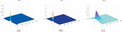
Example 7.1
We select the surplus parameters ,
and
.
By calculating we have . Model (Equation2
(2)
(2) ) has disease-free equilibrium
. We give the initial value of solution
as follows:
,
and
. The numerical simulations in Figure elucidate that equilibrium
is globally asymptotically stable. Thus, the open problem in Remark 4 is verified to may be right.
Figure 1. Dynamical behaviours of (a),
(b) and
(c). The numerical simulations indicate that the solutions finally converge to equilibrium
.
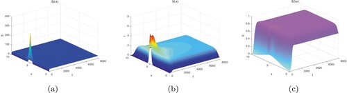
Example 7.2
We choose the surplus parameters ,
and
.
By calculating we have . We give the initial value of solution
as follows:
,
and
. The numerical simulations in Figure elucidate that equilibrium
is globally asymptotically stable. Thus, the open problem in Remark 8 is verified to may be right.
Figure 2. Dynamical behaviours of (a),
(b) and
(c). The numerical simulations indicate that the solutions finally converge to equilibrium
.
8. Conclusion
In this paper, we propose a reaction-diffusion SIR model via environmental driven infection in heterogeneous space. In addition, the model also includes the protective measures taken by humans in response to the infectious disease. For example, the susceptible wear masks, isolation and treatment for the infected. The above methods block human to human transmission, but it also complicates the spread of the epidemic. It is clear that the nonlinear incidence rate is more suitable for the situation after the implementation of the above measures (see [Citation17, Citation18, Citation26, Citation28, Citation36, Citation40]). Therefore, it is of practical significance to study the threshold dynamics of the epidemic with nonlinear incidence.
Firstly, the well-posedness of solutions is obtained. Secondly, the basic reproduction number is calculated. Thirdly, we establish a threshold condition for the global asymptotic stability of disease-free equilibrium
by applying the theory of asymptotically autonomous semiflows and the Lyapunov function theory, respectively. In terms of epidemiology, when
, the number of the infected and the content of pathogens in the environment will gradually become zero, and eventually the epidemic becomes extinct. On the contrary, when
we get the uniform persistence of model (Equation2
(2)
(2) ) by adopting the persistence theory of dynamical systems, and model (2) has at least one endemic equilibrium. Furthermore, when
, the global asymptotic stability of endemic equilibrium
is obtained in the spatially homogenous case. That is, when
although many infected people are cured in the hospital, newly infected individuals will continue to appear so that the number of infected people and the content of pathogens in the environment remain at a high level. Therefore, the epidemic will continue to spread and pose a serious impact on human health.
However, it is a pity that we don't acquire the global asymptotic stability of disease-free equilibrium when
and the global asymptotic stability of endemic equilibrium
when
. Therefore, we propose an open question in Remarks 4 and 8, respectively, and verify those problems by numerical examples. As for the theoretical results of the above two questions, we will study and solve them in the future.
In this paper, we think that after the implementation of the prevention and control measures of the epidemic, the transmission route of human to human has been cut off, and environment-driven infection has become the only transmission route of the epidemic. However, in the actual process of epidemic prevention and control, human to human transmission and environment-driven infection always coexist, and it is difficult to completely prevent human to human transmission of the epidemic. Therefore, in order to make the model more realistic, we propose an epidemic model with two transmission routes.
Furthermore, if we consider the epidemic with latent period and the isolation of asymptomatic infectors and close contacts, we can establish a kind of epidemic dynamics model with reaction-diffusion and environmental pathogens infection, including susceptible class, latent class, infected class, asymptomatic infection class, isolated class, and environmental pathogens. The above model can more accurately describe the actual situation of the spread of the epidemic, so we must make a detailed theoretical analysis and numerical simulation of the model. We believe that the results will have very important practical significance.
Also, we know that since people learn about the spread of the epidemic through media reports or other channels, they will make corresponding behavioural changes based on the received information. In response to this phenomenon, some researchers have introduced the effects of human memory and learning behaviours on epidemic transmission into epidemic models (see [Citation11]), which makes epidemic models more realistic and results of the study more meaningful. Reaction-diffusion epidemic models that take human memory and learning behaviour into account will be a very interesting research topic. We hope to investigate this in the future.
Acknowledgments
We would like to thank the anonymous referees for their helpful comments and the editor for his constructive suggestions, which greatly improved the presentation of this paper.
Disclosure statement
No potential conflict of interest was reported by the author(s).
Additional information
Funding
References
- E.S. Amirian, Potential fecal transmission of SARS-CoV-2: Current evidence and implications for public health, Int. J. Infect. Dis. 95 (2020), pp. 363–370.
- A.A.M. Arafa, S.Z Rida, and M. Khalil, Fractional modeling dynamics of HIV and CD4+ T-cells during primary infection, Nonlinear Biomed. Phys. 6 (2012), p. 1.
- A.A.M. Arafa, M. Khalil, and A. Sayed, A non-integer variable order mathematical model of human immunodeficiency virus and malaria coinfection with time delay, Complexity 2019 (2019), p. 4291017.
- M. Arslan, B. Xu, and M.G. El-Din, Transmission of SARS-CoV-2 via fecal-oral and aerosols-borne routes: Environmental dynamics and implications for wastewater management in underprivileged societies, Sci. Total Environ. 743 (2020), p. 140709.
- Z. Bai, R. Peng, and X. Zhao, A reaction-diffusion malaria model with seasonality and incubation period, J. Math. Biol. 77 (2018), pp. 201–228.
- F. Capone, V.D. Cataldis, and R.D. Luca, Influence of diffusion on the stability of equilibria in a reaction-diffusion system modeling cholera dynamic, J. Math. Biol. 71 (2015), pp. 1107–1131.
- C. Chuah, G.N. Gobert, B. Latif, C.C. Heo, and C.Y. Leow, Schistosomiasis in Malaysia: A review, Acta Trop. 190 (2019), pp. 137–143.
- T. Chen, J. Rui, Q. Wang, Z. Zhao, J. Cui, and L. Yin, A mathematical model for simulating the transmission of Wuhan novel coronavirus, bioRxiv (2020), p. 911669. Available at http://dx.doi.org/10.1101/2020.01.19.911669.
- J.G.B. Derraik and D. Slaney, Anthropogenic environmental change, mosquito-borne diseases and human health in New Zealand, Ecohealth 4 (2007), pp. 72–81.
- J. Deen, M.A. Mengel, and J.D. Clemens, Epidemiology of cholera, Vaccine 38 (2020), pp. A31–A40.
- A.M.A. El-Sayed, A.A.M. Arafa, M. Khalil, and A. Sayed, Backward bifurcation in a fractional order epidemiological model, Progr. Fract. Differ. Appl. 3 (2017), pp. 281–287.
- Z. Feng, J.X. Velasco-Hernandez, B. Tapia-Santos, and M.C.A. Leite, A model for coupling within-host and between-host dynamics in an infectious disease, Nonlinear Dyn. 68 (2012), pp. 401–411.
- Z. Feng, J.X. Velasco-Hernandez, and B. Tapia-Santos, A mathematical model for coupling within-host and between-host dynamics in an environmentally infectious disease, Math. Biosci. 241 (2013), pp. 49–55.
- Z. Feng, X. Cen, Y. Zhao, and J.X. Velasco-Hernandez, Coupled within-host and between-host dynamics and evolution of virulence, Math. Biosci. 270 (2015), pp. 204–212.
- J. Groeger, Divergence theorems and the supersphere, J. Geom. Phys. 77 (2014), pp. 13–29.
- R. Gupta and A.K. Misra, Drinking water quality problem in Haryana, India: Prediction of human health risks, economic burden and assessment of possible intervention options, Environ. Dev. Sustain21 (2019), pp. 2097–2111.
- P. Georgescu and H. Zhang, A Lyapunov functional for an SIRI model with nonlinear incidence of infection and relapse, Appl. Math. Comput. 219 (2013), pp. 8496–8507.
- S. Gao, L. Chen, J.J. Nieto, and A. Torres, Analysis of a delayed epidemic model with pulse vaccination and saturation incidence, Vaccine 24 (2006), pp. 6037–6045.
- K.A.M. Gaythorpe, C.L. Trotter, and A.J.K. Conlan, Modelling norovirus transmission and vaccination, Vaccine 36 (2018), pp. 5565–5571.
- M. Gallo, L. Ferrara, A. Calogero, D. Montesano, and D. Naviglio, Relationships between food and diseases: What to know to ensure food safety, Food Res. Int. 137 (2020), pp. 109414.
- J.K. Hale, Asymptotic Behavior of Dissipative Systems, American Mathematical Society, Providence, RI, 1988.
- S. Inaida, Y. Shobugawa, S. Matsuno, R. Saito, and H. Suzuki, The spatial diffusion of norovirus epidemics over three seasons in Tokyo, Epidemiol. Infect. 143 (2015), pp. 522–528.
- T. Kuniya and J. Wang, Global dynamics of an SIR epidemic model with nonlocal diffusion, Nonlinear Anal. RWA 43 (2018), pp. 262–282.
- H. Lin and F. Wang, Global dynamics of a nonlocal reaction-diffusion system modeling the West Nile virus transmission, Nonlinear Anal. RWA 46 (2019), pp. 352–373.
- Y. Lou and X. Zhao, A reaction-diffusion malaria model with incubation period in the vector population, J. Math. Biol. 62 (2011), pp. 543–568.
- J. Li, Y. Yang, Y. Xiao, and S. Liu, A class of Lyapunov functions and the global stability of some epidemic models with nonlinear incidence, J. Appl. Anal. Comput. 6 (2016), pp. 38–46.
- Q. Liu, D. Jiang, T. Hayat, and A. Alsaedi, Dynamical behavior of a stochastic epidemic model for cholera, J. Franklin Inst. 356 (2019), pp. 7486–7514.
- Y. Luo, L. Zhang, T. Zheng, and Z. Teng, Analysis of a diffusive virus infection model with humoral immunity cell-to-cell transmission and nonlinear incidence, Physica A 535 (2019), p. 122415.
- J. Lu, Z. Teng, and Y. Li, An age-structured model for coupling within-host and between-host dynamics in environmentally-driven infectious diseases, Chaos Solit. Fract. 139 (2020), p. 110024.
- Y. Luo, L. Zhang, Z. Teng, and T. Zheng, Analysis of a general multi-group reaction-diffusion epidemic model with nonlinear incidence and temporary acquired immunity, Math. Comput. Simul. 182 (2021), pp. 428–455.
- R.E. Mickens, Nonstandard finite difference schemes for reaction-diffusion equations, Numer. Methods Part. D. E 15 (1999), pp. 201–214.
- R.E. Mickens, Dynamics consistency: A fundamental principle for constructing nonstandard finite difference scheme for differential equation, J. Differ. Equ. Appl. 11 (2005), pp. 645–653.
- R.E. Mickens, Numerical integration of population models satisfying conservation laws: NSFD methods, J. Biol. Dyn. 1 (2007), pp. 427–436.
- C.L. Moe, Preventing norovirus transmission: How should we handle food handlers?, Clin. Infect. Dis.48 (2009), pp. 38–40.
- R.H Martin and H.L. Smith, Abstract functional differential equations and reaction-diffusion systems, Trans. Am. Math. Soc. 321 (1990), pp. 1–44.
- H. Miao, Z. Teng, and X. Abdurahman, Stability and Hopf bifurcation for a five-dimensional virus infection model with Beddington-DeAngelis incidence and three delays, J. Biol. Dyn. 12 (2018), pp. 146–170.
- M. Park, Infectious disease-related laws: Prevention and control measures, Epidemiol. Health. 39 (2017), p. e2017033.
- M.H. Protter and H.F. Weinberger, Maximum Principles in Differential Equations, Prentice Hall, Englewood Cliffs, 1967.
- S. Palani, M. Nagarajan, A.K. Biswas, R. Reesu, and V. Paluru, Hand, foot and mouth disease in the Andaman Islands, India, Indian Pediat. 55 (2018), pp. 408–410.
- S. Ruan and W. Wang, Dynamical behavior of an epidemic model with a nonlinear incidence rate, J. Differ. Equ. 188 (2003), pp. 135–163.
- H.L. Smith, Monotone Dynamical Systems: An Introduction To the Theory of Competitive and Cooperative Systems, American Mathematical Society, Providence, RI, 1995.
- H.L. Smith and X. Zhao, Robust persistence for semidynamical systems, Nonlinear Anal. 47 (2001), pp. 6169–6179.
- H.R. Thieme, Convergence results and a Poincare-Bendixson trichoyomy for asymptotically autonomous differential equations, J. Math. Biol. 30 (1992), pp. 755–763.
- W. Wang and X. Zhao, Basic reproduction numbers for reaction-diffusion epidemic models, SIAM J. Appl. Dyn. Syst. 11 (2012), pp. 1652–1673.
- Y. Wu and X. Zou, Dynamics and profiles of a diffusive host-pathogen system with distinct dispersal rates, J. Differ. Equ. 264 (2018), pp. 4989–5024.
- Q. Ye, Z. Li, M. Wang, and Y. Wu, Introduction to Reaction-Diffusion Equations (In Chinese), 2nd ed., Science Press, Beijing, 2011.
- J. Yang, R. Xu, and J. Li, Threshold dynamics of an age-space structured brucellosis disease model with Neumann boundary condition, Nonlinear Anal. RWA 50 (2019), pp. 192–217.
- J. Yang, R. Xu, and H. Sun, Dynamics of a seasonal brucellosis disease model with nonlocal transmission and spatial diffusion, Commun. Nonlinear Sci. Numer. Simul. 94 (2021), p. 105551.