Building mean field ODE models using the generalized linear chain trick & Markov chain theory

ABSTRACT

The well known linear chain trick (LCT) allows modellers to derive mean field ODEs that assume gamma (Erlang) distributed passage times, by transitioning individuals sequentially through a chain of sub-states. The time spent in these sub-states is the sum of k exponentially distributed random variables, and is thus gamma distributed. The generalized linear chain trick (GLCT) extends this technique to the broader phase-type family of distributions, which includes exponential, Erlang, hypoexponential, and Coxian distributions. Phase-type distributions are the family of matrix exponential distributions on $[0,\mathrm{\infty })$ that represent the absorption time distributions for finite-state, continuous time Markov chains (CTMCs). Here we review CTMCs and phase-type distributions, then illustrate how to use the GLCT to efficiently build ODE models from underlying stochastic model assumptions. We introduce two novel model families by using the GLCT to generalize the Rosenzweig-MacArthur predator-prey model, and the SEIR model. We illustrate the kinds of complexity that can be captured by such models through multiple examples. We also show the benefits of using a GLCT-based model formulation to speed up the computation of numerical solutions to such models. These results highlight the intuitive nature, and utility, of using the GLCT to derive ODE models from first principles.

Keywords:

• Linear chain trick
• gamma chain trick
• phase-type distribution
• Coxian distribution
• Erlang distribution

1. Introduction

Continuous time state transition models, often formulated as mean field ODE models, are widely used throughout the biological sciences and across multiple scales [4,9,13,25,30,31,39,53,56,57,78,79,82,103,111]. Examples include models of multi-species interactions [76,81], infectious disease transmission [7,28,35,71], cell proliferation and cancer [18,26,43,65,98,113], and various other applications in which entities transition among a finite number of states. One criticism of mean field ODE models is that they often implicitly assume that the time individuals spend in the different states are exponentially distributed [36,110]. That is, an ODE model with a linear loss rate can be interpreted as implicitly assuming an underlying stochastic state transmission model with an exponentially distributed dwell-time in the focal state. For example, the simple model $\mathrm{d}x/\mathrm{d}t=b-\mathrm{d}x$ is consistent with assuming an underlying stochastic state transition model in which individuals spend an exponentially distributed amount of time with mean 1/d in the state corresponding to variable x.

Importantly, the timing of state transitions can meaningfully affect model dynamics and model outputs in an applied setting [67,68,79,80,84,96,110]. One remedy to address this issue with ODE models is known as the linear chain trick (LCT) [22,23,33,51,68–70,73,100,107,108], which allows modellers to instead assume gamma (Erlang¹) distributed passage times (a.k.a., dwell times). This is accomplished by partitioning a state into a series of k sub-states, where individuals transition sequentially through this ‘linear chain’ of sub-states. The resulting time spent in this collection of sub-states is thus the sum of k exponentially distributed random variables, and therefore follows an Erlang distribution (if the each exponential has the same rate) or a generalized Erlang² distribution (if the rates differ).

The generalized linear chain trick (GLCT) [51] extends this technique to allow modellers to assume these passage times follow a much broader family of distributions that includes the phase-type family of distributions [15,44,46,66,91]. These real-valued, matrix exponential distributions on $[0,\mathrm{\infty })$ are the family of all possible hitting time (or absorption time) distributions for finite-state, absorbing, continuous time Markov chains (CTMCs). See Equations (4(4c) $\begin{array}{rl}E(Y^j)& =j!{\mathit{\alpha }}^{\mathbf{T}}(-\mathbf{A}{)}^{-j}\mathbf{1}.\end{array}$(4c) ) in Section 1.1.2 below for a more detailed definition, and for further details, see [5,15,44–46,91,92,102]. This broad family includes exponential, Erlang, hypoexponential, hyperexponential, and Coxian distributions [15,38,46,91]. The phase-type family is also closed under various operations including minimum, finite mixtures, and convolutions (sums) [14]. Recently, phase-type distributions have been increasingly applied outside of queuing theory, where much of the theory and methods for phase-type distributions have been developed [10,46,75,77,89]. For example, they are increasingly being used in biology and medicine [1,32,40,74,104]. Importantly, the availability of statistical tools for estimating such distributions from data has been increasing (e.g.[44–47]), allowing researchers to build approximate empirical distributions into ODE models using the GLCT.

In this article, we build upon the theoretical foundation laid out in [51] and illustrate how to use the GLCT, in conjunction with concepts and techniques from CTMC theory, to build mean field ODE models using a much richer set of possible underlying stochastic model assumptions. We also demonstrate the potential computational benefits of using GLCT-based model formulations. The paper is organized as follows: First, we review CTMCs, phase-type distributions, and then the GLCT for phase-type distributions. Then, we generalize some simple biological state transition models by replacing their implicit assumption of exponentially distributed passage time assumptions with arbitrary phase-type distributions. We also illustrate how to implement a sub-state transition that does not affect the overall distribution of time spent in that state using the example of hospitalization without altering the infectious period distribution. Lastly, we investigate some of the costs and benefits of using this generalized model framework with regards to computing numerical solutions. These results highlight the efficient, intuitive nature of using this novel approach to derive mean field state transition models from explicitly stochastic assumptions framed in the context of Poisson processes and CTMCs.

1.1. Continuous time Markov chains & phase-type distributions

To provide proper context for an intuitive understanding of the generalized linear chain trick (GLCT), we briefly review continuous time Markov chains (CTMCs) with a focus on CTMCs that have a single absorbing state. Our focus will then be on the probability distributions that describe the time it takes to reach that absorbing state starting from one of the transient states. These absorption time distributions define the phase-type family of distributions [15,46,66,91]. The summaries below build upon the similar descriptions laid out in [51].

1.1.1. Discrete & continuous time Markov chains

Discrete time Markov chains (DTMCs) describe the transition of an individual (or other distinct entity) among a set of n states [11,48,94,102]. For our purposes below, we will restrict our attention to Markov chains in which the first k = n−1 states are transient states and the last $(k+1)$ state is an absorbing state. That is, eventually, the system enters this last state and remains there on each subsequent time step with probability 1. The initial-state distribution vector is $[{\alpha }_1,\dots ,{\alpha }_k,{\alpha }_{\ast }{]}^{\mathrm{T}}$ where each value is non-negative and ${\alpha }_{\ast }+\sum _{i=1}^k{\alpha }_i=1$. We will refer to the transient states component of this initial distribution vector with column vector $\mathit{\alpha }=[{\alpha }_1,\dots ,{\alpha }_k{]}^{\mathrm{T}}$. The transition probabilities from the ith state to the jth state ($p_{ij}$ where $1\le i,j\le n$) are best organized using a transition probability matrix $\mathbf{P}$, where $p_{ij}$ is value in the ith row and jth column of the matrix ($P_{ij}=p_{ij}$).

The transition probability matrix $\mathbf{P}$ can be written in block form [11,94] according to these first k = n−1 transient states (we'll call this set of states X) and the last absorbing state as (1) $\mathbf{P}=\left[\begin{array}{cc}{\mathbf{P}}_{\mathbf{X}}& {\mathbf{P}}_{\mathbf{a}}\\ \mathbf{0}& 1\end{array}\right]$(1) where ${\mathbf{P}}_{\mathbf{X}}$ is a $k\times k$ matrix describing transition probabilities among transient states, ${\mathbf{P}}_{\mathbf{a}}$ is the $k\times 1$ vector of probabilities of transitioning from the ith transient state to the absorbing state, and $\mathbf{0}$ is a $1\times k$ vector of zeros.

In a continuous time Markov chain (CTMC), these transitions don't occur according to a fixed time step, but instead each transition occurs after an exponentially distributed amount of time [11,48,94,102]. If the individual is in the ith state, that exponential distribution has rate ${\lambda }_i$ or equivalently has mean duration $1/{\lambda }_i$. Let $\mathbf{R}$ be the vector of these rates ${\lambda }_i$, $i=1,\dots ,k$. Due to the memorylessness property of exponential distributions, transitions from state i to state i can effectively be ignored, thus we can formulate a new transition probability matrix that describes an equivalent Markov chain but where we only track transitions to new states. This reformulated Markov chain is known as the embedded jump process or embedded Markov chain [48], and it is described with a transition probability matrix $\stackrel{\mathbf{~}}{\mathbf{P}}$ where the diagonal entries are 0, and the off diagonal transition probabilities ${\tilde{p}}_{ij}=p_{ij}/\sum _{j\ne i}{p}_{ij}$. That is, these are just the off-diagonal entries of $\mathbf{P}$ with the diagonal set to 0, and the rows normalized so each row sums to 1. For our purposes, since a Markov chain with an absorbing state is not ergodic and therefore does not properly have an embedded jump process representation, the above procedure is only applied to k rows corresponding to transient states. Hence, the last row of $\mathbf{P}$ and $\stackrel{\mathbf{~}}{\mathbf{P}}$ will be the same, so that the last state in the Markov chain remains an absorbing state.

In a CTMC context, the transition probability matrix $\stackrel{\mathbf{~}}{\mathbf{P}}$ and rate vector $\mathbf{R}$ are usually combined into a single matrix called the transition rate matrix $\mathbf{Q}$ [48,99]. The entries of $\mathbf{Q}$ can be thought of as the mean-field, per-individual loss rates from each state (along the diagonal) and the transition rates from the ith state into the jth state (the off diagonal entries). It has the block form (2) $\mathbf{Q}=\left[\begin{array}{cc}\mathbf{A}& \mathbf{B}\\ \mathbf{0}& 0\end{array}\right]$(2) where $\mathbf{A}$ is a $k\times k$ matrix describing the transition rates among transient states, $\mathbf{B}$ is the $k\times 1$ vector of transition rates from the transient states to the absorbing state, and the bottom row is all zeros for the absorbing state.

Matrices $\mathbf{A}$ and $\mathbf{B}$ are constructed from the entries of the transition probability matrix $\stackrel{\mathbf{~}}{\mathbf{P}}$ and the vector of rates for the exponential distributed dwell-times $\mathbf{R}$ as follows. The ith diagonal entry of $\mathbf{A}$ is the loss rate $-{\lambda }_i$ and the rest of the entries in the ith row are the product of the ${\lambda }_i$ and the transition probabilities ${\tilde{p}}_{ij}$. That is, the ij off-diagonal entries of $\mathbf{A}$ are the per-individual transition rates from the ith state into the jth state, given by ${\lambda }_i{\tilde{p}}_{ij}$. Since the rows of $\stackrel{\mathbf{~}}{\mathbf{P}}$ sum to 1, the rows of $\mathbf{Q}$ sum to 0, and it then follows that vector $\mathbf{B}$ is equal to the negative of the row sums of $\mathbf{A}$. Thus, one can write $\mathbf{B}=-\mathbf{A}\mathbf{1}$, where $\mathbf{1}$ is a column vector of k ones.

The above shows that, for CTMCs which have k transient states and 1 absorbing state, all of the information necessary to describe the CTMC is contained in the transition rate matrix for transient states, $\mathbf{A}$, and initial distribution vector $\mathit{\alpha }$. As detailed next, these two quantities are also sufficient to parameterize the phase-type distribution corresponding to such a CTMC.

1.1.2. Phase-type distributions

With the above family of CTMCs in mind, let $Y_i$ be defined as the duration of time that it takes to first reach the absorbing state, given the CTMC starts in the ith transient state. We call this an absorption time [94]. More generally, let Y be the absorption time where the initial state is determined by the initial probability vector $\mathit{\alpha }$ (i.e. Y follows the mixture distribution of random variables $Y_i$ with mixing probabilities $\mathit{\alpha }$).

Phase-type distributions are the family of absorption time distributions for all such Y described above. The most familiar examples are perhaps the exponential distributions and the Erlang distributions, i.e. those gamma distributions that have an integer shape parameter, k, and can therefore be thought of as the sum of k independent exponentially distributed random variables, each with rate r. Erlang distributions can be parameterized in terms of their mean μ and variance ${\sigma }^2$ (or coefficient of variation $c_v$, the standard deviation over the mean), or parameters rate r and shape k, where (3) $\mu =\frac{k}{r},{\sigma }^2=\frac{k}{r^2},c_v=\frac{1}{\sqrt{k}},\mathrm{and}\mathrm{thus},r=\frac{\mu }{{\sigma }^2},\mathrm{and}k=\frac{{\mu }^2}{{\sigma }^2}=\frac{1}{c_v^2}.$(3) More generally, as detailed in [15,91], phase-type distributions are parameterized by vector $\mathit{\alpha }$ and transient state rate matrix $\mathbf{A}$, and have the probability density function $f(t)$, cumulative density function $F(t)$, and jth moment function $E(Y^j)$ given by: (4a) $\begin{array}{rl}f(t)& ={\mathit{\alpha }}^{\mathbf{T}}{e}^{\mathbf{A}t}(-\mathbf{A}\mathbf{1})\end{array}$(4a) (4b) $\begin{array}{rl}F(t)& =1-{\mathit{\alpha }}^{\mathbf{T}}{e}^{\mathbf{A}t}\mathbf{1}\end{array}$(4b) (4c) $\begin{array}{rl}E(Y^j)& =j!{\mathit{\alpha }}^{\mathbf{T}}(-\mathbf{A}{)}^{-j}\mathbf{1}.\end{array}$(4c) Here $\mathbf{1}$ is a column vector of ones with the same number of rows as $\mathit{\alpha }$ and $\mathbf{A}$. Note that $\mathit{\alpha }$ and $\mathbf{A}$ are not necessarily a unique parameterization of a given phase-type distribution, as there are often equivalent parameterizations using vector-matrix pairs of the same dimension as well as different dimensions [85,95]. Phase-type distributions can be classified as cyclic (transient states can be visited infinitely often) and acyclic (transient states can only be visited once), and all acyclic phase-type distributions have a Coxian representation [21,27,85]. This family of distributions has been relatively well studied in the queuing theory literature, and for further details, readers are encouraged to consult [5,14,15,44,45,85–87,91,92] and related works.

Additionally, freely available computational tools such as BuTools for Matlab and Python [46,47] enable researchers to fit phase-type distributions to data or to approximate other distributions (see also [66]). This fact, combined with the GLCT, allows for the construction of ODE models that incorporate empirically derived (or other) distributional assumptions for the time spent in a given state.

1.2. Generalized linear chain trick

The GLCT provides modellers with a direct way to use the matrix and vector parameterization of a given phase-type distribution to take an existing ODE model with exponentially distributed dwell times, and replace the ODE equation for that state by a set of ODEs that describe a set of sub-states that together incorporate an overall dwell-time distribution that obeys the given phase-type distribution [49,51]. This technique can also be used to implement the classic linear chain trick (LCT), as Erlang distributions are a subfamily of phase-type distributions.

The GLCT in its most general form [51] extends the GLCT for phase-type distributions to the scenario where the rates and probabilities in the CTMC framework described above can vary with time. Here, we only provide a statement of the GLCT for phase-type distributions:

Theorem 1.1

GLCT for phase-type distributions [Corollary 2 in [51]

] Assume individuals enter state X at rate $\mathcal{I}(t)$ and that the distribution of time spent in state X follows a continuous phase-type distribution given by the $k\times 1$ initial probability vector $\mathit{\alpha }$ and the $k\times k$ matrix $\mathbf{A}$, where k is a positive integer. Then state X can be partitioned into k sub-states and the mean field equations for the amounts in each sub-state at time t, $x_i(t),$ are given by (5) $\frac{\mathrm{d}}{\mathrm{d}t}\mathbf{x}(t)=\mathit{\alpha }\mathcal{I}(t)+{\mathbf{A}}^{\mathrm{T}}\mathbf{x}(t)$(5) where $\mathbf{x}(t)=[x_1(t),\dots ,x_k(t){]}^{\mathrm{T}}$, the rate of individuals leaving each of these sub-states of X is given by the vector $(-\mathbf{A}\mathbf{1})\circ \mathbf{x}(t),$ where ° is the Hadamard (element-wise) product of the two vectors, and thus the total rate of individuals leaving state X is given by the sum of those terms, i.e.$(-\mathbf{A}\mathbf{1}{)}^{\mathrm{T}}\mathbf{x}(t)=-{\mathbf{1}}^{\mathrm{T}}{\mathbf{A}}^{\mathrm{T}}\mathbf{x}(t)$.

Note that, assuming an overall influx rate of $\mathcal{I}(t)$ at time t, this influx is distributed across the sub-states of X according to the initial distribution vector $\mathit{\alpha }$, and the second term in Equation (5(5) $\frac{\mathrm{d}}{\mathrm{d}t}\mathbf{x}(t)=\mathit{\alpha }\mathcal{I}(t)+{\mathbf{A}}^{\mathrm{T}}\mathbf{x}(t)$(5) ) describes both the movements among sub-states of X as well as the loss rate from the state X contributed from each sub-state.

The linear chain trick (LCT) has been known for decades [22,23,33,51,69,70,73,100,107, 108], and is special case of the GLCT for phase-type distributions stated above [51]. For completeness, below we provide a formal statement of the LCT, which assumes an Erlang distributed dwell time with shape k and rate r.

Corollary 1.2

Linear Chain Trick

Consider the GLCT above. Assume that the dwell-time distribution is an Erlang distribution with shape k and rate r $($or if written in terms of shape k and mean $\tau =k/r,$ then use rate $r=k/\tau )$. Then the corresponding mean field ODE equations for the k sub-states of X are (6) $\begin{array}{rl}\frac{\mathrm{d}{x}_1}{\mathrm{d}t}& =\mathcal{I}(t)-r{x}_1\\ \frac{\mathrm{d}{x}_2}{\mathrm{d}t}& =r{x}_1-r{x}_2\\ & ⋮\\ \frac{\mathrm{d}{x}_k}{\mathrm{d}t}& =r{x}_{k-1}-r{x}_k.\end{array}$(6) where the total loss rate from state X at time t is the loss rate from the final sub-state, $r{x}_k(t)$.

Proof.

The phase-type distribution formulation of the Erlang distribution with shape k and rate r is given by v and M below, and substituting these into Equation (5(5) $\frac{\mathrm{d}}{\mathrm{d}t}\mathbf{x}(t)=\mathit{\alpha }\mathcal{I}(t)+{\mathbf{A}}^{\mathrm{T}}\mathbf{x}(t)$(5) ) yields the desired result. (7) $\mathbf{\text{v}}=\left[\begin{array}{c}1\\ 0\\ ⋮\\ 0\end{array}\right]\mathrm{and}\mathbf{\text{M}}=\left[\begin{array}{ccccc}-r& r& 0& \cdots & 0\\ 0& -r& r& \ddots & 0\\ ⋮& \ddots & \ddots & \ddots & \ddots \\ 0& 0& \ddots & -r& r\\ 0& 0& \cdots & 0& -r\end{array}\right]$(7) See [51] for a direct proof that uses a recursive relationship between Erlang density functions and their derivatives.

2. Results

In the sections below, we extend some well-known models using the GLCT by replacing the implicit exponentially distributed dwell time assumptions of these models with phase-type distribution assumptions. Importantly, these more general model formulations can also be used as a way to formulate models derived using the standard LCT (i.e.the assumption of Erlang distributed dwell times), as the phase-type formulation of such models can often be more practically and computationally advantageous to work with, and we show in section 2.4.

2.1. Rosenzweig-MacArthur predator-prey model

Maturation delays in population models can influence model outputs, however, such delays are not always incorporated into models used in applications [96]. In this section, we illustrate how one can use the GLCT to incorporate phase-type maturation times into such population models, using the well known Rosenzweig-MacArthur model of predator-prey (consumer-resource) dynamics [81,97]: (8a) $\begin{array}{rl}\frac{\mathrm{d}N}{\mathrm{d}t}& =rN(1-\frac{N}{K})-\frac{aP}{h+N}N\end{array}$(8a) (8b) $\begin{array}{rl}\frac{\mathrm{d}P}{\mathrm{d}t}& =\chi \frac{aN}{h+N}P-\mu P\end{array}$(8b)

In the absence of predators (P), the prey population (N) is subject to logistic growth, and predators consume prey following a Holling's type II functional response [24,41,42,81]. Predators live for an exponentially distributed lifetime with mean $1/\mu$.

One can incorporate a maturation delay of duration τ by formulating a delay differential equation (DDE) extension of Equation (8(8b) $\begin{array}{rl}\frac{\mathrm{d}P}{\mathrm{d}t}& =\chi \frac{aN}{h+N}P-\mu P\end{array}$(8b) ), as in [112]: (9a) $\begin{array}{rl}\frac{\mathrm{d}N(t)}{\mathrm{d}t}& =rN(t)(1-\frac{N(t)}{K})-\frac{aP(t)}{h+N(t)}N(t)\end{array}$(9a) (9b) $\begin{array}{rl}\frac{\mathrm{d}P(t)}{\mathrm{d}t}& =\chi \frac{aN(t-\tau )}{h+N(t-\tau )}P(t-\tau )-\mu P(t)\end{array}$(9b)

This can be thought of as the limit of a distributed delay model, with mean delay time τ, for which the variance (or coefficient of variation) goes to zero to yield a delay distribution with point mass at τ (i.e. the distribution can be described with a Dirac delta function). The LCT has long been used to approximate such limiting cases in DDE models by assuming instead a delay distribution that is Erlang distributed with mean τ and a very small coefficient of variation (small variance), i.e. a large shape parameter $k=1/c_v^2$ [51,100]. Writing this approximating model, as in [50], yields the Rosenzweig–MacArthur model with Erlang distributed maturation time in the predators: (10a) $\begin{array}{rl}\frac{\mathrm{d}N}{\mathrm{d}t}& =rN(1-\frac{N}{K})-\frac{aP}{h+N}N\end{array}$(10a) (10b) $\begin{array}{rl}\frac{\mathrm{d}{x}_1}{\mathrm{d}t}& =\chi \frac{aN}{h+N}P-\frac{k}{\tau }{x}_1\end{array}$(10b) (10c) $\begin{array}{rl}\frac{\mathrm{d}{x}_j}{\mathrm{d}t}& =\frac{k}{\tau }{x}_{j-1}-\frac{k}{\tau }{x}_j,\mathrm{for}j=2,\dots ,k\end{array}$(10c) (10d) $\begin{array}{rl}\frac{\mathrm{d}P}{\mathrm{d}t}& =\frac{k}{\tau }{x}_k-\mu P\end{array}$(10d)

The sub-states $x_i$, $i=1,\dots ,k$, track the immature stages of the predators before they reach maturity.

Using the GLCT [49,51], the above model can be generalized in two ways. First, the Erlang distributed maturation time assumption that yields the sub-states $x_i$ can be replaced by the assumption of a more general phase-type distribution with matrix-vector parameterization ${\mathit{\alpha }}_{\mathbf{X}}$ and ${\mathbf{A}}_{\mathbf{X}}$. Similarly, the exponentially distributed time duration that predators spend as adults can also be replaced with a more general phase-type distribution with parameter vector ${\mathit{\alpha }}_{\mathbf{P}}$ and matrix ${\mathbf{A}}_{\mathbf{P}}$. According to the GLCT, these assumptions yield the more general model (11a) $\begin{array}{rl}\frac{\mathrm{d}N}{\mathrm{d}t}& =rN(1-\frac{N}{K})-\frac{aP}{h+N}N\end{array}$(11a) (11b) $\begin{array}{rl}\frac{\mathrm{d}\mathbf{x}}{\mathrm{d}t}& =\chi \frac{aN}{h+N}P{\mathit{\alpha }}_{\mathbf{X}}+{{\mathbf{A}}_{\mathbf{X}}}^{\mathrm{T}}\mathbf{x}\end{array}$(11b) (11c) $\begin{array}{rl}\frac{\mathrm{d}\mathbf{y}}{\mathrm{d}t}& =\underset{\mathrm{scalar}}{\underbrace{-{\mathbf{1}}^{\mathrm{T}}{{\mathbf{A}}_{\mathbf{X}}}^{\mathrm{T}}\mathbf{x}}}{\mathit{\alpha }}_{\mathbf{P}}+{{\mathbf{A}}_{\mathbf{P}}}^{\mathrm{T}}\mathbf{y}\end{array}$(11c) where $\mathbf{x}(t)$ denotes the vector of maturing predator sub-states $x_i(t)$, $\mathbf{y}(t)$ is the vector of adult predator sub-states $y_j(t)$, and where $P(t)=\sum _{\mathrm{all}j}{y}_j(t)$.

Observe that Equations (10(10d) $\begin{array}{rl}\frac{\mathrm{d}P}{\mathrm{d}t}& =\frac{k}{\tau }{x}_k-\mu P\end{array}$(10d) ) are the special case of Equations (11(11c) $\begin{array}{rl}\frac{\mathrm{d}\mathbf{y}}{\mathrm{d}t}& =\underset{\mathrm{scalar}}{\underbrace{-{\mathbf{1}}^{\mathrm{T}}{{\mathbf{A}}_{\mathbf{X}}}^{\mathrm{T}}\mathbf{x}}}{\mathit{\alpha }}_{\mathbf{P}}+{{\mathbf{A}}_{\mathbf{P}}}^{\mathrm{T}}\mathbf{y}\end{array}$(11c) ) where the phase-type distribution matrix-vector parameterization for an Erlang distribution with mean τ and shape parameter k is given by (12) ${\mathit{\alpha }}_{\mathbf{X}}=\left[\begin{array}{c}1\\ 0\\ ⋮\\ 0\end{array}\right]\mathrm{and}{\mathbf{A}}_{\mathbf{X}}=\left[\begin{array}{cccccc}-\frac{k}{\tau }& \frac{k}{\tau }& 0& 0& \cdots & 0\\ 0& -\frac{k}{\tau }& \frac{k}{\tau }& 0& \cdots & 0\\ & & & \ddots & & \\ 0& 0& 0& \cdots & -\frac{k}{\tau }& \frac{k}{\tau }\\ 0& 0& 0& \cdots & 0& -\frac{k}{\tau }\end{array}\right]$(12) and for an exponential distribution with rate μ, (13) ${\mathit{\alpha }}_{\mathbf{P}}=\left[\begin{array}{c}1\end{array}\right]\mathrm{and}{\mathbf{A}}_{\mathbf{P}}=\left[\begin{array}{c}-\mu \end{array}\right].$(13) Note that Equations (10(10d) $\begin{array}{rl}\frac{\mathrm{d}P}{\mathrm{d}t}& =\frac{k}{\tau }{x}_k-\mu P\end{array}$(10d) ) are a much more compact way of formulating such models without the need to specify the number of sub-states. As will be shown below, this formulation allows modellers to more efficiently write computer code for computing numerical solutions to such models, and also can be used with computer algebra systems generate ODEs like Equations (10(10d) $\begin{array}{rl}\frac{\mathrm{d}P}{\mathrm{d}t}& =\frac{k}{\tau }{x}_k-\mu P\end{array}$(10d) ) from first principles.

2.2. SEIR models

SIR-type models of infectious disease transmission are widely used in the study of infectious diseases, and help inform public health policy and related efforts to limit the spread of infectious diseases [7,17,28,34,35,54,58–63,70,72,109,110]. For example, such models are being used at this time to model the ongoing SARS-CoV-2/COVID-19 pandemic [12,29,83,93].

It is known that including a latent period prior to the onset of symptoms and infectiousness, as well as incorporating non-exponential distributions for the time spent in the different infection states, can be important to include in such models when used in applications [34,69,109,110].

Here we use the GLCT to formulate a more general family of SEIR models, where we assume that the latent period (time spent in state E) and infectious period (time spent in state I) follow independent phase-type distributions. For simplicity, we assume the state variables have been scaled by the total population size so that S + E + I + R = 1, and that there are no births or deaths in the model.

To begin, consider the simple SEIR model below, Equations (14), where S is the fraction of susceptibles in the population, E the fraction of exposed individuals with latent infections, I the fraction of individuals with active infections, and R the fraction of recovered or removed individuals: (14a) $\begin{array}{rl}\frac{\mathrm{d}S}{\mathrm{d}t}& =-\beta SI\end{array}$(14a) (14b) $\begin{array}{rl}\frac{\mathrm{d}E}{\mathrm{d}t}& =\beta SI-r_{E}E\end{array}$(14b) (14c) $\begin{array}{rl}\frac{\mathrm{d}I}{\mathrm{d}t}& =r_{E}E-r_{I}I\end{array}$(14c) (14d) $\begin{array}{rl}\frac{\mathrm{d}R}{\mathrm{d}t}& =r_{I}I\end{array}$(14d)

Next, assume the latent period distribution is phase-type with parameters ${\mathit{\alpha }}_{\mathbf{E}}$ and ${\mathbf{A}}_{\mathbf{E}}$, and the infectious period distribution is also phase-type but with parameters ${\mathit{\alpha }}_{\mathbf{I}}$ and ${\mathbf{A}}_{\mathbf{I}}$. Let $\mathbf{x}=[E_1,\dots {]}^{\mathrm{T}}$ and $\mathbf{y}=[I_1,\dots {]}^{\mathrm{T}}$ be the column vectors of the fraction of individuals in each of the exposed and infectious sub-states, respectively, where $E=\sum E_j$ and $I=\sum I_i$. Then by the GLCT we can write the mean field ODEs for the generalized SEIR model as follows: (15a) $\begin{array}{rl}\frac{\mathrm{d}S}{\mathrm{d}t}& =-\beta SI\end{array}$(15a) (15b) $\begin{array}{rl}\frac{\mathrm{d}\mathbf{x}}{\mathrm{d}t}& ={\mathit{\alpha }}_{\mathbf{E}}\beta SI+{{\mathbf{A}}_{\mathbf{E}}}^{\mathsf{\text{T}}}\mathbf{x}\end{array}$(15b) (15c) $\begin{array}{rl}\frac{\mathrm{d}\mathbf{y}}{\mathrm{d}t}& ={\mathit{\alpha }}_{\mathbf{I}}\underset{\mathrm{scalars}}{\underbrace{((-{\mathbf{A}}_{\mathbf{E}}\mathbf{1}{)}^{\mathsf{\text{T}}}\mathbf{x})}}+{{\mathbf{A}}_{\mathbf{I}}}^{\mathsf{\text{T}}}\mathbf{y}\end{array}$(15c) (15d) $\begin{array}{rl}\frac{\mathrm{d}R}{\mathrm{d}t}& =\overbrace{(-{\mathbf{A}}_{\mathbf{I}}\mathbf{1}{)}^{\mathsf{\text{T}}}\mathbf{y}}\end{array}$(15d)

As in the previous model, to assume (for example) an Erlang distributed latent period with mean ${\tau }_E$ and shape $k_E$, i.e.rate $1/{\tau }_E$ and coefficient of variation $c_v=1/\sqrt{k_E}$, then one would use (16) ${\mathit{\alpha }}_{\mathbf{E}}=\left[\begin{array}{c}1\\ 0\\ ⋮\\ 0\end{array}\right]\mathrm{and}{\mathbf{A}}_{\mathbf{E}}=\left[\begin{array}{cccccc}-\frac{k_E}{{\tau }_E}& \frac{k_E}{{\tau }_E}& 0& 0& \cdots & 0\\ 0& -\frac{k}{{\tau }_E}& \frac{k_E}{{\tau }_E}& 0& \cdots & 0\\ & & & \ddots & & \\ 0& 0& 0& \cdots & -\frac{k_E}{{\tau }_E}& \frac{k_E}{{\tau }_E}\\ 0& 0& 0& \cdots & 0& -\frac{k_E}{{\tau }_E}\end{array}\right].$(16) Similarly, an Erlang infectious period distribution with mean ${\tau }_I$ and shape parameter $k_I$ (coefficient of variation $1/\sqrt{k_I}$) would be parameterized by (17) ${\mathit{\alpha }}_{\mathbf{I}}=\left[\begin{array}{c}1\\ 0\\ ⋮\\ 0\end{array}\right]\mathrm{and}{\mathbf{A}}_{\mathbf{I}}=\left[\begin{array}{cccccc}-\frac{k_I}{{\tau }_I}& \frac{k_I}{{\tau }_I}& 0& 0& \cdots & 0\\ 0& -\frac{k}{{\tau }_I}& \frac{k_I}{{\tau }_I}& 0& \cdots & 0\\ & & & \ddots & & \\ 0& 0& 0& \cdots & -\frac{k_I}{{\tau }_I}& \frac{k_I}{{\tau }_I}\\ 0& 0& 0& \cdots & 0& -\frac{k_I}{{\tau }_I}\end{array}\right].$(17) Simplifying the right hand side of Equations (15(15d) $\begin{array}{rl}\frac{\mathrm{d}R}{\mathrm{d}t}& =\overbrace{(-{\mathbf{A}}_{\mathbf{I}}\mathbf{1}{)}^{\mathsf{\text{T}}}\mathbf{y}}\end{array}$(15d) ) using the matrices and vectors above yields the familiar sub-state equations for an SEIR model with Erlang distributed latent and infectious periods [6,55,69,72,110]: (18a) $\begin{array}{rl}\frac{\mathrm{d}S}{\mathrm{d}t}& =-\beta SI\end{array}$(18a) (18b) $\begin{array}{rl}\frac{\mathrm{d}\mathbf{x}}{\mathrm{d}t}& =\left[\begin{array}{c}\beta SI-\frac{k_E}{{\tau }_E}{E}_1\\ \frac{k_E}{{\tau }_E}{E}_1-\frac{k_E}{{\tau }_E}{E}_2\\ \frac{k_E}{{\tau }_E}{E}_2-\frac{k_E}{{\tau }_E}{E}_3\\ ⋮\\ \frac{k_E}{{\tau }_E}{E}_{k_E-1}-\frac{k_E}{{\tau }_E}{E}_{k_E}\end{array}\right]\end{array}$(18b) (18c) $\begin{array}{rl}\frac{\mathrm{d}\mathbf{y}}{\mathrm{d}t}& =\left[\begin{array}{c}\frac{k_E}{{\tau }_E}{E}_{k_E}-\frac{k_I}{{\tau }_I}{I}_1\\ \frac{k_I}{{\tau }_I}{I}_1-\frac{k_I}{{\tau }_I}{I}_2\\ \frac{k_I}{{\tau }_I}{I}_2-\frac{k_I}{{\tau }_I}{I}_3\\ ⋮\\ \frac{k_I}{{\tau }_I}{I}_{k_I-1}-\frac{k_I}{{\tau }_I}{I}_{k_I}\end{array}\right]\end{array}$(18c) (18d) $\begin{array}{rl}\frac{\mathrm{d}R}{\mathrm{d}t}& =\frac{k_I}{{\tau }_I}{I}_{k_I}\end{array}$(18d) where $\mathbf{x}=[E_1,\dots ,E_{k_E}{]}^{\mathrm{T}}$, $\mathbf{y}=[I_1,\dots ,I_{k_I}{]}^{\mathrm{T}}$, and $I=\sum I_i$. By allowing different loss rates from each substate in Equation (15(15d) $\begin{array}{rl}\frac{\mathrm{d}R}{\mathrm{d}t}& =\overbrace{(-{\mathbf{A}}_{\mathbf{I}}\mathbf{1}{)}^{\mathsf{\text{T}}}\mathbf{y}}\end{array}$(15d) ) (i.e. in each row of the matrix in Equation (16(16) ${\mathit{\alpha }}_{\mathbf{E}}=\left[\begin{array}{c}1\\ 0\\ ⋮\\ 0\end{array}\right]\mathrm{and}{\mathbf{A}}_{\mathbf{E}}=\left[\begin{array}{cccccc}-\frac{k_E}{{\tau }_E}& \frac{k_E}{{\tau }_E}& 0& 0& \cdots & 0\\ 0& -\frac{k}{{\tau }_E}& \frac{k_E}{{\tau }_E}& 0& \cdots & 0\\ & & & \ddots & & \\ 0& 0& 0& \cdots & -\frac{k_E}{{\tau }_E}& \frac{k_E}{{\tau }_E}\\ 0& 0& 0& \cdots & 0& -\frac{k_E}{{\tau }_E}\end{array}\right].$(16) )) one could similarly implement a generalized Erlang (or hypoexponential) distribution.

Other phase-type distributions can also be implemented using Equations (15(15d) $\begin{array}{rl}\frac{\mathrm{d}R}{\mathrm{d}t}& =\overbrace{(-{\mathbf{A}}_{\mathbf{I}}\mathbf{1}{)}^{\mathsf{\text{T}}}\mathbf{y}}\end{array}$(15d) ). For example, consider the Coxian distribution [19,20,37,38,74,75,95,104], which is a further generalization of the generalized Erlang distribution. These also have potentially distinct loss rates from each of the k sub-states, plus an additional k−1 proportions (${\rho }_i$) that describe the fraction of those transitions leaving the ith state that go to the i + 1 state. The remaining fraction ($1-{\rho }_i$) go directly to the absorbing state (i.e. if all ${\rho }_i=1$ the Coxian distribution simplifies to a generalized Erlang distribution).

In [64], an SEIR model with a Coxian latent period is developed from first principles. However, we have shown above how it can be more straightforward to use the GLCT to develop such SEIR-type models. Using Equations (15(15d) $\begin{array}{rl}\frac{\mathrm{d}R}{\mathrm{d}t}& =\overbrace{(-{\mathbf{A}}_{\mathbf{I}}\mathbf{1}{)}^{\mathsf{\text{T}}}\mathbf{y}}\end{array}$(15d) ), it is straight forward to derive an SEIR model with Coxian latent and infectious period distributions once they are parameterized in the form of Equations (4(4c) $\begin{array}{rl}E(Y^j)& =j!{\mathit{\alpha }}^{\mathbf{T}}(-\mathbf{A}{)}^{-j}\mathbf{1}.\end{array}$(4c) ), with matrix-vector parameters of the form (19) $\mathit{\alpha }=\left[\begin{array}{c}1\\ 0\\ ⋮\\ 0\end{array}\right]\mathrm{and}\mathbf{A}=\left[\begin{array}{cccccc}-{\lambda }_1& {\rho }_1{\lambda }_1& 0& 0& \cdots & 0\\ 0& -{\lambda }_2& {\rho }_2{\lambda }_2& 0& \cdots & 0\\ & & & \ddots & & \\ 0& 0& 0& \cdots & -{\lambda }_{k-1}& {\rho }_{1}k-1{\lambda }_{k-1}\\ 0& 0& 0& \cdots & 0& -{\lambda }_k\end{array}\right].$(19) This yields the Coxian SEIR model (see Figure 1) (20a) $\begin{array}{rl}\frac{\mathrm{d}S}{\mathrm{d}t}& =-\beta SI\end{array}$(20a) (20b) $\begin{array}{rl}\frac{\mathrm{d}\mathbf{x}}{\mathrm{d}t}& =\left[\begin{array}{c}\beta SI-{\lambda }_{E1}{E}_1\\ {\rho }_{E1}{\lambda }_{E1}{E}_1-{\lambda }_{E2}{E}_2\\ {\rho }_{E2}{\lambda }_{E2}{E}_2-{\lambda }_{E3}{E}_3\\ ⋮\\ {\rho }_{E,k_E-1}{\lambda }_{E,k_E-1}{E}_{k_E-1}-{\lambda }_{E{k}_E}{E}_{k_E}\end{array}\right]\end{array}$(20b) (20c) $\begin{array}{rl}\frac{\mathrm{d}\mathbf{y}}{\mathrm{d}t}& =\left[\begin{array}{c}{\displaystyle {\lambda }_{E{k}_E}{E}_{k_E}+\sum _{j=1}^{k_E-1}(1-{\rho }_{Ej}){\lambda }_{Ej}{E}_j-{\lambda }_{I1}{I}_1}\\ {\rho }_{I1}{\lambda }_{I1}{I}_1-{\lambda }_{I2}{I}_2\\ {\rho }_{I2}{\lambda }_{I2}{I}_2-{\lambda }_{I3}{I}_3\\ ⋮\\ {\rho }_{I,k_I-1}{\lambda }_{I,k_I-1}{I}_{k_I-1}-{\lambda }_{I{k}_I}{I}_{k_I}\end{array}\right]\end{array}$(20c) (20d) $\begin{array}{rl}\frac{\mathrm{d}R}{\mathrm{d}t}& =r_I{I}_{k_I}+\sum _{j=1}^{k_I-1}(1-{\rho }_{Ij}){\lambda }_{Ij}{I}_j.\end{array}$(20d)

Figure 1. Diagram for an SEIR-type model with an Erlang latent period and Coxian infectious period. A special case of Equations (15(15d) $\begin{array}{rl}\frac{\mathrm{d}R}{\mathrm{d}t}& =\overbrace{(-{\mathbf{A}}_{\mathbf{I}}\mathbf{1}{)}^{\mathsf{\text{T}}}\mathbf{y}}\end{array}$(15d) ) and Equations (20(20d) $\begin{array}{rl}\frac{\mathrm{d}R}{\mathrm{d}t}& =r_I{I}_{k_I}+\sum _{j=1}^{k_I-1}(1-{\rho }_{Ij}){\lambda }_{Ij}{I}_j.\end{array}$(20d) ). See the main text for details (and compare to Figure 2 in [83]).

Figure 2. SEIR-type model with heterogeneity in illness severity and hospitalizations that do not alter the infectious period. A special case of Equations (21(21e) $\begin{array}{rl}\frac{\mathrm{d}R}{\mathrm{d}t}& =(-{\mathbf{A}}_{{\mathbf{I}}_{\mathbf{0}}}\mathbf{1}{)}^{\mathsf{\text{T}}}{\mathbf{y}}_{\mathbf{0}}+(-{\mathbf{A}}_{{\mathbf{I}}_{\mathbf{s}}}\mathbf{1}{)}^{\mathsf{\text{T}}}{\mathbf{y}}_{\mathbf{s}}.\end{array}$(21e) ) (cf. Figure 3). See the main text for details. Here the standard LCT has been applied to the exposed (E) state, and the GLCT is applied to the I states, using the competing Poisson process approach [51] to model hospitalizations in a fraction of the I state individuals. This ensures that the time spent in I is independent of whether or not individuals transition to the hospital or not. Compare to [35].

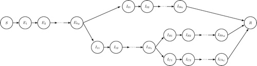
Figure 3. SEIR-type model with heterogeneity in illness severity in which a fraction of infected individuals experience severe illness, and a fraction of those require critical care. This is also a special case of Equations (21(21e) $\begin{array}{rl}\frac{\mathrm{d}R}{\mathrm{d}t}& =(-{\mathbf{A}}_{{\mathbf{I}}_{\mathbf{0}}}\mathbf{1}{)}^{\mathsf{\text{T}}}{\mathbf{y}}_{\mathbf{0}}+(-{\mathbf{A}}_{{\mathbf{I}}_{\mathbf{s}}}\mathbf{1}{)}^{\mathsf{\text{T}}}{\mathbf{y}}_{\mathbf{s}}.\end{array}$(21e) ) (see Figure 2). See the main text for details.

Compare Equations (20(20d) $\begin{array}{rl}\frac{\mathrm{d}R}{\mathrm{d}t}& =r_I{I}_{k_I}+\sum _{j=1}^{k_I-1}(1-{\rho }_{Ij}){\lambda }_{Ij}{I}_j.\end{array}$(20d) ), which assume no births or deaths, to Equations (12) in [64], which assume a simple birth-death process.

2.3. SEIR model with heterogeneity among infected individuals

The examples above illustrate how an existing ODE or DDE model can be generalized or approximated by assuming phase-type distributed dwell times in one or more states. Here we take the generalized SEIR model above and use the GLCT to further explore more complex model assumptions. We do this by considering two special cases of this generalized model (see Figures 2 and 3): one that models hospitalization in a manner that does not change the distribution of time in the infected class, and a second case that models heterogeneity in the severity and duration of disease. In each case, we assume that infected individuals will either experience mild or severe disease with the potential for distributional differences in the duration of infection.

For simplicity, we assume that the removed class R contains both recovered and deceased individuals, and that, upon transitioning from the class of individuals with latent infection (E) to the infectious class (I), a fraction ρ will go on to develop severe symptoms (in state I${}_s$) that may require hospitalization, whereas the remaining fraction ($1-\rho$) do not develop severe disease and thus enter a different state of more mild disease (I${}_0$). Using the GLCT, the states I${}_0$ and I${}_s$ are partitioned into sub-states, where the numbers in each are described by vectors ${\mathbf{y}}_{\mathbf{0}}$ and ${\mathbf{y}}_{\mathbf{s}}$, respectively, and their dynamics obey the following system of ODEs: (21a) $\begin{array}{rl}\frac{\mathrm{d}S}{\mathrm{d}t}& =-\beta SI\end{array}$(21a) (21b) $\begin{array}{rl}\frac{\mathrm{d}\mathbf{x}}{\mathrm{d}t}& ={\mathit{\alpha }}_{\mathbf{E}}\beta SI+{{\mathbf{A}}_{\mathbf{E}}}^{\mathsf{\text{T}}}\mathbf{x}\end{array}$(21b) (21c) $\begin{array}{rl}\frac{\mathrm{d}{\mathbf{y}}_{\mathbf{0}}}{\mathrm{d}t}& ={\mathit{\alpha }}_{{\mathbf{I}}_{\mathbf{0}}}((1-\rho )(-{\mathbf{A}}_{\mathbf{E}}\mathbf{1}{)}^{\mathsf{\text{T}}}\mathbf{x})+{{\mathbf{A}}_{{\mathbf{I}}_{\mathbf{0}}}}^{\mathsf{\text{T}}}{\mathbf{y}}_{\mathbf{0}}\end{array}$(21c) (21d) $\begin{array}{rl}\frac{\mathrm{d}{\mathbf{y}}_{\mathbf{s}}}{\mathrm{d}t}& ={\mathit{\alpha }}_{{\mathbf{I}}_{\mathbf{s}}}(\rho (-{\mathbf{A}}_{\mathbf{E}}\mathbf{1}{)}^{\mathsf{\text{T}}}\mathbf{x})+{{\mathbf{A}}_{{\mathbf{I}}_{\mathbf{s}}}}^{\mathsf{\text{T}}}{\mathbf{y}}_{\mathbf{s}}\end{array}$(21d) (21e) $\begin{array}{rl}\frac{\mathrm{d}R}{\mathrm{d}t}& =(-{\mathbf{A}}_{{\mathbf{I}}_{\mathbf{0}}}\mathbf{1}{)}^{\mathsf{\text{T}}}{\mathbf{y}}_{\mathbf{0}}+(-{\mathbf{A}}_{{\mathbf{I}}_{\mathbf{s}}}\mathbf{1}{)}^{\mathsf{\text{T}}}{\mathbf{y}}_{\mathbf{s}}.\end{array}$(21e)

Equation (21(21e) $\begin{array}{rl}\frac{\mathrm{d}R}{\mathrm{d}t}& =(-{\mathbf{A}}_{{\mathbf{I}}_{\mathbf{0}}}\mathbf{1}{)}^{\mathsf{\text{T}}}{\mathbf{y}}_{\mathbf{0}}+(-{\mathbf{A}}_{{\mathbf{I}}_{\mathbf{s}}}\mathbf{1}{)}^{\mathsf{\text{T}}}{\mathbf{y}}_{\mathbf{s}}.\end{array}$(21e) ) can be viewed as a special case of Equation (15(15d) $\begin{array}{rl}\frac{\mathrm{d}R}{\mathrm{d}t}& =\overbrace{(-{\mathbf{A}}_{\mathbf{I}}\mathbf{1}{)}^{\mathsf{\text{T}}}\mathbf{y}}\end{array}$(15d) ) defined in terms of a mixture of two phase-type distributions, where $\mathbf{y}=[{{\mathbf{y}}_{\mathbf{0}}}^{\mathrm{T}},{{\mathbf{y}}_{\mathbf{s}}}^{\mathrm{T}}]$, the vector ${\mathit{\alpha }}_{\mathit{I}}=[(1-\rho ){\mathit{\alpha }}_{{\mathit{I}}_{\mathbf{0}}}^{\mathrm{T}},\rho {\mathit{\alpha }}_{{\mathit{I}}_{\mathit{s}}}^{\mathrm{T}}]$, and ${\mathbf{A}}_{\mathbf{I}}$ is the block diagonal matrix ${\mathbf{A}}_{\mathbf{I}}=$diag(${\mathbf{A}}_{{\mathbf{I}}_{\mathbf{0}}},{\mathbf{A}}_{{\mathbf{I}}_{\mathbf{s}}}$). The two cases below are described in the context of Equations (21(21e) $\begin{array}{rl}\frac{\mathrm{d}R}{\mathrm{d}t}& =(-{\mathbf{A}}_{{\mathbf{I}}_{\mathbf{0}}}\mathbf{1}{)}^{\mathsf{\text{T}}}{\mathbf{y}}_{\mathbf{0}}+(-{\mathbf{A}}_{{\mathbf{I}}_{\mathbf{s}}}\mathbf{1}{)}^{\mathsf{\text{T}}}{\mathbf{y}}_{\mathbf{s}}.\end{array}$(21e) ).

2.3.1. Case 1: hospitalization independent of progress towards infection resolution

In this scenario, individuals progress towards recovery or death according to an Erlang distribution with rate λ and shape $k_{y_0}$. Independently, they also move towards hospitalization according to an Erlang distributed hospitalization time with rate r and shape $k_H$ (for an example of this structure used to model Ebola, but where $k_H=1$, see [35]). Modeling this with Erlang latent and infectious period distributions (for simplicity) and according to the competing Poisson processes motif detailed in [51] yields a sub-state structure as shown in Figure 2. The matrix-vector pairs ${\mathit{\alpha }}_{\mathbf{E}}$, ${\mathbf{A}}_{\mathbf{E}}$, and ${\mathit{\alpha }}_{{\mathbf{I}}_{\mathbf{0}}}$, ${\mathbf{A}}_{{\mathbf{I}}_{\mathbf{0}}}$ are as described above for Erlang distributions.

The matrix-vector pair ${\mathbf{A}}_{{\mathbf{I}}_{\mathbf{s}}}$ and ${\mathit{\alpha }}_{{\mathbf{I}}_{\mathbf{s}}}$ are defined as follows³. If we order these states starting at the $I_{11}$ entry and work across each rows left to right before moving down to the next row (see Figure 2), then the associated rate matrix has the following block form, with each column and row having $k_H$ blocks of dimension $k_1\times k_1$. This block structure corresponds to each row of the I${}_1$ sub-states shown in the lower portion of Figure 2 as a $k_H\times k_1$ grid of sub-states. This yields (22) ${\mathbf{A}}_{{\mathbf{I}}_{\mathbf{s}}}=\left[\begin{array}{cccccc}{\mathbf{A}}_{\mathbf{d}\mathbf{1}}& {\mathbf{A}}_{\mathbf{s}\mathbf{u}\mathbf{p}}& \mathbf{0}& \mathbf{0}& \cdots & \mathbf{0}\\ \mathbf{0}& {\mathbf{A}}_{\mathbf{d}\mathbf{1}}& {\mathbf{A}}_{\mathbf{s}\mathbf{u}\mathbf{p}}& \mathbf{0}& \cdots & \mathbf{0}\\ \mathbf{0}& \mathbf{0}& {\mathbf{A}}_{\mathbf{d}\mathbf{1}}& {\mathbf{A}}_{\mathbf{s}\mathbf{u}\mathbf{p}}& \ddots & \mathbf{0}\\ ⋮& \ddots & \ddots & \ddots & \ddots & ⋮\\ \mathbf{0}& \mathbf{0}& \mathbf{0}& \mathbf{0}& {\mathbf{A}}_{\mathbf{d}\mathbf{1}}& {\mathbf{A}}_{\mathbf{s}\mathbf{u}\mathbf{p}}\\ \mathbf{0}& \mathbf{0}& \cdots & \mathbf{0}& \mathbf{0}& {\mathbf{A}}_{\mathbf{d}\mathbf{2}}\end{array}\right]$(22) where the diagonal and superdiagonal blocks are (23) ${\mathbf{A}}_{\mathbf{d}\mathbf{1}}=\left[\begin{array}{ccccc}-\lambda -r& \lambda & 0& \cdots & 0\\ 0& \ddots & \lambda & \cdots & 0\\ ⋮& & \ddots & \ddots & ⋮\\ 0& 0& \cdots & \ddots & \lambda \\ 0& 0& \cdots & 0& -\lambda -r\end{array}\right],{\mathbf{A}}_{\mathbf{s}\mathbf{u}\mathbf{p}}=\left[\begin{array}{ccccc}r& 0& 0& \cdots & 0\\ 0& \ddots & 0& \cdots & 0\\ ⋮& & \ddots & \ddots & ⋮\\ 0& 0& \cdots & \ddots & 0\\ 0& 0& \cdots & 0& r\end{array}\right]$(23) and the bottom right diagonal entry is (24) ${\mathbf{A}}_{\mathbf{d}\mathbf{2}}=\left[\begin{array}{ccccc}-\lambda & \lambda & 0& \cdots & 0\\ 0& \ddots & \lambda & \cdots & 0\\ ⋮& & \ddots & \ddots & ⋮\\ 0& 0& \cdots & \ddots & \lambda \\ 0& 0& \cdots & 0& -\lambda \end{array}\right].$(24) Together, the matrix ${\mathbf{A}}_{{\mathbf{I}}_{\mathbf{s}}}$ and the $(k_H{k}_{I_s})\times 1$ initial distribution vector ${\mathit{\alpha }}_{{\mathit{I}}_{\mathit{s}}}=[1,0,\dots ,0{]}^{\mathrm{T}}$ complete the parameterization of model Equations (21(21e) $\begin{array}{rl}\frac{\mathrm{d}R}{\mathrm{d}t}& =(-{\mathbf{A}}_{{\mathbf{I}}_{\mathbf{0}}}\mathbf{1}{)}^{\mathsf{\text{T}}}{\mathbf{y}}_{\mathbf{0}}+(-{\mathbf{A}}_{{\mathbf{I}}_{\mathbf{s}}}\mathbf{1}{)}^{\mathsf{\text{T}}}{\mathbf{y}}_{\mathbf{s}}.\end{array}$(21e) ) to yield the model structure illustrated in Figure 2.

Observe that matrix ${\mathbf{A}}_{{\mathbf{I}}_{\mathbf{s}}}$ above has the same diagonal and superdiagonal blocks in all rows except for the bottom right block, for which the diagonal entries are $-\lambda$ not $-\lambda -r$. Here the dwell time in each sub-state of I${}_s$ (except for the bottom row of sub-states in Figure 2) follows the minimum of two independent exponential distributions with rates λ and r, thus by the properties of exponential distributions, those dwell times are each exponentially distributed with rate $\lambda +r$. Individuals leaving those sub-states then either move horizontally towards resolving their infections, with probability $\lambda /(\lambda +r)$, or move downwards towards hospitalization (the the bottom row of sub-states in Figure 2) with probability $r/(\lambda +r)$ [51]. In the bottom row of sub-states in Figure 2, individuals are hospitalized and can only move horizontally towards the resolution of their illness. This structure ensures that time transition to the hospital (the last row) does not impact their overall distribution of time spent in state I${}_1$.

2.3.2. Case 2: hospitalization with heterogeneous need for critical care

To further illustrate the flexibility of Equations (15(15d) $\begin{array}{rl}\frac{\mathrm{d}R}{\mathrm{d}t}& =\overbrace{(-{\mathbf{A}}_{\mathbf{I}}\mathbf{1}{)}^{\mathsf{\text{T}}}\mathbf{y}}\end{array}$(15d) ) and (21(21e) $\begin{array}{rl}\frac{\mathrm{d}R}{\mathrm{d}t}& =(-{\mathbf{A}}_{{\mathbf{I}}_{\mathbf{0}}}\mathbf{1}{)}^{\mathsf{\text{T}}}{\mathbf{y}}_{\mathbf{0}}+(-{\mathbf{A}}_{{\mathbf{I}}_{\mathbf{s}}}\mathbf{1}{)}^{\mathsf{\text{T}}}{\mathbf{y}}_{\mathbf{s}}.\end{array}$(21e) ), we now consider the model structure illustrated in Figure 3. In this case, we make similar assumptions to the case above, except for the states that pertain to the fraction ρ of individuals who experience severe illness. Those individuals exhibit an Erlang distributed period of relatively mild illness, with rate $r_1$ and shape parameter $k_1$. A fraction f of those individuals recover after an Erlang distributed period of time with rate $r_R$ and shape $k_R$. The remaining fraction $(1-f)$ become even more ill and require hospital care for an Erlang distributed duration of time, with rate $r_C$ and shape $k_C$. As above, all individuals then enter a removed state R which, for our purposes here, makes no distinction between recovery and death.

Comparing Figures 2 and 3, we see that this second scenario is also a special case of Equations (21(21e) $\begin{array}{rl}\frac{\mathrm{d}R}{\mathrm{d}t}& =(-{\mathbf{A}}_{{\mathbf{I}}_{\mathbf{0}}}\mathbf{1}{)}^{\mathsf{\text{T}}}{\mathbf{y}}_{\mathbf{0}}+(-{\mathbf{A}}_{{\mathbf{I}}_{\mathbf{s}}}\mathbf{1}{)}^{\mathsf{\text{T}}}{\mathbf{y}}_{\mathbf{s}}.\end{array}$(21e) ), and only differs from that case in the definition of matrix ${\mathbf{A}}_{{\mathbf{I}}_{\mathbf{s}}}$ and the length $k_1+k_R+k_C$ initial distribution vector ${\mathit{\alpha }}_{{\mathit{I}}_{\mathit{s}}}=[1,0,\dots ,0{]}^{\mathrm{T}}$. Ordering the substates of I${}_s$ from I${}_{11}$ to I${}_{1k_1}$ to I${}_{R1}$ to I${}_{R{k}_R}$ to I${}_{C1}$ to I${}_{C{k}_C}$, then, by the assumptions above, ${\mathbf{A}}_{{\mathbf{I}}_{\mathbf{s}}}$ is given by $\left[\begin{array}{ccc}\begin{array}{ccccc}-r_1& r_1& 0& \cdots & 0\\ 0& -r_1& r_1& \cdots & 0\\ ⋮& & \ddots & \ddots & ⋮\\ 0& 0& \cdots & r_1& r_1\\ 0& 0& \cdots & 0& -r_1\end{array}& \begin{array}{ccccc}0& 0& 0& \cdots & 0\\ 0& \ddots & 0& \cdots & 0\\ ⋮& & \ddots & \ddots & ⋮\\ 0& 0& \cdots & \ddots & 0\\ f{r}_1& 0& \cdots & 0& 0\end{array}& \begin{array}{ccccc}0& 0& 0& \cdots & 0\\ 0& \ddots & 0& \cdots & 0\\ ⋮& & \ddots & \ddots & ⋮\\ 0& 0& \cdots & \ddots & 0\\ (1-f)r_1& 0& \cdots & 0& 0\end{array}\\ \mathbf{0}& \begin{array}{ccccc}-r_R& r_R& 0& \cdots & 0\\ 0& -r_R& r_R& \cdots & 0\\ ⋮& & \ddots & \ddots & ⋮\\ 0& 0& \cdots & -r_R& r_R\\ 0& 0& \cdots & 0& -r_R\end{array}& \mathbf{0}\\ \mathbf{0}& \mathbf{0}& \begin{array}{ccccc}-r_C& r_C& 0& \cdots & 0\\ 0& -r_C& r_C& \cdots & 0\\ ⋮& & \ddots & \ddots & ⋮\\ 0& 0& \cdots & -r_C& r_C\\ 0& 0& \cdots & 0& -r_C\end{array}\end{array}\right].$The two examples above illustrate the utility of deriving models from first principles using the GLCT and basic concepts from Markov chains. This approach can also be leveraged for the analytical study of such models (e.g. see [52]), but as we show in the next section, it can also facilitate the process of computing numerical solutions to such systems of ODEs.

2.4. Benchmarking numerical solutions: LCT vs GLCT

Software like Matlab, Python, Julia, and R, have built-in ODE solvers that implement various numerical methods for obtaining numerical solutions to ODEs. In Figure 4, we summarize the time it takes, using the deSolve package in R [90,101], to compute a numerical solution to the generalized Rosenzweig-MacArthur model with Erlang distributed maturation time and time predators spend in the adult stage, either in the (LCT) form of Equations (10(10d) $\begin{array}{rl}\frac{\mathrm{d}P}{\mathrm{d}t}& =\frac{k}{\tau }{x}_k-\mu P\end{array}$(10d) ) or in the (GLCT) form of Equation (11(11c) $\begin{array}{rl}\frac{\mathrm{d}\mathbf{y}}{\mathrm{d}t}& =\underset{\mathrm{scalar}}{\underbrace{-{\mathbf{1}}^{\mathrm{T}}{{\mathbf{A}}_{\mathbf{X}}}^{\mathrm{T}}\mathbf{x}}}{\mathit{\alpha }}_{\mathbf{P}}+{{\mathbf{A}}_{\mathbf{P}}}^{\mathrm{T}}\mathbf{y}\end{array}$(11c) ). In Figure 5 we make a similar comparison with the SEIR model with Erlang (panel a) and Coxian (panel b) latent and infectious periods, comparing the time it takes to compute numerical solutions to that model in the form of Equation (18(18d) $\begin{array}{rl}\frac{\mathrm{d}R}{\mathrm{d}t}& =\frac{k_I}{{\tau }_I}{I}_{k_I}\end{array}$(18d) ) or the equivalent model in the (GLCT-based) form of Equation (15(15d) $\begin{array}{rl}\frac{\mathrm{d}R}{\mathrm{d}t}& =\overbrace{(-{\mathbf{A}}_{\mathbf{I}}\mathbf{1}{)}^{\mathsf{\text{T}}}\mathbf{y}}\end{array}$(15d) ). See the figure captions further computational details (or the R code that was used to create these figures, available in the Supplementary Materials).

Figure 4. Benchmark results for 140 iterations computing numerical solutions to Rosenzweig-MacArthur model with Erlang (gamma) distributed maturation times and time spent in the adult-stage, using either a direct (LCT; medium grey) or more general (GLCT; black) formulations of the model (the standard Rosenzweig-MacArthur model with no maturation delay and exponentially distributed time spent in the adult stage [light grey; Equations (8(8b) $\begin{array}{rl}\frac{\mathrm{d}P}{\mathrm{d}t}& =\chi \frac{aN}{h+N}P-\mu P\end{array}$(8b) )] is also included as a baseline). The second and third cases are mathematically equivalent systems. For smaller shape parameters (lower dimension systems) the GLCT model formulation is relatively slower than explicitly writing out the 2M + 1 equations, whereas for larger shape parameters (higher dimension systems) the GLCT-based formulation becomes markedly faster. This is likely due to the efficiency of the matrix computations. The x-axis values M indicate the number of maturing predator sub-states ($k_x=M$) and adult predator sub-states ($k_y=M$), which yields a 2M + 1 dimensional model. Numerical solutions were computed using the ode() function in the deSolve package [101] in R [90], using method ode45 with atol=10-6, for time points 0 to 500 in increments of 1, and model parameters r = 1, K = 1000, a = 5, h = 500, $\chi =0.5$, ${\mu }_x=0.5$, ${\mu }_y=1$, with initial conditions $N(0)=1000$, $x_i(0)=0$ ($i\ge 1$), $y_1(0)=10$, and $y_j(0)=0$ (j>1).

Figure 5. Benchmark results for 500 iterations computing numerical solutions to an SEIR model with latent and infectious period distributions that are either Erlang (panel a; Equation (18(18d) $\begin{array}{rl}\frac{\mathrm{d}R}{\mathrm{d}t}& =\frac{k_I}{{\tau }_I}{I}_{k_I}\end{array}$(18d) )) or Coxian (panel b; Equation (20(20d) $\begin{array}{rl}\frac{\mathrm{d}R}{\mathrm{d}t}& =r_I{I}_{k_I}+\sum _{j=1}^{k_I-1}(1-{\rho }_{Ij}){\lambda }_{Ij}{I}_j.\end{array}$(20d) )), using either a direct equation-by-equation formulation (LCT; medium grey) or more general matrix-vector formulation (GLCT; black) of the model (SEIR with exponentially distributed latent and infectious periods [light grey; Equation (14)] also included as a baseline). The second and third cases are mathematically equivalent systems. For smaller shape parameters (lower dimension systems) the GLCT model formulation is relatively slower than explicitly writing out the 2N + 2 equations, whereas for larger shape parameters (higher dimension systems) the GLCT-based formulation becomes faster, presumably due to the efficiency of the matrix computations. The x-axis values N indicate the number of sub-states in each of E ($k_E=N$) and I ($k_I=N$), which yields a 2N + 2 dimensional model. Numerical solutions were computed using the ode() function in the deSolve package [101] in R [90], using method ode45 with atol=10-6, for time points 0 to 100 in increments of 0.5, and model parameters $\beta =1$, ${\mu }_E=4$, ${\mu }_I=7$, where all ${\rho }_E={\rho }_I=0.99$, with initial conditions $S(0)=0.9999$, $E_1(0)=0.0001$, $E_i(0)=0$ (i>1), $I_1(0)=0$, $I_i(0)=0$ (i>1), and $R(0)=0$. See Supplementary Materials for more details.

To summarize these results, neither approach performs uniformly better than the other. In both comparisons, low dimensional models (i.e. smaller shape parameters and thus larger coefficients of variation), coded using the more common equation-by-equation (LCT) model formulation like Equations (10(10d) $\begin{array}{rl}\frac{\mathrm{d}P}{\mathrm{d}t}& =\frac{k}{\tau }{x}_k-\mu P\end{array}$(10d) ), (18(18d) $\begin{array}{rl}\frac{\mathrm{d}R}{\mathrm{d}t}& =\frac{k_I}{{\tau }_I}{I}_{k_I}\end{array}$(18d) ), and (20(20d) $\begin{array}{rl}\frac{\mathrm{d}R}{\mathrm{d}t}& =r_I{I}_{k_I}+\sum _{j=1}^{k_I-1}(1-{\rho }_{Ij}){\lambda }_{Ij}{I}_j.\end{array}$(20d) ), yielded numerical solutions at the same speed as, or faster than, mathematically equivalent models coded using the more general phase-type (GLCT) formulation like Equations (11(11c) $\begin{array}{rl}\frac{\mathrm{d}\mathbf{y}}{\mathrm{d}t}& =\underset{\mathrm{scalar}}{\underbrace{-{\mathbf{1}}^{\mathrm{T}}{{\mathbf{A}}_{\mathbf{X}}}^{\mathrm{T}}\mathbf{x}}}{\mathit{\alpha }}_{\mathbf{P}}+{{\mathbf{A}}_{\mathbf{P}}}^{\mathrm{T}}\mathbf{y}\end{array}$(11c) ) and (15(15d) $\begin{array}{rl}\frac{\mathrm{d}R}{\mathrm{d}t}& =\overbrace{(-{\mathbf{A}}_{\mathbf{I}}\mathbf{1}{)}^{\mathsf{\text{T}}}\mathbf{y}}\end{array}$(15d) ) (see Supplementary Materials for details).

However, for higher dimensional models, the phase-type (GLCT) formulation of these models outperformed their LCT-type counterparts. For a given model family, it is worth noting that these computing speed gains for higher dimensional models are substantially larger than the speed costs associated with low dimensional models. In some cases (see Figure 4), the computing speeds for higher dimensional GLCT-based models were more than twice as fast. These gains are very likely the result of the matrix calculations used in the phase-type (GLCT) formulation of the models being more computationally efficient, and together suggest that the (GLCT-based) matrix-vector model formulations might be preferable in some applications.

Additionally, it is worth noting that the GLCT-based statement of the ODE function only needs to be coded once, as it is agnostic of the number of sub-state variables. For details, see the R code used to create these figures in the Supplementary Materials. In contrast, researchers typically hard-code the number of sub-states for such computations, and thus must write multiple ODE functions to consider models using different shape parameters for the assumed Erlang (or other phase-type) distributions. Thus, taking the time spent writing computer code into consideration, the (GLCT-based) matrix-vector model formulations might again be preferred in many applications.

In summary, these results suggest that the GLCT-based model formulations may allow for significant computing speed improvements, and may simplify the process of writing computer code for use with ODE solvers in R (and similar languages) since a single instance of the model can be used to simulate ODE models of arbitrary number of dimensions.

3. Discussion

ODE models are widely used in the biological sciences, and can often be viewed as mean field models for some (often unspecified) stochastic state transition model [2–4,8,16,35,50]. Such ODE models are sometimes rightfully criticized for their implicit assumption of exponentially distributed dwell times (e.g.exponentially distributed lifetimes of organisms) and their frequent lack of age or stage structure to capture important time lags in the system being modelled, such as the maturation times of organisms or latent periods in disease transmission models [35,36,67,79,80,84,96,110].

In this article, we have provided an overview of the generalized linear chain trick (GLCT) [51], a relatively new tool modellers can use to improve upon existing ODE models to address these shortcomings. We also give an overview of related concepts from Markov chain theory, and have illustrated the utility of the GLCT with some novel applications.

The GLCT [51] extends the well known linear chain trick (LCT) [22,23,33,51,69,70,73, 100,107,108]) to a broad family of probability distributions that includes the phase-type distributions, which are the absorption time distributions for continuous time Markov chains (CTMCs) [15,40,44,66,91]. As such, the GLCT helps to clarify how mean field ODEs reflect underlying stochastic model assumptions when viewed from the perspective of CTMCs [50,52]. The phase-type family of probability distributions includes a number of named probability distributions including exponential, hyperexponential, Erlang (gamma with an integer shape parameter), hypoexponential (generalized Erlang), and Coxian distributions. Importantly, freely available statistical tools exist for fitting phase-type distributions to data, or to other distributions [46,47,77,88]. This enables modellers to build approximate empirical (or other) dwell time distributions into ODE models using the GLCT.

In the Results section above, we derived multiple novel models using the GLCT to illustrate its utility, and we demonstrated some of the computational benefits of using GLCT-based model formulations. Specifically, the GLCT was used to derive extensions of two familiar models: the Rosenzweig-MacArthur predator-prey model, and the SEIR model of infectious disease transmission. We showed how special cases of that generalized SEIR model can be constructed to accommodate additional heterogeneity among infected individuals: the first case models a hospitalization scenario in which the transition to the hospitalized state has no impact on the distribution of the overall time individuals spend sick [cf. [35]], and the second case models heterogeneity in the progression of more severe cases. These examples illustrate how the GLCT can be used to refine model assumptions in a rigorous manner, but without the need to explicitly derive mean field ODEs from stochastic model equations or mean field integral equations.

We also showed some computational benefits of using a GLCT-based approach to ODE model formulation by comparing the time it takes to compute numerical solutions of ODEs using the standard equation-by-equation model formulation or using a GLCT-based approach that entails writing models in a matrix-vector form.

Practically, the first benefit of the GLCT-based approach is that computer code for only one ODE model function definition needs to be written, since it is agnostic of the model dimension (see Supplementary Materials). In contrast, models that have been derived using the standard LCT typically have the number of sub-states hard-coded (since model dimension depends on the shape parameter for the Erlang distributions), and therefore multiple model functions must be coded to explore different shape parameter values. This may be quite beneficial in some applications.

Second, our results show that for low dimensional models the GLCT-based computations are as fast as, or a little slower than, their more traditionally coded counterparts, however for higher dimensional models the GLCT-based model formulations performed best (see Figures 4 and 5). In Figure 4, the GLCT-based approach was more than twice as fast as the traditional approach. We have only demonstrated these benefits for specific examples implemented using the R programming language [90], however, we expect that using other software such as python or Matlab would yield similar results since this improvement in computing time is presumably the result of the computational efficiency of doing matrix and vector based computations. Exploring these computational comparisons in greater detail, with other models and using other computing platforms, would be a useful follow-up to these results. Future work on leveraging the theory of Markov chains and phase-type distributions during analytical investigations of GLCT-based ODE models, as in [52], may also prove to be useful.

This GLCT-based approach to the derivation and application of mean field models does have limitations. While phase-type distributions are dense in the space of univariate probability distributions on $[0,\mathrm{\infty })$, it may not be possible to accurately approximate a given distribution with a phase-type distribution unless a very large number of sub-states are used. For example, distributions with finite support (such as a uniform distribution), or that are heavy-tailed, may not be adequately approximated by a phase-type distribution with only a small number sub-states (or ‘phases’), depending on the application [5,66,105,106].

In conclusion, we hope this work helps other researchers to better understand underlying model assumptions when deriving and evaluating mean field ODE models. We also hope this work demonstrates the relative ease with which some basic intuition from Markov chain theory can be used to specify clear model assumptions from first principles, which can then be very quickly realized as one or more mean field ODE models using the GLCT [49,51].

Acknowledgments

The authors thank Dr. Deena Schmidt, Jillian Kiefer, and the rest of the Mathematical Biology Lab Group at UNR for conversations and comments that improved this manuscript. We also thank two anonymous reviewers for their feedback, and the editors of this issue for their generous accommodation to provide additional time to submit this work during the ongoing SARS-CoV-2/COVID-19 pandemic.

Disclosure statement

No potential conflict of interest was reported by the author(s).

Additional information

Funding

This work was supported by a grant awarded to PJH by the Sloan Scholars Mentoring Network of the Social Science Research Council with funds provided by the Alfred P. Sloan Foundation; and this material is based upon work supported by the National Science Foundation under Grant No. DEB-1929522. This work was partly motivated by PJH's participation in the ICMA-VII conference held at Arizona State University, October 12–14, 2019, with travel support provided to PJH from NSF grant #DMS-1917512 awarded to the Organizing Committee of the ICMA-VII conference.

Notes

1 Gamma distributions with integer-valued shape parameters are those that can be thought of as the sum of independent and identically distributed exponential random variables, and are known as Erlang distributions.

2 The sum of independent exponentially distributed random variables with different rates is known as a generalized Erlang or hypoexponential distribution.

3 Compare to the matrix-vector parameterization of the minimum of two Erlang distributions (the minimum of two phase-type distributions is itself phase-type) using the formulas given in [15].

References

- O.O. Aalen, Phase type distributions in survival analysis, Scand. J. Stat. 22 (1995), pp. 447–463. Available at http://www.jstor.org/stable/4616373.
- L.J.S. Allen, An Introduction to Stochastic Processes with Applications to Biology, 2nd ed., Chapman and Hall/CRC, 2010.
- L.J. Allen, A primer on stochastic epidemic models: formulation, numerical simulation, and analysis, Infect. Dis. Model. 2 (2017), pp. 128–142.
- L. Allen, An Introduction to Mathematical Biology, Pearson/Prentice Hall, Upper Saddle River, NJ, 2007.
- T. Altiok, On the phase-type approximations of general distributions, IIE Trans. 17 (1985), pp. 110–116.
- D. Anderson and R. Watson, On the spread of a disease with gamma distributed latent and infectious periods, Biometrika 67 (1980), pp. 191–198.
- R.M. Anderson, R.M. May, Infectious Diseases of Humans: Dynamics and Control, Oxford University Press, New York, 1992.
- B. Armbruster and E. Beck, Elementary proof of convergence to the mean-field model for the SIR process, J. Math. Biol. 75 (2017), pp. 327–339.
- D.K. Arrowsmith, C.M. Place, An Introduction to Dynamical Systems, Cambridge University Press, New York, 1990.
- M.C. Ausin, M.P. Wiper, and R.E. Lillo, Bayesian estimation of finite time ruin probabilities, Appl. Stoch. Models Bus. Ind. 25 (2009), pp. 787–805.
- N.T.J. Bailey, The Elements of Stochastic Processes with Applications to the Natural Sciences, John Wiley & Sons, New York, 1990.
- A.L. Bertozzi, E. Franco, G. Mohler, M.B. Short, and D. Sledge, The Challenges of Modeling and Forecasting the Spread of COVID-19, Proceedings of the National Academy of Sciences Vol. 117, 2020, pp. 16732–16738
- A. Beuter, L. Glass, M.C. Mackey, and M.S. Titcombe, eds., Nonlinear Dynamics in Physiology and Medicine, Interdisciplinary Applied Mathematics (Book 25), Springer, 2003.
- M. Bladt, B.F. Nielsen, Matrix-Exponential Distributions in Applied Probability, Springer, New York, 2017.
- M. Bladt and B.F. Nielsen, Phase-Type Distributions, in Matrix-Exponential Distributions in Applied Probability, USA, Springer, 2017, pp. 125–197
- D. Champredon, J. Dushoff, and D.J.D. Earn, Equivalence of the Erlang-distributed SEIR epidemic model and the renewal equation, SIAM J. Appl. Math. 78 (2018), pp. 3258–3278.
- G. Chowell, J.M. Hyman, L.M.A. Bettencourt, and C. Castillo-Chavez, eds., Mathematical and Statistical Estimation Approaches in Epidemiology, Springer, Netherlands, 2009.
- G. Clapp and D. Levy, A review of mathematical models for leukemia and lymphoma, Drug Dis. Today: Dis. Models 16 (2015), pp. 1–6.
- D.R. Cox, The analysis of non-markovian stochastic processes by the inclusion of supplementary variables, Math. Proc. Cambridge Philos. Soc. 51 (1955), pp. 433–441.
- D.R. Cox, A use of complex probabilities in the theory of stochastic processes, Math. Proc. Cambridge Philos. Soc. 51 (1955), pp. 313–319.
- A. Cumani, On the canonical representation of homogeneous markov processes modelling failure -- time distributions, Microelectron. Reliab. 22 (1982), pp. 583–602.
- J.M. Cushing, An Introduction to Structured Population Dynamics, Society for Industrial and Applied Mathematics, Philadelphia, PA, 1998.
- J.M. Cushing, Integrodifferential Equations and Delay Models in Population Dynamics, Springer, Berlin Heidelberg, 1977.
- J. Dawes and M. Souza, A derivation of holling's type i, II and III functional responses in predator–prey systems, J. Theor. Biol. 327 (2013), pp. 11–22.
- P. Dayan and L.F. Abbott, Theoretical Neuroscience: Computational and Mathematical Modeling of Neural Systems, Computational Neuroscience, The MIT Press, 2005.
- L. de Pillis, K.R. Fister, W. Gu, C. Collins, M. Daub, D. Gross, J. Moore, and B. Preskill, Mathematical model creation for cancer chemo-immunotherapy, Comput. Math. Methods Med. 10 (2009), pp. 165–184.
- M. Dehon and G. Latouche, A geometric interpretation of the relations between the exponential and generalized Erlang distributions, Adv. Appl. Probabil. 14 (1982), pp. 885–897.
- O. Diekmann and J. Heesterbeek, Mathematical Epidemiology of Infectious Diseases: Model Building, Analysis and Interpretation, Wiley Series in Mathematical and Computational Biology, John Wiley & Sons, LTD, New York, 2000.
- J. Drake, A. Handel, E. O'Dea, and A. Tredennick, A Stochastic Model for the Transmission of SARS-CoV-2 in Georgia, USA, 2020. Available at https://www.covid19.uga.edu/stochastic-fitting-georgia-suplement.html. Accessed: 2020-01-20
- L. Edelstein-Keshet, Mathematical Models in Biology, Classics in Applied Mathematics (Book 46), Society for Industrial and Applied Mathematics, 2005.
- S.P. Ellner, J. Guckenheimer, Dynamic Models in Biology, Princeton University Press, Princeton, NJ, 2006.
- M. Fackrell, Modelling healthcare systems with phase-type distributions, Health Care Manage. Sci.12 (2008), pp. 11–26.
- D. Fargue, Réductibilité des systèmes héréditaires à des systèmes dynamiques (régis par des équations différentielles ou aux dérivées partielles), C. R. Acad. Sci. Paris Sér. A-B 277 (1973), pp. B471–B473MR 0333630
- Z. Feng, D. Xu, and H. Zhao, Epidemiological models with non-exponentially distributed disease stages and applications to disease control, Bull. Math. Biol. 69 (2007), pp. 1511–1536.
- Z. Feng, Y. Zheng, N. Hernandez-Ceron, H. Zhao, J.W. Glasser, and A.N. Hill, Mathematical models of Ebola-Consequences of underlying assumptions, Math. Biosci. 277 (2016), pp. 89–107.
- W.M. Getz, C.R. Marshall, C.J. Carlson, L. Giuggioli, S.J. Ryan, S.S. Romañach, C. Boettiger, S.D. Chamberlain, L. Larsen, P. D'Odorico, and D. O'Sullivan, Making ecological models adequate, Ecol. Lett. 21 (2018), pp. 153–166.
- Q.M. He and H. Zhang, PH-invariant polytopes and coxian representations of phase type distributions, Stoch. Models 22 (2006), pp. 383–409.
- Q.M. He and H. Zhang, Coxian approximations of matrix-exponential distributions, Calcolo 44 (2007), pp. 235–264.
- M.W. Hirsch, S. Smale, and R.L. Devaney, Differential Equations, Dynamical Systems, and an Introduction to Chaos, 3rd ed., Elsevier, 2013.
- A. Hobolth, A. Siri-Jégousse, and M. Bladt, Phase-type distributions in population genetics, Theor. Popul. Biol. 127 (2019), pp. 16–32.
- C.S. Holling, The components of predation as revealed by a study of small-mammal predation of the european pine sawfly, Can. Entomol. 91 (1959), pp. 293–320.
- C.S. Holling, Some characteristics of simple types of predation and parasitism, Can. Entomol. 91 (1959), pp. 385–398.
- S. Hoops, R. Hontecillas, V. Abedi, A. Leber, C. Philipson, A. Carbo, J. Bassaganya-Riera, Ordinary Differential Equations (ODEs) Based Modeling, in Computational Immunology, Josep Bassaganya-Riera, eds., Elsevier, San Diego, CA, 2016. pp. 63–78.
- A. Horváth, M. Scarpa, and M. Telek, Phase Type and Matrix Exponential Distributions in Stochastic Modeling, in Principles of Performance and Reliability Modeling and Evaluation: Essays in Honor of Kishor Trivedi on his 70th Birthday, L. Fiondella and A. Puliafito, eds., Springer International Publishing, Cham, 2016, pp. 3–25
- G. Horváth, P. Reinecke, M. Telek, and K. Wolter, Efficient Generation of PH-Distributed Random Variates, in Proceedings of the 19th international conference on Analytical and Stochastic Modeling Techniques and Applications, K. Al-Begain, D. Fiems, and J.M. Vincent, eds., Berlin, Heidelberg, Springer, 2012, pp. 271–285.
- G. Horváth and M. Telek, BuTools 2: A Rich Toolbox for Markovian Performance Evaluation, in ValueTools 2016 -- 10th EAI International Conference on Performance Evaluation Methodologies and Tools, 1. Association for Computing Machinery, 2017, pp. 137–142
- G. Horváth and M. Telek, Butools v2.0. Available at http://webspn.hit.bme.hu/%7Etelek/tools/butools/doc/index.html (2020). Accessed: 2020-05-15
- S.K. Howard and M. Taylor, An Introduction to Stochastic Modeling, 3rd ed., Academic Press, 1998.
- P. Hurtado and C. Richards, A procedure for deriving new ODE models: using the generalized linear chain trick to incorporate phase-type distributed delay and dwell time assumptions, Math. Appl. Sci. Eng. 9999 (2020), pp. 1–14.
- P.J. Hurtado, Building New Models: Rethinking and Revising ODE Model Assumptions, in Foundations for Undergraduate Research in Mathematics, Hannah Callender Highlander, Alex Capaldi, Carrie Diaz Eaton, ed., Springer International Publishing, Birkhäuser, Cham, 2020. pp. 1–86.
- P.J. Hurtado and A.S. Kirosingh, Generalizations of the ‘linear chain trick’: incorporating more flexible dwell time distributions into mean field ODE models, J. Math. Bio. 79 (2019), pp. 1831–1883.
- P.J. Hurtado and C. Richards, Finding reproduction numbers for epidemic models & predator-prey models of arbitrary finite dimension using the generalized linear chain trick (2020). arXiv:2008.06768
- E.M. Izhikevich, Dynamical Systems in Neuroscience: The Geometry of Excitability and Bursting, Computational Neuroscience, MIT Press, 2010.
- M.J. Keeling and B.T. Grenfell, Disease extinction and community size: modeling the persistence of measles, Science 275 (1997), pp. 65–67.
- M.J. Keeling and B.T. Grenfell, Understanding the persistence of measles: reconciling theory, simulation and observation, Proc. R. Soc. Lond. Ser. B: Biol. Sci. 269 (2002), pp. 335–343.
- J. Keener and J. Sneyd, Mathematical Physiology I: Cellular Physiology, 2nd ed., Springer, 2008.
- J. Keener and J. Sneyd, Mathematical Physiology II: Systems Physiology, 2nd ed., Springer, 2008.
- W.O. Kermack and A.G. McKendrick, A contribution to the mathematical theory of epidemics, Proc. R. Soc. Lond. Ser. A, Containing Papers Math. Phys. Charact. 115 (1927), pp. 700–721.
- W.O. Kermack and A.G. McKendrick, Contributions to the mathematical theory of epidemics. II. The problem of endemicity, Proc. R. Soc. Lond. Ser. A, Containing Papers Math. Phys. Character 138 (1932), pp. 55–83.
- W.O. Kermack and A.G. McKendrick, Contributions to the mathematical theory of epidemics. III. Further studies of the problem of endemicity, Proc. R. Soc. Lond. Ser. A, Containing Papers Math. Phys. Character 141 (1933), pp. 94–122Available at http://www.jstor.org/stable/96207
- W.O. Kermack and A.G. McKendrick, Contributions to the mathematical theory of epidemics – i, Bull. Math. Biol. 53 (1991), pp. 33–55.
- W.O. Kermack and A.G. McKendrick, Contributions to the mathematical theory of epidemics – II. the problem of endemicity, Bull. Math. Biol. 53 (1991), pp. 57–87.
- W.O. Kermack and A.G. McKendrick, Contributions to the mathematical theory of epidemics – III. further studies of the problem of endemicity, Bull. Math. Biol. 53 (1991), pp. 89–118.
- S. Kim, J.H. Byun, and I.H. Jung, Global stability of an SEIR epidemic model where empirical distribution of incubation period is approximated by Coxian distribution, Adv. Diff. Equ. 2019 (2019).
- D. Kirschner and J.C. Panetta, Modeling immunotherapy of the tumor -- immune interaction, J. Math. Biol. 37 (1998), pp. 235–252.
- Z. Komárková, Phase-type approximation techniques, Bachelor's Thesis, Masaryk University, 2012. Available at https://is.muni.cz/th/ysfsq/
- O. Krylova and D.J.D. Earn, Effects of the infectious period distribution on predicted transitions in childhood disease dynamics, J. R. Soc. Interface 10 (2013).
- A.L. Lloyd, The dependence of viral parameter estimates on the assumed viral life cycle: limitations of studies of viral load data, Proc. R. Soc. Lond. B: Biol. Sci. 268 (2001), pp. 847–854.
- A.L. Lloyd, Destabilization of epidemic models with the inclusion of realistic distributions of infectious periods, Proc. R. Soc. Lond. B: Biol. Sci. 268 (2001), pp. 985–993.
- A.L. Lloyd, Realistic distributions of infectious periods in epidemic models: changing patterns of persistence and dynamics, Theor. Popul. Biol. 60 (2001), pp. 59–71.
- A.L. Lloyd, Sensitivity of Model-Based Epidemiological Parameter Estimation to Model Assumptions, in Mathematical and Statistical Estimation Approaches in Epidemiology, G. Chowell, J.M. Hyman, L.M.A. Bettencourt, and C. Castillo-Chavez, eds., Springer, Netherlands, Dordrecht, 2009, pp. 123–141
- J. Ma and D.J.D. Earn, Generality of the final size formula for an epidemic of a newly invading infectious disease, Bull. Math. Biol. 68 (2006), pp. 679–702.
- N. MacDonald, Time Lags in Biological Models, Lecture Notes in Biomathematics, Vol. 27, Springer, Verlag Berlin Heidelberg, 1978.
- A.H. Marshall and S.I. McClean, Using coxian phase-Type distributions to identify patient characteristics for duration of stay in hospital, Health Care Manage. Sci. 7 (2004), pp. 285–289.
- A.H. Marshall and M. Zenga, Experimenting with the coxian phase-Type distribution to uncover suitable fits, Methodol. Comput. Appl. Probab. 14 (2010), pp. 71–86.
- K.S. McCann, Food Webs, Monographs in Population Biology (Book 57), Princeton University Press, 2011.
- C. McGrory, A. Pettitt, and M. Faddy, A fully Bayesian approach to inference for Coxian phase-type distributions with covariate dependent mean, Comput. Stat. Data Anal. 53 (2009), pp. 4311–4321.
- J.D. Meiss, Differential Dynamical Systems, Revised ed., Society for Industrial and Applied Mathematics, Philadelphia, PA, 2017.
- J.A.J. Metz and O. Diekmann, eds., The Dynamics of Physiologically Structured Populations, Lecture Notes in Biomathematics, Vol. 68, Springer, Berlin, Heidelberg, 1986.
- J. Metz and O. Diekmann, Exact finite dimensional representations of models for physiologically structured populations. I: The abstract formulation of linear chain trickery, in Proceedings of Differential Equations With Applications in Biology, Physics, and Engineering 1989, J.A. Goldstein, F. Kappel, and W. Schappacher, eds., Vol. 133, 1991, pp. 269–289
- W.W. Murdoch, C.J. Briggs, and R.M. Nisbet, Consumer–Resource Dynamics, Monographs in Population Biology , Vol. 36, Princeton University Press, Princeton, USA, 2003.
- J.D. Murray, Mathematical Biology: I. An Introduction, Interdisciplinary Applied Mathematics (Book 17), Springer, 2007.
- A. Nande, B. Adlam, J. Sheen, M.Z. Levy, and A.L. Hill, Dynamics of COVID-19 under social distancing measures are driven by transmission network structure, PLOS Comput. Biol. 17 (2021), p. e1008684.
- R.M. Nisbet, W.S.C. Gurney, and J.A.J. Metz, Stage Structure Models Applied in Evolutionary Ecology, in Applied Mathematical Ecology, S.A. Levin, T.G. Hallam, and L.J. Gross, eds., Springer, Berlin, Heidelberg, 1989, pp. 428–449
- C.A. O'Cinneide, On non-uniqueness of representations of phase-type distributions, Commun. Stat. Stoch. Models 5 (1989), pp. 247–259.
- C.A. O'Cinneide, Characterization of phase-type distributions, Commun. Stat. Stoch. Models 6 (1990), pp. 1–57.
- C.A. O'Cinneide, Phase-type distributions: open problems and a few properties, Commun. Stat. Stoch. Models 15 (1999), pp. 731–757.
- H. Okamura and T. Dohi, Mapfit: An R-Based Tool for PH/MAP Parameter Estimation, in Proceedings of the 12th International Conference on Quantitative Evaluation of Systems, J. Campos and B.R. Haverkort, eds., QEST 2015 Vol. 9259, New York, NY, USA. Springer-Verlag, New York, Inc., 2015, pp. 105–112
- T. Osogami and M. Harchol-Balter, Closed form solutions for mapping general distributions to quasi-minimal PH distributions, Perform. Eval. 63 (2006), pp. 524–552.
- R Core Team, A Language and Environment for Statistical Computing, R Foundation for Statistical Computing, Vienna, Austria , 2020. Available at https://www.R-project.org/.
- P. Reinecke, L. Bodrog, and A. Danilkina, Phase-Type Distributions, in Resilience Assessment and Evaluation of Computing Systems, K. Wolter, A. Avritzer, M. Vieira, and A. van Moorsel, eds., Springer, Berlin, Heidelberg, 2012, pp. 85–113
- P. Reinecke, T. Krauß, and K. Wolter, Cluster-based fitting of phase-type distributions to empirical data, Comput. Math. Appl. 64 (2012), pp. 3840–3851.
- M. Renardy, M. Eisenberg, and D. Kirschner, Predicting the second wave of COVID-19 in washtenaw county, MI, J. Theor. Biol. 507 (2020), p. 110461.
- S.I. Resnick, Adventures in Stochastic Processes, Birkhäuser, Boston, 2002.
- J. Rizk, K. Burke, and C. Walsh, On the Non-uniqueness of Representations of Coxian Phase-Type Distributions (2019). arXiv:1901.03849v2
- S.L. Robertson, S.M. Henson, T. Robertson, and J.M. Cushing, A matter of maturity: to delay or not to delay? continuous-time compartmental models of structured populations in the literature 2000-2016, Nat. Resour. Model. 31 (2018), pp. e12160.
- M.L. Rosenzweig and R.H. MacArthur, Graphical representation and stability conditions of predator-prey interactions, Am. Nat. 97 (1963), pp. 209–223.
- R. Sachs, L. Hlatky, and P. Hahnfeldt, Simple ode models of tumor growth and anti-angiogenic or radiation treatment, Math. Comput. Model. 33 (2001), pp. 1297–1305.
- H.M.T. Samuel Karlin, A First Course in Stochastic Processes, 2nd ed., Academic Press, 1975.
- H. Smith, An Introduction to Delay Differential Equations with Applications to the Life Sciences, Vol. 57, Springer Science & Business Media, 2010.
- K. Soetaert, T. Petzoldt, and R.W. Setzer, Solving differential equations in R: package deSolve, J. Stat. Softw. 33 (2010), pp. 1–25Available at http://www.jstatsoft.org/v33/i09
- W.J. Stewart, Introduction to the Numerical Solution of Markov Chains, Princeton University Press, Princeton, NJ, 1994.
- S.H. Strogatz, Nonlinear Dynamics and Chaos: With Applications to Physics, Biology, Chemistry, and Engineering, Studies in Nonlinearity, 2nd ed., Westview Press, 2014.
- X. Tang, Z. Luo, and J.C. Gardiner, Modeling hospital length of stay by Coxian phase-type regression with heterogeneity, Stat. Med. 31 (2012), pp. 1502–1516.
- E. Vatamidou, I. Adan, M. Vlasiou, and B. Zwart, On the accuracy of phase-type approximations of heavy-tailed risk models, Scand. Actuar. J. 2014 (2012), pp. 510–534.
- S. Venturini, F. Dominici, and G. Parmigiani, Gamma shape mixtures for heavy-tailed distributions, Ann. Appl. Stat. 2 (2008), pp. 756–776.
- T. Vogel, Systèmes déferlants, systèmes héréditaires, systèmes dynamiques, in Proceedings of the International Symposium Nonlinear Vibrations, IUTAM, Kiev, 1961, pp. 123–130
- T. Vogel, Théorie des Systèmes Évolutifs, no. 22 in Traité de physique théorique et de physique mathématique, Gauthier-Villars, Paris, 1965
- X. Wang, Y. Shi, Z. Feng, and J. Cui, Evaluations of interventions using mathematical models with exponential and non-exponential distributions for disease stages: the case of ebola, Bull. Math. Biol. 79 (2017), pp. 2149–2173.
- H.J. Wearing, P. Rohani, and M.J. Keeling, Appropriate models for the management of infectious diseases, PLOS Med. 2 (2005).
- S. Wiggins, Introduction to Applied Nonlinear Dynamical Systems and Chaos, 2nd ed., Texts in Applied Mathematics, Vol. 2, Springer-Verlag, New York, 2003.
- J. Xia, Z. Liu, R. Yuan, and S. Ruan, The effects of harvesting and time delay on predator-prey systems with holling type II functional response, SIAM J. Appl. Math. 70 (2009), pp. 1178–1200.
- C.A. Yates, M.J. Ford, and R.L. Mort, A multi-stage representation of cell proliferation as a Markov process, Bull. Math. Biol. 79 (2017), pp. 2905–2928.