The impact of poaching and regime switching on the dynamics of single-species model

ABSTRACT

It is widely recognized that the criminal act of poaching has brought tremendous damage to biodiversity. This paper employs a stochastic single-species model with regime switching to investigate the impact of poaching. We first carry out the survival analysis and obtain sufficient conditions for the extinction and persistence in mean of the single-species population. Then, we show that the model is positive recurrent by constructing suitable Lyapunov function. Finally, numerical simulations are carried out to support our theoretical results. It is found that: (i) As the intensity of poaching increases, the odds of being at risk of extinction increases for the single-species population. (ii) The regime switching can suppress the extinction of the single-species population. (iii) The white noise is detrimental to the survival of the single-species population. (iv) Increasing the criminal cost of poaching and establishing animal sanctuaries are important ways to protect biodiversity.

Keywords:

• Stochastic single species model
• poaching
• regime switching
• positive recurrent
• survival analysis

2010 Mathematics Subject Classifications:

• 60H10
• 92D25

1. Introduction

Poaching has led to the reduction and disappearance of many species around the world and has a major impact on the structure and function of ecosystems. For example, the tibetan antelopes are hunted for their extremely soft, light and warm underfur which is usually obtained after death to make luxury items at high prices. However, because rarity makes the living species attractive, their overexploitation can remain profitable, rendering such species even rarer, or driving them to extinction. This phenomenon is called the anthropogenic Allee effect where species rarity increases price, and therefore, the incentive to harvest, driving small populations extinct [9, 13]. In addition, Kenney et al. [19] demonstrated that a critical zone exists in which a small, incremental increase in poaching greatly increases the probability of extinction, by using an individual-based, stochastic spatial model based on extensive field data. Hence, to prevent the biological resources from destruction and protect the ecological environment, various measures have been proposed. For instance, many countries have clearly regarded poaching as a crime (for example, in China, poaching may face more than 10 years in prison); at the beginning of the twentieth century, forest and ungulate species were protected and either recovered naturally or by means of planting or reintroduction. Nowadays, large carnivores are strictly protected or managed by quotas in many countries of the world, and great efforts are undertaken to protect and conserve their recovering populations [26]. These efforts led to successful conservation measures for some species, e.g. wolf [6] and Eurasian Lynx [7]. However, other species still face strong population declines, because the illegal harvest (i.e. poaching) of wild resources is an open access system and is driven by economic interests, it is difficult for the law to exert sufficient protection [4, 5, 8], e.g. lion[3] and tiger [27].

Among the effective measures, the approach of providing protected areas has become most popular over the past decades. The impact of protected areas in renewing biological resources and protecting the population was quantitatively investigated by Kar and Matsuda [17]. They found that protected patches are an effective means of conserving resource populations. Dubey et al. [10] investigated the dynamics of a fishery resource model with migrations between two patches and showed that even if fishery is exploited continuously in the unreserved zone, fish populations can be maintained at an appropriate equilibrium level in the habitat. In addition, as shown in May [24], Gard [11, 12], the growth rates in population systems should be stochastic owing to random noises, and as a result, the solution of the system will not tend to a steady positive point but fluctuate around some average values. Hu et al. [14–16] pointed out that fluctuating environmental conditions, temperature and rainfall, in particular, influence the growth of populations strongly: Temperature affects the mortality, while rainfall supplies water in breeding sites in the wild area for the survival. Therefore, it is important to investigate the effect of random noises in the environment on population dynamics. For example, Zou and Wang [35] studied the dynamics of stochastic model for a single species with protection zone and showed that the establishment of nature reserves can protect endangered species effectively in good conditions. In particular, Wei and Wang [31] considered the following stochastic model for a single species with migrations between two different patches: (1) $\left\{\begin{array}{l}\mathrm{d}{x}_t=\left[x_t(a-b{x}_t)-m_1{x}_t+m_2{y}_t-E_1{x}_t\right]\mathrm{d}t+\sigma x_t\mathrm{d}{B}_t,\\ \mathrm{d}{y}_t=\left[y_t(a-b{y}_t)-m_2{y}_t+m_1{x}_t-E_2{y}_t\right]\mathrm{d}t+\sigma y_t\mathrm{d}{B}_t,\end{array}\right.$(1) where $x_t$, $y_t$ are the densities of population in the unprotected environment and the protected one at time t, respectively. a is the intrinsic growth rate, $\frac{a}{b}$ is the carrying capacity of the environment, $m_1$ is the migration rate to the nature reserve from the unprotected area, $m_2$ is the migration rate to the unprotected area from the nature reserve, $E_1$, $E_2$ are the intensity of poaching in the unprotected area and the nature reserve, respectively, and assume that illegal hunting takes place within two patches for pursuing high prices with restriction $E_2<E_1$. $B_t$ is a standard Brownian motion. ${\sigma }^2$ is the intensity of white noise. In [31], it is proved that for any initial value $(x_0,y_0)\in {\mathbb{R}}_{+}^2$, there exists a unique global solution to (1(1) $\left\{\begin{array}{l}\mathrm{d}{x}_t=\left[x_t(a-b{x}_t)-m_1{x}_t+m_2{y}_t-E_1{x}_t\right]\mathrm{d}t+\sigma x_t\mathrm{d}{B}_t,\\ \mathrm{d}{y}_t=\left[y_t(a-b{y}_t)-m_2{y}_t+m_1{x}_t-E_2{y}_t\right]\mathrm{d}t+\sigma y_t\mathrm{d}{B}_t,\end{array}\right.$(1) ) that remains in ${\mathbb{R}}_{+}^2$ almost surely, and then they provided sufficient conditions for the persistence in mean and extinction of the species.

As shown in [29], the usual state in nature is that the population fluctuates around a trend or a stable average. However, many studies have shown that smooth change can be interrupted by a sudden shift to a completely different regime. For example, after a long period in which vegetation cover fluctuated around a gradually declining trend of vegetation cover, the Sahara region collapsed suddenly into a desert in ancient times [28]; an abrupt climate change, whether warming or cooling, wetting or drying, could have lasting and profound impacts on natural ecosystems [1]. Just as Assaf et al. [2] pointed out that the white noise cannot describe the phenomena that the population may suffer sudden catastrophic shocks or alien species invasion in nature. Therefore, it is necessary to introduce telegraph noise, which can be illustrated as a switching between two or more regimes of environment [30]. Frequently, the switching among different environments is memoryless and the waiting time for the next switch is exponentially distributed [20–22, 33, 34, 36]. Thus we can model the regime switching by a continuous-time Markov chain with values in a finite state space, which drives the changes of the parameters of population models with state switchings of the Markov chain. Inspired by the above facts, in the present paper, we model the random by a continuous-time Markov chain $\left\{r\right(t),t\ge 0\}$ in a finite state space $\mathbb{S}=\{1,2,\cdot \cdot \cdot ,N\}$ with generator $\mathrm{\Gamma }=({\gamma }_{ij}{)}_{N\times N}$ given by $\mathbb{P}\left\{r\right(t+\mathrm{\Delta })=j|r(t)=i\}=\left\{\begin{array}{ll}{\gamma }_{ij}\mathrm{\Delta }+o\left(\mathrm{\Delta }\right)& \mathrm{i}\mathrm{f}i\ne j,\\ 1+{\gamma }_{ij}\mathrm{\Delta }+o\left(\mathrm{\Delta }\right)& \mathrm{i}\mathrm{f}i=j,\end{array}\right.$ where ${\gamma }_{ij}\ge 0$ for $i,j=1,2,\cdot \cdot \cdot ,N$ with $i\ne j$ and ${\gamma }_{ii}=-\sum _{i\ne j}{\gamma }_{ij}$ for each $i=1,2,\cdot \cdot \cdot ,N.$ Assume Markov chain $r\left(t\right)$ is irreducible and independent of Brownian motion. Therefore, there exists a unique stationary distribution $\pi =\{{\pi }_1,{\pi }_2,\cdot \cdot \cdot ,{\pi }_N\}$ of $r\left(t\right)$ which satisfies $\pi \mathrm{\Gamma }=0,\sum _{i=1}^N{\pi }_i=1$ and ${\pi }_i>0,\mathrm{\forall }i\in \mathbb{S}$. Then we can further obtain the following model with regime switching: (2) $\left\{\begin{array}{l}\mathrm{d}{x}_t=\left[x_t(a_{r\left(t\right)}-b_{r\left(t\right)}{x}_t)-m_{1_{r\left(t\right)}}{x}_t+m_{2_{r\left(t\right)}}{y}_t-E_{1_{r\left(t\right)}}{x}_t\right]\mathrm{d}t+{\sigma }_{r\left(t\right)}{x}_t\mathrm{d}{B}_t,\\ \mathrm{d}{y}_t=\left[y_t(a_{r\left(t\right)}-b_{r\left(t\right)}{y}_t)-m_{2_{r\left(t\right)}}{y}_t+m_{1_{r\left(t\right)}}{x}_t-E_{2_{r\left(t\right)}}{y}_t\right]\mathrm{d}t+{\sigma }_{r\left(t\right)}{y}_t\mathrm{d}{B}_t,\end{array}\right.$(2) where $a_i$, $b_i$, $m_{1_i}$, $m_{2_i}$, $E_{1_i}$, $E_{2_i}$, and ${\sigma }_i$ are all positive constants, and $E_{2_i}<E_{1_i}$ for any $i\in \mathbb{S}$.

This article formulates a stochastic single species model with regime switching and the impact of poaching. Our main idea is to investigate the effect of poaching and the telegraph noise on the dynamics of single species. The rest of this article is organized as follows: We first present some preliminaries and basic results of the model in Section 2. Then in Section 3, we present the main results of system (1.2). In Section 4, we present the detailed proof of the theoretical results. In Section 5, some numerical simulations are carried out to illustrate the obtained results. Finally, in Section 6, we give a brief discussion and the summary of the main results.

2. Preliminaries

Throughout this paper, unless otherwise specified, we let $(\mathrm{\Omega },\mathcal{F},\{{\mathcal{F}}_t{\}}_{t\ge 0},\mathbb{P})$ be a complete probability space with a filtration $\{{\mathcal{F}}_t{\}}_{t\ge 0}$ satisfying the usual conditions (i.e. it is right continuous and ${\mathcal{F}}_0$ contains all P-null sets).

For the convenience of discussion, we let ${\mathbb{R}}_{+}^n=\{x\in {\mathbb{R}}^n:x_i>0,i=1,2,\cdot \cdot \cdot ,n\}$, $|x|=\sqrt{\sum _{i=1}^n{x}_i^2}$, $\hat{f}=\underset{i\in \mathbb{S}}{min}f\left(i\right)$, $\check{f}=\underset{i\in \mathbb{S}}{max}f\left(i\right)$.

Next, we give some results on the stationary distribution for stochastic differential equations under regime switching. For more details, we can refer the readers to [32]. Consider the following equation: (3) $\mathrm{d}{x}_t=b(x_t,r(t\left)\right)\mathrm{d}t+\sigma (x_t,r(t\left)\right)\mathrm{d}{B}_t,$(3) where $B_t$ is the d-dimensional Brownian motion, and $b(\cdot ,\cdot ):{\mathbb{R}}^n\times \mathbb{S}\to {\mathbb{R}}^n$, $\sigma (\cdot ,\cdot ):{\mathbb{R}}^n\times \mathbb{S}\to {\mathbb{R}}^{n\times d}$ satisfying $\sigma (x,k){\sigma }^T(x,k)=\left(d_{ij}\right(x,k\left)\right)$. Let $x_t\in {\mathbb{R}}^n$ be a solution of the model (3(3) $\mathrm{d}{x}_t=b(x_t,r(t\left)\right)\mathrm{d}t+\sigma (x_t,r(t\left)\right)\mathrm{d}{B}_t,$(3) ) for any given initial value $(x_0,r(0\left)\right)$. Let $V(x_t,k)$ be any twice continuously differentiable function for any given $k\in \mathbb{S}$, the operator L of system (3(3) $\mathrm{d}{x}_t=b(x_t,r(t\left)\right)\mathrm{d}t+\sigma (x_t,r(t\left)\right)\mathrm{d}{B}_t,$(3) ) can be defined by $LV(x,k)=\sum _{i=1}^N{b}_i(x,k)\frac{\mathrm{\partial }V(x,k)}{\mathrm{\partial }{x}_i}+\frac{1}{2}\sum _{i,j=1}^N{d}_{ij}(x,k)\frac{{\mathrm{\partial }}^{2}V(x,k)}{\mathrm{\partial }{x}_i\mathrm{\partial }{x}_j}+\sum _{i=1}^N{\gamma }_{kj}V(x,k).$ In view of the generalized It$\hat{o}$'s formula [25], one can get that $\mathrm{d}V(x_t,r(t\left)\right)=LV(x_t,r(t\left)\right)\mathrm{d}t+\sigma (x_t,r(t\left)\right)\frac{\mathrm{\partial }V(x_t,r(t\left)\right)}{\mathrm{\partial }{x}_t}\mathrm{d}{B}_t.$ In the sequel, we shall introduce the definition of the positive recurrent and give some fundamental results.

Definition 2.1

[32]

If $\mathbb{P}\{{\tau }^x<\mathrm{\infty }\}=1$ for any $x\notin E$, where $x=\varphi \left(0\right)$ and ${\tau }^x$ is the hitting time of E for ${\varphi }^x\left(t\right)$ i.e. the first time that the process ${\varphi }^x\left(t\right)$ enters the set E, or ${\tau }^x:=\{t\ge 0:{\varphi }^x(t)\in E\}$, then process ${\varphi }^x\left(t\right)$ is said to be positive recurrent with respect to some nonempty bounded open subset E of ${\mathbb{R}}^n$, that is, $\mathbb{E}\left[{\tau }^x\right]<\mathrm{\infty }$ for any $x\notin E$.

Lemma 2.1

[32]

Model (3(3) $\mathrm{d}{x}_t=b(x_t,r(t\left)\right)\mathrm{d}t+\sigma (x_t,r(t\left)\right)\mathrm{d}{B}_t,$(3) ) is positive recurrent if the following condition is satisfied: there exists a bounded open subset D of ${\mathbb{R}}^n$ with a regular (i.e. smooth) boundary satisfying that, for each $k\in \mathbb{S}$ there exists a nonnegative function $V(\cdot ,k):D^c\to \mathbb{R}$ such that $V(\cdot ,k)$ is twice continuously differentiable and that for some $\alpha >0$, $LV(x,k)\le -\alpha ,\text{for any }(x,k)\in D^c\times \mathbb{S}.$

Remark 2.1

According to Theorem 4.3 in [32], one can see that the positive recurrent process $(x_t,r(t\left)\right)$ has a unique stationary distribution.

Lemma 2.2

[18]

Consider the following linear system of equations (4) $\mathrm{\Gamma }c=\eta ,$(4) where $c,\eta \in {\mathbb{R}}^N$. Suppose that $\mathrm{\Gamma }=({\gamma }_{ij}{)}_{N\times N}$ is irreducible. Then Equation (4(4) $\mathrm{\Gamma }c=\eta ,$(4) ) has a solution if and only if $\pi \eta =0$.

3. Main results

To investigate the dynamical behaviour of stochastic model (2(2) $\left\{\begin{array}{l}\mathrm{d}{x}_t=\left[x_t(a_{r\left(t\right)}-b_{r\left(t\right)}{x}_t)-m_{1_{r\left(t\right)}}{x}_t+m_{2_{r\left(t\right)}}{y}_t-E_{1_{r\left(t\right)}}{x}_t\right]\mathrm{d}t+{\sigma }_{r\left(t\right)}{x}_t\mathrm{d}{B}_t,\\ \mathrm{d}{y}_t=\left[y_t(a_{r\left(t\right)}-b_{r\left(t\right)}{y}_t)-m_{2_{r\left(t\right)}}{y}_t+m_{1_{r\left(t\right)}}{x}_t-E_{2_{r\left(t\right)}}{y}_t\right]\mathrm{d}t+{\sigma }_{r\left(t\right)}{y}_t\mathrm{d}{B}_t,\end{array}\right.$(2) ), the first concerning thing is whether the solution is global and positive.

Theorem 3.1

For any initial value $(x_0,y_0,r(0\left)\right)\in {\mathbb{R}}_{+}^2\times \mathbb{S}$, there is a unique solution $(x_t,y_t)$ of model (2(2) $\left\{\begin{array}{l}\mathrm{d}{x}_t=\left[x_t(a_{r\left(t\right)}-b_{r\left(t\right)}{x}_t)-m_{1_{r\left(t\right)}}{x}_t+m_{2_{r\left(t\right)}}{y}_t-E_{1_{r\left(t\right)}}{x}_t\right]\mathrm{d}t+{\sigma }_{r\left(t\right)}{x}_t\mathrm{d}{B}_t,\\ \mathrm{d}{y}_t=\left[y_t(a_{r\left(t\right)}-b_{r\left(t\right)}{y}_t)-m_{2_{r\left(t\right)}}{y}_t+m_{1_{r\left(t\right)}}{x}_t-E_{2_{r\left(t\right)}}{y}_t\right]\mathrm{d}t+{\sigma }_{r\left(t\right)}{y}_t\mathrm{d}{B}_t,\end{array}\right.$(2) ) on $t\ge 0$, and the solution will remain in ${\mathbb{R}}_{+}^2$ with probability 1.

Corollary 3.1

The solution $(x_t,y_t)$ established in Theorem 3.1 satisfies $\underset{t\to \mathrm{\infty }}{lim sup}[x_t+y_t]<\mathrm{\infty }\mathrm{a}.\mathrm{s}.$ Moreover, the solution of system (2(2) $\left\{\begin{array}{l}\mathrm{d}{x}_t=\left[x_t(a_{r\left(t\right)}-b_{r\left(t\right)}{x}_t)-m_{1_{r\left(t\right)}}{x}_t+m_{2_{r\left(t\right)}}{y}_t-E_{1_{r\left(t\right)}}{x}_t\right]\mathrm{d}t+{\sigma }_{r\left(t\right)}{x}_t\mathrm{d}{B}_t,\\ \mathrm{d}{y}_t=\left[y_t(a_{r\left(t\right)}-b_{r\left(t\right)}{y}_t)-m_{2_{r\left(t\right)}}{y}_t+m_{1_{r\left(t\right)}}{x}_t-E_{2_{r\left(t\right)}}{y}_t\right]\mathrm{d}t+{\sigma }_{r\left(t\right)}{y}_t\mathrm{d}{B}_t,\end{array}\right.$(2) ) has the properties that (5) $\underset{t\to \mathrm{\infty }}{lim sup}\frac{\ln x_t}{t}\le 0\mathrm{a}\mathrm{n}\mathrm{d}\underset{t\to \mathrm{\infty }}{lim sup}\frac{\ln y_t}{t}\le 0.$(5)

Next, we will study some asymptotic properties of model (2(2) $\left\{\begin{array}{l}\mathrm{d}{x}_t=\left[x_t(a_{r\left(t\right)}-b_{r\left(t\right)}{x}_t)-m_{1_{r\left(t\right)}}{x}_t+m_{2_{r\left(t\right)}}{y}_t-E_{1_{r\left(t\right)}}{x}_t\right]\mathrm{d}t+{\sigma }_{r\left(t\right)}{x}_t\mathrm{d}{B}_t,\\ \mathrm{d}{y}_t=\left[y_t(a_{r\left(t\right)}-b_{r\left(t\right)}{y}_t)-m_{2_{r\left(t\right)}}{y}_t+m_{1_{r\left(t\right)}}{x}_t-E_{2_{r\left(t\right)}}{y}_t\right]\mathrm{d}t+{\sigma }_{r\left(t\right)}{y}_t\mathrm{d}{B}_t,\end{array}\right.$(2) ), such as the extinction, persistence of the single-species population in the natural environment and the nature reserve. We establish the following theorem.

Theorem 3.2

Let $(x_t,y_t)$ be a solution of model (2(2) $\left\{\begin{array}{l}\mathrm{d}{x}_t=\left[x_t(a_{r\left(t\right)}-b_{r\left(t\right)}{x}_t)-m_{1_{r\left(t\right)}}{x}_t+m_{2_{r\left(t\right)}}{y}_t-E_{1_{r\left(t\right)}}{x}_t\right]\mathrm{d}t+{\sigma }_{r\left(t\right)}{x}_t\mathrm{d}{B}_t,\\ \mathrm{d}{y}_t=\left[y_t(a_{r\left(t\right)}-b_{r\left(t\right)}{y}_t)-m_{2_{r\left(t\right)}}{y}_t+m_{1_{r\left(t\right)}}{x}_t-E_{2_{r\left(t\right)}}{y}_t\right]\mathrm{d}t+{\sigma }_{r\left(t\right)}{y}_t\mathrm{d}{B}_t,\end{array}\right.$(2) ) with any initial value $(x_0,y_0,r(0\left)\right)\in {\mathbb{R}}_{+}^2\times \mathbb{S}$. Then we have the following results:

1. $\underset{t\to \mathrm{\infty }}{lim}{x}_t=0$, $\underset{t\to \mathrm{\infty }}{lim}{y}_t=0$, i.e. species in the nature reserve and the natural environment are always extinct, if $\sum _{i=1}^N{\pi }_i(a_i-\frac{{\sigma }_i^2}{2}-E_{2_i})<0$.

2. $\underset{t\to \mathrm{\infty }}{lim inf}\frac{1}{t}{\int }_0^t{x}_s\mathrm{d}s>0$, $\underset{t\to \mathrm{\infty }}{lim inf}\frac{1}{t}{\int }_0^t{y}_s\mathrm{d}s>0$, i.e. species in the nature reserve and the natural environment are always persistent in mean, if $\sum _{i=1}^N{\pi }_i\left[\right(a_i-\frac{{\sigma }_i^2}{2})-E_{1_i}-m_{1_i}]>0$ and $\sum _{i=1}^N{\pi }_i\left[\right(a_i-\frac{{\sigma }_i^2}{2})-E_{2_i}-m_{2_i}]>0$.

Now, we study the existence of a stationary distribution of the positive solutions to model (2(2) $\left\{\begin{array}{l}\mathrm{d}{x}_t=\left[x_t(a_{r\left(t\right)}-b_{r\left(t\right)}{x}_t)-m_{1_{r\left(t\right)}}{x}_t+m_{2_{r\left(t\right)}}{y}_t-E_{1_{r\left(t\right)}}{x}_t\right]\mathrm{d}t+{\sigma }_{r\left(t\right)}{x}_t\mathrm{d}{B}_t,\\ \mathrm{d}{y}_t=\left[y_t(a_{r\left(t\right)}-b_{r\left(t\right)}{y}_t)-m_{2_{r\left(t\right)}}{y}_t+m_{1_{r\left(t\right)}}{x}_t-E_{2_{r\left(t\right)}}{y}_t\right]\mathrm{d}t+{\sigma }_{r\left(t\right)}{y}_t\mathrm{d}{B}_t,\end{array}\right.$(2) ). The existence of a stationary distribution can be regarded as the stochastic weak stability of the model. For the sake of convenience and simplicity, we introduce the following notations: $\begin{array}{rl}{\lambda }_i& :=[2(a_i+\sqrt{m_{1_i}{m}_{2_i}}-\frac{{\sigma }_i^2}{2})-(E_{1_i}+E_{2_i})-(m_{1_i}+m_{2_i})\\ & -max\{\frac{(a_i+b_i-E_{1_i}{)}^2}{4b_i},\frac{(a_i+b_i-E_{2_i}{)}^2}{4b_i}\}].\end{array}$

Theorem 3.3

If $\sum _{i=1}^N{\pi }_i{\lambda }_i>0$, then for any initial value $(x_0,y_0,r(0\left)\right)\in {\mathbb{R}}_{+}^2\times \mathbb{S}$, the solution $(x_t,y_t)$ of model (2(2) $\left\{\begin{array}{l}\mathrm{d}{x}_t=\left[x_t(a_{r\left(t\right)}-b_{r\left(t\right)}{x}_t)-m_{1_{r\left(t\right)}}{x}_t+m_{2_{r\left(t\right)}}{y}_t-E_{1_{r\left(t\right)}}{x}_t\right]\mathrm{d}t+{\sigma }_{r\left(t\right)}{x}_t\mathrm{d}{B}_t,\\ \mathrm{d}{y}_t=\left[y_t(a_{r\left(t\right)}-b_{r\left(t\right)}{y}_t)-m_{2_{r\left(t\right)}}{y}_t+m_{1_{r\left(t\right)}}{x}_t-E_{2_{r\left(t\right)}}{y}_t\right]\mathrm{d}t+{\sigma }_{r\left(t\right)}{y}_t\mathrm{d}{B}_t,\end{array}\right.$(2) ) is positive recurrent with respect to the domain $D_{ϵ}=\left\{\right(x,y)\in {\mathbb{R}}_{+}^2:ϵ\le x\le \frac{1}{ϵ},ϵ\le y\le \frac{1}{ϵ}\}$, where $0<ϵ<1$ is a sufficiently small constant. Moreover, model (2(2) $\left\{\begin{array}{l}\mathrm{d}{x}_t=\left[x_t(a_{r\left(t\right)}-b_{r\left(t\right)}{x}_t)-m_{1_{r\left(t\right)}}{x}_t+m_{2_{r\left(t\right)}}{y}_t-E_{1_{r\left(t\right)}}{x}_t\right]\mathrm{d}t+{\sigma }_{r\left(t\right)}{x}_t\mathrm{d}{B}_t,\\ \mathrm{d}{y}_t=\left[y_t(a_{r\left(t\right)}-b_{r\left(t\right)}{y}_t)-m_{2_{r\left(t\right)}}{y}_t+m_{1_{r\left(t\right)}}{x}_t-E_{2_{r\left(t\right)}}{y}_t\right]\mathrm{d}t+{\sigma }_{r\left(t\right)}{y}_t\mathrm{d}{B}_t,\end{array}\right.$(2) ) has a unique stationary distribution $\pi (\cdot )$.

It is noteworthy to mention that if $m_{1_{r\left(t\right)}}=m_{2_{r\left(t\right)}}=0$ for $\mathrm{\forall }r\left(t\right)\in \mathbb{S}$, that is, model (2(2) $\left\{\begin{array}{l}\mathrm{d}{x}_t=\left[x_t(a_{r\left(t\right)}-b_{r\left(t\right)}{x}_t)-m_{1_{r\left(t\right)}}{x}_t+m_{2_{r\left(t\right)}}{y}_t-E_{1_{r\left(t\right)}}{x}_t\right]\mathrm{d}t+{\sigma }_{r\left(t\right)}{x}_t\mathrm{d}{B}_t,\\ \mathrm{d}{y}_t=\left[y_t(a_{r\left(t\right)}-b_{r\left(t\right)}{y}_t)-m_{2_{r\left(t\right)}}{y}_t+m_{1_{r\left(t\right)}}{x}_t-E_{2_{r\left(t\right)}}{y}_t\right]\mathrm{d}t+{\sigma }_{r\left(t\right)}{y}_t\mathrm{d}{B}_t,\end{array}\right.$(2) ) without protection zone, which simply becomes the following stochastic model (6) $\mathrm{d}{x}_t=\left[x_t(a_{r\left(t\right)}-b_{r\left(t\right)}{x}_t)-E_{r\left(t\right)}{x}_t\right]\mathrm{d}t+{\sigma }_{r\left(t\right)}{x}_t\mathrm{d}{B}_t.$(6) Similarly, we can obtain the following result.

Corollary 3.2

For model (6(6) $\mathrm{d}{x}_t=\left[x_t(a_{r\left(t\right)}-b_{r\left(t\right)}{x}_t)-E_{r\left(t\right)}{x}_t\right]\mathrm{d}t+{\sigma }_{r\left(t\right)}{x}_t\mathrm{d}{B}_t.$(6) ), the following assertions hold.

(i)	For any initial value $(x_0,y_0,r(0\left)\right)\in {\mathbb{R}}_{+}^2\times \mathbb{S}$, there is a unique solution $x_t$ of model (6(6) $\mathrm{d}{x}_t=\left[x_t(a_{r\left(t\right)}-b_{r\left(t\right)}{x}_t)-E_{r\left(t\right)}{x}_t\right]\mathrm{d}t+{\sigma }_{r\left(t\right)}{x}_t\mathrm{d}{B}_t.$(6) ) on $t\ge 0$, and the solution will remain in ${\mathbb{R}}_{+}^2$ with probability 1.
(ii)	$\underset{t\to \mathrm{\infty }}{lim}{x}_t=0$, i.e. the single species is extinct, if $\sum _{i=1}^N{\pi }_i(a_i-\frac{{\sigma }_i^2}{2}-E_i)<0$.
(iii)	$\underset{t\to \mathrm{\infty }}{lim inf}\frac{1}{t}{\int }_0^t{x}_s\mathrm{d}s>0$, i.e. the single species is persistent in mean, if $\sum _{i=1}^N{\pi }_i(a_i-\frac{{\sigma }_i^2}{2}-E_i)>0$.
(iv)	If $\sum _{i=1}^N{\pi }_i{\xi }_i>0$, then for any initial value $(x_0,y_0,r(0\left)\right)\in {\mathbb{R}}_{+}^2\times \mathbb{S}$, the solution $x_t$ of model (6(6) $\mathrm{d}{x}_t=\left[x_t(a_{r\left(t\right)}-b_{r\left(t\right)}{x}_t)-E_{r\left(t\right)}{x}_t\right]\mathrm{d}t+{\sigma }_{r\left(t\right)}{x}_t\mathrm{d}{B}_t.$(6) ) is positive recurrent with respect to the domain $D_{ϵ}=\{x\in {\mathbb{R}}_{+}:ϵ\le x\le \frac{1}{ϵ}\}$, where $0<ϵ<1$ is a sufficiently small constant. Moreover, model (6(6) $\mathrm{d}{x}_t=\left[x_t(a_{r\left(t\right)}-b_{r\left(t\right)}{x}_t)-E_{r\left(t\right)}{x}_t\right]\mathrm{d}t+{\sigma }_{r\left(t\right)}{x}_t\mathrm{d}{B}_t.$(6) ) has a unique stationary distribution $\pi (\cdot )$. Here ${\xi }_i:=a_i-\frac{{\sigma }_i^2}{2}-E_i.$

Remark 3.1

The proof of Theorem 3.1 is very similar to Theorem 2.1 in Wei and Wang [31] and is omitted. The proof of Corollary 3.1 is provided in Appendix A.

4. Proofs of main results

In this section, we provide the detailed proofs of the main results illustrated in Section 3.

4.1. Proof of theorem 3.2

Proof.

By the generalized It$\hat{o}$'s formula, one can see that (7) $\begin{array}{rl}d\ln (x_1+x_2)& =(a_{r\left(t\right)}-\frac{{\sigma }_{r\left(t\right)}^2}{2}-\frac{E_{1_{r\left(t\right)}}x+E_{2_{r\left(t\right)}}y+b_{r\left(t\right)}(x^2+y^2)}{x+y})\mathrm{d}t+{\sigma }_{r\left(t\right)}\mathrm{d}{B}_t\\ & \le (a_{r\left(t\right)}-\frac{1}{2}{\sigma }_{r\left(t\right)}^2-E_{2_{r\left(t\right)}})\mathrm{d}t+{\sigma }_{r\left(t\right)}\mathrm{d}{B}_t,\end{array}$(7) here we have applied the hypotheses $E_{2_{r\left(t\right)}}<E_{1_{r\left(t\right)}}$ $\mathrm{\forall }r\left(t\right)\in \mathbb{S}$. Integrating both sides from 0 to t and dividing by t, one can see that (8) $\frac{\ln (x_t+y_t)-\ln (x_0+y_0)}{t}\le \frac{{\int }_0^t(a_{r\left(\tau \right)}-\frac{{\sigma }_{r\left(\tau \right)}^2}{2}-E_{2_{r\left(\tau \right)}})d\tau }{t}+\frac{G_t}{t},$(8) where $G_t={\int }_0^t{\sigma }_{r\left(\tau \right)}\mathrm{d}{B}_{\tau }$. Note that $G_t$ is a local martingales, whose quadratic variation is $〈G_t,G_t{〉}_t={\int }_0^t{\sigma }_{r\left(\tau \right)}^{2}d\tau \le {\check{\sigma }}^{2}t$. It follows from the strong law of large numbers for martingales (see [23]) that (9) $\underset{t\to \mathrm{\infty }}{lim}\frac{G_t}{t}=0\mathrm{a}.\mathrm{s}.$(9) Equations (8(8) $\frac{\ln (x_t+y_t)-\ln (x_0+y_0)}{t}\le \frac{{\int }_0^t(a_{r\left(\tau \right)}-\frac{{\sigma }_{r\left(\tau \right)}^2}{2}-E_{2_{r\left(\tau \right)}})d\tau }{t}+\frac{G_t}{t},$(8) ) and (9(9) $\underset{t\to \mathrm{\infty }}{lim}\frac{G_t}{t}=0\mathrm{a}.\mathrm{s}.$(9) ) and the ergodic theorem of Markov chain $r\left(t\right)$ give $\begin{array}{rl}\underset{t\to \mathrm{\infty }}{lim sup}\frac{\ln (x_t+y_t)}{t}& \le \underset{t\to \mathrm{\infty }}{lim}\frac{{\int }_0^t(a_{r\left(\tau \right)}-\frac{{\sigma }_{r\left(\tau \right)}^2}{2}-E_{2_{r\left(\tau \right)}})d\tau }{t}\\ & =\sum _{i=1}^N{\pi }_i(a_i-\frac{{\sigma }_i^2}{2}-E_{2_i})\mathrm{a}.\mathrm{s}.\end{array}$ That is, when $\sum _{i=1}^N\pi (a_i-\frac{{\sigma }_i^2}{2}-E_{2_i})<0$, then $\underset{t\to \mathrm{\infty }}{lim}(x_t+y_t)=0$, which implies that $\underset{t\to \mathrm{\infty }}{lim}{x}_t=0,\underset{t\to \mathrm{\infty }}{lim}{y}_t=0\mathrm{a}.\mathrm{s}.$ This completes the proof of (i).

Now we prove (ii). By using generalized It$\hat{o}$'s formula to system (2(2) $\left\{\begin{array}{l}\mathrm{d}{x}_t=\left[x_t(a_{r\left(t\right)}-b_{r\left(t\right)}{x}_t)-m_{1_{r\left(t\right)}}{x}_t+m_{2_{r\left(t\right)}}{y}_t-E_{1_{r\left(t\right)}}{x}_t\right]\mathrm{d}t+{\sigma }_{r\left(t\right)}{x}_t\mathrm{d}{B}_t,\\ \mathrm{d}{y}_t=\left[y_t(a_{r\left(t\right)}-b_{r\left(t\right)}{y}_t)-m_{2_{r\left(t\right)}}{y}_t+m_{1_{r\left(t\right)}}{x}_t-E_{2_{r\left(t\right)}}{y}_t\right]\mathrm{d}t+{\sigma }_{r\left(t\right)}{y}_t\mathrm{d}{B}_t,\end{array}\right.$(2) ) results in (10) $\begin{array}{rl}d\ln x_t& =\left(a_{r\left(t\right)}-m_{1_{r\left(t\right)}}-E_{1_{r\left(t\right)}}-\frac{{\sigma }_{r\left(t\right)}^2}{2}-b_{r\left(t\right)}x+m_{2_{r\left(t\right)}}\frac{y}{x}\right)\mathrm{d}t+{\sigma }_{r\left(t\right)}\mathrm{d}{B}_t\\ & \ge \left(a_{r\left(t\right)}-m_{1_{r\left(t\right)}}-E_{1_{r\left(t\right)}}-\frac{{\sigma }_{r\left(t\right)}^2}{2}-\check{b}x\right)\mathrm{d}t+{\sigma }_{r\left(t\right)}\mathrm{d}{B}_t.\end{array}$(10) Integrating from 0 to t and dividing by t on both sides of (10(10) $\begin{array}{rl}d\ln x_t& =\left(a_{r\left(t\right)}-m_{1_{r\left(t\right)}}-E_{1_{r\left(t\right)}}-\frac{{\sigma }_{r\left(t\right)}^2}{2}-b_{r\left(t\right)}x+m_{2_{r\left(t\right)}}\frac{y}{x}\right)\mathrm{d}t+{\sigma }_{r\left(t\right)}\mathrm{d}{B}_t\\ & \ge \left(a_{r\left(t\right)}-m_{1_{r\left(t\right)}}-E_{1_{r\left(t\right)}}-\frac{{\sigma }_{r\left(t\right)}^2}{2}-\check{b}x\right)\mathrm{d}t+{\sigma }_{r\left(t\right)}\mathrm{d}{B}_t.\end{array}$(10) ) yields (11) $\frac{1}{t}\ln \frac{x_t}{x_0}\ge \frac{1}{t}{\int }_0^t(a_{r\left(\tau \right)}-m_{1_{r\left(\tau \right)}}-E_{1_{r\left(\tau \right)}}-\frac{{\sigma }_{r\left(\tau \right)}^2}{2}-\check{b}x)d\tau +\frac{G_t}{t}.$(11) Equations (5(5) $\underset{t\to \mathrm{\infty }}{lim sup}\frac{\ln x_t}{t}\le 0\mathrm{a}\mathrm{n}\mathrm{d}\underset{t\to \mathrm{\infty }}{lim sup}\frac{\ln y_t}{t}\le 0.$(5) ), (9(9) $\underset{t\to \mathrm{\infty }}{lim}\frac{G_t}{t}=0\mathrm{a}.\mathrm{s}.$(9) ) and (11(11) $\frac{1}{t}\ln \frac{x_t}{x_0}\ge \frac{1}{t}{\int }_0^t(a_{r\left(\tau \right)}-m_{1_{r\left(\tau \right)}}-E_{1_{r\left(\tau \right)}}-\frac{{\sigma }_{r\left(\tau \right)}^2}{2}-\check{b}x)d\tau +\frac{G_t}{t}.$(11) ) and the ergodic theorem of Markov chain $r\left(t\right)$ give $\underset{t\to \mathrm{\infty }}{lim inf}\frac{1}{t}{\int }_0^t{x}_s\mathrm{d}s\ge \frac{1}{\check{b}}\sum _{i=1}^N{\pi }_i[a_i-E_{1_i}-m_{1_i}-\frac{{\sigma }_i^2}{2}]>0\mathrm{a}.\mathrm{s}.$ Similarly, we can have that $\underset{t\to \mathrm{\infty }}{lim inf}\frac{1}{t}{\int }_0^t{y}_s\mathrm{d}s\ge \frac{1}{\check{b}}\sum _{i=1}^N{\pi }_i[a_i-E_{2_i}-m_{2_i}-\frac{{\sigma }_i^2}{2}]>0\mathrm{a}.\mathrm{s}.$ This completes the proof of (ii).

4.2. Proof of theorem 3.3

Proof.

According to Theorem 3.1, we can derive that for any initial value $(x_0,y_0,r_0)\in {\mathbb{R}}_{+}^2\times \mathbb{S}$, the solution of system (2(2) $\left\{\begin{array}{l}\mathrm{d}{x}_t=\left[x_t(a_{r\left(t\right)}-b_{r\left(t\right)}{x}_t)-m_{1_{r\left(t\right)}}{x}_t+m_{2_{r\left(t\right)}}{y}_t-E_{1_{r\left(t\right)}}{x}_t\right]\mathrm{d}t+{\sigma }_{r\left(t\right)}{x}_t\mathrm{d}{B}_t,\\ \mathrm{d}{y}_t=\left[y_t(a_{r\left(t\right)}-b_{r\left(t\right)}{y}_t)-m_{2_{r\left(t\right)}}{y}_t+m_{1_{r\left(t\right)}}{x}_t-E_{2_{r\left(t\right)}}{y}_t\right]\mathrm{d}t+{\sigma }_{r\left(t\right)}{y}_t\mathrm{d}{B}_t,\end{array}\right.$(2) ) is regular.

Note that $\pi =\{{\pi }_1,{\pi }_2,\cdot \cdot \cdot ,{\pi }_N\}$, and $\sum _{i=1}^N{\pi }_i=1,$ then $\pi [\lambda -\pi \lambda {\mathbb{I}}_N]=0,$ where $\lambda =({\lambda }_1,{\lambda }_2,\cdot \cdot \cdot ,{\lambda }_N{)}^T$, ${\mathbb{I}}_N=(1,1,\cdot \cdot \cdot ,1)\in {\mathbb{R}}^N$. It follows from Lemma 2.2 that the linear equation (12) $\mathrm{\Gamma }\varpi =\lambda -\pi \lambda {\mathbb{I}}_N$(12) has a solution $\varpi =({\varpi }_1,{\varpi }_2,\cdot \cdot \cdot ,{\varpi }_N{)}^T\in {\mathbb{R}}^N$. From (12(12) $\mathrm{\Gamma }\varpi =\lambda -\pi \lambda {\mathbb{I}}_N$(12) ), it is easy to find that (13) $-{\lambda }_i+\sum _{j=1}^N{\gamma }_{ij}{\varpi }_j=-\sum _{i=1}^N{\pi }_i{\lambda }_i.$(13) Then, define a $C^2$-function $V:{\mathbb{R}}_{+}^2\to {\mathbb{R}}_{+}$ by (14) $(x_1-\ln x_1-1)+(x_2-\ln x_2-1)+({\varpi }_i+|\varpi |),$(14) where$|\varpi |=\sqrt{{\varpi }_1^2+{\varpi }_2^2+\cdot \cdot \cdot +{\varpi }_N^2}$. Using generalized It$\hat{o}$'s formula to (13(13) $-{\lambda }_i+\sum _{j=1}^N{\gamma }_{ij}{\varpi }_j=-\sum _{i=1}^N{\pi }_i{\lambda }_i.$(13) ) yields $\begin{array}{rl}LV& =(a_i+b_i-E_{1_i})x-b_i{x}^2+(a_i+b_i-E_{2_i})y-b_i{y}^2\\ & -(2a_i-{\sigma }_i^2-m_{1_i}-m_{2_i}-E_{1_i}-E_{2_i})-\left(\frac{m_{2_i}y}{x}+\frac{m_{1_i}x}{y}\right)+\sum _{j=1}^N{\gamma }_{ij}{\varpi }_j\\ & \le (a_i+b_i-E_{1_i})x-b_i{x}^2+(a_i+b_i-E_{2_i})y-b_i{y}^2\\ & -{\lambda }_i-max\left\{\frac{(a_i+b_i-E_{1_i}{)}^2}{4b_i},\frac{(a_i+b_i-E_{2_i}{)}^2}{4b_i}\right\}+\sum _{j=1}^N{\gamma }_{ij}{\varpi }_j\\ & =(a_i+b_i-E_{1_i})x-b_i{x}^2+(a_i+b_i-E_{2_i})y-b_i{y}^2-\sum _{j=1}^N{\pi }_i{\lambda }_i\\ & -max\left\{\frac{(a_i+b_i-E_{1_i}{)}^2}{4b_i},\frac{(a_i+b_i-E_{2_i}{)}^2}{4b_i}\right\}.\end{array}$ Now define a bounded closed set $D_{ϵ}$ by $D_{ϵ}=\left\{(x,y)\in {\mathbb{R}}_{+}^2:ϵ\le x\le \frac{1}{ϵ},ϵ\le y\le \frac{1}{ϵ}\right\},$ where $0<ϵ<1$ is a sufficiently small constant such that $\begin{array}{rl}& (a_i+b_i-E_{1_i})ϵ-\sum _{j=1}^N{\pi }_i{\lambda }_i<0,(a_i+b_i-E_{2_i})ϵ-\sum _{j=1}^N{\pi }_i{\lambda }_i<0,\\ & (a_i+b_i-E_{1_i}){ϵ}^{-1}-b_i{ϵ}^{-2}<0,(a_i+b_i-E_{2_i}){ϵ}^{-1}-b_i{ϵ}^{-2}<0.\end{array}$ For convenience, we divide ${\mathbb{R}}_{+}^2\setminus D_{ϵ}$ into four domains $\begin{array}{rl}{D}_1& =\left\{\right(x,y)\in {\mathbb{R}}_{+}^2:0<x<ϵ\},D_2=\left\{\right(x,y)\in {\mathbb{R}}_{+}^2:0<y<ϵ\},\\ D_3& =\left\{\right(x,y)\in {\mathbb{R}}_{+}^2:x>\frac{1}{ϵ}\},D_4=\left\{\right(x,y)\in {\mathbb{R}}_{+}^2:y>\frac{1}{ϵ}\}.\end{array}$ Clearly, ${\mathbb{R}}_{+}^2\setminus D_{ϵ}=D_1\cup D_2\cup D_3\cup D_4$. Next, we will prove $LV(x,y)<0$ for any $(x,y)\in {\mathbb{R}}_{+}^2\setminus D_{ϵ}$.

Case 1. If $(x,y)\in D_1$, we have $\begin{array}{rl}LV& \le (a_i+b_i-E_{1_i})x-b_i{x}^2+(a_i+b_i-E_{2_i})y-b_i{y}^2-\sum _{j=1}^N{\pi }_i{\lambda }_i\\ & -max\left\{\frac{(a_i+b_i-E_{1_i}{)}^2}{4b_i},\frac{(a_i+b_i-E_{2_i}{)}^2}{4b_i}\right\}\\ & \le (a_i+b_i-E_{1_i})ϵ-\sum _{j=1}^N{\pi }_i{\lambda }_i<0.\end{array}$ Case 2. In domain $D_2$, $\begin{array}{rl}LV& \le (a_i+b_i-E_{1_i})x-b_i{x}^2+(a_i+b_i-E_{2_i})y-b_i{y}^2-\sum _{j=1}^N{\pi }_i{\lambda }_i\\ & -max\left\{\frac{(a_i+b_i-E_{1_i}{)}^2}{4b_i},\frac{(a_i+b_i-E_{2_i}{)}^2}{4b_i}\right\}\\ & \le (a_i+b_i-E_{2_i})ϵ-\sum _{j=1}^N{\pi }_i{\lambda }_i<0.\end{array}$ Case 3. In domain $D_3$, $\begin{array}{rl}LV& \le (a_i+b_i-E_{1_i})x-b_i{x}^2+(a_i+b_i-E_{2_i})y-b_i{y}^2-\sum _{j=1}^N{\pi }_i{\lambda }_i\\ & -max\left\{\frac{(a_i+b_i-E_{1_i}{)}^2}{4b_i},\frac{(a_i+b_i-E_{2_i}{)}^2}{4b_i}\right\}\\ & \le (a_i+b_i-E_{1_i}){ϵ}^{-1}-b_i{ϵ}^{-2}<0.\end{array}$ Case 4. In domain $D_4$, $\begin{array}{rl}LV& \le (a_i+b_i-E_{1_i})x-b_i{x}^2+(a_i+b_i-E_{2_i})y-b_i{y}^2-\sum _{j=1}^N{\pi }_i{\lambda }_i\\ & -max\left\{\frac{(a_i+b_i-E_{1_i}{)}^2}{4b_i},\frac{(a_i+b_i-E_{2_i}{)}^2}{4b_i}\right\}\\ & \le (a_i+b_i-E_{2_i}){ϵ}^{-1}-b_i{ϵ}^{-2}<0.\end{array}$ Consequently $LV(x,y)<0\mathrm{f}\mathrm{o}\mathrm{r}\mathrm{\forall }(x,y)\in {\mathbb{R}}_{+}^2\setminus D_{ϵ}.$ It then follows from Lemma 2.1 that the solution of model (2(2) $\left\{\begin{array}{l}\mathrm{d}{x}_t=\left[x_t(a_{r\left(t\right)}-b_{r\left(t\right)}{x}_t)-m_{1_{r\left(t\right)}}{x}_t+m_{2_{r\left(t\right)}}{y}_t-E_{1_{r\left(t\right)}}{x}_t\right]\mathrm{d}t+{\sigma }_{r\left(t\right)}{x}_t\mathrm{d}{B}_t,\\ \mathrm{d}{y}_t=\left[y_t(a_{r\left(t\right)}-b_{r\left(t\right)}{y}_t)-m_{2_{r\left(t\right)}}{y}_t+m_{1_{r\left(t\right)}}{x}_t-E_{2_{r\left(t\right)}}{y}_t\right]\mathrm{d}t+{\sigma }_{r\left(t\right)}{y}_t\mathrm{d}{B}_t,\end{array}\right.$(2) ) is positive recurrent with respect to the domain $D_{ϵ}$. Moreover, according to Remark 2.1, we know that model (2(2) $\left\{\begin{array}{l}\mathrm{d}{x}_t=\left[x_t(a_{r\left(t\right)}-b_{r\left(t\right)}{x}_t)-m_{1_{r\left(t\right)}}{x}_t+m_{2_{r\left(t\right)}}{y}_t-E_{1_{r\left(t\right)}}{x}_t\right]\mathrm{d}t+{\sigma }_{r\left(t\right)}{x}_t\mathrm{d}{B}_t,\\ \mathrm{d}{y}_t=\left[y_t(a_{r\left(t\right)}-b_{r\left(t\right)}{y}_t)-m_{2_{r\left(t\right)}}{y}_t+m_{1_{r\left(t\right)}}{x}_t-E_{2_{r\left(t\right)}}{y}_t\right]\mathrm{d}t+{\sigma }_{r\left(t\right)}{y}_t\mathrm{d}{B}_t,\end{array}\right.$(2) ) admits a unique stationary distribution.

5. Numerical simulations

In this section, we will numerically illustrate the effects of the Markov chain, poaching and the migration rates $m_1$, $m_2$ on survival of species by several examples. Here, we only focus on the intrinsic growth rate of model (2(2) $\left\{\begin{array}{l}\mathrm{d}{x}_t=\left[x_t(a_{r\left(t\right)}-b_{r\left(t\right)}{x}_t)-m_{1_{r\left(t\right)}}{x}_t+m_{2_{r\left(t\right)}}{y}_t-E_{1_{r\left(t\right)}}{x}_t\right]\mathrm{d}t+{\sigma }_{r\left(t\right)}{x}_t\mathrm{d}{B}_t,\\ \mathrm{d}{y}_t=\left[y_t(a_{r\left(t\right)}-b_{r\left(t\right)}{y}_t)-m_{2_{r\left(t\right)}}{y}_t+m_{1_{r\left(t\right)}}{x}_t-E_{2_{r\left(t\right)}}{y}_t\right]\mathrm{d}t+{\sigma }_{r\left(t\right)}{y}_t\mathrm{d}{B}_t,\end{array}\right.$(2) ) is disturbed by a random switching because in reality it is more sensitive to environmental fluctuations than other parameters for the single species population, i.e. we assume that (15) $b_1=b_2,m_{1_1}=m_{1_2},m_{2_1}=m_{2_2},E_{1_1}=E_{1_2},E_{2_1}=E_{2_2},{\sigma }_1={\sigma }_2.$(15) In addition, we always assume that $r\left(t\right)$ is a right-continuous Markov chain taking values in a finite state space $\mathbb{S}=\{1,2\}$ with the generator $\mathrm{\Gamma }=\left(\begin{array}{cc}-73& 73\\ 292& -292\end{array}\right),$ and the initial value of system (2(2) $\left\{\begin{array}{l}\mathrm{d}{x}_t=\left[x_t(a_{r\left(t\right)}-b_{r\left(t\right)}{x}_t)-m_{1_{r\left(t\right)}}{x}_t+m_{2_{r\left(t\right)}}{y}_t-E_{1_{r\left(t\right)}}{x}_t\right]\mathrm{d}t+{\sigma }_{r\left(t\right)}{x}_t\mathrm{d}{B}_t,\\ \mathrm{d}{y}_t=\left[y_t(a_{r\left(t\right)}-b_{r\left(t\right)}{y}_t)-m_{2_{r\left(t\right)}}{y}_t+m_{1_{r\left(t\right)}}{x}_t-E_{2_{r\left(t\right)}}{y}_t\right]\mathrm{d}t+{\sigma }_{r\left(t\right)}{y}_t\mathrm{d}{B}_t,\end{array}\right.$(2) ) is $(x_0,y_0,r(0\left)\right)=(1,2,1)\in {\mathbb{R}}_{+}^2$, except for the other specification. Then the unique stationary distribution of $r\left(t\right)$ is given by $\pi =({\pi }_1,{\pi }_2)=(0.8,0.2)$. We then divide our simulations into six examples:

Example 5.1

Motivated by Wei et al. [15], the parameter values in model (2(2) $\left\{\begin{array}{l}\mathrm{d}{x}_t=\left[x_t(a_{r\left(t\right)}-b_{r\left(t\right)}{x}_t)-m_{1_{r\left(t\right)}}{x}_t+m_{2_{r\left(t\right)}}{y}_t-E_{1_{r\left(t\right)}}{x}_t\right]\mathrm{d}t+{\sigma }_{r\left(t\right)}{x}_t\mathrm{d}{B}_t,\\ \mathrm{d}{y}_t=\left[y_t(a_{r\left(t\right)}-b_{r\left(t\right)}{y}_t)-m_{2_{r\left(t\right)}}{y}_t+m_{1_{r\left(t\right)}}{x}_t-E_{2_{r\left(t\right)}}{y}_t\right]\mathrm{d}t+{\sigma }_{r\left(t\right)}{y}_t\mathrm{d}{B}_t,\end{array}\right.$(2) ) are chosen as follows: (16) $a_1=0.9,a_2=0.3,b_1=0.8,m_{1_1}=0.4,m_{2_1}=0.1,E_{1_1}=0.3,E_{2_1}=0.01,{\sigma }_1=\mathrm{0.3.}$(16) By computing, we have $\sum _{i=1}^2{\pi }_i[a_i-\frac{{\sigma }_i^2}{2}-E_{1_i}-m_{1_i}]=0.035>0$, $\sum _{i=1}^2{\pi }_i[a_i-\frac{{\sigma }_i^2}{2}-E_{2_i}-m_{2_i}]=0.625>0$, and $\sum _{i=1}^2{\pi }_i{\lambda }_i=0.1675>0$. It then follows from Theorems 3.2 (ii) and 3.3 that the single species in the nature reserve and the natural environment are always persistent in mean, and the hybrid system (2(2) $\left\{\begin{array}{l}\mathrm{d}{x}_t=\left[x_t(a_{r\left(t\right)}-b_{r\left(t\right)}{x}_t)-m_{1_{r\left(t\right)}}{x}_t+m_{2_{r\left(t\right)}}{y}_t-E_{1_{r\left(t\right)}}{x}_t\right]\mathrm{d}t+{\sigma }_{r\left(t\right)}{x}_t\mathrm{d}{B}_t,\\ \mathrm{d}{y}_t=\left[y_t(a_{r\left(t\right)}-b_{r\left(t\right)}{y}_t)-m_{2_{r\left(t\right)}}{y}_t+m_{1_{r\left(t\right)}}{x}_t-E_{2_{r\left(t\right)}}{y}_t\right]\mathrm{d}t+{\sigma }_{r\left(t\right)}{y}_t\mathrm{d}{B}_t,\end{array}\right.$(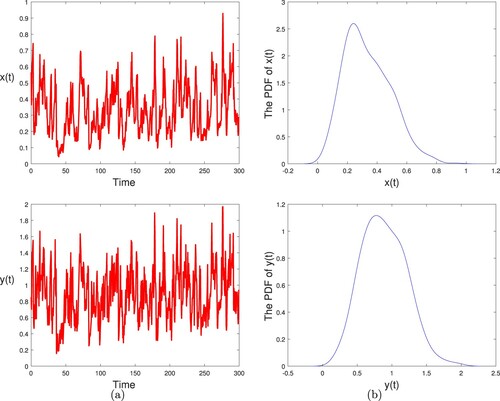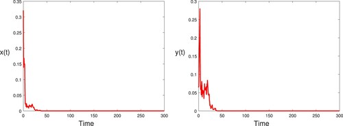2) ) has a unique stationary distribution. As seen in Figure 1, our simulation supports these results. Moreover, the sample mean and variance of $x_t$ are 0.3360 and 0.0237, and the sample mean and variance of $y_t$ are 0.8856 and 0.1022, respectively.

Figure 1. (a) The paths of $x_t$ and $y_t$ for stochastic model (2(2) $\left\{\begin{array}{l}\mathrm{d}{x}_t=\left[x_t(a_{r\left(t\right)}-b_{r\left(t\right)}{x}_t)-m_{1_{r\left(t\right)}}{x}_t+m_{2_{r\left(t\right)}}{y}_t-E_{1_{r\left(t\right)}}{x}_t\right]\mathrm{d}t+{\sigma }_{r\left(t\right)}{x}_t\mathrm{d}{B}_t,\\ \mathrm{d}{y}_t=\left[y_t(a_{r\left(t\right)}-b_{r\left(t\right)}{y}_t)-m_{2_{r\left(t\right)}}{y}_t+m_{1_{r\left(t\right)}}{x}_t-E_{2_{r\left(t\right)}}{y}_t\right]\mathrm{d}t+{\sigma }_{r\left(t\right)}{y}_t\mathrm{d}{B}_t,\end{array}\right.$(2) ) with initial values $(x_0,y_0,r(0\left)\right)=(1,2,1)$. (b) The probability density function (PDF) of $x_t$ and $y_t$, respectively. The parameter values are given in (15(15) $b_1=b_2,m_{1_1}=m_{1_2},m_{2_1}=m_{2_2},E_{1_1}=E_{1_2},E_{2_1}=E_{2_2},{\sigma }_1={\sigma }_2.$(15) ) and (16(16) $a_1=0.9,a_2=0.3,b_1=0.8,m_{1_1}=0.4,m_{2_1}=0.1,E_{1_1}=0.3,E_{2_1}=0.01,{\sigma }_1=\mathrm{0.3.}$(16) ).

As shown in [31], poaching is a major threat to the long-term persistence of the endangered species. In fact, if below some critical population density, someone is always willing to pay enough to offset the costs of finding and hunting the species, hunting further reduces the population, which increases the price of a unit harvest, which in turn increases the hunting effort, and the species is driven into an extinction vortex. Next we focus on the effects of the intensity of poaching on the single species population dynamics for model (2(2) $\left\{\begin{array}{l}\mathrm{d}{x}_t=\left[x_t(a_{r\left(t\right)}-b_{r\left(t\right)}{x}_t)-m_{1_{r\left(t\right)}}{x}_t+m_{2_{r\left(t\right)}}{y}_t-E_{1_{r\left(t\right)}}{x}_t\right]\mathrm{d}t+{\sigma }_{r\left(t\right)}{x}_t\mathrm{d}{B}_t,\\ \mathrm{d}{y}_t=\left[y_t(a_{r\left(t\right)}-b_{r\left(t\right)}{y}_t)-m_{2_{r\left(t\right)}}{y}_t+m_{1_{r\left(t\right)}}{x}_t-E_{2_{r\left(t\right)}}{y}_t\right]\mathrm{d}t+{\sigma }_{r\left(t\right)}{y}_t\mathrm{d}{B}_t,\end{array}\right.$(2) ). we carry out the following example.

Example 5.2

Based on Example 5.1, we use different vector fields values of $E_1=(E_{1_1},E_{1_2})$ and $E_2=(E_{2_1},E_{2_2})$ to investigate the effect of the poaching on the survival of population. We then divide our simulations into two cases:

Case 1.

$E_1=(0.32,0.32)$, $E_2=(0.3,0.3)$. And straightforward calculation shows $\sum _{i=1}^2{\pi }_i[a_i-\frac{{\sigma }_i^2}{2}-E_{1_i}-m_{1_i}]=0.015>0$, $\sum _{i=1}^2{\pi }_i[a_i-\frac{{\sigma }_i^2}{2}-E_{2_i}-m_{2_i}]=0.3350>0$, $\sum _{i=1}^2{\pi }_i{\lambda }_i=0.1375>0$. By Theorems 3.2 (ii) and 3.3, one can get that the single species in the nature reserve and the natural environment are always persistent in mean, and the hybrid system (2(2) $\left\{\begin{array}{l}\mathrm{d}{x}_t=\left[x_t(a_{r\left(t\right)}-b_{r\left(t\right)}{x}_t)-m_{1_{r\left(t\right)}}{x}_t+m_{2_{r\left(t\right)}}{y}_t-E_{1_{r\left(t\right)}}{x}_t\right]\mathrm{d}t+{\sigma }_{r\left(t\right)}{x}_t\mathrm{d}{B}_t,\\ \mathrm{d}{y}_t=\left[y_t(a_{r\left(t\right)}-b_{r\left(t\right)}{y}_t)-m_{2_{r\left(t\right)}}{y}_t+m_{1_{r\left(t\right)}}{x}_t-E_{2_{r\left(t\right)}}{y}_t\right]\mathrm{d}t+{\sigma }_{r\left(t\right)}{y}_t\mathrm{d}{B}_t,\end{array}\right.$(2) ) has a unique stationary distribution. The sample mean and variance of $x_t$ are 0.2565 and 0.0186, and the sample mean and variance of $y_t$ are 0.5647 and 0.0638, respectively (see Figure 2). In addition, we also plot the component-wise sample paths of $x_t$ and $y_t$ in Figure 3. In Figure 3, the blue line, green line and red line represent the sample paths of $x_t$, $y_t$ when there is only one state $r\left(t\right)=1$, $r\left(t\right)=2$ and switching back and forth from one state $r\left(t\right)=1$ to another state $r\left(t\right)=2$, respectively. It is clear that the red line is higher than the blue line, but almost all are lower than the green line. More specifically, the single species is stochastic persistent for state 1 and the hybrid system, and for state 2 it is extinct.

Case 2.

$E_1=(0.82,0.82)$, $E_2=(0.8,0.8)$. Similarly, we have $\sum _{i=1}^2{\pi }_i[a_i-\frac{{\sigma }_i^2}{2}-E_{2_i}]=-0.065<0$. By Theorems 3.2 (i), one can see that the single species in the nature reserve and the natural environment are always extinct (see Figure 5).

Figure 2. (a) The paths of $x_t$ and $y_t$ for stochastic model (2(2) $\left\{\begin{array}{l}\mathrm{d}{x}_t=\left[x_t(a_{r\left(t\right)}-b_{r\left(t\right)}{x}_t)-m_{1_{r\left(t\right)}}{x}_t+m_{2_{r\left(t\right)}}{y}_t-E_{1_{r\left(t\right)}}{x}_t\right]\mathrm{d}t+{\sigma }_{r\left(t\right)}{x}_t\mathrm{d}{B}_t,\\ \mathrm{d}{y}_t=\left[y_t(a_{r\left(t\right)}-b_{r\left(t\right)}{y}_t)-m_{2_{r\left(t\right)}}{y}_t+m_{1_{r\left(t\right)}}{x}_t-E_{2_{r\left(t\right)}}{y}_t\right]\mathrm{d}t+{\sigma }_{r\left(t\right)}{y}_t\mathrm{d}{B}_t,\end{array}\right.$(2) ) with initial values $(x_0,y_0,r(0\left)\right)=(1,2,1)$. (b) The probability density function (PDF) of $x_t$ and $y_t$, respectively. Here $E_{1_1}=E_{1_2}=0.32$, $E_{2_1}=E_{2_2}=0.3$, other parameter values are given in (15(15) $b_1=b_2,m_{1_1}=m_{1_2},m_{2_1}=m_{2_2},E_{1_1}=E_{1_2},E_{2_1}=E_{2_2},{\sigma }_1={\sigma }_2.$(15) ) and (16(16) $a_1=0.9,a_2=0.3,b_1=0.8,m_{1_1}=0.4,m_{2_1}=0.1,E_{1_1}=0.3,E_{2_1}=0.01,{\sigma }_1=\mathrm{0.3.}$(16) ).

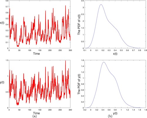
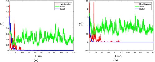
Figure 3. (a) The red line, green line and blue line represent the paths of $x_t$ for hybrid system, state 1 and state 2, respectively. (b) The red line, green line and blue line represent the paths of $y_t$ for hybrid system, state 1 and state 2, respectively. Here the parameters take the same values as in Figure 2.

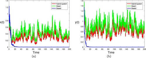
Figure 4. The evolution of $x_t$ and $y_t$ of the stochastic model (2(2) $\left\{\begin{array}{l}\mathrm{d}{x}_t=\left[x_t(a_{r\left(t\right)}-b_{r\left(t\right)}{x}_t)-m_{1_{r\left(t\right)}}{x}_t+m_{2_{r\left(t\right)}}{y}_t-E_{1_{r\left(t\right)}}{x}_t\right]\mathrm{d}t+{\sigma }_{r\left(t\right)}{x}_t\mathrm{d}{B}_t,\\ \mathrm{d}{y}_t=\left[y_t(a_{r\left(t\right)}-b_{r\left(t\right)}{y}_t)-m_{2_{r\left(t\right)}}{y}_t+m_{1_{r\left(t\right)}}{x}_t-E_{2_{r\left(t\right)}}{y}_t\right]\mathrm{d}t+{\sigma }_{r\left(t\right)}{y}_t\mathrm{d}{B}_t,\end{array}\right.$(2) ) is graphed for vield fields $(E_1,E_2)=(0.3,0.01)$, $(E_1,E_2)=(0.32,0.3)$, $(E_1,E_2)=(0.82,0.8)$. Other parameter values are given in (15(15) $b_1=b_2,m_{1_1}=m_{1_2},m_{2_1}=m_{2_2},E_{1_1}=E_{1_2},E_{2_1}=E_{2_2},{\sigma }_1={\sigma }_2.$(15) ) and (16(16) $a_1=0.9,a_2=0.3,b_1=0.8,m_{1_1}=0.4,m_{2_1}=0.1,E_{1_1}=0.3,E_{2_1}=0.01,{\sigma }_1=\mathrm{0.3.}$(16) ).

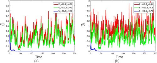
Figure 5. The paths of $x_t$ and $y_t$ for stochastic model (2(2) $\left\{\begin{array}{l}\mathrm{d}{x}_t=\left[x_t(a_{r\left(t\right)}-b_{r\left(t\right)}{x}_t)-m_{1_{r\left(t\right)}}{x}_t+m_{2_{r\left(t\right)}}{y}_t-E_{1_{r\left(t\right)}}{x}_t\right]\mathrm{d}t+{\sigma }_{r\left(t\right)}{x}_t\mathrm{d}{B}_t,\\ \mathrm{d}{y}_t=\left[y_t(a_{r\left(t\right)}-b_{r\left(t\right)}{y}_t)-m_{2_{r\left(t\right)}}{y}_t+m_{1_{r\left(t\right)}}{x}_t-E_{2_{r\left(t\right)}}{y}_t\right]\mathrm{d}t+{\sigma }_{r\left(t\right)}{y}_t\mathrm{d}{B}_t,\end{array}\right.$(2) ) with initial values $(x_0,y_0,r(0\left)\right)=(1,2,1)$. Here $E_{1_1}=E_{1_2}=0.82$, $E_{2_1}=E_{2_2}=0.8$, other parameter values are given in (15(15) $b_1=b_2,m_{1_1}=m_{1_2},m_{2_1}=m_{2_2},E_{1_1}=E_{1_2},E_{2_1}=E_{2_2},{\sigma }_1={\sigma }_2.$(15) ) and (16(16) $a_1=0.9,a_2=0.3,b_1=0.8,m_{1_1}=0.4,m_{2_1}=0.1,E_{1_1}=0.3,E_{2_1}=0.01,{\sigma }_1=\mathrm{0.3.}$(16) ).

As the intensity of poaching $E_1$ and $E_2$ increases, the hybrid system changes from stochastic permanence to extinction (see Figure 4). In other words, poaching has great influence on the survival of species.

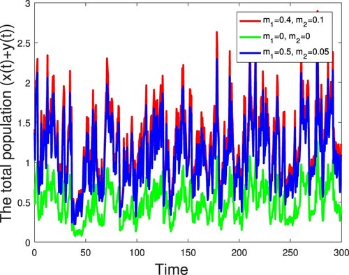
Next, we will investigate the effective ways mentioned in [31], which is increasing the migration rate $m_1$ and decreasing migration rate $m_2$ simultaneously, to protect biodiversity.

Example 5.3

Based on Example 5.1, we use different vector fields values of $m_1=(m_{1_1},m_{1_2})$ and $m_2=(m_{2_1},m_{2_2})$ to investigate the effect of the poaching on the survival of population. We then divide our simulations into two cases:

Case 1.

Without protection zone, i.e. $m_1=(0,0)$, $m_2=(0,0)$. By straightforward calculation shows $\sum _{i=1}^2{\pi }_i[a_i-\frac{{\sigma }_i^2}{2}-E_i]=0.435>0$. By Corollary 3.2, one can get that the single species is persistent in mean, and the hybrid system (6(6) $\mathrm{d}{x}_t=\left[x_t(a_{r\left(t\right)}-b_{r\left(t\right)}{x}_t)-E_{r\left(t\right)}{x}_t\right]\mathrm{d}t+{\sigma }_{r\left(t\right)}{x}_t\mathrm{d}{B}_t.$(6) ) has a unique stationary distribution.

Case 2.

$m_1=(0.5,0.5)$, $m_2=(0.05,0.05)$. Results of one simulation run are reported in Figure 6. We can claim from Figure 6 that increasing the migration rate $m_1$ or decreasing the migration rate $m_2$, the density of the total population $x_t+y_t$ will increase. Therefore, establishing key protected areas and enlarging the size of protection zone, to increase the migration rate $m_1$ and decrease the migration rate $m_2$, to ensure the reproduction of species in the area is an effective way to protect biodiversity.

Figure 6. The evolution of the total population $x_t+y_t$ of the stochastic model (2(2) $\left\{\begin{array}{l}\mathrm{d}{x}_t=\left[x_t(a_{r\left(t\right)}-b_{r\left(t\right)}{x}_t)-m_{1_{r\left(t\right)}}{x}_t+m_{2_{r\left(t\right)}}{y}_t-E_{1_{r\left(t\right)}}{x}_t\right]\mathrm{d}t+{\sigma }_{r\left(t\right)}{x}_t\mathrm{d}{B}_t,\\ \mathrm{d}{y}_t=\left[y_t(a_{r\left(t\right)}-b_{r\left(t\right)}{y}_t)-m_{2_{r\left(t\right)}}{y}_t+m_{1_{r\left(t\right)}}{x}_t-E_{2_{r\left(t\right)}}{y}_t\right]\mathrm{d}t+{\sigma }_{r\left(t\right)}{y}_t\mathrm{d}{B}_t,\end{array}\right.$(2) ) is graphed for vield fields $(m_1,m_2)=(0.4,0.1)$, $(m_1,m_2)=(0,0)$, $(m_1,m_2)=(0.5,0.05)$. Other parameter values are given in (15(15) $b_1=b_2,m_{1_1}=m_{1_2},m_{2_1}=m_{2_2},E_{1_1}=E_{1_2},E_{2_1}=E_{2_2},{\sigma }_1={\sigma }_2.$(15) ) and (16(16) $a_1=0.9,a_2=0.3,b_1=0.8,m_{1_1}=0.4,m_{2_1}=0.1,E_{1_1}=0.3,E_{2_1}=0.01,{\sigma }_1=\mathrm{0.3.}$(16) ).

Example 5.4

Based on Case 1 in Example 5.2, let the generator of $r\left(t\right)$ be $\mathrm{\Gamma }=\left(\begin{array}{cc}-338& 338\\ 27& -27\end{array}\right).$ Similarly, we have $\pi =({\pi }_1,{\pi }_2)=(0.0740,0.926)$ and $\sum _{i=1}^2{\pi }_i[a_i-\frac{{\sigma }_i^2}{2}-E_{2_i}]=-0.0006<0$. By Theorem 3.2 (i), one can see that the single species in the nature reserve and the natural environment are always extinct (see Figure 7). For comparison, we plot the component-wise sample paths of $x_t$ and $y_t$ in Figure 7. From Figures 3 and 7 show that an interesting fact: if one of the subsystems is extinctive, another is stochastic persistent, then the hybrid system may be stochastic persistent if the Markov chain spends enough time in the stochastically permanent state, or vice versa. This means that Markov chain will balance the density of the population under different regimes. From biological point of view, the Markov chain $r\left(t\right)$ is conductive to the survival of species. That is to say, the Markov chain can suppress the extinction of the single species.

Figure 7. (a) The red line, green line and blue line represent the paths of $x_t$ for hybrid system, state 1 and state 2, respectively. (b) The red line, green line and blue line represent the paths of $y_t$ for hybrid system, state 1 and state 2, respectively. Here $\mathrm{\Gamma }=\left(\begin{array}{cc}-338& 338\\ 27& -27\end{array}\right),$ other parameters take the same values as in Figure 2.

We next consider the effect of the regime switching on the survival of population by use two different switching rates.

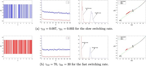
Example 5.5

To see the effect of the regime switching, we consider two different switching rates, from slow to fast. The switching rates are ${\gamma }_{12}=0.007$, ${\gamma }_{21}=0.003$ for the slow switching rate, and ${\gamma }_{12}=70$, ${\gamma }_{21}=30$ for the fast switching rate. In addition, we assume that $\sigma =0$ and other parameter sets are the same as in the Example 5.1. We have seen that for each set of parameters we get an ordinary differential equations that has a stable positive equilibrium. The upper panel shows an example of relatively slow switching. In each environmental state, the population tends to a fixed point, specific to the environment. It then fluctuates about this fixed point. The PDF is bimodal. As the switching rate is increased (lower row), the stochastic dynamics spends more time in between the two fixed points and the bimodality of the stationary distribution is lost. At fast switching, the stationary distribution becomes unimodal, peaked at a value between the two fixed points. The system spends most of its time fluctuating about a point in the interior of phase space, away from either of the two fixed points. The result is shown in Figure 8.

Figure 8. Sample paths of the dynamics and the PDF of model (2(2) $\left\{\begin{array}{l}\mathrm{d}{x}_t=\left[x_t(a_{r\left(t\right)}-b_{r\left(t\right)}{x}_t)-m_{1_{r\left(t\right)}}{x}_t+m_{2_{r\left(t\right)}}{y}_t-E_{1_{r\left(t\right)}}{x}_t\right]\mathrm{d}t+{\sigma }_{r\left(t\right)}{x}_t\mathrm{d}{B}_t,\\ \mathrm{d}{y}_t=\left[y_t(a_{r\left(t\right)}-b_{r\left(t\right)}{y}_t)-m_{2_{r\left(t\right)}}{y}_t+m_{1_{r\left(t\right)}}{x}_t-E_{2_{r\left(t\right)}}{y}_t\right]\mathrm{d}t+{\sigma }_{r\left(t\right)}{y}_t\mathrm{d}{B}_t,\end{array}\right.$(2) ) with initial values $(x_0,y_0,r(0\left)\right)=(1,2,1)$.

It is well recognized that the environment is always subject to random disturbances, so it is important to take the impact of stochastic perturbations on the evolution of the species into consideration. Next, we simulate the solution model (2(2) $\left\{\begin{array}{l}\mathrm{d}{x}_t=\left[x_t(a_{r\left(t\right)}-b_{r\left(t\right)}{x}_t)-m_{1_{r\left(t\right)}}{x}_t+m_{2_{r\left(t\right)}}{y}_t-E_{1_{r\left(t\right)}}{x}_t\right]\mathrm{d}t+{\sigma }_{r\left(t\right)}{x}_t\mathrm{d}{B}_t,\\ \mathrm{d}{y}_t=\left[y_t(a_{r\left(t\right)}-b_{r\left(t\right)}{y}_t)-m_{2_{r\left(t\right)}}{y}_t+m_{1_{r\left(t\right)}}{x}_t-E_{2_{r\left(t\right)}}{y}_t\right]\mathrm{d}t+{\sigma }_{r\left(t\right)}{y}_t\mathrm{d}{B}_t,\end{array}\right.$(2) ) with different values of σ to investigate the effect of the white noise on the survival of the species.

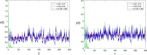
Example 5.6

To see the effect of the white noise intensity, we consider three different fields values of σ: $(0.1,0.1)$, $(0.3,0.3)$ and $(1.25,1.25)$. Other parameters take the same values as in Figure 1. By computing, we have $\sum _{i=1}^2{\pi }_i[a_i-\frac{{\sigma }_i^2}{2}-E_{1_i}-m_{1_i}]>0$, $\sum _{i=1}^2{\pi }_i[a_i-\frac{{\sigma }_i^2}{2}-E_{2_i}-m_{2_i}]>0$ in the first two cases; and $\sum _{i=1}^2{\pi }_i[a_i-\frac{{\sigma }_i^2}{2}-E_{2_i}]<0$ in the last case. It then follows from Theorem 3.2 (ii) that the single species in the nature reserve and the natural environment are always persistent in mean, in the first two cases ($\sigma =(0.1,0.1)$ and $\sigma =(0.3,0.3)$), while the single species in the nature reserve and the natural environment are always extinct in the last case (see Theorem 3.2 (i)). The computer simulations shown in Figure 9 clearly support these results. Here we can conclude that the small noise does not change the stability of the equilibrium state of model (2(2) $\left\{\begin{array}{l}\mathrm{d}{x}_t=\left[x_t(a_{r\left(t\right)}-b_{r\left(t\right)}{x}_t)-m_{1_{r\left(t\right)}}{x}_t+m_{2_{r\left(t\right)}}{y}_t-E_{1_{r\left(t\right)}}{x}_t\right]\mathrm{d}t+{\sigma }_{r\left(t\right)}{x}_t\mathrm{d}{B}_t,\\ \mathrm{d}{y}_t=\left[y_t(a_{r\left(t\right)}-b_{r\left(t\right)}{y}_t)-m_{2_{r\left(t\right)}}{y}_t+m_{1_{r\left(t\right)}}{x}_t-E_{2_{r\left(t\right)}}{y}_t\right]\mathrm{d}t+{\sigma }_{r\left(t\right)}{y}_t\mathrm{d}{B}_t,\end{array}\right.$(2) ), but with the intensity of white noise σ increasing, the volatility of $x_t$ and $y_t$ are getting larger. However when the environmental noises are relatively big, the persistence and extinction of the stochastic model (2(2) $\left\{\begin{array}{l}\mathrm{d}{x}_t=\left[x_t(a_{r\left(t\right)}-b_{r\left(t\right)}{x}_t)-m_{1_{r\left(t\right)}}{x}_t+m_{2_{r\left(t\right)}}{y}_t-E_{1_{r\left(t\right)}}{x}_t\right]\mathrm{d}t+{\sigma }_{r\left(t\right)}{x}_t\mathrm{d}{B}_t,\\ \mathrm{d}{y}_t=\left[y_t(a_{r\left(t\right)}-b_{r\left(t\right)}{y}_t)-m_{2_{r\left(t\right)}}{y}_t+m_{1_{r\left(t\right)}}{x}_t-E_{2_{r\left(t\right)}}{y}_t\right]\mathrm{d}t+{\sigma }_{r\left(t\right)}{y}_t\mathrm{d}{B}_t,\end{array}\right.$(2) ) may be affected significantly.

Figure 9. The evolution of infected individuals of stochastic model (2(2) $\left\{\begin{array}{l}\mathrm{d}{x}_t=\left[x_t(a_{r\left(t\right)}-b_{r\left(t\right)}{x}_t)-m_{1_{r\left(t\right)}}{x}_t+m_{2_{r\left(t\right)}}{y}_t-E_{1_{r\left(t\right)}}{x}_t\right]\mathrm{d}t+{\sigma }_{r\left(t\right)}{x}_t\mathrm{d}{B}_t,\\ \mathrm{d}{y}_t=\left[y_t(a_{r\left(t\right)}-b_{r\left(t\right)}{y}_t)-m_{2_{r\left(t\right)}}{y}_t+m_{1_{r\left(t\right)}}{x}_t-E_{2_{r\left(t\right)}}{y}_t\right]\mathrm{d}t+{\sigma }_{r\left(t\right)}{y}_t\mathrm{d}{B}_t,\end{array}\right.$(2) ) is graphed for $\sigma =$ $(0.1,0.1)$, $(0.3,0.3)$ and $(1.25,1.25)$. Other parameters take the same values as in Figure 1.

6. Discussion and conclusion

This article formulates a stochastic single-species model with regime switching and the impact of poaching. We first proved the existence of global positive solution. Then we investigated the extinction, persistence in mean. Moreover, we discussed the positive recurrence. Finally, numerical simulations were given in Section 5. Our investigation shows that the poaching, Markov chain, and white noise may cause great influence on the survival of species as follows:

• Poaching had a large impact on the single-species viability. As the intensity and extent of poaching increases, the odds of being at risk of extinction increases for the single species. Increasing the criminal cost of poaching is an important way to effectively protect biodiversity.

• The Markov chain $r\left(t\right)$ can suppress the extinction of the single species. Due to the hybrid system switching among different states, the species can get more chance to survival. That is to say, the larger probability of hybrid system switching to one good state, the greater the probability of survival. On the other hand, if only part of state is extinctive, the hybrid system still may be stochastically permanent, provided the Markov chain $r\left(t\right)$ spend enough time in good states (see Figures 3 and 7). From the point of view of ecology, the Markov chain $r\left(t\right)$ is beneficial for the survival of species. In other words, the Markov chain can suppress the extinction of the single species.

• The white noise, if which is relatively small, cannot change the persistence of the biological populations. However, when the white noise is relatively big, the persistence and extinction of stochastic model (2(2) $\left\{\begin{array}{l}\mathrm{d}{x}_t=\left[x_t(a_{r\left(t\right)}-b_{r\left(t\right)}{x}_t)-m_{1_{r\left(t\right)}}{x}_t+m_{2_{r\left(t\right)}}{y}_t-E_{1_{r\left(t\right)}}{x}_t\right]\mathrm{d}t+{\sigma }_{r\left(t\right)}{x}_t\mathrm{d}{B}_t,\\ \mathrm{d}{y}_t=\left[y_t(a_{r\left(t\right)}-b_{r\left(t\right)}{y}_t)-m_{2_{r\left(t\right)}}{y}_t+m_{1_{r\left(t\right)}}{x}_t-E_{2_{r\left(t\right)}}{y}_t\right]\mathrm{d}t+{\sigma }_{r\left(t\right)}{y}_t\mathrm{d}{B}_t,\end{array}\right.$(2) ) may be affected significantly.

• From a management perspective, we can protect the biodiversity of a certain area through the following strategies:

  1. Reduce the intensity of poaching $E_1$ and $E_2$ by increasing the criminal cost of poaching.

  2. Establishing key protected areas and enlarging the size of protection zone, to increase the migration rate $m_1$ and decrease the migration rate $m_2$.

At the same time, some interesting questions deserve further investigation. One may propose more realistic but complex models, such as incorporating the time delay into the system due to the time-delay environmentally fluctuating stochastic single species system exhibits an altogether different dynamical picture from model (2(2) $\left\{\begin{array}{l}\mathrm{d}{x}_t=\left[x_t(a_{r\left(t\right)}-b_{r\left(t\right)}{x}_t)-m_{1_{r\left(t\right)}}{x}_t+m_{2_{r\left(t\right)}}{y}_t-E_{1_{r\left(t\right)}}{x}_t\right]\mathrm{d}t+{\sigma }_{r\left(t\right)}{x}_t\mathrm{d}{B}_t,\\ \mathrm{d}{y}_t=\left[y_t(a_{r\left(t\right)}-b_{r\left(t\right)}{y}_t)-m_{2_{r\left(t\right)}}{y}_t+m_{1_{r\left(t\right)}}{x}_t-E_{2_{r\left(t\right)}}{y}_t\right]\mathrm{d}t+{\sigma }_{r\left(t\right)}{y}_t\mathrm{d}{B}_t,\end{array}\right.$(2) ). We leave this for future consideration.

Acknowledgements

This project was supported by the National Natural Science Foundation of China (No. 12001186), the Science Research Fund of Hunan Province Education Department (No. 20B158) and the Postgraduate Scientific Research Innovation Project of Hunan Province (No. CX20200466).

Disclosure statement

No potential conflict of interest was reported by the author(s).

Additional information

Funding

This project was supported by the National Natural Science Foundation of China [grant number 12001186], the Science Research Fund of Hunan Province Education Department [grant number 20B158] and the Postgraduate Scientific Research Innovation Project of Hunan Province [grant number CX20200466].

The proof of Corollary 3.1

Proof.

Denote $\begin{array}{r}V=x+y,\end{array}$ then from system (2(2) $\left\{\begin{array}{l}\mathrm{d}{x}_t=\left[x_t(a_{r\left(t\right)}-b_{r\left(t\right)}{x}_t)-m_{1_{r\left(t\right)}}{x}_t+m_{2_{r\left(t\right)}}{y}_t-E_{1_{r\left(t\right)}}{x}_t\right]\mathrm{d}t+{\sigma }_{r\left(t\right)}{x}_t\mathrm{d}{B}_t,\\ \mathrm{d}{y}_t=\left[y_t(a_{r\left(t\right)}-b_{r\left(t\right)}{y}_t)-m_{2_{r\left(t\right)}}{y}_t+m_{1_{r\left(t\right)}}{x}_t-E_{2_{r\left(t\right)}}{y}_t\right]\mathrm{d}t+{\sigma }_{r\left(t\right)}{y}_t\mathrm{d}{B}_t,\end{array}\right.$(2) ), we can obtain $\begin{array}{rl}\mathrm{d}V=& \left[a_{r\left(t\right)}(x+y)-b_{r\left(t\right)}{x}^2-b_{r\left(t\right)}{y}^2-E_{1_{r\left(t\right)}}x-E_{2_{r\left(t\right)}}y\right]\mathrm{d}t+{\sigma }_{r\left(t\right)}(x+y)\mathrm{d}{B}_t\\ \le & \left[M-E_{2_{r\left(t\right)}}(x+y)\right]\mathrm{d}t+{\sigma }_{r\left(t\right)}(x+y)\mathrm{d}{B}_t\\ \le & \left[M-\widehat{E_2}(x+y)\right]\mathrm{d}t+{\sigma }_{r\left(t\right)}(x+y)\mathrm{d}{B}_t,\end{array}$ where $M=max\left\{a_{r\left(t\right)}\right(x+y)-b_{r\left(t\right)}{x}^2-b_{r\left(t\right)}{y}^2\}$ for $\mathrm{\forall }r\left(t\right)\in \mathbb{S}$. In addition, we have applied the hypotheses $E_{2_{r\left(t\right)}}<E_{1_{r\left(t\right)}}$ for $\mathrm{\forall }r\left(t\right)\in \mathbb{S}$ in here. Now consider the following equation $\left\{\begin{array}{l}dY=(A-\widehat{E_2}Y)\mathrm{d}t+{\sigma }_{r\left(t\right)}(x+y)\mathrm{d}{B}_t,\\ Y_0=x_0+y_0.\end{array}\right.$ By Theorem 3.9 in [23], we have $\underset{t\to \mathrm{\infty }}{lim}Y\left(t\right)<\mathrm{\infty }$ almost surely. Then according to the comparison theorem for stochastic differential equations, this yields $\begin{array}{r}\underset{t\to \mathrm{\infty }}{lim sup}(x_t+y_t)<\mathrm{\infty }\mathrm{a}.\mathrm{s}.\end{array}$ According to Theorem 3.1, for any initial value $(x_0,y_0,r(0\left)\right)\in {\mathbb{R}}_{+}^2\times \mathbb{S}$, we have $x_t\ge 0\text{ and }{y}_t\ge 0\text{ a.s.}$ which implies that $\underset{t\to \mathrm{\infty }}{lim sup}\frac{\ln x_t}{t}=0\mathrm{a}\mathrm{n}\mathrm{d}\underset{t\to \mathrm{\infty }}{lim sup}\frac{\ln x_t}{t}=0,\mathrm{a}.\mathrm{s}.$ This completes the proof.

References

- R. Alley, J. Marotzke and W. Nordhaus, et al. Abrupt climate change, Science 299 (2003), pp. 2005–2010.
- M. Assaf, A. Kamenev and B. Meerson, Population extinction risk in the aftermath of a catastrophic event, Phys. Rev. E79 (2009), pp. 011127.
- H. Bauer, G. Chapron, K. Nowell and et al, Lion (Pantheraleo) populations are declining rapidly across Africa except in intensively managed areas, Proc. Natl. Acad. Sci. 112 (2015), pp. 14894–14899.
- P. Berck, Open access and extinction, Econometrica 47 (1979), pp. 877–882.
- F. Berkes, D. Feeny and B. Mccay, et al. The benefits of the commons, Nature 340 (1989), pp. 91–93.
- J. Blanco, S. Reig and L. De-La-Cuesta, Distribution status and conservation problems of the wolf Canis lupus in Spain, Biol. Conserv. 60 (1992), pp. 73–80.
- U. Breitenmoser, C. Breitenmoser-Würsten and S. Capt, et al. Conservation of the lynx Lynx lynx in the Swiss Jura Mountains, Wildlife Biol. 13 (2007), pp. 340–355.
- E. Bulte, H. Folmer and W. Heijman, Open access common property and scarcity rent in fisheries, Environ. Resour. Econ. 6 (1995), pp. 309–320.
- F. Courchamp, E. Angulo and P. Rivalan, et al. Rarity value and species extinction: the anthropogenic Allee effect, PLoS Biol. 4 (2006), pp. e415.
- B. Dubey, P. Chandra and P. Sinha, A model for fishery resource with reserve area, Nonlin. Anal. Real 4 (2003), pp. 625–637.
- T. Gard, Persistence in stochastic food web models, Bull.Math. Biol. 46 (1984), pp. 357–370.
- T. Gard, Stability for multispecies population models in random environments, Nonlin. Anal. 10 (1986), pp. 1411–1419.
- R. Hall, E. Milner-Gulland and F. Courchamp, Endangering the endangered: the effects of perceived rarity on species exploitation, Conserv. Lett. 1 (2008), pp. 75–81.
- L. Hu, M. Huang and M. Tang, et al. Wolbachia spread dynamics in stochastic environments, Theor. Popul. Biol. 106 (2015), pp. 32–44.
- L. Hu, M. Huang and M. Tang, et al. Wolbachia spread dynamics in multi-regimes of environmental conditions, J. Theor. Biol. 462 (2019), pp. 247–258.
- L. Hu, M. Tang and Z. Wu, et al. The threshold infection level for wolbachia invasion in random environments, J. Differ. Equ. 266 (2019), pp. 4377–4393.
- T. Kar and H. Matsuda, A bioeconomic model of a single-species fishery with a marine reserve, J. Environ. Manag. 86 (2008), pp. 171–180.
- R. Khasminskii, C. Zhu and G. Yin, Stability of regime-switching diffusions, Stoch. Proc. Appl. 117 (2007), pp. 1037–1051.
- J. Kenney, J. Smith and A. Starfield, et al. The long-term effects of tiger poaching on population viability, Conserv. Biol. 9 (1995), pp. 1127–1133.
- G. Lan, Z. Lin, C. Wei and S. Zhang, A stochastic SIRS epidemic model with non-monotone incidence rate under regime-switching, J. Frankl. Inst. 356 (2019), pp. 9844–9866.
- M. Liu, X. He and J. Yu, Dynamics of a stochastic regime-switching predator-prey model with harvesting and distributed delays, Nonlin. Anal. Hybrid. 28 (2018), pp. 87–104.
- M. Liu, W. Li and K. Wang, Persistence and extinction of a stochastic delay logistic equation under regime switching, Appl. Math. Lett. 26 (2013), pp. 140–144.
- X. Mao, Stochastic Differential Equations and Applications, Horwood Publishing, Chichester, 1997.
- R. May, Stability and Complexity in Model Ecosystems, Princeton University Press, Princeton, 2001.
- X. Mao and C. Yuan, Stochastic Differential Equations with Markovian Switching, Imperial College Press, London, 2006.
- W. Ripple, J. Estes and R. Beschta, et al. Status and ecological effects of the world's largest carnivores, Science343 (2014), pp. 1241484.
- J. Seidensticker, Saving wild tigers: a case study in biodiversity loss and challenges to be met for recovery beyond 2010, Integr. Zool. 5 (2010), pp. 285–299.
- M. Scheffer and S. Carpenter, Catastrophic regime shifts in ecosystems: linking theory to observation, Trends Ecol. Evol. 12 (2003), pp. 648–656.
- M. Scheffer, S. Carpenter and J. Foley, et al. Catastrophic shifts in ecosystems, Nature 413 (2001), pp. 591–596.
- M. Slatkin, The dynamics of a population in a Markovian environment, Ecol. 59 (1978), pp. 249–256.
- F. Wei and C. Wang, Survival analysis of a single-species population model with fluctuations and migrations between patches, Appl. Math. Model. 81 (2020), pp. 113–127.
- G. Yin and C. Zhu, Asymptotic properties of hybrid diffusion systems, SIAM J. Control Optim. 46 (2007), pp. 1155–1179.
- X. Yu, S. Yuan and T. Zhang, Persistence and ergodicity of a stochastic single species model with allee effect under regime switching, Commun. Nonlin. Sci. Numer. Simul. 59 (2018), pp. 359–374.
- Y. Zhao, S. Yuan and T. Zhang, The stationary distribution and ergodicity of a stochastic phytoplankton allelopathy model under regime switching, Commun. Nonlin. Sci. Numer. Simul. 37 (2016), pp. 131–142.
- X. Zou and K. Wang, A robustness analysis of biological population models with protection zone, Appl. Math. Model. 35 (2011), pp. 5553–5563.
- X. Zou and K. Wang, Dynamical properties of biological population with a protected area under ecological uncertainty, Appl. Math. Model. 39 (2015), pp. 6273–6284.