Long-term transmission dynamics of tick-borne diseases involving seasonal variation and co-feeding transmission

Abstract

Co-feeding is a mode of pathogen transmission for a wide range of tick-borne diseases where susceptible ticks can acquire infection from co-feeding with infected ticks on the same hosts. The significance of this transmission pathway is determined by the co-occurrence of ticks at different stages in the same season. Taking this into account, we formulate a system of differential equations with tick population dynamics and pathogen transmission dynamics highly regulated by the seasonal temperature variations. We examine the global dynamics of the model systems, and show that the two important ecological and epidemiological basic reproduction numbers can be used to fully characterize the long-term dynamics, and we link these two important threshold values to efficacy of co-feeding transmission.

Keywords:

• Co-feeding transmission
• tick-borne disease dynamics
• periodic system of differential equations

1. Introduction

Incidences of tick-borne diseases (TBDs) such as Lyme disease or tick-borne encephalitis (TBE) have significantly increased in several parts of Europe and North America in the past decades. Climate conditions influence the transmission risk of TBDs since the life cycle of ticks depends on abiotic factors such as temperature, daylight length and humidity as well as biotic factors, for example the host abundance [1,2].

The TBD pathogens are delivered to a susceptible host during the blood-feeding of infected ticks. When this provokes a systemic infection in the host, susceptible ticks can subsequently get infected as they feed the infected host [26]. Recent discoveries suggest that pathogens may also be transmitted between co-feeding infected and uninfected ticks in the absence of the pathogen being established in the host [27,34]. This co-feeding transmission generally occurs between infected nymphs and susceptible larvae [26,34]. The significance of this mode of transmission depends on whether ticks in larval and nymphal stages are active in the same seasons of the year [26]. Co-feeding transmission is reported for many types of vector-borne pathogens and bridging hosts [6,27,34]. In particular, it is shown that Ixodes ricinis, a native European tick can efficiently transmit TBE virus and Lyme Borrelia bacterium via non-viraemic hosts [6,13].

The co-feeding transmission pathway is considered to enhance the transmission risk. Unlike systemic transmission, non-systemic transmission may occur immediately after the infectious tick taking blood meal and it dampens reduction of the transmission potential induced by natural mortality of hosts. In addition, more types of hosts involved in the disease transmission since some hosts which do not develop systemic infection can still serve as bridges for the co-feeding transmission [27]. Moreover, co-feeding transmission is observed in the hosts with immunity resulting in the increase of the number of transmission-competent hosts [14,26,27].

Several studies adapted a structured compartmental model as a framework to study the population dynamics of ticks and TBDs [5,18]. A basic reproduction number $R_0$, a local stability threshold of such a dynamical system is often used to inform the risk factors [33]. Norman et al. [20] and Rosà and Pugliese [30] studied the effect of the host population structure and their densities on the tick population growth or TBD by identifying $R_0$s of both the tick population and TBD transmission dynamics. Similarly, White at al. [36] studied a condition for the coexistence of two pathogens and Lou at al. [17] investigated how co-infection changes the fitness of pathogens.

In order to gain insights on which factors more significantly affect the long-term behaviours of tick population dynamics or the infection dynamics, some studied the stability or persistence in models for multistage populations [3,4,8,10,16,37,39]. Zhang and Wu [39] studied how the vector attachment and host grooming lead to bi-stability and nonlinear oscillations in the tick populations. Fan et al. [3] showed that a negative feedback from feeding to egg-laying adults leads to oscillations of tick population. A few studies qualitatively examined tick population or TBE transmission dynamics in a seasonal environment. For example, Lou et al. [16] and Wu and Wu [37] studied periodic systems describing population dynamics of ticks and TBD spread using the theory of monotone dynamical systems.

Some of the theoretical modelling studies included the co-feeding transmission in their models [7,21,31,36,38,40]. Using the pathogen basic reproduction number, Rosà et al. [31] showed that a co-feeding transmission enables the disease to persist even when hosts do not acquire and transmit the disease systemically. A similar result was obtained in [21]. In addition, some studies showed that co-feeding transmission increases the basic reproduction number or the prevalence in the study regions [19,28].

In this paper, we study the global dynamics of a proposed periodic system of ordinary differential equations describing the transmission of pathogens between ticks and hosts. The basic reproduction numbers for tick population growth and TBD spread are defined, and we will show that these two basic reproduction numbers determine the global long-term behaviours of solutions. We also perform some numerical simulations to see how co-feeding transmission changes the asymptotic behaviours of epidemiological system.

2. Models

2.1. Tick population dynamics

We first introduce a model describing the dynamics of tick populations in various life stages: eggs (E), questing larvae ($L_q$), feeding larvae ($L_f$), questing nymphs ($L_q$), feeding nymphs ($L_f$), questing adults ($A_q$), feeding adults ($A_f$). Ticks in questing stages ($L_q$, $N_q$, $A_q$) move to feeding stages with the host-attaching rates ${\alpha }_l\left(t\right)$, ${\alpha }_n\left(t\right)$ and ${\alpha }_a\left(t\right)$. Upon successful blood feeding, adult ticks will reproduce eggs with the rate $b\left(t\right)$, while larval and nymphal ticks develop into the next stages with the development rates $d_l\left(t\right)$ and $d_n\left(t\right)$.

The mortality of ticks attached to hosts is density-dependent due to host immunity and grooming behaviours [15,25]. As in other modelling studies [17,22,37], we assume that ticks in each feeding stage experience density-dependent mortalities which is increasing with the number feeding ticks in the same stage. As an example, the mortality of feeding larvae is an increasing function of the average number of feeding larvae per host ($L_f/H$). Questing ticks and eggs are assumed to undergo density-independent, constant mortality rates. Accounting for the seasonal dependence of the parameters, we describe the tick population dynamics with the following non-autonomous system of ordinary differential equations, (1) $\left\{\begin{array}{ll}{L}_q^{\prime }& =d_e\left(t\right)E-{\alpha }_l\left(t\right)L_q-{\mu }_{ql}{L}_q,\\ L_f^{\prime }& ={\alpha }_l\left(t\right)L_q-d_l\left(t\right)L_f-{\mu }_{fl}\left(\frac{L_f}{H}\right)L_f,\\ N_q^{\prime }& =d_l\left(t\right)L_f-{\alpha }_n\left(t\right)N_q-{\mu }_{qn}{N}_q,\\ N_f^{\prime }& ={\alpha }_n\left(t\right)N_q-d_n\left(t\right)N_f-{\mu }_{fn}\left(\frac{N_f}{H}\right)N_f,\\ A_q^{\prime }& =d_n\left(t\right)N_f-{\alpha }_a\left(t\right)A_q-{\mu }_{qa}{A}_q,\\ A_f^{\prime }& ={\alpha }_a\left(t\right)A_q-{\mu }_{fa}\left(\frac{A_f}{H}\right)A_f,\\ E^{\prime }& =b\left(t\right)A_f-d_e\left(t\right)E-{\mu }_{e}E,\end{array}\right.$(1) where parameters are positive, bounded, p-periodic and the density-dependent mortalities ${\mu }_{fl}(\cdot )$, ${\mu }_{fn}(\cdot )$ and ${\mu }_{fa}(\cdot )$ are strictly increasing and continuously differentiable functions.

The tick population growth model with the same structure is studied in previous works and a proof of the following lemma can be found in paper [37].

Lemma 2.1

The system (1(1) $\left\{\begin{array}{ll}{L}_q^{\prime }& =d_e\left(t\right)E-{\alpha }_l\left(t\right)L_q-{\mu }_{ql}{L}_q,\\ L_f^{\prime }& ={\alpha }_l\left(t\right)L_q-d_l\left(t\right)L_f-{\mu }_{fl}\left(\frac{L_f}{H}\right)L_f,\\ N_q^{\prime }& =d_l\left(t\right)L_f-{\alpha }_n\left(t\right)N_q-{\mu }_{qn}{N}_q,\\ N_f^{\prime }& ={\alpha }_n\left(t\right)N_q-d_n\left(t\right)N_f-{\mu }_{fn}\left(\frac{N_f}{H}\right)N_f,\\ A_q^{\prime }& =d_n\left(t\right)N_f-{\alpha }_a\left(t\right)A_q-{\mu }_{qa}{A}_q,\\ A_f^{\prime }& ={\alpha }_a\left(t\right)A_q-{\mu }_{fa}\left(\frac{A_f}{H}\right)A_f,\\ E^{\prime }& =b\left(t\right)A_f-d_e\left(t\right)E-{\mu }_{e}E,\end{array}\right.$(1) ) has a unique, non-negative and bounded solution for each initial value in ${\mathbb{R}}_{+}^7$.

2.2. Disease transmission dynamics

We divide the tick and host population into those which are susceptible and infectious to TBD, with subscript ‘s’ and ‘i’, respectively. All questing larvae are considered to be susceptible. In line with this assumption, we limit our focus on the tick-borne diseases with rare transovarial transmission, such as for Lyme disease or tick-borne encephalitis [23,24]. Upon the successful attachment to an infected host, the questing larvae and susceptible questing nymphs will be infected with probabilities ${\text{β}}_{hl}$ and ${\text{β}}_{hn}$ respectively, via the systemic infection route. In addition, we consider co-feeding infection, that is, when they feed the susceptible hosts or feed on infected hosts but escapes the systemic infection, the ticks may still get infected via non-systemic transmission with a probability $\delta \left(N_{fi}/H\right)$. This probability is assumed to be increasing with respect to the average number of infected feeding nymphs per hosts. Finally, we assume that when the infected questing nymphs attach to a susceptible host, the host may be infected with a probability ${\text{β}}_{nh}$. Therefore, we obtain a system describing the spread of TBD pathogens, (2) $\left\{\begin{array}{ll}{L}_q^{\prime }& =d_e\left(t\right)E-{\alpha }_l\left(t\right)L_q-{\mu }_{ql}{L}_q,\\ L_{fs}^{\prime }& =\left(1-\delta \left(\frac{N_{fi}}{H}\right)\right){\alpha }_l\left(t\right)\left(\frac{H_s}{H}+(1-{\text{β}}_{hl})\frac{H_i}{H}\right)L_q\\ & -d_l\left(t\right)L_{fs}-{\mu }_{fl}\left(\frac{L_{fs}+L_{fi}}{H}\right)L_{fs},\\ L_{fi}^{\prime }& =\delta \left(\frac{N_{fi}}{H}\right){\alpha }_l\left(t\right)\left(\frac{H_s}{H}+(1-{\text{β}}_{hl})\frac{H_i}{H}\right)L_q+{\text{β}}_{hl}{\alpha }_l\left(t\right)\frac{H_i}{H}{L}_q\\ & -d_l\left(t\right)L_{fi}-{\mu }_{fl}\left(\frac{L_{fs}+L_{fi}}{H}\right)L_{fi},\\ N_{qs}^{\prime }& =d_l\left(t\right)L_{fs}-{\alpha }_n\left(t\right)N_{qs}-{\mu }_{qn}{N}_{qs},\\ N_{qi}^{\prime }& =d_l\left(t\right)L_{fi}-{\alpha }_n\left(t\right)N_{qi}-{\mu }_{qn}{N}_{qi},\\ N_{fs}^{\prime }& =\left(1-\delta \left(\frac{N_{fi}}{H}\right)\right){\alpha }_n\left(t\right)\left(\frac{H_s}{H}+(1-{\text{β}}_{hl})\frac{H_i}{H}\right)N_{qs}\\ & -d_n\left(t\right)N_{fs}-{\mu }_{fn}\left(\frac{N_{fs}+N_{fi}}{H}\right)N_{fs},\\ N_{fi}^{\prime }& =\delta \left(\frac{N_{fi}}{H}\right){\alpha }_n\left(t\right)\left(\frac{H_s}{H}+(1-{\text{β}}_{hn})\frac{H_i}{H}\right)N_{qs}+{\text{β}}_{hn}{\alpha }_n\left(t\right)\frac{H_i}{H}{N}_{qs}+{\alpha }_n\left(t\right)N_{qi}\\ & -d_n\left(t\right)N_{fi}-{\mu }_{fn}\left(\frac{N_{fs}+N_{fi}}{H}\right)N_{fi},\\ A_q^{\prime }& =d_n\left(t\right)(N_{fs}+N_{fi})-{\alpha }_a\left(t\right)A_q-{\mu }_{qa}{A}_q,\\ A_f^{\prime }& ={\alpha }_a\left(t\right)A_q-{\mu }_{fa}\left(\frac{A_f}{D}\right)A_f,\\ E^{\prime }& =b\left(t\right)A_f-d_e\left(t\right)E-{\mu }_{e}E,\\ H_s^{\prime }& ={\mu }_{h}H-{\text{β}}_{nh}{\alpha }_n\left(t\right)N_{qi}\frac{H_s}{H}+\gamma H_i-{\mu }_h{H}_i,\\ H_i^{\prime }& ={\text{β}}_{nh}{\alpha }_n\left(t\right)N_{qi}\frac{H_s}{H}-\gamma H_i-{\mu }_h{H}_i,\end{array}\right.$(2) where $\delta \left(x\right)=1-(1-c{)}^x$. Here, c refers to the probability of non-systemic infection for susceptible and recovered ticks attached to a host attached with a single infected nymphs. We assume that all parameters are positive, bounded, p-periodic, $0\le {\text{β}}_{hl}\le 1$, $0\le {\text{β}}_{hn}\le 1$, $0\le {\text{β}}_{nh}\le 1$ and $0\le c<1$.

Let ${\mathbb{R}}^n$ be n-dimensional vector space with Euclidean norm $|\cdot {|}_n$ and $C_r:\mathbb{R}\to {\mathbb{R}}^n$ be the Banach space of p-periodic continuous functions. For $x=(x_1,\dots ,x_n)\in {\mathbb{R}}^n$ and $y=(y_1,\dots ,y_n)\in {\mathbb{R}}^n$, we write $x\le y$ if $x_i\le y_i$ for all $i=1,\dots ,n$; x<y if $x\ne y$ and $x_i\le y_i$ for all $i=1,\dots ,n$; $x\ll y$ if $x_i<y_i$ for all $i=1,\dots ,n$. For $\varphi ,\psi \in C$, we write $\varphi \ge \psi$ if ${\varphi }_i\left(x\right)\ge {\psi }_i\left(x\right)$ for all $i\in 1,\dots ,n,x\in \mathbb{R}$; $\varphi >\psi$ if $\varphi \ge \psi$ but $\varphi \ne \psi$; $\varphi \gg \psi$ if ${\varphi }_i\left(x\right)>{\psi }_i\left(x\right)$ for all $i\in 1,\dots ,n,x\in \mathbb{R}$.

Lemma 2.2

The system (2(2) $\left\{\begin{array}{ll}{L}_q^{\prime }& =d_e\left(t\right)E-{\alpha }_l\left(t\right)L_q-{\mu }_{ql}{L}_q,\\ L_{fs}^{\prime }& =\left(1-\delta \left(\frac{N_{fi}}{H}\right)\right){\alpha }_l\left(t\right)\left(\frac{H_s}{H}+(1-{\text{β}}_{hl})\frac{H_i}{H}\right)L_q\\ & -d_l\left(t\right)L_{fs}-{\mu }_{fl}\left(\frac{L_{fs}+L_{fi}}{H}\right)L_{fs},\\ L_{fi}^{\prime }& =\delta \left(\frac{N_{fi}}{H}\right){\alpha }_l\left(t\right)\left(\frac{H_s}{H}+(1-{\text{β}}_{hl})\frac{H_i}{H}\right)L_q+{\text{β}}_{hl}{\alpha }_l\left(t\right)\frac{H_i}{H}{L}_q\\ & -d_l\left(t\right)L_{fi}-{\mu }_{fl}\left(\frac{L_{fs}+L_{fi}}{H}\right)L_{fi},\\ N_{qs}^{\prime }& =d_l\left(t\right)L_{fs}-{\alpha }_n\left(t\right)N_{qs}-{\mu }_{qn}{N}_{qs},\\ N_{qi}^{\prime }& =d_l\left(t\right)L_{fi}-{\alpha }_n\left(t\right)N_{qi}-{\mu }_{qn}{N}_{qi},\\ N_{fs}^{\prime }& =\left(1-\delta \left(\frac{N_{fi}}{H}\right)\right){\alpha }_n\left(t\right)\left(\frac{H_s}{H}+(1-{\text{β}}_{hl})\frac{H_i}{H}\right)N_{qs}\\ & -d_n\left(t\right)N_{fs}-{\mu }_{fn}\left(\frac{N_{fs}+N_{fi}}{H}\right)N_{fs},\\ N_{fi}^{\prime }& =\delta \left(\frac{N_{fi}}{H}\right){\alpha }_n\left(t\right)\left(\frac{H_s}{H}+(1-{\text{β}}_{hn})\frac{H_i}{H}\right)N_{qs}+{\text{β}}_{hn}{\alpha }_n\left(t\right)\frac{H_i}{H}{N}_{qs}+{\alpha }_n\left(t\right)N_{qi}\\ & -d_n\left(t\right)N_{fi}-{\mu }_{fn}\left(\frac{N_{fs}+N_{fi}}{H}\right)N_{fi},\\ A_q^{\prime }& =d_n\left(t\right)(N_{fs}+N_{fi})-{\alpha }_a\left(t\right)A_q-{\mu }_{qa}{A}_q,\\ A_f^{\prime }& ={\alpha }_a\left(t\right)A_q-{\mu }_{fa}\left(\frac{A_f}{D}\right)A_f,\\ E^{\prime }& =b\left(t\right)A_f-d_e\left(t\right)E-{\mu }_{e}E,\\ H_s^{\prime }& ={\mu }_{h}H-{\text{β}}_{nh}{\alpha }_n\left(t\right)N_{qi}\frac{H_s}{H}+\gamma H_i-{\mu }_h{H}_i,\\ H_i^{\prime }& ={\text{β}}_{nh}{\alpha }_n\left(t\right)N_{qi}\frac{H_s}{H}-\gamma H_i-{\mu }_h{H}_i,\end{array}\right.$(2) ) has a unique, non-negative and bounded solution with initial values in ${\mathbb{R}}_{+}^{12}$. Moreover, a feasible set $X:=\left\{\right(L_q,L_{fs},L_{fi},N_{qs},N_{qi},N_{fs},N_{fi},A_q,A_f,E,H_s,H_i)\in {\mathbb{R}}_{+}^{12}|H_s+H_i=H\}$is positively invariant.

Proof.

With the assumption that the density-dependent moralities ${\mu }_{fl}$, ${\mu }_{fn}$ and ${\mu }_{fa}$ are continuously differentiable, it is easy to show that the vector field given by the right hand side of the system (2(2) $\left\{\begin{array}{ll}{L}_q^{\prime }& =d_e\left(t\right)E-{\alpha }_l\left(t\right)L_q-{\mu }_{ql}{L}_q,\\ L_{fs}^{\prime }& =\left(1-\delta \left(\frac{N_{fi}}{H}\right)\right){\alpha }_l\left(t\right)\left(\frac{H_s}{H}+(1-{\text{β}}_{hl})\frac{H_i}{H}\right)L_q\\ & -d_l\left(t\right)L_{fs}-{\mu }_{fl}\left(\frac{L_{fs}+L_{fi}}{H}\right)L_{fs},\\ L_{fi}^{\prime }& =\delta \left(\frac{N_{fi}}{H}\right){\alpha }_l\left(t\right)\left(\frac{H_s}{H}+(1-{\text{β}}_{hl})\frac{H_i}{H}\right)L_q+{\text{β}}_{hl}{\alpha }_l\left(t\right)\frac{H_i}{H}{L}_q\\ & -d_l\left(t\right)L_{fi}-{\mu }_{fl}\left(\frac{L_{fs}+L_{fi}}{H}\right)L_{fi},\\ N_{qs}^{\prime }& =d_l\left(t\right)L_{fs}-{\alpha }_n\left(t\right)N_{qs}-{\mu }_{qn}{N}_{qs},\\ N_{qi}^{\prime }& =d_l\left(t\right)L_{fi}-{\alpha }_n\left(t\right)N_{qi}-{\mu }_{qn}{N}_{qi},\\ N_{fs}^{\prime }& =\left(1-\delta \left(\frac{N_{fi}}{H}\right)\right){\alpha }_n\left(t\right)\left(\frac{H_s}{H}+(1-{\text{β}}_{hl})\frac{H_i}{H}\right)N_{qs}\\ & -d_n\left(t\right)N_{fs}-{\mu }_{fn}\left(\frac{N_{fs}+N_{fi}}{H}\right)N_{fs},\\ N_{fi}^{\prime }& =\delta \left(\frac{N_{fi}}{H}\right){\alpha }_n\left(t\right)\left(\frac{H_s}{H}+(1-{\text{β}}_{hn})\frac{H_i}{H}\right)N_{qs}+{\text{β}}_{hn}{\alpha }_n\left(t\right)\frac{H_i}{H}{N}_{qs}+{\alpha }_n\left(t\right)N_{qi}\\ & -d_n\left(t\right)N_{fi}-{\mu }_{fn}\left(\frac{N_{fs}+N_{fi}}{H}\right)N_{fi},\\ A_q^{\prime }& =d_n\left(t\right)(N_{fs}+N_{fi})-{\alpha }_a\left(t\right)A_q-{\mu }_{qa}{A}_q,\\ A_f^{\prime }& ={\alpha }_a\left(t\right)A_q-{\mu }_{fa}\left(\frac{A_f}{D}\right)A_f,\\ E^{\prime }& =b\left(t\right)A_f-d_e\left(t\right)E-{\mu }_{e}E,\\ H_s^{\prime }& ={\mu }_{h}H-{\text{β}}_{nh}{\alpha }_n\left(t\right)N_{qi}\frac{H_s}{H}+\gamma H_i-{\mu }_h{H}_i,\\ H_i^{\prime }& ={\text{β}}_{nh}{\alpha }_n\left(t\right)N_{qi}\frac{H_s}{H}-\gamma H_i-{\mu }_h{H}_i,\end{array}\right.$(2) ) is Lipschitz continuous on the bounded subsets of ${\mathbb{R}}^{12}$. Therefore, for a given initial value in ${\mathbb{R}}^{12}$, there exists a unique solution of the system (2(2) $\left\{\begin{array}{ll}{L}_q^{\prime }& =d_e\left(t\right)E-{\alpha }_l\left(t\right)L_q-{\mu }_{ql}{L}_q,\\ L_{fs}^{\prime }& =\left(1-\delta \left(\frac{N_{fi}}{H}\right)\right){\alpha }_l\left(t\right)\left(\frac{H_s}{H}+(1-{\text{β}}_{hl})\frac{H_i}{H}\right)L_q\\ & -d_l\left(t\right)L_{fs}-{\mu }_{fl}\left(\frac{L_{fs}+L_{fi}}{H}\right)L_{fs},\\ L_{fi}^{\prime }& =\delta \left(\frac{N_{fi}}{H}\right){\alpha }_l\left(t\right)\left(\frac{H_s}{H}+(1-{\text{β}}_{hl})\frac{H_i}{H}\right)L_q+{\text{β}}_{hl}{\alpha }_l\left(t\right)\frac{H_i}{H}{L}_q\\ & -d_l\left(t\right)L_{fi}-{\mu }_{fl}\left(\frac{L_{fs}+L_{fi}}{H}\right)L_{fi},\\ N_{qs}^{\prime }& =d_l\left(t\right)L_{fs}-{\alpha }_n\left(t\right)N_{qs}-{\mu }_{qn}{N}_{qs},\\ N_{qi}^{\prime }& =d_l\left(t\right)L_{fi}-{\alpha }_n\left(t\right)N_{qi}-{\mu }_{qn}{N}_{qi},\\ N_{fs}^{\prime }& =\left(1-\delta \left(\frac{N_{fi}}{H}\right)\right){\alpha }_n\left(t\right)\left(\frac{H_s}{H}+(1-{\text{β}}_{hl})\frac{H_i}{H}\right)N_{qs}\\ & -d_n\left(t\right)N_{fs}-{\mu }_{fn}\left(\frac{N_{fs}+N_{fi}}{H}\right)N_{fs},\\ N_{fi}^{\prime }& =\delta \left(\frac{N_{fi}}{H}\right){\alpha }_n\left(t\right)\left(\frac{H_s}{H}+(1-{\text{β}}_{hn})\frac{H_i}{H}\right)N_{qs}+{\text{β}}_{hn}{\alpha }_n\left(t\right)\frac{H_i}{H}{N}_{qs}+{\alpha }_n\left(t\right)N_{qi}\\ & -d_n\left(t\right)N_{fi}-{\mu }_{fn}\left(\frac{N_{fs}+N_{fi}}{H}\right)N_{fi},\\ A_q^{\prime }& =d_n\left(t\right)(N_{fs}+N_{fi})-{\alpha }_a\left(t\right)A_q-{\mu }_{qa}{A}_q,\\ A_f^{\prime }& ={\alpha }_a\left(t\right)A_q-{\mu }_{fa}\left(\frac{A_f}{D}\right)A_f,\\ E^{\prime }& =b\left(t\right)A_f-d_e\left(t\right)E-{\mu }_{e}E,\\ H_s^{\prime }& ={\mu }_{h}H-{\text{β}}_{nh}{\alpha }_n\left(t\right)N_{qi}\frac{H_s}{H}+\gamma H_i-{\mu }_h{H}_i,\\ H_i^{\prime }& ={\text{β}}_{nh}{\alpha }_n\left(t\right)N_{qi}\frac{H_s}{H}-\gamma H_i-{\mu }_h{H}_i,\end{array}\right.$(2) ) with the maximal interval of existence. It follows from Theorem 5.2.1 in [32] that solutions with initial values in ${\mathbb{R}}_{+}^{12}$ are non-negative. Let $x\left(t\right):=\left(L_q\right(t),L_{fs}(t),L_{fi}(t),N_{qs}(t),N_{qi}(t),N_{fs}(t),N_{fi}(t),A_q(t),A_f(t),E(t),H_s(t),H_i(t\left)\right)$be a solution corresponding to a initial value in a feasible set X. Then, $x\left(t\right)$ is non-negative. Let $L_f:=L_{fs}+L_{fi}$, $N_q:=N_{qs}+N_{qi}$, $N_f:=N_{fs}+N_{fi}$. Then, $y\left(t\right):=\left(L_q\right(t),L_f(t),N_q(t),N_f(t),A_q(t),A_f(t),E(t\left)\right)$ is a solution of the tick population dynamics (1(1) $\left\{\begin{array}{ll}{L}_q^{\prime }& =d_e\left(t\right)E-{\alpha }_l\left(t\right)L_q-{\mu }_{ql}{L}_q,\\ L_f^{\prime }& ={\alpha }_l\left(t\right)L_q-d_l\left(t\right)L_f-{\mu }_{fl}\left(\frac{L_f}{H}\right)L_f,\\ N_q^{\prime }& =d_l\left(t\right)L_f-{\alpha }_n\left(t\right)N_q-{\mu }_{qn}{N}_q,\\ N_f^{\prime }& ={\alpha }_n\left(t\right)N_q-d_n\left(t\right)N_f-{\mu }_{fn}\left(\frac{N_f}{H}\right)N_f,\\ A_q^{\prime }& =d_n\left(t\right)N_f-{\alpha }_a\left(t\right)A_q-{\mu }_{qa}{A}_q,\\ A_f^{\prime }& ={\alpha }_a\left(t\right)A_q-{\mu }_{fa}\left(\frac{A_f}{H}\right)A_f,\\ E^{\prime }& =b\left(t\right)A_f-d_e\left(t\right)E-{\mu }_{e}E,\end{array}\right.$(1) ) with initial value in ${\mathbb{R}}_{+}^7$. By Lemma 2.1, $y\left(t\right)$ is bounded. Since $L_{fs}+L_{fi}$ is bounded and $L_{fs}$, $L_{fi}$ are non-negative, $L_{fs}$ and $L_{fi}$ are bounded. Similarly, we can show that $N_q\left(t\right)$, $N_f\left(t\right)$, $A_q\left(t\right)$, $A_f\left(t\right)$ are bounded. Finally, adding the last two equations of (2(2) $\left\{\begin{array}{ll}{L}_q^{\prime }& =d_e\left(t\right)E-{\alpha }_l\left(t\right)L_q-{\mu }_{ql}{L}_q,\\ L_{fs}^{\prime }& =\left(1-\delta \left(\frac{N_{fi}}{H}\right)\right){\alpha }_l\left(t\right)\left(\frac{H_s}{H}+(1-{\text{β}}_{hl})\frac{H_i}{H}\right)L_q\\ & -d_l\left(t\right)L_{fs}-{\mu }_{fl}\left(\frac{L_{fs}+L_{fi}}{H}\right)L_{fs},\\ L_{fi}^{\prime }& =\delta \left(\frac{N_{fi}}{H}\right){\alpha }_l\left(t\right)\left(\frac{H_s}{H}+(1-{\text{β}}_{hl})\frac{H_i}{H}\right)L_q+{\text{β}}_{hl}{\alpha }_l\left(t\right)\frac{H_i}{H}{L}_q\\ & -d_l\left(t\right)L_{fi}-{\mu }_{fl}\left(\frac{L_{fs}+L_{fi}}{H}\right)L_{fi},\\ N_{qs}^{\prime }& =d_l\left(t\right)L_{fs}-{\alpha }_n\left(t\right)N_{qs}-{\mu }_{qn}{N}_{qs},\\ N_{qi}^{\prime }& =d_l\left(t\right)L_{fi}-{\alpha }_n\left(t\right)N_{qi}-{\mu }_{qn}{N}_{qi},\\ N_{fs}^{\prime }& =\left(1-\delta \left(\frac{N_{fi}}{H}\right)\right){\alpha }_n\left(t\right)\left(\frac{H_s}{H}+(1-{\text{β}}_{hl})\frac{H_i}{H}\right)N_{qs}\\ & -d_n\left(t\right)N_{fs}-{\mu }_{fn}\left(\frac{N_{fs}+N_{fi}}{H}\right)N_{fs},\\ N_{fi}^{\prime }& =\delta \left(\frac{N_{fi}}{H}\right){\alpha }_n\left(t\right)\left(\frac{H_s}{H}+(1-{\text{β}}_{hn})\frac{H_i}{H}\right)N_{qs}+{\text{β}}_{hn}{\alpha }_n\left(t\right)\frac{H_i}{H}{N}_{qs}+{\alpha }_n\left(t\right)N_{qi}\\ & -d_n\left(t\right)N_{fi}-{\mu }_{fn}\left(\frac{N_{fs}+N_{fi}}{H}\right)N_{fi},\\ A_q^{\prime }& =d_n\left(t\right)(N_{fs}+N_{fi})-{\alpha }_a\left(t\right)A_q-{\mu }_{qa}{A}_q,\\ A_f^{\prime }& ={\alpha }_a\left(t\right)A_q-{\mu }_{fa}\left(\frac{A_f}{D}\right)A_f,\\ E^{\prime }& =b\left(t\right)A_f-d_e\left(t\right)E-{\mu }_{e}E,\\ H_s^{\prime }& ={\mu }_{h}H-{\text{β}}_{nh}{\alpha }_n\left(t\right)N_{qi}\frac{H_s}{H}+\gamma H_i-{\mu }_h{H}_i,\\ H_i^{\prime }& ={\text{β}}_{nh}{\alpha }_n\left(t\right)N_{qi}\frac{H_s}{H}-\gamma H_i-{\mu }_h{H}_i,\end{array}\right.$(2) ) yields that $(H_s+H_i{)}^{\prime }={\mu }_h(H-H_s+H_i)$ and it follows that the feasible set X is positively invariant.

Let $l_q=\frac{L_q}{H}$, $l_f=\frac{L_{fs}+L_{fi}}{H}$, $n_q=\frac{N_{qs}+N_{qi}}{H}$, $n_f=\frac{N_{fs}+N_{fi}}{H}$, $a_q=\frac{A_q}{H}$, $a_f=\frac{A_f}{H}$, $m=\frac{E}{H}$, $l_{fi}=\frac{L_{fi}}{H}$, $n_{qi}=\frac{N_{qi}}{H}$, $n_{fi}=\frac{N_{fi}}{H}$, $h_i=\frac{H_i}{H}$. Then, (3) $\left\{\begin{array}{ll}{l}_q^{\prime }& =d_e\left(t\right)m-{\alpha }_l\left(t\right)l_q-{\mu }_{ql}{l}_q,\\ l_f^{\prime }& ={\alpha }_l\left(t\right)l_q-d_l\left(t\right)l_f-{\mu }_{fl}\left(l_f\right)l_f,\\ n_q^{\prime }& =d_l\left(t\right)l_f-{\alpha }_n\left(t\right)n_q-{\mu }_{qn}{n}_q,\\ n_f^{\prime }& ={\alpha }_n\left(t\right)n_q-d_n\left(t\right)n_f-{\mu }_{fn}\left(n_f\right)n_f,\\ a_q^{\prime }& =d_n\left(t\right)n_f-{\alpha }_a\left(t\right)a_q-{\mu }_{qa}{a}_q,\\ a_f^{\prime }& ={\alpha }_a\left(t\right)a_q-{\mu }_{fa}\left(\frac{H}{D}{a}_f\right)a_f,\\ m^{\prime }& =b\left(t\right)a_f-d_e\left(t\right)m-{\mu }_{e}m,\\ l_{fi}^{\prime }& =\delta \left(n_{fi}\right){\alpha }_l\left(t\right)\left(\right(1-h_i)+(1-{\text{β}}_{hl}\left)h_i\right)l_q+{\text{β}}_{hl}{\alpha }_l\left(t\right)h_i{l}_q-d_l\left(t\right)l_{fi}-{\mu }_{fl}\left(l_f\right)l_{fi},\\ n_{qi}^{\prime }& =d_l\left(t\right)l_{fi}-{\alpha }_n\left(t\right)n_{qi}-{\mu }_{qn}{n}_{qi},\\ n_{fi}^{\prime }& =\delta \left(n_{fi}\right){\alpha }_n\left(t\right)\left(\right(1-h_i)+(1-{\text{β}}_{hn}\left)h_i\right)(n_q-n_{qi})+{\text{β}}_{hn}{\alpha }_n\left(t\right)h_i(n_q-n_{qi})\\ & +{\alpha }_n\left(t\right)n_{qi}-d_n\left(t\right)n_{fi}-{\mu }_{fn}\left(n_f\right)n_{fi},\\ h_i^{\prime }& ={\text{β}}_{nh}{\alpha }_n\left(t\right)n_{qi}(1-h_i)-\gamma h_i-{\mu }_h{h}_i.\end{array}\right.$(3) We consider a feasible domain $Z:=\left\{\right(l_q,l_f,n_q,n_f,a_q,a_f,m,l_{fi},n_{qi},n_{fi},h_i)\in {\mathbb{R}}_{+}^{11}|l_{fi}\le l_f,n_{qi}\le n_q,n_{fi}\le n_f,h_i\le 1\}.$From Lemma 2.2, it follows that the feasible domain Z is positively invariant.

3. Global dynamics analysis

3.1. Tick population dynamics

Asymptotic behaviour of the tick population dynamics (4) $\left\{\begin{array}{ll}{l}_q^{\prime }& =d_e\left(t\right)e-{\alpha }_l\left(t\right)l_q-{\mu }_{ql}{l}_q,\\ l_f^{\prime }& ={\alpha }_l\left(t\right)l_q-d_l\left(t\right)l_f-{\mu }_{fl}\left(l_f\right)l_f,\\ n_q^{\prime }& =d_l\left(t\right)l_f-{\alpha }_n\left(t\right)l_q-{\mu }_{qn}{n}_q,\\ n_f^{\prime }& ={\alpha }_n\left(t\right)n_q-d_n\left(t\right)n_f-{\mu }_{fn}\left(n_f\right)n_f,\\ a_q^{\prime }& =d_n\left(t\right)n_f-{\alpha }_a\left(t\right)a_q-{\mu }_{qa}{a}_q,\\ a_f^{\prime }& ={\alpha }_a\left(t\right)a_q-{\mu }_{fa}\left(a_f\right)a_f,\\ m^{\prime }& =b\left(t\right)a_f-d_e\left(t\right)m-{\mu }_{e}m,\end{array}\right.$(4) is studied in [37]. Herein, we introduce the results of this study. Basic reproduction number for the tick population, $R_{tick}$ is defined using the methods presented in [35]. The next generation operator $\mathcal{L}$ is defined as $\left(\mathcal{L}\varphi \right)\left(t\right)={\int }_0^{\mathrm{\infty }}Y(t,t-\tau )F(t-\tau )\varphi (t-\tau )\mathrm{d}\tau ,\varphi \in C_p$where $F\left(t\right)$ and $V\left(t\right)$ are periodic matrix valued functions representing new birth and transition between compartments taking forms as

$\begin{array}{rl}F\left(t\right)& =\left(\begin{array}{ccccccc}0& 0& 0& 0& 0& 0& 0\\ 0& 0& 0& 0& 0& 0& 0\\ 0& 0& 0& 0& 0& 0& 0\\ 0& 0& 0& 0& 0& 0& 0\\ 0& 0& 0& 0& 0& 0& 0\\ 0& 0& 0& 0& 0& 0& 0\\ 0& 0& 0& 0& 0& b\left(t\right)& 0\end{array}\right),\\ V\left(t\right)& =\left(\begin{array}{ccccccc}{\alpha }_l\left(t\right)+{\mu }_{ql}& 0& 0& 0& 0& 0& -d_e\left(t\right)\\ -{\alpha }_l\left(t\right)& d_l\left(t\right)+{\mu }_{fl}\left(0\right)& 0& 0& 0& 0& 0\\ 0& -d_l\left(t\right)& {\alpha }_n\left(t\right)+{\mu }_{qn}& 0& 0& 0& 0\\ 0& 0& -{\alpha }_n\left(t\right)& d_n\left(t\right)+{\mu }_{fn}\left(0\right)& 0& 0& 0\\ 0& 0& 0& -d_n\left(t\right)& {\alpha }_a\left(t\right)+{\mu }_{qa}& 0& 0\\ 0& 0& 0& 0& -{\alpha }_a\left(t\right)& {\mu }_{fa}\left(0\right)& 0\\ 0& 0& 0& 0& 0& 0& d_e\left(t\right)+{\mu }_e\end{array}\right),\end{array}$

and $Y(t,s)$, $t\ge s$ is the evolution operator of the system $\dot{Y}(t,s)=-V\left(t\right)Y(t,s)\mathrm{\forall }t\ge s,Y(s,s)=I$$R_{tick}$ is defined by $R_{tick}:=\rho \left(\mathcal{L}\right)$, the spectral radius of the next generation operator $\mathcal{L}$.

Theorem 3.1

If R${}_{tick}<1,$ then the zero equilibrium of the tick subsystem (4(4) $\left\{\begin{array}{ll}{l}_q^{\prime }& =d_e\left(t\right)e-{\alpha }_l\left(t\right)l_q-{\mu }_{ql}{l}_q,\\ l_f^{\prime }& ={\alpha }_l\left(t\right)l_q-d_l\left(t\right)l_f-{\mu }_{fl}\left(l_f\right)l_f,\\ n_q^{\prime }& =d_l\left(t\right)l_f-{\alpha }_n\left(t\right)l_q-{\mu }_{qn}{n}_q,\\ n_f^{\prime }& ={\alpha }_n\left(t\right)n_q-d_n\left(t\right)n_f-{\mu }_{fn}\left(n_f\right)n_f,\\ a_q^{\prime }& =d_n\left(t\right)n_f-{\alpha }_a\left(t\right)a_q-{\mu }_{qa}{a}_q,\\ a_f^{\prime }& ={\alpha }_a\left(t\right)a_q-{\mu }_{fa}\left(a_f\right)a_f,\\ m^{\prime }& =b\left(t\right)a_f-d_e\left(t\right)m-{\mu }_{e}m,\end{array}\right.$(4) ) is globally asymptotically stable. If $R_{tick}>1$, there exists a unique positive p-periodic solution (5) $dfe\left(t\right):=\left(\widehat{l_q}\right(t),\widehat{l_f}(t),\widehat{n_q}(t),\widehat{n_f}(t),\widehat{a_q}(t),\widehat{a_f}(t),\hat{m}(t\left)\right),$(5) which is globally stable with initial values in ${\mathbb{R}}^7\setminus \left\{0\right\}$.

Proof.

In [37].

3.2. The infection subsystem

When $R_{tick}>1$, there exists a unique positive p-periodic solution (5(5) $dfe\left(t\right):=\left(\widehat{l_q}\right(t),\widehat{l_f}(t),\widehat{n_q}(t),\widehat{n_f}(t),\widehat{a_q}(t),\widehat{a_f}(t),\hat{m}(t\left)\right),$(5) ) which attracts every positive solution of the tick subsystem (4(4) $\left\{\begin{array}{ll}{l}_q^{\prime }& =d_e\left(t\right)e-{\alpha }_l\left(t\right)l_q-{\mu }_{ql}{l}_q,\\ l_f^{\prime }& ={\alpha }_l\left(t\right)l_q-d_l\left(t\right)l_f-{\mu }_{fl}\left(l_f\right)l_f,\\ n_q^{\prime }& =d_l\left(t\right)l_f-{\alpha }_n\left(t\right)l_q-{\mu }_{qn}{n}_q,\\ n_f^{\prime }& ={\alpha }_n\left(t\right)n_q-d_n\left(t\right)n_f-{\mu }_{fn}\left(n_f\right)n_f,\\ a_q^{\prime }& =d_n\left(t\right)n_f-{\alpha }_a\left(t\right)a_q-{\mu }_{qa}{a}_q,\\ a_f^{\prime }& ={\alpha }_a\left(t\right)a_q-{\mu }_{fa}\left(a_f\right)a_f,\\ m^{\prime }& =b\left(t\right)a_f-d_e\left(t\right)m-{\mu }_{e}m,\end{array}\right.$(4) ). Note that the system (3(3) $\left\{\begin{array}{ll}{l}_q^{\prime }& =d_e\left(t\right)m-{\alpha }_l\left(t\right)l_q-{\mu }_{ql}{l}_q,\\ l_f^{\prime }& ={\alpha }_l\left(t\right)l_q-d_l\left(t\right)l_f-{\mu }_{fl}\left(l_f\right)l_f,\\ n_q^{\prime }& =d_l\left(t\right)l_f-{\alpha }_n\left(t\right)n_q-{\mu }_{qn}{n}_q,\\ n_f^{\prime }& ={\alpha }_n\left(t\right)n_q-d_n\left(t\right)n_f-{\mu }_{fn}\left(n_f\right)n_f,\\ a_q^{\prime }& =d_n\left(t\right)n_f-{\alpha }_a\left(t\right)a_q-{\mu }_{qa}{a}_q,\\ a_f^{\prime }& ={\alpha }_a\left(t\right)a_q-{\mu }_{fa}\left(\frac{H}{D}{a}_f\right)a_f,\\ m^{\prime }& =b\left(t\right)a_f-d_e\left(t\right)m-{\mu }_{e}m,\\ l_{fi}^{\prime }& =\delta \left(n_{fi}\right){\alpha }_l\left(t\right)\left(\right(1-h_i)+(1-{\text{β}}_{hl}\left)h_i\right)l_q+{\text{β}}_{hl}{\alpha }_l\left(t\right)h_i{l}_q-d_l\left(t\right)l_{fi}-{\mu }_{fl}\left(l_f\right)l_{fi},\\ n_{qi}^{\prime }& =d_l\left(t\right)l_{fi}-{\alpha }_n\left(t\right)n_{qi}-{\mu }_{qn}{n}_{qi},\\ n_{fi}^{\prime }& =\delta \left(n_{fi}\right){\alpha }_n\left(t\right)\left(\right(1-h_i)+(1-{\text{β}}_{hn}\left)h_i\right)(n_q-n_{qi})+{\text{β}}_{hn}{\alpha }_n\left(t\right)h_i(n_q-n_{qi})\\ & +{\alpha }_n\left(t\right)n_{qi}-d_n\left(t\right)n_{fi}-{\mu }_{fn}\left(n_f\right)n_{fi},\\ h_i^{\prime }& ={\text{β}}_{nh}{\alpha }_n\left(t\right)n_{qi}(1-h_i)-\gamma h_i-{\mu }_h{h}_i.\end{array}\right.$(3) ) possesses a disease-free p-periodic solution $\mathrm{D}\mathrm{F}\mathrm{E}\left(t\right):=\left(\widehat{l_q}\right(t),\widehat{l_f}(t),\widehat{n_q}(t),\widehat{n_f}(t),\widehat{a_q}(t),\widehat{a_f}(t),\hat{m}(t),0,0,0,0).$Consider the following limiting system arising at $DFE\left(t\right)$, (6) $\left\{\begin{array}{ll}{l}_{fi}^{\prime }& =\delta \left(n_{fi}\right){\alpha }_l\left(t\right)\left(\right(1-h_i)+(1-{\text{β}}_{hl}\left)h_i\right)\widehat{l_q}\left(t\right)\\ & +{\text{β}}_{hl}{\alpha }_l\left(t\right)h_i\widehat{l_q}\left(t\right)-d_l\left(t\right)l_{fi}-{\mu }_{fl}\left(\widehat{l_f}\right(t\left)\right)l_{fi},\\ n_{qi}^{\prime }& =d_l\left(t\right)l_{fi}-{\alpha }_n\left(t\right)n_{qi}-{\mu }_{qn}{n}_{qi},\\ n_{fi}^{\prime }& =\delta \left(n_{fi}\right){\alpha }_n\left(t\right)\left(\right(1-h_i)+(1-{\text{β}}_{hn}\left)h_i\right)\left(\widehat{n_q}\right(t)-n_{qi})+{\text{β}}_{hn}{\alpha }_n\left(t\right)h_i\left(\widehat{n_q}\right(t)-n_{qi})\\ & +{\alpha }_n\left(t\right)n_{qi}-d_n\left(t\right)n_{fi}-{\mu }_{fn}\left(\widehat{n_f}\right(t\left)\right)n_{fi},\\ h_i^{\prime }& ={\text{β}}_{nh}{\alpha }_n\left(t\right)n_{qi}(1-h_i)-\gamma h_i-{\mu }_h{h}_i.\end{array}\right.$(6) Linearizing (6(6) $\left\{\begin{array}{ll}{l}_{fi}^{\prime }& =\delta \left(n_{fi}\right){\alpha }_l\left(t\right)\left(\right(1-h_i)+(1-{\text{β}}_{hl}\left)h_i\right)\widehat{l_q}\left(t\right)\\ & +{\text{β}}_{hl}{\alpha }_l\left(t\right)h_i\widehat{l_q}\left(t\right)-d_l\left(t\right)l_{fi}-{\mu }_{fl}\left(\widehat{l_f}\right(t\left)\right)l_{fi},\\ n_{qi}^{\prime }& =d_l\left(t\right)l_{fi}-{\alpha }_n\left(t\right)n_{qi}-{\mu }_{qn}{n}_{qi},\\ n_{fi}^{\prime }& =\delta \left(n_{fi}\right){\alpha }_n\left(t\right)\left(\right(1-h_i)+(1-{\text{β}}_{hn}\left)h_i\right)\left(\widehat{n_q}\right(t)-n_{qi})+{\text{β}}_{hn}{\alpha }_n\left(t\right)h_i\left(\widehat{n_q}\right(t)-n_{qi})\\ & +{\alpha }_n\left(t\right)n_{qi}-d_n\left(t\right)n_{fi}-{\mu }_{fn}\left(\widehat{n_f}\right(t\left)\right)n_{fi},\\ h_i^{\prime }& ={\text{β}}_{nh}{\alpha }_n\left(t\right)n_{qi}(1-h_i)-\gamma h_i-{\mu }_h{h}_i.\end{array}\right.$(6) ) at an equilibrium $(0,0,0,0)$, we obtain the infected sub-system (7) ${\left[l_{fi}^{\prime }\left(t\right)n_{qi}^{\prime }\left(t\right)n_{fi}^{\prime }\left(t\right)h_i^{\prime }\left(t\right)\right]}^T=\left(F\left(t\right)-V\left(t\right)\right){\left[l_{fi}\left(t\right)n_{qi}\left(t\right)n_{fi}\left(t\right)h_i\left(t\right)\right]}^T,$(7) where $F\left(t\right)$ and $V\left(t\right)$ are time periodic matrix valued functions representing reproduction of new infections and transition between compartments taking forms as $F\left(t\right)=\left(\begin{array}{cccc}0& 0& -\ln (1-c){\alpha }_l\left(t\right)\widehat{l_q\left(t\right)}& {\text{β}}_{hl}{\alpha }_l\left(t\right)\widehat{l_q}\left(t\right)\\ 0& 0& 0& 0\\ 0& 0& -\ln (1-c){\alpha }_n\left(t\right)\widehat{n_q}\left(t\right)& {\text{β}}_{hn}{\alpha }_n\widehat{n_q}\left(t\right)\\ 0& {\text{β}}_{nh}{\alpha }_n\left(t\right)& 0& 0\end{array}\right),$and $V\left(t\right)=\left(\begin{array}{cccc}{d}_l\left(t\right)+{\mu }_{fl}\left(\widehat{l_f}\right(t\left)\right)& 0& 0& 0\\ -d_l\left(t\right)& {\alpha }_n\left(t\right)+{\mu }_{qn}& 0& 0\\ 0& -{\alpha }_n\left(t\right)& d_n\left(t\right)+{\mu }_{fn}\left(\widehat{n_f}\right(t\left)\right)& 0\\ 0& 0& 0& \gamma +{\mu }_h\end{array}\right).$The basic reproduction number is the spectral radius of the next generation operator defined with the above $F\left(t\right)$ and $V\left(t\right)$. Let R${}_{TBD}:=\rho \left(\mathcal{L}\right)$, the spectral radius of $\mathcal{L}$.

In the following, we prove global stability of the unique positive periodic solution following the method presented in [16].

Lemma 3.2

Let $P_t$ be the solution map of the infected subsystem (6(6) $\left\{\begin{array}{ll}{l}_{fi}^{\prime }& =\delta \left(n_{fi}\right){\alpha }_l\left(t\right)\left(\right(1-h_i)+(1-{\text{β}}_{hl}\left)h_i\right)\widehat{l_q}\left(t\right)\\ & +{\text{β}}_{hl}{\alpha }_l\left(t\right)h_i\widehat{l_q}\left(t\right)-d_l\left(t\right)l_{fi}-{\mu }_{fl}\left(\widehat{l_f}\right(t\left)\right)l_{fi},\\ n_{qi}^{\prime }& =d_l\left(t\right)l_{fi}-{\alpha }_n\left(t\right)n_{qi}-{\mu }_{qn}{n}_{qi},\\ n_{fi}^{\prime }& =\delta \left(n_{fi}\right){\alpha }_n\left(t\right)\left(\right(1-h_i)+(1-{\text{β}}_{hn}\left)h_i\right)\left(\widehat{n_q}\right(t)-n_{qi})+{\text{β}}_{hn}{\alpha }_n\left(t\right)h_i\left(\widehat{n_q}\right(t)-n_{qi})\\ & +{\alpha }_n\left(t\right)n_{qi}-d_n\left(t\right)n_{fi}-{\mu }_{fn}\left(\widehat{n_f}\right(t\left)\right)n_{fi},\\ h_i^{\prime }& ={\text{β}}_{nh}{\alpha }_n\left(t\right)n_{qi}(1-h_i)-\gamma h_i-{\mu }_h{h}_i.\end{array}\right.$(6) ). Then, $P_t$ is strongly monotone for all $t\ge 3p$. i.e. for any $t\ge 3p$ and $u,v\in {\mathbb{R}}^4,$ u<v implies $P_t\left(u\right)\ll P_t\left(v\right)$.

Proof.

We write the system (6(6) $\left\{\begin{array}{ll}{l}_{fi}^{\prime }& =\delta \left(n_{fi}\right){\alpha }_l\left(t\right)\left(\right(1-h_i)+(1-{\text{β}}_{hl}\left)h_i\right)\widehat{l_q}\left(t\right)\\ & +{\text{β}}_{hl}{\alpha }_l\left(t\right)h_i\widehat{l_q}\left(t\right)-d_l\left(t\right)l_{fi}-{\mu }_{fl}\left(\widehat{l_f}\right(t\left)\right)l_{fi},\\ n_{qi}^{\prime }& =d_l\left(t\right)l_{fi}-{\alpha }_n\left(t\right)n_{qi}-{\mu }_{qn}{n}_{qi},\\ n_{fi}^{\prime }& =\delta \left(n_{fi}\right){\alpha }_n\left(t\right)\left(\right(1-h_i)+(1-{\text{β}}_{hn}\left)h_i\right)\left(\widehat{n_q}\right(t)-n_{qi})+{\text{β}}_{hn}{\alpha }_n\left(t\right)h_i\left(\widehat{n_q}\right(t)-n_{qi})\\ & +{\alpha }_n\left(t\right)n_{qi}-d_n\left(t\right)n_{fi}-{\mu }_{fn}\left(\widehat{n_f}\right(t\left)\right)n_{fi},\\ h_i^{\prime }& ={\text{β}}_{nh}{\alpha }_n\left(t\right)n_{qi}(1-h_i)-\gamma h_i-{\mu }_h{h}_i.\end{array}\right.$(6) ) as $\frac{\mathrm{d}u}{\mathrm{d}t}=G(t,u).$We denote $u(t,u^0)$ as the solution of (6(6) $\left\{\begin{array}{ll}{l}_{fi}^{\prime }& =\delta \left(n_{fi}\right){\alpha }_l\left(t\right)\left(\right(1-h_i)+(1-{\text{β}}_{hl}\left)h_i\right)\widehat{l_q}\left(t\right)\\ & +{\text{β}}_{hl}{\alpha }_l\left(t\right)h_i\widehat{l_q}\left(t\right)-d_l\left(t\right)l_{fi}-{\mu }_{fl}\left(\widehat{l_f}\right(t\left)\right)l_{fi},\\ n_{qi}^{\prime }& =d_l\left(t\right)l_{fi}-{\alpha }_n\left(t\right)n_{qi}-{\mu }_{qn}{n}_{qi},\\ n_{fi}^{\prime }& =\delta \left(n_{fi}\right){\alpha }_n\left(t\right)\left(\right(1-h_i)+(1-{\text{β}}_{hn}\left)h_i\right)\left(\widehat{n_q}\right(t)-n_{qi})+{\text{β}}_{hn}{\alpha }_n\left(t\right)h_i\left(\widehat{n_q}\right(t)-n_{qi})\\ & +{\alpha }_n\left(t\right)n_{qi}-d_n\left(t\right)n_{fi}-{\mu }_{fn}\left(\widehat{n_f}\right(t\left)\right)n_{fi},\\ h_i^{\prime }& ={\text{β}}_{nh}{\alpha }_n\left(t\right)n_{qi}(1-h_i)-\gamma h_i-{\mu }_h{h}_i.\end{array}\right.$(6) ) with initial value $u^0\in {\mathbb{R}}_{+}^4$ at t = 0. For $w\in {\mathbb{R}}_{+}^4$, let $X\left(t\right)=\left(\mathrm{\partial }{P}_t/\mathrm{\partial }w\right)\left(w\right)$ and $A\left(t\right)=D_u\left(G\right(t,u(t,w)\left)\right)$. Then, $X\left(0\right)=I$ and (8) $X^{\prime }\left(t\right)=\frac{\mathrm{\partial }}{\mathrm{\partial }t}\left(\frac{\mathrm{\partial }{P}_t}{\mathrm{\partial }w}\left(w\right)\right)=\frac{\mathrm{\partial }}{\mathrm{\partial }w}\left(\frac{\mathrm{\partial }{P}_t}{\mathrm{\partial }t}\left(w\right)\right)=\frac{\mathrm{\partial }}{\mathrm{\partial }w}G\left(\right(t,u(t,w))=A(t\left)X\right(t).$(8) Note that $A\left(t\right)=\left[a_{ij}\right(t\left)\right]$, where $\begin{array}{rl}{a}_{11}\left(t\right)& =-d_l\left(t\right)-{\mu }_{fl}\left(\widehat{l_f}\right(t\left)\right),\\ a_{13}\left(t\right)& =-(1-c{)}^{u_3(t,w)}\ln (1-c\left){\alpha }_l\right(t\left)\right(1-{\text{β}}_{hl}{u}_4(t,w))\widehat{l_q},\\ a_{14}\left(t\right)& =\left(1-\delta \left(u_3\right(t,w\left)\right)\right){\text{β}}_{hl}{\alpha }_l\left(t\right)\widehat{l_q},\\ a_{21}\left(t\right)& =d_l\left(t\right),\\ a_{22}\left(t\right)& =-{\alpha }_n\left(t\right)-{\mu }_{qn},\\ a_{32}\left(t\right)& =(1-\delta (u_3(t,w)\left)\right){\alpha }_n\left(t\right)(1-{\text{β}}_{hn}{u}_4(t,w\left)\right),\\ a_{33}\left(t\right)& =-(1-c{)}^{u_3(t,w)}\ln (1-c\left){\alpha }_n\right(t\left)\right(1-{\text{β}}_{hn}{u}_4(t,w)\left)\right(\widehat{n_q}\left(t\right)-u_2(t,w))\\ & -d_n\left(t\right)-{\mu }_{fn}\left(\widehat{n_f}\right),\\ a_{34}\left(t\right)& =(1-\delta (u_3(t,w)\left)\right){\text{β}}_{hn}{\alpha }_n(\widehat{n_q}-u_2(t,w\left)\right),\\ a_{42}\left(t\right)& ={\text{β}}_{nh}{\alpha }_n\left(t\right)(1-u_4(t,w\left)\right),\\ a_{44}\left(t\right)& =-{\text{β}}_{nh}{\alpha }_n\left(t\right)u_2(t,w)-\gamma -{\mu }_h,\end{array}$and $a_{12}\left(t\right)=a_{23}\left(t\right)=a_{24}\left(t\right)=a_{31}\left(t\right)=a_{41}\left(t\right)=a_{43}\left(t\right)=0$ for all $t\in \mathbb{R}$.

Since $a_{ij}\left(t\right)=\frac{\mathrm{\partial }{G}_i}{\mathrm{\partial }{u}_j}(t,u)\ge 0$ for all $i\ne j$, $(t,u)\in {\mathbb{R}}_{+}\times {\mathbb{R}}_{+}^4$, we get $x_{ij}\left(t\right)\ge 0$ for all $i,j\in \{1,2,3,4\}$, $t\ge 0$. It follows that for any given $i,j\in \{1,2,3,4\}$, $x_{ij}^{\prime }\left(t\right)=\sum _{k=1}^4{a}_{ik}\left(t\right)x_{kj}\left(t\right)=\sum _{k\ne i}{a}_{ik}\left(t\right)x_{kj}\left(t\right)+a_{ii}\left(t\right)x_{ij}\left(t\right)\ge a_{ii}\left(t\right)x_{ij}\left(t\right)$for all $t\ge 0$. If there exists $t_0>0$ such that $x_{ij}\left(t_0\right)>0$, then it follows that $x_{ij}\left(t\right)>0$ for all $t\ge t_0$. Since $x_{ii}\left(0\right)=1$, we have $x_{ii}\left(t\right)>0$ for all $t\ge 0$, $i\in \{1,2,3,4\}$.

We now prove that $x_{ij}\left(t\right)>0$ for all $t\ge 3p$, $i,j\in \{1,2,3,4\}$. Let $i\in \{1,3,4\}$.

Assume that $x_{21}\left(t\right)=0$ for all $t\in [0,p]$. By Equation (8(8) $X^{\prime }\left(t\right)=\frac{\mathrm{\partial }}{\mathrm{\partial }t}\left(\frac{\mathrm{\partial }{P}_t}{\mathrm{\partial }w}\left(w\right)\right)=\frac{\mathrm{\partial }}{\mathrm{\partial }w}\left(\frac{\mathrm{\partial }{P}_t}{\mathrm{\partial }t}\left(w\right)\right)=\frac{\mathrm{\partial }}{\mathrm{\partial }w}G\left(\right(t,u(t,w))=A(t\left)X\right(t).$(8) ), $0=x_{21}^{\prime }\left(t\right)=a_{21}\left(t\right)x_{11}\left(t\right)+a_{22}\left(t\right)x_{21}\left(t\right)=a_{21}\left(t\right)x_{11}\left(t\right)$for all $t\in [0,p]$. Since $x_{11}\left(t\right)>0$ $\mathrm{\forall }t\ge 0$, $a_{21}\left(t\right)=0$ for all $t\in [0,p]$. This contradicts with the assumption that $d_l>\hat{0}$, where $\hat{0}$ is the zero function. Therefore, $x_{21}\left(t\right)>0$ for some $t\in [0,p]$. Once $x_{21}\left(t\right)$ is positive it remains so, and therefore $x_{21}\left(t\right)>0$ for all $t\ge p$.

Similarly, assuming that $x_{41}\left(t\right)=0$ for all $t\in [p,2p]$ leads to $0=x_{41}^{\prime }\left(t\right)=a_{42}\left(t\right)x_{21}\left(t\right)$for all $t\in [p,2p]$. Since $x_{21}\left(t\right)>0$ $\mathrm{\forall }t\ge p$, $a_{42}\left(t\right)=0$ for all $t\in [p,2p]$. Since ${\text{β}}_{nh}>0$ and ${\alpha }_n>\hat{0}$, we get $1-u_4(t,w)=0$ for all $t\in [p,2p]$. Then, by the last equation of (6(6) $\left\{\begin{array}{ll}{l}_{fi}^{\prime }& =\delta \left(n_{fi}\right){\alpha }_l\left(t\right)\left(\right(1-h_i)+(1-{\text{β}}_{hl}\left)h_i\right)\widehat{l_q}\left(t\right)\\ & +{\text{β}}_{hl}{\alpha }_l\left(t\right)h_i\widehat{l_q}\left(t\right)-d_l\left(t\right)l_{fi}-{\mu }_{fl}\left(\widehat{l_f}\right(t\left)\right)l_{fi},\\ n_{qi}^{\prime }& =d_l\left(t\right)l_{fi}-{\alpha }_n\left(t\right)n_{qi}-{\mu }_{qn}{n}_{qi},\\ n_{fi}^{\prime }& =\delta \left(n_{fi}\right){\alpha }_n\left(t\right)\left(\right(1-h_i)+(1-{\text{β}}_{hn}\left)h_i\right)\left(\widehat{n_q}\right(t)-n_{qi})+{\text{β}}_{hn}{\alpha }_n\left(t\right)h_i\left(\widehat{n_q}\right(t)-n_{qi})\\ & +{\alpha }_n\left(t\right)n_{qi}-d_n\left(t\right)n_{fi}-{\mu }_{fn}\left(\widehat{n_f}\right(t\left)\right)n_{fi},\\ h_i^{\prime }& ={\text{β}}_{nh}{\alpha }_n\left(t\right)n_{qi}(1-h_i)-\gamma h_i-{\mu }_h{h}_i.\end{array}\right.$(6) ), we have $\frac{\mathrm{\partial }{u}_4(t,w)}{\mathrm{\partial }t}=-\gamma -{\mu }_h<0$ for all $t\in [p,2p]$ which leads to a contradiction. Therefore, $x_{41}\left(t\right)>0$ for some $t\in [p,2p]$ and it follows that $x_{41}\left(t\right)>0$ for all $t\ge 2p$.

Assuming that $x_{42}\left(t\right)=0$ for all $t\in [0,p]$ yields $0=x_{42}^{\prime }\left(t\right)=a_{42}\left(t\right)x_{22}\left(t\right)$for all $t\in [0,p]$. Since $x_{22}\left(t\right)>0$ for all $t\ge 0$, $a_{42}\left(t\right)=0$ for all $t\in [0,p]$ which leads to a contradiction. Therefore, $x_{42}\left(t\right)>0$ for all $t\ge p$.

Assume that $x_{31}\left(t\right)=0$ for all $t\in [p,2p]$. Then, $0=x_{31}^{\prime }\left(t\right)=a_{32}\left(t\right)x_{21}\left(t\right)+a_{34}\left(t\right)x_{41}\left(t\right)$for all $t\in [p,2p]$. Since $a_{32}\left(t\right),x_{21}\left(t\right),a_{34}\left(t\right),x_{41}\left(t\right)\ge 0$ for all $t\ge 0$, $a_{32}\left(t\right)x_{21}\left(t\right)=0$ for all $t\in [p,2p]$. Since $x_{21}>0$ for all $t\ge p$, $a_{32}\left(t\right)=0$ for all $t\in [p,2p]$, which leads to a contradiction. Therefore, $x_{31}\left(t\right)>0$ for all $t\ge 2p$.

Assume that $x_{32}\left(t\right)=0$ for all $t\in [0,p]$. Then, $0=x_{32}^{\prime }\left(t\right)=a_{32}\left(t\right)x_{22}\left(t\right)+a_{34}\left(t\right)x_{42}\left(t\right)$for all $t\in [0,p]$. Since $a_{32}\left(t\right),x_{22}\left(t\right),a_{34}\left(t\right),x_{42}\left(t\right)\ge 0$ for all $t\ge 0$, $a_{32}\left(t\right)x_{22}\left(t\right)=0$ for all $t\in [0,p]$. Since $x_{22}>0$ for all $t\ge 0$, $a_{32}\left(t\right)=0$ for all $t\in [0,p]$, which leads to a contradiction. Therefore, $x_{32}\left(t\right)>0$ for all $t\ge p$.

Assume that $x_{12}\left(t\right)=0$ for all $t\in [p,2p]$. Then, $0=x_{12}^{\prime }\left(t\right)=a_{13}\left(t\right)x_{32}\left(t\right)+a_{14}\left(t\right)x_{42}\left(t\right)$for all $t\in [p,2p]$. Since $a_{13}\left(t\right),x_{32}\left(t\right),a_{14}\left(t\right),x_{42}\left(t\right)\ge 0$ for all $t\ge 0$, $a_{14}\left(t\right)x_{42}\left(t\right)=0$ for all $t\in [p,2p]$. Since $x_{42}>0$ for all $t\ge p$, $a_{14}\left(t\right)=0$ for all $t\in [p,2p]$, which leads to a contradiction. Therefore, $x_{12}\left(t\right)>0$ for all $t\ge 2p$.

Assume that $x_{13}\left(t\right)=0$ for all $t\in [0,p]$. Then, $0=x_{13}^{\prime }\left(t\right)=a_{13}\left(t\right)x_{33}\left(t\right)+a_{14}\left(t\right)x_{43}\left(t\right)$for all $t\in [0,p]$. Since $a_{13}\left(t\right),x_{33}\left(t\right),a_{14}\left(t\right),x_{43}\left(t\right)\ge 0$ for all $t\ge 0$, $a_{13}\left(t\right)x_{33}\left(t\right)=0$ for all $t\in [0,p]$. Since $x_{33}>0$ for all $t\ge 0$, $a_{13}\left(t\right)=0$ for all $t\in [0,p]$, which leads to a contradiction. Therefore, $x_{13}\left(t\right)>0$ for all $t\ge p$.

Assume that $x_{14}\left(t\right)=0$ for all $t\in [0,p]$. Then, $0=x_{14}^{\prime }\left(t\right)=a_{13}\left(t\right)x_{34}\left(t\right)+a_{14}\left(t\right)x_{44}\left(t\right)$for all $t\in [0,p]$. Since $a_{13}\left(t\right),x_{34}\left(t\right),a_{14}\left(t\right),x_{44}\left(t\right)\ge 0$ for all $t\ge 0$, $a_{14}\left(t\right)x_{44}\left(t\right)=0$ for all $t\in [0,p]$. Since $x_{44}>0$ for all $t\ge 0$, $a_{14}\left(t\right)=0$ for all $t\in [0,p]$, which leads to a contradiction. Therefore, $x_{14}\left(t\right)>0$ for all $t\ge p$.

Assume $x_{23}\left(t\right)=0$ for all $t\in [p,2p]$. Then, $0=x_{23}^{\prime }\left(t\right)=a_{21}\left(t\right)x_{13}\left(t\right)$for all $t\in [p,2p]$. Since $x_{13}\left(t\right)>0$ $\mathrm{\forall }t\ge p$, we get $a_{21}\left(t\right)=0$ for all $t\in [p,2p]$, which leads to a contradiction. Therefore, $x_{23}\left(t\right)>0$ for all $t\ge 2p$.

Assume $x_{24}\left(t\right)=0$ for all $t\in [p,2p]$. Then, $0=x_{24}^{\prime }\left(t\right)=a_{21}\left(t\right)x_{14}\left(t\right)$for all $t\in [p,2p]$. Since $x_{14}\left(t\right)>0$ $\mathrm{\forall }t\ge p$, we get $a_{21}\left(t\right)=0$ for all $t\in [p,2p]$, which leads to a contradiction. Therefore, $x_{24}\left(t\right)>0$ for all $t\ge 2p$.

Assume $x_{34}\left(t\right)=0$ for all $t\in [2p,3p]$. Then, $0=x_{34}^{\prime }\left(t\right)=a_{32}\left(t\right)x_{24}\left(t\right)+a_{34}\left(t\right)x_{44}\left(t\right)$for all $t\in [2p,3p]$. Since $a_{32}\left(t\right),x_{24}\left(t\right),a_{34}\left(t\right),x_{44}\left(t\right)\ge 0$ for all $t\ge 0$, $a_{32}\left(t\right)x_{24}\left(t\right)=0$ for all $t\in [2p,3p]$. Since $x_{24}>0$ for all $t\ge 2p$, $a_{32}\left(t\right)=0$ for all $t\in [2p,3p]$, which leads to a contradiction. Therefore, $x_{34}\left(t\right)>0$ for all $t\ge 3p$.

Assume $x_{43}\left(t\right)=0$ for all $t\in [2p,3p]$. Then, $0=x_{43}^{\prime }\left(t\right)=a_{42}\left(t\right)x_{23}\left(t\right)$for all $t\in [2p,3p]$. Since $x_{23}>0$ for all $t\ge 2p$, $a_{42}\left(t\right)=0$ for all $t\in [2p,3p]$, which leads to a contradiction. Therefore, $x_{43}\left(t\right)>0$ for all $t\ge 3p$.

Finally, we get $X\left(t\right)\gg 0$ for all $t\ge 3p$, that is $\frac{\mathrm{\partial }{P}_t}{\mathrm{\partial }w}\left(w\right)\gg 0$ for all $t\ge 3p$. Furthermore, if u<v, then $P_t\left(v\right)-P_t\left(u\right)={\int }_0^1\frac{\mathrm{\partial }{P}_t}{\mathrm{\partial }w}(u+r(v-u\left)\right)(v-u)\mathrm{d}r\gg 0$for all $t\ge 3p$. Hence, $P_t$ is strongly monotone whenever $t\ge 3p$.

We have the following threshold dynamics for the infection subsystem:

Theorem 3.3

If $R_{TBD}\le 1,$ then zero is globally asymptotically stable for the infection subsystem (6(6) $\left\{\begin{array}{ll}{l}_{fi}^{\prime }& =\delta \left(n_{fi}\right){\alpha }_l\left(t\right)\left(\right(1-h_i)+(1-{\text{β}}_{hl}\left)h_i\right)\widehat{l_q}\left(t\right)\\ & +{\text{β}}_{hl}{\alpha }_l\left(t\right)h_i\widehat{l_q}\left(t\right)-d_l\left(t\right)l_{fi}-{\mu }_{fl}\left(\widehat{l_f}\right(t\left)\right)l_{fi},\\ n_{qi}^{\prime }& =d_l\left(t\right)l_{fi}-{\alpha }_n\left(t\right)n_{qi}-{\mu }_{qn}{n}_{qi},\\ n_{fi}^{\prime }& =\delta \left(n_{fi}\right){\alpha }_n\left(t\right)\left(\right(1-h_i)+(1-{\text{β}}_{hn}\left)h_i\right)\left(\widehat{n_q}\right(t)-n_{qi})+{\text{β}}_{hn}{\alpha }_n\left(t\right)h_i\left(\widehat{n_q}\right(t)-n_{qi})\\ & +{\alpha }_n\left(t\right)n_{qi}-d_n\left(t\right)n_{fi}-{\mu }_{fn}\left(\widehat{n_f}\right(t\left)\right)n_{fi},\\ h_i^{\prime }& ={\text{β}}_{nh}{\alpha }_n\left(t\right)n_{qi}(1-h_i)-\gamma h_i-{\mu }_h{h}_i.\end{array}\right.$(6) ) in ${\mathbb{R}}_{+}^4$. If $R_{TBD}>1,$ then the infection subsystem (6(6) $\left\{\begin{array}{ll}{l}_{fi}^{\prime }& =\delta \left(n_{fi}\right){\alpha }_l\left(t\right)\left(\right(1-h_i)+(1-{\text{β}}_{hl}\left)h_i\right)\widehat{l_q}\left(t\right)\\ & +{\text{β}}_{hl}{\alpha }_l\left(t\right)h_i\widehat{l_q}\left(t\right)-d_l\left(t\right)l_{fi}-{\mu }_{fl}\left(\widehat{l_f}\right(t\left)\right)l_{fi},\\ n_{qi}^{\prime }& =d_l\left(t\right)l_{fi}-{\alpha }_n\left(t\right)n_{qi}-{\mu }_{qn}{n}_{qi},\\ n_{fi}^{\prime }& =\delta \left(n_{fi}\right){\alpha }_n\left(t\right)\left(\right(1-h_i)+(1-{\text{β}}_{hn}\left)h_i\right)\left(\widehat{n_q}\right(t)-n_{qi})+{\text{β}}_{hn}{\alpha }_n\left(t\right)h_i\left(\widehat{n_q}\right(t)-n_{qi})\\ & +{\alpha }_n\left(t\right)n_{qi}-d_n\left(t\right)n_{fi}-{\mu }_{fn}\left(\widehat{n_f}\right(t\left)\right)n_{fi},\\ h_i^{\prime }& ={\text{β}}_{nh}{\alpha }_n\left(t\right)n_{qi}(1-h_i)-\gamma h_i-{\mu }_h{h}_i.\end{array}\right.$(6) ) admits a unique positive p-periodic solution $ee\left(t\right):=\left(\widehat{l_{fi}}\right(t),\widehat{n_{qi}}(t),\widehat{n_{fi}}(t),\widehat{h_i}(t\left)\right)$which is globally attractive for system (6(6) $\left\{\begin{array}{ll}{l}_{fi}^{\prime }& =\delta \left(n_{fi}\right){\alpha }_l\left(t\right)\left(\right(1-h_i)+(1-{\text{β}}_{hl}\left)h_i\right)\widehat{l_q}\left(t\right)\\ & +{\text{β}}_{hl}{\alpha }_l\left(t\right)h_i\widehat{l_q}\left(t\right)-d_l\left(t\right)l_{fi}-{\mu }_{fl}\left(\widehat{l_f}\right(t\left)\right)l_{fi},\\ n_{qi}^{\prime }& =d_l\left(t\right)l_{fi}-{\alpha }_n\left(t\right)n_{qi}-{\mu }_{qn}{n}_{qi},\\ n_{fi}^{\prime }& =\delta \left(n_{fi}\right){\alpha }_n\left(t\right)\left(\right(1-h_i)+(1-{\text{β}}_{hn}\left)h_i\right)\left(\widehat{n_q}\right(t)-n_{qi})+{\text{β}}_{hn}{\alpha }_n\left(t\right)h_i\left(\widehat{n_q}\right(t)-n_{qi})\\ & +{\alpha }_n\left(t\right)n_{qi}-d_n\left(t\right)n_{fi}-{\mu }_{fn}\left(\widehat{n_f}\right(t\left)\right)n_{fi},\\ h_i^{\prime }& ={\text{β}}_{nh}{\alpha }_n\left(t\right)n_{qi}(1-h_i)-\gamma h_i-{\mu }_h{h}_i.\end{array}\right.$(6) ) with respect to all positive solutions.

Proof.

By Lemma 3.2, $P_{3p}$ is strongly monotone. Also, $P_{3p}\left(0\right)=0$, $D{P}_{3p}\left(0\right)=X\left(3p\right){|}_{w=0}$ is compact and strongly positive as shown in Lemma 3.2. By Lemma 2.2, every positive orbit of the operator $P_{3p}:{\mathbb{R}}_{+}^4\to {\mathbb{R}}_{+}^4$ is bounded and the operator $P_{3p}$ is asymptotically smooth.

Now, we will show that $P_{3p}$ is strictly subhomogeneous. Let $u\in {\mathbb{R}}_{+}^4\setminus \left\{0\right\}$ and $\alpha \in (0,1)$. Then, $\begin{array}{rl}& G(t,\alpha u)-\alpha G(t,u)\\ & =\left(\begin{array}{c}{\alpha }_l\left(t\right)\left(\delta \right(\alpha u_3\left)\right(1-{\text{β}}_{hl}\alpha u_4)-\alpha \delta (u_3\left)\right(1-{\text{β}}_{hl}{u}_4\left)\right)\widehat{l_q}\left(t\right)\\ 0\\ {\alpha }_n\left(t\right)\left(\delta \right(\alpha u_3\left)\right(1-{\text{β}}_{hn}\alpha u_4\left)\right(\widehat{n_q}\left(t\right)-\alpha u_2)-\alpha \delta (u_3\left)\right(1-{\text{β}}_{hn}{u}_4\left)\right(\widehat{n_q}\left(t\right)-u_2\left)\right)\\ \alpha (1-\alpha ){\text{β}}_{nh}{\alpha }_n\left(t\right)u_2{u}_4\end{array}\right),\end{array}$Since $\delta \left(\alpha n_{fi}\right)>\alpha \delta \left(n_{fi}\right)$, the first, the third and the fourth element of $G(t,\alpha u)-\alpha G(t,u)$ is positive. Therefore, $G(t,\alpha u)>\alpha G(t,u)$ and $P_{3p}$ is strictly subhomogeneous. By Theorem 2.3.4 of [41], we have the following:

• If $\rho \left(D{P}_{3p}\right(0\left)\right)\le 1$, then all solutions of the system (6(6) $\left\{\begin{array}{ll}{l}_{fi}^{\prime }& =\delta \left(n_{fi}\right){\alpha }_l\left(t\right)\left(\right(1-h_i)+(1-{\text{β}}_{hl}\left)h_i\right)\widehat{l_q}\left(t\right)\\ & +{\text{β}}_{hl}{\alpha }_l\left(t\right)h_i\widehat{l_q}\left(t\right)-d_l\left(t\right)l_{fi}-{\mu }_{fl}\left(\widehat{l_f}\right(t\left)\right)l_{fi},\\ n_{qi}^{\prime }& =d_l\left(t\right)l_{fi}-{\alpha }_n\left(t\right)n_{qi}-{\mu }_{qn}{n}_{qi},\\ n_{fi}^{\prime }& =\delta \left(n_{fi}\right){\alpha }_n\left(t\right)\left(\right(1-h_i)+(1-{\text{β}}_{hn}\left)h_i\right)\left(\widehat{n_q}\right(t)-n_{qi})+{\text{β}}_{hn}{\alpha }_n\left(t\right)h_i\left(\widehat{n_q}\right(t)-n_{qi})\\ & +{\alpha }_n\left(t\right)n_{qi}-d_n\left(t\right)n_{fi}-{\mu }_{fn}\left(\widehat{n_f}\right(t\left)\right)n_{fi},\\ h_i^{\prime }& ={\text{β}}_{nh}{\alpha }_n\left(t\right)n_{qi}(1-h_i)-\gamma h_i-{\mu }_h{h}_i.\end{array}\right.$(6) ) with initial point in ${\mathbb{R}}_{+}^4$ converges to zero;

• If $\rho \left(D{P}_{3p}\right(0\left)\right)>1$, then system (6(6) $\left\{\begin{array}{ll}{l}_{fi}^{\prime }& =\delta \left(n_{fi}\right){\alpha }_l\left(t\right)\left(\right(1-h_i)+(1-{\text{β}}_{hl}\left)h_i\right)\widehat{l_q}\left(t\right)\\ & +{\text{β}}_{hl}{\alpha }_l\left(t\right)h_i\widehat{l_q}\left(t\right)-d_l\left(t\right)l_{fi}-{\mu }_{fl}\left(\widehat{l_f}\right(t\left)\right)l_{fi},\\ n_{qi}^{\prime }& =d_l\left(t\right)l_{fi}-{\alpha }_n\left(t\right)n_{qi}-{\mu }_{qn}{n}_{qi},\\ n_{fi}^{\prime }& =\delta \left(n_{fi}\right){\alpha }_n\left(t\right)\left(\right(1-h_i)+(1-{\text{β}}_{hn}\left)h_i\right)\left(\widehat{n_q}\right(t)-n_{qi})+{\text{β}}_{hn}{\alpha }_n\left(t\right)h_i\left(\widehat{n_q}\right(t)-n_{qi})\\ & +{\alpha }_n\left(t\right)n_{qi}-d_n\left(t\right)n_{fi}-{\mu }_{fn}\left(\widehat{n_f}\right(t\left)\right)n_{fi},\\ h_i^{\prime }& ={\text{β}}_{nh}{\alpha }_n\left(t\right)n_{qi}(1-h_i)-\gamma h_i-{\mu }_h{h}_i.\end{array}\right.$(6) ) has a unique positive $3p$-periodic solution $u^{\ast }$ and every solution of system (6(6) $\left\{\begin{array}{ll}{l}_{fi}^{\prime }& =\delta \left(n_{fi}\right){\alpha }_l\left(t\right)\left(\right(1-h_i)+(1-{\text{β}}_{hl}\left)h_i\right)\widehat{l_q}\left(t\right)\\ & +{\text{β}}_{hl}{\alpha }_l\left(t\right)h_i\widehat{l_q}\left(t\right)-d_l\left(t\right)l_{fi}-{\mu }_{fl}\left(\widehat{l_f}\right(t\left)\right)l_{fi},\\ n_{qi}^{\prime }& =d_l\left(t\right)l_{fi}-{\alpha }_n\left(t\right)n_{qi}-{\mu }_{qn}{n}_{qi},\\ n_{fi}^{\prime }& =\delta \left(n_{fi}\right){\alpha }_n\left(t\right)\left(\right(1-h_i)+(1-{\text{β}}_{hn}\left)h_i\right)\left(\widehat{n_q}\right(t)-n_{qi})+{\text{β}}_{hn}{\alpha }_n\left(t\right)h_i\left(\widehat{n_q}\right(t)-n_{qi})\\ & +{\alpha }_n\left(t\right)n_{qi}-d_n\left(t\right)n_{fi}-{\mu }_{fn}\left(\widehat{n_f}\right(t\left)\right)n_{fi},\\ h_i^{\prime }& ={\text{β}}_{nh}{\alpha }_n\left(t\right)n_{qi}(1-h_i)-\gamma h_i-{\mu }_h{h}_i.\end{array}\right.$(6) ) with initial point in ${\mathbb{R}}_{+}^4\setminus \left\{0\right\}$ converges to $u^{\ast }$ as $t\to \mathrm{\infty }$.

We denote $u(t,u^0)$ as the solution of (6(6) $\left\{\begin{array}{ll}{l}_{fi}^{\prime }& =\delta \left(n_{fi}\right){\alpha }_l\left(t\right)\left(\right(1-h_i)+(1-{\text{β}}_{hl}\left)h_i\right)\widehat{l_q}\left(t\right)\\ & +{\text{β}}_{hl}{\alpha }_l\left(t\right)h_i\widehat{l_q}\left(t\right)-d_l\left(t\right)l_{fi}-{\mu }_{fl}\left(\widehat{l_f}\right(t\left)\right)l_{fi},\\ n_{qi}^{\prime }& =d_l\left(t\right)l_{fi}-{\alpha }_n\left(t\right)n_{qi}-{\mu }_{qn}{n}_{qi},\\ n_{fi}^{\prime }& =\delta \left(n_{fi}\right){\alpha }_n\left(t\right)\left(\right(1-h_i)+(1-{\text{β}}_{hn}\left)h_i\right)\left(\widehat{n_q}\right(t)-n_{qi})+{\text{β}}_{hn}{\alpha }_n\left(t\right)h_i\left(\widehat{n_q}\right(t)-n_{qi})\\ & +{\alpha }_n\left(t\right)n_{qi}-d_n\left(t\right)n_{fi}-{\mu }_{fn}\left(\widehat{n_f}\right(t\left)\right)n_{fi},\\ h_i^{\prime }& ={\text{β}}_{nh}{\alpha }_n\left(t\right)n_{qi}(1-h_i)-\gamma h_i-{\mu }_h{h}_i.\end{array}\right.$(6) ) with initial value $u^0\in {\mathbb{R}}_{+}^4$ at t = 0. Since $(0,0,0,0)$ is an equilibrium, $u(t,0)=0$ for all t. Note that $D{P}_{3p}\left(0\right)=X\left(3p\right){|}_{w=0}$ is a fundamental matrix of (7(7) ${\left[l_{fi}^{\prime }\left(t\right)n_{qi}^{\prime }\left(t\right)n_{fi}^{\prime }\left(t\right)h_i^{\prime }\left(t\right)\right]}^T=\left(F\left(t\right)-V\left(t\right)\right){\left[l_{fi}\left(t\right)n_{qi}\left(t\right)n_{fi}\left(t\right)h_i\left(t\right)\right]}^T,$(7) ) at t = 3p, since $X\left(t\right)$ satisfies $X^{\prime }=D_u\left(G\right(t,u(t,0)\left)\right)X=D_u\left(G\right(t,0\left)\right)X=\left(F\right(t)-V(t\left)\right)X$and $X\left(0\right)=I$. Therefore, by Theorem 2.2 of [35], $R_0>1$ if and only if $\rho \left(D{P}_{3p}\right(0\left)\right)>1$. Since $P_{3p}\left(P_p\right(u^{\ast }\left)\right)=P_p\left(P_{3p}\right(u^{\ast }\left)\right)=P_p\left(u^{\ast }\right)$and $P_{3p}$ has a unique positive fixed point, we have $P_p\left(u^{\ast }\right)=u^{\ast }$. Therefore, $u^{\ast }$ is p-periodic.

3.3. Characterizing the global dynamics of the full system

We can now characterize the global dynamics of the full system using the two basic reproductive numbers.

Theorem 3.4

The global dynamics of the full system is completely determined by the three thresholds $R_{tick}$ and $R_{TBD}$ as follows:

1. If $R_{tick}\le 1,$ then zero is globally attractive for the system (3(3) $\left\{\begin{array}{ll}{l}_q^{\prime }& =d_e\left(t\right)m-{\alpha }_l\left(t\right)l_q-{\mu }_{ql}{l}_q,\\ l_f^{\prime }& ={\alpha }_l\left(t\right)l_q-d_l\left(t\right)l_f-{\mu }_{fl}\left(l_f\right)l_f,\\ n_q^{\prime }& =d_l\left(t\right)l_f-{\alpha }_n\left(t\right)n_q-{\mu }_{qn}{n}_q,\\ n_f^{\prime }& ={\alpha }_n\left(t\right)n_q-d_n\left(t\right)n_f-{\mu }_{fn}\left(n_f\right)n_f,\\ a_q^{\prime }& =d_n\left(t\right)n_f-{\alpha }_a\left(t\right)a_q-{\mu }_{qa}{a}_q,\\ a_f^{\prime }& ={\alpha }_a\left(t\right)a_q-{\mu }_{fa}\left(\frac{H}{D}{a}_f\right)a_f,\\ m^{\prime }& =b\left(t\right)a_f-d_e\left(t\right)m-{\mu }_{e}m,\\ l_{fi}^{\prime }& =\delta \left(n_{fi}\right){\alpha }_l\left(t\right)\left(\right(1-h_i)+(1-{\text{β}}_{hl}\left)h_i\right)l_q+{\text{β}}_{hl}{\alpha }_l\left(t\right)h_i{l}_q-d_l\left(t\right)l_{fi}-{\mu }_{fl}\left(l_f\right)l_{fi},\\ n_{qi}^{\prime }& =d_l\left(t\right)l_{fi}-{\alpha }_n\left(t\right)n_{qi}-{\mu }_{qn}{n}_{qi},\\ n_{fi}^{\prime }& =\delta \left(n_{fi}\right){\alpha }_n\left(t\right)\left(\right(1-h_i)+(1-{\text{β}}_{hn}\left)h_i\right)(n_q-n_{qi})+{\text{β}}_{hn}{\alpha }_n\left(t\right)h_i(n_q-n_{qi})\\ & +{\alpha }_n\left(t\right)n_{qi}-d_n\left(t\right)n_{fi}-{\mu }_{fn}\left(n_f\right)n_{fi},\\ h_i^{\prime }& ={\text{β}}_{nh}{\alpha }_n\left(t\right)n_{qi}(1-h_i)-\gamma h_i-{\mu }_h{h}_i.\end{array}\right.$(3) ).

2. If $R_{tick}>1$ and $R_{TBD}\le 1,$ then $\begin{array}{rl}& \underset{t\to \mathrm{\infty }}{lim}\left(l_q\right(t),l_f(t),n_q(t),n_f(t),a_q(t),a_f(t),m(t),l_{fi}(t),n_{qi}(t),n_{fi}(t),h_i(t\left)\right)\\ & =\left(\widehat{l_q}\right(t),\widehat{l_f}(t),\widehat{n_q}(t),\widehat{n_f}(t),\widehat{a_q}(t),\widehat{a_f}(t),\hat{m}(t),0,0,0,0).\end{array}$

3. If $R_{tick}>1$ and $R_{TBD}>1,$ then there exists a positive periodic solution which is globally attractive for system (3(3) $\left\{\begin{array}{ll}{l}_q^{\prime }& =d_e\left(t\right)m-{\alpha }_l\left(t\right)l_q-{\mu }_{ql}{l}_q,\\ l_f^{\prime }& ={\alpha }_l\left(t\right)l_q-d_l\left(t\right)l_f-{\mu }_{fl}\left(l_f\right)l_f,\\ n_q^{\prime }& =d_l\left(t\right)l_f-{\alpha }_n\left(t\right)n_q-{\mu }_{qn}{n}_q,\\ n_f^{\prime }& ={\alpha }_n\left(t\right)n_q-d_n\left(t\right)n_f-{\mu }_{fn}\left(n_f\right)n_f,\\ a_q^{\prime }& =d_n\left(t\right)n_f-{\alpha }_a\left(t\right)a_q-{\mu }_{qa}{a}_q,\\ a_f^{\prime }& ={\alpha }_a\left(t\right)a_q-{\mu }_{fa}\left(\frac{H}{D}{a}_f\right)a_f,\\ m^{\prime }& =b\left(t\right)a_f-d_e\left(t\right)m-{\mu }_{e}m,\\ l_{fi}^{\prime }& =\delta \left(n_{fi}\right){\alpha }_l\left(t\right)\left(\right(1-h_i)+(1-{\text{β}}_{hl}\left)h_i\right)l_q+{\text{β}}_{hl}{\alpha }_l\left(t\right)h_i{l}_q-d_l\left(t\right)l_{fi}-{\mu }_{fl}\left(l_f\right)l_{fi},\\ n_{qi}^{\prime }& =d_l\left(t\right)l_{fi}-{\alpha }_n\left(t\right)n_{qi}-{\mu }_{qn}{n}_{qi},\\ n_{fi}^{\prime }& =\delta \left(n_{fi}\right){\alpha }_n\left(t\right)\left(\right(1-h_i)+(1-{\text{β}}_{hn}\left)h_i\right)(n_q-n_{qi})+{\text{β}}_{hn}{\alpha }_n\left(t\right)h_i(n_q-n_{qi})\\ & +{\alpha }_n\left(t\right)n_{qi}-d_n\left(t\right)n_{fi}-{\mu }_{fn}\left(n_f\right)n_{fi},\\ h_i^{\prime }& ={\text{β}}_{nh}{\alpha }_n\left(t\right)n_{qi}(1-h_i)-\gamma h_i-{\mu }_h{h}_i.\end{array}\right.$(3) ) with respect to all positive solutions.

Proof.

Let P be the Poincare map of the $11p$-periodic system (3(3) $\left\{\begin{array}{ll}{l}_q^{\prime }& =d_e\left(t\right)m-{\alpha }_l\left(t\right)l_q-{\mu }_{ql}{l}_q,\\ l_f^{\prime }& ={\alpha }_l\left(t\right)l_q-d_l\left(t\right)l_f-{\mu }_{fl}\left(l_f\right)l_f,\\ n_q^{\prime }& =d_l\left(t\right)l_f-{\alpha }_n\left(t\right)n_q-{\mu }_{qn}{n}_q,\\ n_f^{\prime }& ={\alpha }_n\left(t\right)n_q-d_n\left(t\right)n_f-{\mu }_{fn}\left(n_f\right)n_f,\\ a_q^{\prime }& =d_n\left(t\right)n_f-{\alpha }_a\left(t\right)a_q-{\mu }_{qa}{a}_q,\\ a_f^{\prime }& ={\alpha }_a\left(t\right)a_q-{\mu }_{fa}\left(\frac{H}{D}{a}_f\right)a_f,\\ m^{\prime }& =b\left(t\right)a_f-d_e\left(t\right)m-{\mu }_{e}m,\\ l_{fi}^{\prime }& =\delta \left(n_{fi}\right){\alpha }_l\left(t\right)\left(\right(1-h_i)+(1-{\text{β}}_{hl}\left)h_i\right)l_q+{\text{β}}_{hl}{\alpha }_l\left(t\right)h_i{l}_q-d_l\left(t\right)l_{fi}-{\mu }_{fl}\left(l_f\right)l_{fi},\\ n_{qi}^{\prime }& =d_l\left(t\right)l_{fi}-{\alpha }_n\left(t\right)n_{qi}-{\mu }_{qn}{n}_{qi},\\ n_{fi}^{\prime }& =\delta \left(n_{fi}\right){\alpha }_n\left(t\right)\left(\right(1-h_i)+(1-{\text{β}}_{hn}\left)h_i\right)(n_q-n_{qi})+{\text{β}}_{hn}{\alpha }_n\left(t\right)h_i(n_q-n_{qi})\\ & +{\alpha }_n\left(t\right)n_{qi}-d_n\left(t\right)n_{fi}-{\mu }_{fn}\left(n_f\right)n_{fi},\\ h_i^{\prime }& ={\text{β}}_{nh}{\alpha }_n\left(t\right)n_{qi}(1-h_i)-\gamma h_i-{\mu }_h{h}_i.\end{array}\right.$(3) ). In Lemma 2.2, we have shown that solutions of (3(3) $\left\{\begin{array}{ll}{l}_q^{\prime }& =d_e\left(t\right)m-{\alpha }_l\left(t\right)l_q-{\mu }_{ql}{l}_q,\\ l_f^{\prime }& ={\alpha }_l\left(t\right)l_q-d_l\left(t\right)l_f-{\mu }_{fl}\left(l_f\right)l_f,\\ n_q^{\prime }& =d_l\left(t\right)l_f-{\alpha }_n\left(t\right)n_q-{\mu }_{qn}{n}_q,\\ n_f^{\prime }& ={\alpha }_n\left(t\right)n_q-d_n\left(t\right)n_f-{\mu }_{fn}\left(n_f\right)n_f,\\ a_q^{\prime }& =d_n\left(t\right)n_f-{\alpha }_a\left(t\right)a_q-{\mu }_{qa}{a}_q,\\ a_f^{\prime }& ={\alpha }_a\left(t\right)a_q-{\mu }_{fa}\left(\frac{H}{D}{a}_f\right)a_f,\\ m^{\prime }& =b\left(t\right)a_f-d_e\left(t\right)m-{\mu }_{e}m,\\ l_{fi}^{\prime }& =\delta \left(n_{fi}\right){\alpha }_l\left(t\right)\left(\right(1-h_i)+(1-{\text{β}}_{hl}\left)h_i\right)l_q+{\text{β}}_{hl}{\alpha }_l\left(t\right)h_i{l}_q-d_l\left(t\right)l_{fi}-{\mu }_{fl}\left(l_f\right)l_{fi},\\ n_{qi}^{\prime }& =d_l\left(t\right)l_{fi}-{\alpha }_n\left(t\right)n_{qi}-{\mu }_{qn}{n}_{qi},\\ n_{fi}^{\prime }& =\delta \left(n_{fi}\right){\alpha }_n\left(t\right)\left(\right(1-h_i)+(1-{\text{β}}_{hn}\left)h_i\right)(n_q-n_{qi})+{\text{β}}_{hn}{\alpha }_n\left(t\right)h_i(n_q-n_{qi})\\ & +{\alpha }_n\left(t\right)n_{qi}-d_n\left(t\right)n_{fi}-{\mu }_{fn}\left(n_f\right)n_{fi},\\ h_i^{\prime }& ={\text{β}}_{nh}{\alpha }_n\left(t\right)n_{qi}(1-h_i)-\gamma h_i-{\mu }_h{h}_i.\end{array}\right.$(3) ) are bounded and it follows that P is compact. Let $\omega =\omega \left(x^0\right)$ be the omega limit set of $P\left(x^0\right)$ for a given $x^0\in X$. It follows from Lemma 2.1 of [9] that the omega limit set ω is an internally chain transitive set.

1. When $R_{tick}\le 1$, by Theorem 3.1, we have $\underset{t\to \mathrm{\infty }}{lim}{x}_i\left(t\right)=0$ for $i\in [1,7]$ where $x\left(t\right)$ is any solution of the system (3(3) $\left\{\begin{array}{ll}{l}_q^{\prime }& =d_e\left(t\right)m-{\alpha }_l\left(t\right)l_q-{\mu }_{ql}{l}_q,\\ l_f^{\prime }& ={\alpha }_l\left(t\right)l_q-d_l\left(t\right)l_f-{\mu }_{fl}\left(l_f\right)l_f,\\ n_q^{\prime }& =d_l\left(t\right)l_f-{\alpha }_n\left(t\right)n_q-{\mu }_{qn}{n}_q,\\ n_f^{\prime }& ={\alpha }_n\left(t\right)n_q-d_n\left(t\right)n_f-{\mu }_{fn}\left(n_f\right)n_f,\\ a_q^{\prime }& =d_n\left(t\right)n_f-{\alpha }_a\left(t\right)a_q-{\mu }_{qa}{a}_q,\\ a_f^{\prime }& ={\alpha }_a\left(t\right)a_q-{\mu }_{fa}\left(\frac{H}{D}{a}_f\right)a_f,\\ m^{\prime }& =b\left(t\right)a_f-d_e\left(t\right)m-{\mu }_{e}m,\\ l_{fi}^{\prime }& =\delta \left(n_{fi}\right){\alpha }_l\left(t\right)\left(\right(1-h_i)+(1-{\text{β}}_{hl}\left)h_i\right)l_q+{\text{β}}_{hl}{\alpha }_l\left(t\right)h_i{l}_q-d_l\left(t\right)l_{fi}-{\mu }_{fl}\left(l_f\right)l_{fi},\\ n_{qi}^{\prime }& =d_l\left(t\right)l_{fi}-{\alpha }_n\left(t\right)n_{qi}-{\mu }_{qn}{n}_{qi},\\ n_{fi}^{\prime }& =\delta \left(n_{fi}\right){\alpha }_n\left(t\right)\left(\right(1-h_i)+(1-{\text{β}}_{hn}\left)h_i\right)(n_q-n_{qi})+{\text{β}}_{hn}{\alpha }_n\left(t\right)h_i(n_q-n_{qi})\\ & +{\alpha }_n\left(t\right)n_{qi}-d_n\left(t\right)n_{fi}-{\mu }_{fn}\left(n_f\right)n_{fi},\\ h_i^{\prime }& ={\text{β}}_{nh}{\alpha }_n\left(t\right)n_{qi}(1-h_i)-\gamma h_i-{\mu }_h{h}_i.\end{array}\right.$(3) ). Hence, $\omega =\left\{\overrightarrow{0}\right\}\times {\omega }_1$ for some ${\omega }_1\subset {\mathbb{R}}^4$. Note that $P(0,\dots ,0,l_{fi}(0),n_{qi}(0),n_{fi}(0),h_i(0\left)\right)=(0,\dots ,0,P_1(l_{fi}\left(0\right),n_{qi}\left(0\right),n_{fi}\left(0\right),h_i\left(0\right)\left)\right)$ where $P_1$ is the Poincare map associated with the following system (9) $\left\{\begin{array}{ll}{l}_{fi}^{\prime }& =-d_l\left(t\right)l_{fi}-{\mu }_{fl}\left(0\right)l_{fi},\\ n_{qi}^{\prime }& =d_l\left(t\right)l_{fi}-{\alpha }_n\left(t\right)n_{qi}-{\mu }_{qn}{n}_{qi},\\ n_{fi}^{\prime }& =(1-\delta (n_{fi}\left)\right){\alpha }_n\left(t\right)n_{qi}(1-{\text{β}}_{hn}{h}_i)-d_n\left(t\right)n_{fi}-{\mu }_{fn}\left(0\right)n_{fi},\\ h_i^{\prime }& ={\text{β}}_{nh}{\alpha }_n\left(t\right)n_{qi}(1-h_i)-\gamma h_i-{\mu }_h{h}_i.\end{array}\right.$(9) Let $a,b\in {\omega }_1$. Then, $(0,\dots ,0,a),(0,\dots ,0,b)\in \omega$. Since ω is an internally chain transitive set for P and $|P_1\left(a\right)-b|=|P(0,\dots ,0,a)-(0,\dots ,0,b)|$, it follows that ${\omega }_1$ is an internally chain transitive set for $P_1$. Since $(0,0,0,0)$ is globally asymptotically stable for system (9(9) $\left\{\begin{array}{ll}{l}_{fi}^{\prime }& =-d_l\left(t\right)l_{fi}-{\mu }_{fl}\left(0\right)l_{fi},\\ n_{qi}^{\prime }& =d_l\left(t\right)l_{fi}-{\alpha }_n\left(t\right)n_{qi}-{\mu }_{qn}{n}_{qi},\\ n_{fi}^{\prime }& =(1-\delta (n_{fi}\left)\right){\alpha }_n\left(t\right)n_{qi}(1-{\text{β}}_{hn}{h}_i)-d_n\left(t\right)n_{fi}-{\mu }_{fn}\left(0\right)n_{fi},\\ h_i^{\prime }& ={\text{β}}_{nh}{\alpha }_n\left(t\right)n_{qi}(1-h_i)-\gamma h_i-{\mu }_h{h}_i.\end{array}\right.$(9) ) and it is the only fixed point of $P_1$, by Theorem 3.2 of [9], we have ${\omega }_1=\left\{\right(0,0,0,0\left)\right\}$. Thus, $\omega =\left\{\overrightarrow{0}\right\}$ and every solution of (3(3) $\left\{\begin{array}{ll}{l}_q^{\prime }& =d_e\left(t\right)m-{\alpha }_l\left(t\right)l_q-{\mu }_{ql}{l}_q,\\ l_f^{\prime }& ={\alpha }_l\left(t\right)l_q-d_l\left(t\right)l_f-{\mu }_{fl}\left(l_f\right)l_f,\\ n_q^{\prime }& =d_l\left(t\right)l_f-{\alpha }_n\left(t\right)n_q-{\mu }_{qn}{n}_q,\\ n_f^{\prime }& ={\alpha }_n\left(t\right)n_q-d_n\left(t\right)n_f-{\mu }_{fn}\left(n_f\right)n_f,\\ a_q^{\prime }& =d_n\left(t\right)n_f-{\alpha }_a\left(t\right)a_q-{\mu }_{qa}{a}_q,\\ a_f^{\prime }& ={\alpha }_a\left(t\right)a_q-{\mu }_{fa}\left(\frac{H}{D}{a}_f\right)a_f,\\ m^{\prime }& =b\left(t\right)a_f-d_e\left(t\right)m-{\mu }_{e}m,\\ l_{fi}^{\prime }& =\delta \left(n_{fi}\right){\alpha }_l\left(t\right)\left(\right(1-h_i)+(1-{\text{β}}_{hl}\left)h_i\right)l_q+{\text{β}}_{hl}{\alpha }_l\left(t\right)h_i{l}_q-d_l\left(t\right)l_{fi}-{\mu }_{fl}\left(l_f\right)l_{fi},\\ n_{qi}^{\prime }& =d_l\left(t\right)l_{fi}-{\alpha }_n\left(t\right)n_{qi}-{\mu }_{qn}{n}_{qi},\\ n_{fi}^{\prime }& =\delta \left(n_{fi}\right){\alpha }_n\left(t\right)\left(\right(1-h_i)+(1-{\text{β}}_{hn}\left)h_i\right)(n_q-n_{qi})+{\text{β}}_{hn}{\alpha }_n\left(t\right)h_i(n_q-n_{qi})\\ & +{\alpha }_n\left(t\right)n_{qi}-d_n\left(t\right)n_{fi}-{\mu }_{fn}\left(n_f\right)n_{fi},\\ h_i^{\prime }& ={\text{β}}_{nh}{\alpha }_n\left(t\right)n_{qi}(1-h_i)-\gamma h_i-{\mu }_h{h}_i.\end{array}\right.$(3) ) converges to zero.

2. When $R_{tick}>1$, by Theorem 3.3, $\omega =\left\{\right(\widehat{l_q}\left(0\right),\widehat{l_f}\left(0\right),\widehat{n_q}\left(0\right),\widehat{n_f}\left(0\right),\widehat{a_q}\left(0\right),\widehat{a_f}\left(0\right),\hat{m}\left(0\right)\left)\right\}\times {\omega }_2$for some ${\omega }_2\subset {\mathbb{R}}^4$. Note that $P\left(\widehat{l_q}\right(0),\widehat{l_f}(0),\widehat{n_q}(0),\widehat{n_f}(0),\widehat{a_q}(0),\widehat{a_f}(0),\hat{m}(0),a)=\left(\widehat{l_q}\right(0),\widehat{l_f}(0),\widehat{n_q}(0),\widehat{n_f}(0),\widehat{a_q}(0),\widehat{a_f}(0),\hat{m}(0),P_2(a\left)\right)$ where $P_2$ is the Poincare map associated with the system (6(6) $\left\{\begin{array}{ll}{l}_{fi}^{\prime }& =\delta \left(n_{fi}\right){\alpha }_l\left(t\right)\left(\right(1-h_i)+(1-{\text{β}}_{hl}\left)h_i\right)\widehat{l_q}\left(t\right)\\ & +{\text{β}}_{hl}{\alpha }_l\left(t\right)h_i\widehat{l_q}\left(t\right)-d_l\left(t\right)l_{fi}-{\mu }_{fl}\left(\widehat{l_f}\right(t\left)\right)l_{fi},\\ n_{qi}^{\prime }& =d_l\left(t\right)l_{fi}-{\alpha }_n\left(t\right)n_{qi}-{\mu }_{qn}{n}_{qi},\\ n_{fi}^{\prime }& =\delta \left(n_{fi}\right){\alpha }_n\left(t\right)\left(\right(1-h_i)+(1-{\text{β}}_{hn}\left)h_i\right)\left(\widehat{n_q}\right(t)-n_{qi})+{\text{β}}_{hn}{\alpha }_n\left(t\right)h_i\left(\widehat{n_q}\right(t)-n_{qi})\\ & +{\alpha }_n\left(t\right)n_{qi}-d_n\left(t\right)n_{fi}-{\mu }_{fn}\left(\widehat{n_f}\right(t\left)\right)n_{fi},\\ h_i^{\prime }& ={\text{β}}_{nh}{\alpha }_n\left(t\right)n_{qi}(1-h_i)-\gamma h_i-{\mu }_h{h}_i.\end{array}\right.$(6) ). Since ω is an internally chain transitive set for P and $\begin{array}{rl}|P_2\left(a\right)-b|& =|P\left(\right(\widehat{l_q}\left(0\right),\widehat{l_f}\left(0\right),\widehat{n_q}\left(0\right),\widehat{n_f}\left(0\right),\widehat{a_q}\left(0\right),\widehat{a_f}\left(0\right),\hat{m}\left(0\right)),a)\\ & -\left(\right(\widehat{l_q}\left(0\right),\widehat{l_f}\left(0\right),\widehat{n_q}\left(0\right),\widehat{n_f}\left(0\right),\widehat{a_q}\left(0\right),\widehat{a_f}\left(0\right),\hat{m}\left(0\right)),b)|,\end{array}$it follows that ${\omega }_2$ is an internally chain transitive set for $P_2$. When $R_{TBD}<1$, $(0,0,0,0)$ is globally asymptotically stable for system (6(6) $\left\{\begin{array}{ll}{l}_{fi}^{\prime }& =\delta \left(n_{fi}\right){\alpha }_l\left(t\right)\left(\right(1-h_i)+(1-{\text{β}}_{hl}\left)h_i\right)\widehat{l_q}\left(t\right)\\ & +{\text{β}}_{hl}{\alpha }_l\left(t\right)h_i\widehat{l_q}\left(t\right)-d_l\left(t\right)l_{fi}-{\mu }_{fl}\left(\widehat{l_f}\right(t\left)\right)l_{fi},\\ n_{qi}^{\prime }& =d_l\left(t\right)l_{fi}-{\alpha }_n\left(t\right)n_{qi}-{\mu }_{qn}{n}_{qi},\\ n_{fi}^{\prime }& =\delta \left(n_{fi}\right){\alpha }_n\left(t\right)\left(\right(1-h_i)+(1-{\text{β}}_{hn}\left)h_i\right)\left(\widehat{n_q}\right(t)-n_{qi})+{\text{β}}_{hn}{\alpha }_n\left(t\right)h_i\left(\widehat{n_q}\right(t)-n_{qi})\\ & +{\alpha }_n\left(t\right)n_{qi}-d_n\left(t\right)n_{fi}-{\mu }_{fn}\left(\widehat{n_f}\right(t\left)\right)n_{fi},\\ h_i^{\prime }& ={\text{β}}_{nh}{\alpha }_n\left(t\right)n_{qi}(1-h_i)-\gamma h_i-{\mu }_h{h}_i.\end{array}\right.$(6) ) and it is the only fixed point of $P_2$. Therefore, by Theorem 3.2 of [9], ${\omega }_2=\left\{\right(0,0,0,0\left)\right\}$. Thus, $\omega =\left\{DFE\right(t\left)\right\}$ and every solution of (3(3) $\left\{\begin{array}{ll}{l}_q^{\prime }& =d_e\left(t\right)m-{\alpha }_l\left(t\right)l_q-{\mu }_{ql}{l}_q,\\ l_f^{\prime }& ={\alpha }_l\left(t\right)l_q-d_l\left(t\right)l_f-{\mu }_{fl}\left(l_f\right)l_f,\\ n_q^{\prime }& =d_l\left(t\right)l_f-{\alpha }_n\left(t\right)n_q-{\mu }_{qn}{n}_q,\\ n_f^{\prime }& ={\alpha }_n\left(t\right)n_q-d_n\left(t\right)n_f-{\mu }_{fn}\left(n_f\right)n_f,\\ a_q^{\prime }& =d_n\left(t\right)n_f-{\alpha }_a\left(t\right)a_q-{\mu }_{qa}{a}_q,\\ a_f^{\prime }& ={\alpha }_a\left(t\right)a_q-{\mu }_{fa}\left(\frac{H}{D}{a}_f\right)a_f,\\ m^{\prime }& =b\left(t\right)a_f-d_e\left(t\right)m-{\mu }_{e}m,\\ l_{fi}^{\prime }& =\delta \left(n_{fi}\right){\alpha }_l\left(t\right)\left(\right(1-h_i)+(1-{\text{β}}_{hl}\left)h_i\right)l_q+{\text{β}}_{hl}{\alpha }_l\left(t\right)h_i{l}_q-d_l\left(t\right)l_{fi}-{\mu }_{fl}\left(l_f\right)l_{fi},\\ n_{qi}^{\prime }& =d_l\left(t\right)l_{fi}-{\alpha }_n\left(t\right)n_{qi}-{\mu }_{qn}{n}_{qi},\\ n_{fi}^{\prime }& =\delta \left(n_{fi}\right){\alpha }_n\left(t\right)\left(\right(1-h_i)+(1-{\text{β}}_{hn}\left)h_i\right)(n_q-n_{qi})+{\text{β}}_{hn}{\alpha }_n\left(t\right)h_i(n_q-n_{qi})\\ & +{\alpha }_n\left(t\right)n_{qi}-d_n\left(t\right)n_{fi}-{\mu }_{fn}\left(n_f\right)n_{fi},\\ h_i^{\prime }& ={\text{β}}_{nh}{\alpha }_n\left(t\right)n_{qi}(1-h_i)-\gamma h_i-{\mu }_h{h}_i.\end{array}\right.$(3) ) converges to $DFE\left(t\right)$.

3. Since $R_{tick}>1$, by Theorem 3.3, $\omega =\left\{\right(\widehat{l_q}\left(0\right),\widehat{l_f}\left(0\right),\widehat{n_q}\left(0\right),\widehat{n_f}\left(0\right),\widehat{a_q}\left(0\right),\widehat{a_f}\left(0\right),\hat{m}\left(0\right)\left)\right\}\times {\omega }_3$for some ${\omega }_3\subset {\mathbb{R}}^4$. Note that $P\left(\widehat{l_q}\right(0),\widehat{l_f}(0),\widehat{n_q}(0),\widehat{n_f}(0),\widehat{a_q}(0),\widehat{a_f}(0),\hat{m}(0),a)=\left(\widehat{l_q}\right(0),\widehat{l_f}(0),\widehat{n_q}(0),\widehat{n_f}(0),\widehat{a_q}(0),\widehat{a_f}(0),\hat{m}(0),P_2(a\left)\right)$ where $P_2$ is the Poincare map associated with the system (6(6) $\left\{\begin{array}{ll}{l}_{fi}^{\prime }& =\delta \left(n_{fi}\right){\alpha }_l\left(t\right)\left(\right(1-h_i)+(1-{\text{β}}_{hl}\left)h_i\right)\widehat{l_q}\left(t\right)\\ & +{\text{β}}_{hl}{\alpha }_l\left(t\right)h_i\widehat{l_q}\left(t\right)-d_l\left(t\right)l_{fi}-{\mu }_{fl}\left(\widehat{l_f}\right(t\left)\right)l_{fi},\\ n_{qi}^{\prime }& =d_l\left(t\right)l_{fi}-{\alpha }_n\left(t\right)n_{qi}-{\mu }_{qn}{n}_{qi},\\ n_{fi}^{\prime }& =\delta \left(n_{fi}\right){\alpha }_n\left(t\right)\left(\right(1-h_i)+(1-{\text{β}}_{hn}\left)h_i\right)\left(\widehat{n_q}\right(t)-n_{qi})+{\text{β}}_{hn}{\alpha }_n\left(t\right)h_i\left(\widehat{n_q}\right(t)-n_{qi})\\ & +{\alpha }_n\left(t\right)n_{qi}-d_n\left(t\right)n_{fi}-{\mu }_{fn}\left(\widehat{n_f}\right(t\left)\right)n_{fi},\\ h_i^{\prime }& ={\text{β}}_{nh}{\alpha }_n\left(t\right)n_{qi}(1-h_i)-\gamma h_i-{\mu }_h{h}_i.\end{array}\right.$(6) ). Since ω is an internally chain transitive set for P and $\begin{array}{rl}{P}_2\left(a\right)-b|& =|P\left(\right(\widehat{l_q}\left(0\right),\widehat{l_f}\left(0\right),\widehat{n_q}\left(0\right),\widehat{n_f}\left(0\right),\widehat{a_q}\left(0\right),\widehat{a_f}\left(0\right),\hat{m}\left(0\right)),a)\\ & -\left(\right(\widehat{l_q}\left(0\right),\widehat{l_f}\left(0\right),\widehat{n_q}\left(0\right),\widehat{n_f}\left(0\right),\widehat{a_q}\left(0\right),\widehat{a_f}\left(0\right),\hat{m}\left(0\right)),b)|,\end{array}$it follows that ${\omega }_3$ is an internally chain transitive set for $P_2$. In the following, we prove that ${\omega }_3\ne \left\{\right(0,0,0,0\left)\right\}$ for some $\left(l_{fi}\right(0),n_{qi}(0),n_{fi}(0),h_i(0\left)\right)$. Assume that ${\omega }_3=\left\{\right(0,0,0,0\left)\right\}$. Then, we have $\begin{array}{rl}& \underset{t\to \mathrm{\infty }}{lim}\left(l_q\right(0),l_f(0),n_q(0),n_f(0),a_q(0),a_f(0),m(0),a)\\ & =\left(\widehat{l_q}\right(0),\widehat{l_f}(0),\widehat{n_q}(0),\widehat{n_f}(0),\widehat{a_q}(0),\widehat{a_f}(0),\hat{m}(0),0,0,0,0).\end{array}$When $R_{TBD}>1$, the continuity of the spectrum for matrices (Section 2.5.8 of [11]) implies that there exists $\delta >0$ such that the spectral radius of the Poincare map associated with the linearized system of the following system is greater than one: (10) $\left\{\begin{array}{ll}{l}_{fi}^{\prime }& =\delta \left(n_{fi}\right){\alpha }_l\left(t\right)\left(\right(1-h_i)+(1-{\text{β}}_{hl}\left)h_i\right)\left(\widehat{l_q}\right(t)-\delta )+{\text{β}}_{hl}{\alpha }_l\left(t\right)h_i\left(\widehat{l_q}\right(t)-\delta )\\ & -d_l\left(t\right)l_{fi}-{\mu }_{fl}\left(\widehat{l_f}\right(t)+\delta )l_{fi},\\ n_{qi}^{\prime }& =d_l\left(t\right)l_{fi}-{\alpha }_n\left(t\right)n_{qi}-{\mu }_{qn}{n}_{qi},\\ n_{fi}^{\prime }& =\delta \left(n_{fi}\right){\alpha }_n\left(t\right)\left(\right(1-h_i)+(1-{\text{β}}_{hn}\left)h_i\right)\left(\widehat{n_q}\right(t)-\delta -n_{qi})\\ & +{\text{β}}_{hn}{\alpha }_n\left(t\right)h_i\left(\widehat{n_q}\right(t)-\delta -n_{qi})+{\alpha }_n\left(t\right)n_{qi}-d_n\left(t\right)n_{fi}-{\mu }_{fn}\left(\widehat{n_f}\right(t)+\delta )n_{fi},\\ h_i^{\prime }& ={\text{β}}_{nh}{\alpha }_n\left(t\right)n_{qi}(1-h_i)-\gamma h_i-{\mu }_h{h}_i.\end{array}\right.$(10) Then, by the similar argument in the proof of Theorem 3.3, the system (10(10) $\left\{\begin{array}{ll}{l}_{fi}^{\prime }& =\delta \left(n_{fi}\right){\alpha }_l\left(t\right)\left(\right(1-h_i)+(1-{\text{β}}_{hl}\left)h_i\right)\left(\widehat{l_q}\right(t)-\delta )+{\text{β}}_{hl}{\alpha }_l\left(t\right)h_i\left(\widehat{l_q}\right(t)-\delta )\\ & -d_l\left(t\right)l_{fi}-{\mu }_{fl}\left(\widehat{l_f}\right(t)+\delta )l_{fi},\\ n_{qi}^{\prime }& =d_l\left(t\right)l_{fi}-{\alpha }_n\left(t\right)n_{qi}-{\mu }_{qn}{n}_{qi},\\ n_{fi}^{\prime }& =\delta \left(n_{fi}\right){\alpha }_n\left(t\right)\left(\right(1-h_i)+(1-{\text{β}}_{hn}\left)h_i\right)\left(\widehat{n_q}\right(t)-\delta -n_{qi})\\ & +{\text{β}}_{hn}{\alpha }_n\left(t\right)h_i\left(\widehat{n_q}\right(t)-\delta -n_{qi})+{\alpha }_n\left(t\right)n_{qi}-d_n\left(t\right)n_{fi}-{\mu }_{fn}\left(\widehat{n_f}\right(t)+\delta )n_{fi},\\ h_i^{\prime }& ={\text{β}}_{nh}{\alpha }_n\left(t\right)n_{qi}(1-h_i)-\gamma h_i-{\mu }_h{h}_i.\end{array}\right.$(10) ) has a positive periodic solution $u^{\ast }\left(t\right)$ which is globally attractive with respect to all positive solutions. Since $R_{tick}>1$, by Theorem 3.1, there exists some $t_0>0$ such that $\begin{array}{rl}& ||\left(l_q\right(t),l_f(t),n_q(t),n_f(t),a_q(t),a_f(t),m(t\left)\right)\\ & -\left(\widehat{l_q}\right(t),\widehat{l_f}(t),\widehat{n_q}(t),\widehat{n_f}(t),\widehat{a_q}(t),\widehat{a_f}(t),\hat{m}(t\left)\right)||<\delta \end{array}$for all $t\ge t_0$. Therefore, (11) $\left\{\begin{array}{ll}{l}_{fi}^{\prime }& \ge \delta \left(n_{fi}\right){\alpha }_l\left(t\right)\left(\right(1-h_i)+(1-{\text{β}}_{hl}\left)h_i\right)\left(\widehat{l_q}\right(t)-\delta )+{\text{β}}_{hl}{\alpha }_l\left(t\right)h_i\left(\widehat{l_q}\right(t)-\delta )\\ & -d_l\left(t\right)l_{fi}-{\mu }_{fl}\left(\widehat{l_f}\right(t)+\delta )l_{fi},\\ n_{qi}^{\prime }& =d_l\left(t\right)l_{fi}-{\alpha }_n\left(t\right)n_{qi}-{\mu }_{qn}{n}_{qi},\\ n_{fi}^{\prime }& \ge \delta \left(n_{fi}\right){\alpha }_n\left(t\right)\left(\right(1-h_i)+(1-{\text{β}}_{hn}\left)h_i\right)\left(\widehat{n_q}\right(t)-\delta -n_{qi})\\ & +{\text{β}}_{hn}{\alpha }_n\left(t\right)h_i\left(\widehat{n_q}\right(t)-\delta -n_{qi})+{\alpha }_n\left(t\right)n_{qi}-d_n\left(t\right)n_{fi}-{\mu }_{fn}\left(\widehat{n_f}\right(t)+\delta )n_{fi},\\ h_i^{\prime }& ={\text{β}}_{nh}{\alpha }_n\left(t\right)n_{qi}(1-h_i)-\gamma h_i-{\mu }_h{h}_i.\end{array}\right.$(11) for all $t>t_0$. By the comparison principle, $\underset{t\to \mathrm{\infty }}{lim inf}\left(\right(l_{fi}\left(t\right),n_{qi}\left(t\right),n_{fi}\left(t\right),h_i\left(t\right))-u^{\ast }(t\left)\right)\ge 0,$which leads a contradiction to the assumption ${\omega }_3=\left\{0\right\}$. Since ${\omega }_3\ne \left\{0\right\}$ and the positive periodic solution $ee\left(t\right)$ is globally attractive for the nonzero solutions of the system (6(6) $\left\{\begin{array}{ll}{l}_{fi}^{\prime }& =\delta \left(n_{fi}\right){\alpha }_l\left(t\right)\left(\right(1-h_i)+(1-{\text{β}}_{hl}\left)h_i\right)\widehat{l_q}\left(t\right)\\ & +{\text{β}}_{hl}{\alpha }_l\left(t\right)h_i\widehat{l_q}\left(t\right)-d_l\left(t\right)l_{fi}-{\mu }_{fl}\left(\widehat{l_f}\right(t\left)\right)l_{fi},\\ n_{qi}^{\prime }& =d_l\left(t\right)l_{fi}-{\alpha }_n\left(t\right)n_{qi}-{\mu }_{qn}{n}_{qi},\\ n_{fi}^{\prime }& =\delta \left(n_{fi}\right){\alpha }_n\left(t\right)\left(\right(1-h_i)+(1-{\text{β}}_{hn}\left)h_i\right)\left(\widehat{n_q}\right(t)-n_{qi})+{\text{β}}_{hn}{\alpha }_n\left(t\right)h_i\left(\widehat{n_q}\right(t)-n_{qi})\\ & +{\alpha }_n\left(t\right)n_{qi}-d_n\left(t\right)n_{fi}-{\mu }_{fn}\left(\widehat{n_f}\right(t\left)\right)n_{fi},\\ h_i^{\prime }& ={\text{β}}_{nh}{\alpha }_n\left(t\right)n_{qi}(1-h_i)-\gamma h_i-{\mu }_h{h}_i.\end{array}\right.$(6) ), it follows that ${\omega }_3\cap W^s\left(ee\right(0\left)\right)\ne set,$where $W^s\left(ee\right(0\left)\right)$ is the stable set for $ee\left(0\right)$ with respect to the Poincare map $P_2$. Then, by Theorem 3.1 of [9], ${\omega }_3=\left\{ee\right(0\left)\right\}.$By Theorem 3.1, the first 7 components of the globally attractive $11p$-periodic solution is also p-periodic. Since the Poincare map $P_2$ of the $11p$ -periodic system has a unique positive fixed point, the fixed point is also a fixed point of the Poincare map associated to the p-periodic system. Therefore, the last three component of the globally attractive $11p$-periodic solution is also p-periodic.

4. Discussions

In this study, we study the global dynamics of a system of differential equations describing transmission of pathogen among ticks and hosts. We identify two important ecological and epidemiological basic reproduction numbers and show that the two basic reproduction numbers can fully characterize the long-term dynamics. Co-feeding transmission formulated in our setting preserves the monotonicity of the dynamics of tick-host interaction for the pathogen transmission, and therefore the powerful theory of monotone dynamical systems theory can be applied to conclude the convergence to disease extinction or disease establishment status, characterized by periodic solutions due to the seasonal environmental condition variation.

In our model, co-feeding transmission does not induce complex dynamics of the tick-host interaction. It is important to note, however, that co-feeding transmission can significantly alter the peak time/value and prevalence of disease transmissions. To illustrate this, we conduct a few numerical experiments.

Figures 1 and 2 show the numerical solutions of the TBD transmission system with different values for cofeeding parameter, c. Table 1 show the parameters used in simulations. Most values are obtained from a modelling study of tick-borne encephalitis transmission [19], except for H/D (ratio of hosts for immature ticks to mature ticks) and $T\left(t\right)$ (temperature at time t) which are assumed for the simulations. From the periodic attractors, we observe that the co-feeding parameter not only increases the peak of the periodic attractors of the infected populations, but it may also determine whether the disease persists or not as it is shown in other studies [7,27]. Regardless, contribution of co-feeding transmission in the perpetuation of a disease depends on the type of disease, hosts and tick abundance [12,29,34].

Figure 1. Numerical solutions of TBD transmission dynamics. Left: c = 0.3, $R_{TBD}=0.87$, Right: c = 0.4, $R_{TBD}=1.08$.

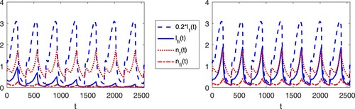
Figure 2. Trajectories in the $l_{fi}$–$n_{fi}$ phase plane with different parameter values of co-feeding efficiency, c. x-axis: $l_{fi}$, y-axis: $n_{fi}$. (a) c = 0, $R_{TBD}=0.47$, (b) c = 0.2, $R_{TBD}=0.7$, (c) c = 0.4, $R_{TBD}=1.08$, (d) c = 0.6, $R_{TBD}=1.71$, (e) c = 0.8, $R_{TBD}=2.86$.

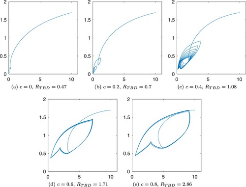
Table 1. Parameter values used in numerical simulations.

Parameters	Description	Value
$T\left(t\right)$	Temperature at time t	$19\cdot \sin \left(2\pi t/365\right)+12$
$b\left(t\right)$	Birth rate for ticks	$2000\cdot 0.5\cdot d_{pop}\left(t\right)$
H/D	Ratio of hosts for immature ticks	100
	to mature ticks
${\mu }_e$	mortality rate of eggs	0.02618
${\mu }_{ql}$, ${\mu }_{qn}$, ${\mu }_{qa}$	mortality rates of questing	0.0068, 0.0034, 0.00136
	larvae, nymphs, adults
${\mu }_{fl}\left(l_f\right)$	mortality rate of feeding larvae	$0.001428+0.01\cdot l_f$
${\mu }_{fn}\left(n_f\right)$	mortality rate of feeding nymphs	$0.000476+0.01\cdot n_f$
${\mu }_{fa}\left(a_f\right)$	mortality rate of feeding adults	$0.000408+0.1\cdot l_f$
${\text{β}}_{hl}$, ${\text{β}}_{hn}$, ${\text{β}}_{nh}$	transmission efficacy from hosts to larvae,	0.8, 0.8, 0.9
	hosts to nymphs, nymphs to hosts
c	probability of non-systemic infection	0.4
	when co-feeding with an infected nymph
γ	recovery rate of infected hosts	0.1
${\mu }_h$	mortality rate of hosts	0.0027
Parameters	Description, Dependence on temperature T (${}^{\circ }$C)
$d_e\left(t\right)$	development rate from eggs to larvae,
	$\left\{\begin{array}{ll}-0.0000112T(t{)}^2+0.002305T(t)-0.0185& \mathrm{i}\mathrm{f}T\left(t\right)\ge 8.4,\\ 0& \mathrm{o}\mathrm{t}\mathrm{h}\mathrm{e}\mathrm{r}\mathrm{w}\mathrm{i}\mathrm{s}\mathrm{e}.\end{array}\right.$
$d_l\left(t\right)$	development rate from larvae to nymphs,
	$\left\{\begin{array}{ll}0.0000303T(t{)}^2+0.000733T(t)-0.00706& \mathrm{i}\mathrm{f}T\left(t\right)\ge 7.4,\\ 0& \mathrm{o}\mathrm{t}\mathrm{h}\mathrm{e}\mathrm{r}\mathrm{w}\mathrm{i}\mathrm{s}\mathrm{e}.\end{array}\right.$
$d_n\left(t\right)$	development rate from nymphs to adults,
	$\left\{\begin{array}{ll}-0.00000796T(t{)}^2+0.00193T(t)-0.0161& \mathrm{i}\mathrm{f}T\left(t\right)\ge 8.7,\\ 0& \mathrm{o}\mathrm{t}\mathrm{h}\mathrm{e}\mathrm{r}\mathrm{w}\mathrm{i}\mathrm{s}\mathrm{e}.\end{array}\right.$
$d_{pop}\left(t\right)$	egg-laying rate of adult ticks,
	$\left\{\begin{array}{ll}-0.00001867T(t{)}^3+0.0008724T(t{)}^2-0.006195T\left(t\right)+0.01802& \mathrm{i}\mathrm{f}T\left(t\right)\ge 4,\\ 0& \mathrm{o}\mathrm{t}\mathrm{h}\mathrm{e}\mathrm{r}\mathrm{w}\mathrm{i}\mathrm{s}\mathrm{e}.\end{array}\right.$
${\alpha }_l\left(t\right)$	host-attaching rate for questing larvae, $0.0064\cdot H\left(T\right(t)-7)$
${\alpha }_n\left(t\right)$	host-attaching rate for questing nymphs, $0.0014\cdot H\left(T\right(t)-7)$
${\alpha }_a\left(t\right)$	host-attaching rates for questing adults, $24\cdot H\left(T\right(t)-7)$

It should be mentioned that unlike our formulation of co-feeding transmission, feeding ticks are not equally distributed in hosts [27]. Some modelling studies on co-feeding transmission used a negative binomial distribution to describe the pattern of tick aggregation and studied the effect on disease dynamics of tick distribution [31,39]. Also, we assumed that the mortality of feeding ticks only depends on the tick population of the same stages but not feeding ticks in other stages. Considering that ticks in different life stages can co-feed on a same host, the density-dependent mortality of feeding ticks in some life-stage may depend on the populations of feeding ticks in other stages as well as its own population. In this case monotonicity of tick population dynamics is not guaranteed and it remains a topics for future research to examine to global dynamics of the corresponding model system.

Disclosure statement

No potential conflict of interest was reported by the author(s).

References

- M. Daniel, M. Malý, V. Danielová, B. Kříž, and P. Nuttall, Abiotic predictors and annual seasonal dynamics of Ixodes ricinus, the major disease vector of Central Europe, Parasit. Vectors 8 (2015), p. 478.
- R.J. Eisen, L. Eisen, N.H. Ogden, and C.B. Beard, Linkages of weather and climate with Ixodes scapularis and Ixodes pacificus (Acari: Ixodidae), enzootic transmission of Borrelia burgdorferi, and Lyme disease in North America, J. Med. Entomol. 53(2) (2016), pp. 250–261.
- G. Fan, H.R. Thieme, and H. Zhu, Delay differential systems for tick population dynamics, J. Math. Biol. 71(5) (2015), pp. 1017–1048.
- G. Fan, Y. Lou, H.R. Thieme, and J. Wu, Stability and persistence in ODE models for populations with many stages, Math. Biosci. Eng. 12 (2015), pp. 661–686.
- H. Gaff, L. Gross, and E. Schaefer, Results from a mathematical model for human monocytic ehrlichiosis, Clin. Microbiol. Infect. 15(2) (2009), pp. 15–16.
- L. Gern and O. Rais, Efficient transmission of Borrelia burgdorferi between cofeeding Ixodes ricinus ticks (Acari: Ixodidae), J. Med. Entomol. 1(33) (1996), pp. 189–192.
- N.A. Hartemink, S.E. Randolph, S.A. Davis, and J.A.P. Heesterbeek, The basic reproduction number for complex disease systems: Defining R0 for tick-borne infections, Am. Nat. 171(6) (2008), pp. 743–754.
- J.M. Heffernan, Y. Lou, and J. Wu, Range expansion of Ixodes scapularis ticks and of Borrelia burgdorferi by migratory birds, Discrete Contin. Dyn. Syst. Ser. B 19(10) (2014), pp. 3147–3167.
- M.W. Hirsch, H.L. Smith, and X.Q. Zhao, Chain transitivity, attractivity, and strong repellors for semidynamical systems, J. Dyn. Differ. Equ. 13(1) (2001), pp. 107–131.
- R. Jennings, Y. Kuang, H.R. Thieme, J. Wu, and X. Wu, How ticks keep ticking in the adversity of host immune reactions, J. Math. Biol. 78(5) (2019), pp. 1331–1364.
- T. Kato, Perturbation Theory for Linear Operators, Springer Science & Business Media, Berlin Heidelberg, 2013.
- M. Kazimírová and I. Stibraniova, Tick salivary compounds: their role in modulation of host defences and pathogen transmission, Front. Cell. Infect. Microbiol. 3 (2013), p. 43.
- M. Labuda, L.D. Jones, T. Williams, V. Danielova, and P.A. Nuttall, Efficient transmission of tick-borne encephalitis virus between cofeeding ticks, J. Med. Entomol. 30(1) (1993), pp. 295–299.
- M. Labuda, O. Kozuch, E. Zuffová, E. Elecková, R.S. Hails, and P.A. Nuttall, Tick-borne encephalitis virus transmission between ticks cofeeding on specific immune natural rodent hosts, Virology 235(1) (1997), pp. 138–143.
- M.L. Levin, D. Fish, Density-dependent factors regulating feeding success of Ixodes scapularis larvae (Acari: Ixodidae), J. Parasitol. 84(1) (1988), pp. 36–43.
- Y. Lou, J. Wu, and X. Wu, Impact of biodiversity and seasonality on Lyme-pathogen transmission, Theor. Biol. Med. Model. 11(1) (2014), p. 50.
- Y. Lou, L. Liu, and D. Gao, Modeling co-infection of Ixodes tick-borne pathogens, Math. Biosci. Eng.14(5&6) (2017), pp. 1301–1316.
- M. Maliyoni, F. Chirove, H.D. Gaff, and K.S. Govinder, A stochastic tick-Borne disease model: Exploring the probability of pathogen persistence, Bull. Math. Biol. 79 (2017), 1999–2021.
- K. Nah, F.M.G. Magpantay, Å. Bede-Fazekas, G. Röst, A.J. Trájer, X. Wu, X. Zhang, and J. Wu, Assessing systemic and non-systemic transmission risk of tick-borne encephalitis virus in Hungary, PloS one 14(6) (2019), p. e0217206.
- R. Norman, R.G. Bowers, M. Begon, and P.J. Hudson, Persistence of tick-borne virus in the presence of multiple host species: tick reservoirs and parasite mediated competition, J. Theor. Biol. 200(1) (1999), pp. 111–118.
- R. Norman, D. Ross, M.K. Laurenson, and P.J. Hudson, The role of non-viraemic transmission on the persistence and dynamics of a tick borne virus–Louping ill in red grouse (Lagopus lagopus scoticus) and mountain hares (Lepus timidus), J. Math. Biol. 48(2) (2004), pp. 119–134.
- N.H. Ogden, M. Bigras-Poulin, C.J. O'callaghan, I.K. Barker, L.R. Lindsay, A. Maarouf, K.E.Smoyer-Tomic, D. Waltner-Toews, and D. Charron, A dynamic population model to investigate effects of climate on geographic range and seasonality of the tick Ixodes scapularis, Int. J. Parasitol. 35(4) (2005), pp. 375–389.
- P. Parola and D. Raoult, Ticks and tickborne bacterial diseases in humans: an emerging infectious threat, Clin. Infect. Dis. 32(6) (2001), pp. 897–928.
- J.H. Pettersson, I. Golovljova, S. Vene, and T.G. Jaenson, Prevalence of tick-borne encephalitis virus in Ixodes ricinus ticks in northern Europe with particular reference to Southern Sweden, Parasit. Vectors7(1) (2014), p. 102.
- S.E. Randolph, Abiotic and biotic determinants of the seasonal dynamics of the tick Rhipicephalus appendiculatus in South Africa, Med. Vet. Entomol. 11(1) (1997), pp. 25–37.
- S.E. Randolph, Transmission of tick-borne pathogens between co-feeding ticks: Milan Labuda's enduring paradigm, Ticks Tick-Borne Dis. 2(4) (2011), pp. 179–182.
- S.E. Randolph, L. Gern, and P.A. Nuttall, Co-feeding ticks: epidemiological significance for tick-borne pathogen transmission, Parasitol. Today 12(12) (1996), pp. 472–479.
- S.E. Randolph, D. Miklisova, J. Lysy, D.J. Rogers, and M. Labuda, Incidence from coincidence: patterns of tick infestations on rodents facilitate transmission of tick-borne encephalitis virus, Parasitol.118(2) (1999), pp. 177–186.
- D. Richter, R. Allgöwer, and F.R. Matuschka, Co-feeding transmission and its contribution to the perpetuation of the Lyme disease spirochete Borrelia afzelii, Emerg. Infect. Dis. 8(12) (2002), pp. 1421–1425.
- R. Rosà and A. Pugliese, Effects of tick population dynamics and host densities on the persistence of tick-borne infections, Math. Biosci., 208(1) (2007), pp. 216–240.
- R. Rosà, A. Pugliese, R. Norman, and P.J. Hudson, Thresholds for disease persistence in models for tick-borne infections including non-viraemic transmission, extended feeding and tick aggregation, J. Theor. Biol. 224(3) (2003), pp. 359–376.
- H.L. Smith, Monotone dynamical systems: an introduction to the theory of competitive and cooperative systems, Amer. Math. Soc. 41 (1995), pp. 81–84.
- P. Van den Driessche and J. Watmough, Reproduction numbers and sub-threshold endemic equilibria for compartmental models of disease transmission, Math. Biosci. 180(1–2) (2002), pp. 29–48.
- M.J. Voordouw, Co-feeding transmission in Lyme disease pathogens, Parasitology 142(2) (2015), pp. 290–302.
- W. Wang and X.Q. Zhao, Threshold dynamics for compartmental epidemic models in periodic environments, J. Dyn. Differ. Equ. 20(3) (2008), pp. 699–717.
- A. White, E. Schaefer, C.W. Thompson, C.M. Kribs, and H. Gaff, Dynamics of two pathogens in a single tick population, Lett. Biomath. 6(1) (2019), pp. 50–66.
- X. Wu and J. Wu, Diffusive systems with seasonality: eventually strongly order-preserving periodic processes and range expansion of tick populations, Canad. Appl. Math. Quart. 20 (2012), pp. 557–587.
- J. Wu, X. Zhang, Transmission Dynamics of Tick-Borne Diseases with Co-Feeding, Developmental and Behavioural Diapause, Springer Nature, Switzerland AG, 2020.
- X. Zhang and J. Wu, Implications of vector attachment and host grooming behaviour for vector population dynamics and distribution of vectors on their hosts, Appl. Math. Model. 81 (2020), pp. 1–15.
- X. Zhang, X. Wu, and J. Wu, Critical contact rate for vector-host-pathogen oscillation involving co-feeding and diapause, J. Biol. Syst. 25(04) (2017), pp. 657–675.
- X.Q. Zhao, Dynamical Systems in Population Biology, Springer, New York, 2003.