
 ?Mathematical formulae have been encoded as MathML and are displayed in this HTML version using MathJax in order to improve their display. Uncheck the box to turn MathJax off. This feature requires Javascript. Click on a formula to zoom.
Abstract
This paper studies a delayed viral infection model with diffusion and a general incidence rate. A discrete-time model was derived by applying nonstandard finite difference scheme. The positivity and boundedness of solutions are presented. We established the global stability of equilibria in terms of by applying Lyapunov method. The results showed that if
is less than 1, then the infection-free equilibrium
is globally asymptotically stable. If
is greater than 1, then the infection equilibrium
is globally asymptotically stable. Numerical experiments are carried out to illustrate the theoretical results.
1. Introduction
Mathematical models that describe within-host dynamics have been proposed and studied by constructing corresponding differential equations to get a better understanding of viral processes, particularly, their global dynamics behaviour has been investigated [Citation1, Citation2, Citation14, Citation17, Citation21, Citation28, Citation29, Citation32, Citation35–37]. For example, Wang and Zhou [Citation32] studied the following model:
(1)
(1) where T, I, C and V represent the concentrations of the uninfected cell, shorted-lived infected cells, chronically infected cells and free virus particles, respectively. s is the source term for uninfected cells. β represents the infection rate. ϵ is the efficacy of the therapy.
and c are the mortality rates of uninfected cells, short infected cells, chronically infected cells and virus, respectively. The fractions α and
are the probabilities that, upon infection, an uninfected cell will become either chronically infected or short-lived infected.
and
where
and
are the average numbers of virions produced in the lifetime of short-lived and chronically infected cells, respectively.
and
are the efficacy of the therapy.
and
are the intracellular delays. The global dynamics of the model have been studied by constructing Lyapunov functionals. For more details, one can refer to [Citation32]. The key assumption in model (Equation1
(1)
(1) ) is that cells and viruses are well mixed, and the mobility of viruses was ignored. So, in order to study the influences of spatial structures of virus dynamics, Wang et al. [Citation30] studied the following model:
(2)
(2) where
,
and
represent the densities of uninfected cells, infected cells and free virus at position x and at time t, respectively. τ is the intracellular delay. D is the diffusion coefficient and Δ is the Laplacian operator.
The bilinear incidence rate used in models (Equation1
(1)
(1) ) and (Equation2
(2)
(2) ) is a simple description of the infection. Though the incidence rates
,
and
are improved forms which are more commonly used [Citation22, Citation26, Citation31], the general incidence rates
,
and
can help us gain the unification theory by the omission of unessential details [Citation7, Citation8, Citation11, Citation13]. So, motivated by [Citation30, Citation32], we consider the following model with a general incidence rate which is similar to the one in [Citation7]
(3)
(3)
is the general incidence rate and satisfies the following hypotheses:
(4)
(4) It is easy to check that a class of functions
satisfying (Equation4
(4)
(4) ) includes some common used nonlinear incidence functions such as
,
and
for
.
The initial conditions of model (Equation3(3)
(3) ) are given as
(5)
(5) and we have considered model (Equation3
(3)
(3) ) with homogeneous Neumann boundary conditions
(6)
(6) where
, Ω is a bounded interval in
and
denotes the outward normal derivative on
.
As we know, it is difficult or even impossible to find the exact analytical solutions for most nonlinear models, such as (Equation3(3)
(3) ). In order to perform numerical simulations, we need to seek an efficient discrete method to discretize such nonlinear continuous models. However, some classical numerical discrete methods are unsuccessful in preserving the quantitative properties of corresponding continuous model. For example, for classical forward Euler's method, if the step size is selected small enough and the positivity conditions can be satisfied, then it can be shown that local asymptotic stability for an equilibrium is preserved while in some special cases numerical instability or Hopf bifurcation may appear. Thus how to design a feasible discrete scheme so that the same quantitative behaviours of solutions to the corresponding continuous models can be efficiently preserved is a challenging and interesting task. Recently, an interesting method which is called non-standard finite difference (NSFD) scheme has been proposed by Mickens [Citation18, Citation19]. NSFD has been applied to obtain discrete-time epidemic models [Citation4, Citation6, Citation9, Citation10, Citation20, Citation24, Citation25, Citation34] and references therein. Hence, motivated by the work of [Citation18, Citation19], we apply the NSFD scheme on model (Equation3
(3)
(3) ), then we obtain
(7)
(7) Set
be a bounded interval in
. Let
be the time step size and
be the space step size with N being a positive integer. Assume that there exist four integers
(i=1,2,3,4) with
. Denote the mesh grid point as
with
and
.
are the approximations of solution
at the discrete-time points. For simplicity, let
be the approximation solutions at the time
, where
and the notation
denotes the transposition of a vector. The initial conditions of model (Equation7
(7)
(7) ) are
(8)
(8) and the discrete boundary conditions are
The main purpose of this paper is to demonstrate the discretized model (Equation7
(7)
(7) ) derived by applying NSFD scheme can efficiently preserves the global dynamical properties to the original model (Equation3
(3)
(3) ). The rest of this paper is organized as follows. In Section 2, we study the dynamical behaviour of the continuous model (Equation3
(3)
(3) ). In Section 3, we investigate the global dynamics of discrete model (Equation7
(7)
(7) ). An example, along with numerical simulations is presented in Section 4 to validate the theoretical results. A brief conclusion ends the paper.
2. Dynamical analysis of model (3)
2.1. Preliminaries
Let be the space of continuous functions from the topological space
into the space
. Denote
be the Banach space of continuous functions from
into
with the usual supremum normal, and
. When convenient, we identify an element
as a function from
into
defined by
. We adopt the notation that for
, a function
induces functions
for
, defined by
for
. Let
. It follows from [Citation3] that the
-realization of
generates an analytic semi-group
on
.
Theorem 2.1
For any given initial data satisfying the condition (Equation5
(5)
(5) ), there exists a unique solution of problem (Equation3
(3)
(3) )–(Equation6
(6)
(6) ) defined on
and this solution remains non-negative and bounded for all
.
Proof.
For any we define
as follows. For any
,
We now reformulate (Equation3
(3)
(3) )–(Equation6
(6)
(6) ) as the abstract functional differential equation
(9)
(9) where
and
. It is clear that F is locally Lipschitz in
. It follows from [Citation5, Citation15, Citation16, Citation27, Citation33] that system (Equation9
(9)
(9) ) admits a unique local solution on
, where
is the maximal existence time for the solution of system (Equation9
(9)
(9) ).
In order to demonstrate the boundedness of solutions. Define and
, it then follows from model (Equation3
(3)
(3) ) that
Then we have
implying T, I and C are bounded.
From model (Equation3(3)
(3) )–(Equation6
(6)
(6) ), we deduce that V satisfies
(10)
(10) Let
be a solution to the ordinary differential equation
Then we get
,
. Thus
follows from the comparison principle [Citation23]. Therefore,
Based on the above analysis, we have demonstrated that
,
,
and
are bounded in
. It then follows from the standard theory for semilinear parabolic systems [Citation12] that
.
Let with
and
. For any
and any
, we obtain
Recall from (Equation4
(4)
(4) ) that
for all
. Therefore, for any
, we have
and
Thus we can demonstrate that for small enough ρ,
which implies that
We are now prepared to refer to key results from the literature. Denote
,
and
, it then follows from [Citation15] that (Equation3
(3)
(3) )–(Equation6
(6)
(6) ) has a unique mild solution
for
. Furthermore, since the semigroup
is analytic [Citation3]. Thus it follows from [Citation33] that the mild solution is classic for
. This completes the proof.
The dynamical outcomes of model (Equation3(3)
(3) ) will be determined by the basic reproduction number
, which is given by
It is clear that model (Equation3
(3)
(3) ) always has an infection-free equilibrium
and any positive equilibrium, denoted by
, must satisfy
(11)
(11) Simple calculation shows that
and
satisfies
It is easy to show that
According to (Equation4
(4)
(4) ), calculating shows
. Thus there exists a unique
such that
if and only if
. So, a unique infection equilibrium
exists when
.
Theorem 2.2
If , then the only equilibrium is the infection-free equilibrium
. If
, then there exists a unique infection equilibrium
.
2.2. Stabilities of equilibria
Theorem 2.3
If , then the infection-free equilibrium
of model (Equation3
(3)
(3) ) is globally asymptotically stable.
Proof.
Define a Lyapunov functional
For convenience, we let
and
( i = 1, 2, 3, 4) for any
. Calculating the time derivative of
along a solution of model (Equation3
(3)
(3) ), we obtain
Recall that
and (Equation4
(4)
(4) ), we obtain
Recall the condition (Equation4
(4)
(4) ), it is easy to show that
whenever
. Moreover, it can be shown that the largest invariant set
is the singleton
. By LaSalle's Invariance Principle, the infection-free equilibrium
of model (Equation3
(3)
(3) ) is globally asymptotically stable when
. This completes the proof.
Theorem 2.4
If , then the infection equilibrium
is globally asymptotically stable.
Proof.
Constructing a Lyapunov functional as follows:
where
for all x>0 and with a global minimum
. In the calculation that follows we will use the equilibrium equations
and note that
, and
. Then, calculating the time derivative of
along a solution of model (Equation3
(3)
(3) ), we obtain
Recall the conditions (Equation4
(4)
(4) ), we then obtain that
whenever
. Moreover, it can be shown that the largest invariant set
is the singleton
. By LaSalle's Invariance Principle, the infection equilibrium
of model (Equation3
(3)
(3) ) is globally asymptotically stable when
. This completes the proof.
3. Dynamical analysis of model (7)
3.1. Preliminary results
In this section, we dedicate to the investigation of the discrete model (Equation7(7)
(7) ). It is easy to see that the discrete model (Equation7
(7)
(7) ) has the same equilibria as model (Equation3
(3)
(3) ): the infection-free equilibrium
and the infection equilibrium
. In the following, we first show that the solution of model (Equation7
(7)
(7) ) is non-negative and bounded. To this end, rewriting the discrete model (Equation7
(7)
(7) ) yields
(12)
(12) where matrix A of dimension
is given by
with
,
and
. It is easy to show that A is a strictly diagonally dominant matrix. Hence, A is non-singular. We then obtain that
Theorem 3.1
For any and
, the solutions of the discrete model (Equation7
(7)
(7) ) remain nonnegative and bounded for all
.
Proof.
We can claim that for all
. In fact, assuming the contrary and letting
be the first time such that
and
,
,
,
for all
. Since,
Note that the conditions of (Equation4
(4)
(4) ), we then obtain
, which contradicts our assumption and so
for all
. Moreover, it is easy to prove that the sequences
,
and
are non-negative by using mathematical induction.
Next, we establish the boundedness of solutions. To this end, we define a sequence as follows:
Then, we have
where
. Thus we obtain
By using induction, we easily obtain
Thus
which implies that
is bounded. Therefore,
,
and
are bounded.
By the last equation of model (Equation7(7)
(7) ) that
Note that
and
are bounded, there exists two positive constant
such that
,
for
. Thus we have
By induction, we have
implying
is bounded. This completes the proof.
3.2. Global stability
Theorem 3.2
For any ,
, if
, then the infection-free equilibrium
of system (Equation7
(7)
(7) ) is globally asymptotically stable.
Proof.
Consider the following discrete Lyapunov functional:
Then we have
The last inequality is followed by the condition (Equation4
(4)
(4) ). Thus if
, then we have
for all
, which implies that
is a monotone decreasing sequence. Since
, there is a limit
which implies that
, from which we get
and
. We discuss two cases: (i) if
, from model (Equation7
(7)
(7) ), we obtain
,
, for all
; (ii) if
, by
and from model (Equation7
(7)
(7) ), we have
,
,
. Thus concluding the above discussion implies that
is globally asymptotically stable. This completes the proof.
Theorem 3.3
For any and
, if
, then the infection equilibrium
of model (Equation3
(3)
(3) ) is globally asymptotically stable.
Proof.
Define
where
for all x>0. Obviously,
has a global minimum at x = 1 and
.
Recall that model (Equation12(12)
(12) ) and the infection equilibrium conditions (Equation11
(11)
(11) ), we then have the difference of
satisfies
It follows from the condition (Equation4
(4)
(4) ) that
. Recall that
for all x>0, we then obtain
, for all
. This implies that
is monotone decreasing sequence. Since
, there is a limit
. Hence,
. Furthermore, from model (Equation7
(7)
(7) ), it can be shown that
,
,
,
, for all
, which implies that
of model (Equation7
(7)
(7) ) is globally asymptotically stable. This completes the proof.
4. Numerical simulations
In this section, we perform numerical simulation to validate the main theoretical results obtained in previous sections. To this end, we reduce model (Equation3(3)
(3) ) to the one with
, then the model reads as
(13)
(13) with the homogeneous Neumann boundary conditions
and initial conditions
The corresponding discrete model to (Equation13
(13)
(13) ) is given by
(14)
(14) with the discrete boundary condition
and the discrete initial conditions
Let
, D = 0.05,
and
. For convenience, we set a = 0.00001,
,
,
and
in the following simulations. Some of the parameter values for these simulations are selected from [Citation32]. The numerical implementation of (Equation13
(13)
(13) ) is carried out using the NSFD scheme described in (Equation14
(14)
(14) ). We first select the parameter values: s = 1000,
, d = 0.01,
,
, a = 0.5,
,
,
,
, c = 13. By a simple calculation, we have
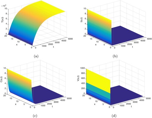
. Hence, in this case, the infection-free equilibrium
is globally asymptotically stable, which means that the virus is cleared and the infection dies out. Figure validates the above analysis.
Figure 1. , the infection-free equilibrium
is globally asymptotically stable.
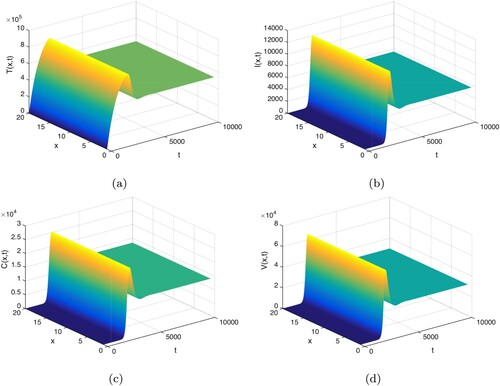
Next, we select and keep the other parameters are the same with Figure . In this case, we have
and the unique infection equilibrium
is globally asymptotically stable, which means that the virus persists in the host and the infection becomes chronic. Figure confirms this observation.
Figure 2. , the infection equilibrium
is globally asymptotically stable.
5. Conclusion
In this paper, we have formulated a delayed and diffusive viral infection model incorporating shorted-lived and chronically infected cells and general nonlinear incidence function. Then, by applying NSFD scheme, we presented an efficient numerical method for the corresponding continuous model. Theoretically, we have shown that the stability conditions for the equilibria are identical in case of both the continuous and discrete models. Specifically, if , then the infection-free equilibrium
is globally asymptotically stable; if
, then the infection equilibrium
is globally asymptotically stable. The results show that the NSFD scheme has the advantage that the positivity, boundedness and global properties of solutions for original continuous model are efficiently preserved.
As far as we know, there are few delayed and diffusive virus models considering both the shorted-lived and chronically infected cells, and no theoretical analysis has been made on this kind of models. Here, our main contribution is to construct suitable Lyapunov functional for both the continuous-time and discrete-time virus models, and present a general method to analyse this kind of models. Based on the above obtained results, one can extend this method to more complicated models.
Disclosure statement
No potential conflict of interest was reported by the author(s).
Additional information
Funding
References
- Z. Bai and Y. Zhou, Dynamics of a viral infection model with delayed CTL response and immune circadian rhythm, Chaos Solitons Fract. 45(9–10) (2012), pp. 1133–1139.
- L. Cai and X. Li, Stability and Hopf bifurcation in a delayed model for HIV infection of CD4 +T cells, Chaos Solitons Fract. 42(1) (2009), pp. 1–11.
- D. Daners and P.K. Medina, Pitman Research Notes in Math. Ser., Vol. 279, Abstract Evolution Equations, Periodic Problems and Applications, 1992.
- D. Ding, W. Qin, and X. Ding, Lyapunov functions and global stability for a discretized multigroup SIR epidemic model, Discrete Contin. Dyn. Syst. B 20 (2015), pp. 1971–1981.
- W.E. Fitzgibbon, Semilinear functional differential equations in Banach space, J. Differ. Equ. 29 (1978), pp. 1–14.
- Y. Geng, J. Xu, and J. Hou, Discretization and dynamic consistency of a delayed and diffusive viral infection model, Appl. Math. Comput. 316 (2018), pp. 282–295.
- K. Hattaf, A.A. Lashari, Y. Louartassi, and N. Yousfi, A delayed SIR epidemic model with general incidence rate, Electron. J. Qual. Theor. 3 (2013), pp. 1–9.
- K. Hattaf and N. Yousfi, Global properties of a discrete viral infection model with general incidence rate, Math. Methods Appl. Sci. 39(5) pp. 998–1004.
- K. Hattaf and N. Yousfi, Global properties of a discrete viral infection model with general incidence rate, Math. Methods Appl. Sci. 39 (2016), pp. 998–1004.
- K. Hattaf and N. Yousfi, A numerical method for delayed partial differential equations describing infectious diseases, Comput. Math. Appl. 72 (2016), pp. 2741–2750.
- K. Hattaf, N. Yousfi, and A. Tridane, Mathematical analysis of a virus dynamics model with general incidence rate and cure rate, Nonlinear Anal. Real World Appl. 13 (2012), pp. 1866–1872.
- D. Henry, Gerometric Theory of Semilinear Parabolic Equations, Lecture Notes in Mathematics, Vol. 840, Springer-Verlag, Berlin, New York, 1993.
- G. Huang, Y. Takeuchi, and W.B. Ma, Lyapunov functionals for delay differential equations model of viral infections, SIAM J. Appl. Math. 70 (2010), pp. 2693–2708.
- M.Y. Li and H. Shu, Impact of intracellular delays and target-cell dynamics on in vivo viral infections, SIAM J. Appl. Math. 70 (2010), pp. 2434–2448.
- R.H. Martin and H.L. Smith, Abstract functional differential equations and reaction-diffusion systems, Trans. Amer. Math. Soc. 321 (1990), pp. 1–44.
- R.H. Martin and H.L. Smith, Reaction-diffusion systems with time delays: monotonicity, invariance, comparison and convergence, J. Reine. Angew. Math. 413 (1991), pp. 1–35.
- C.C. McCluskey and Y. Yang, Global stability of a diffusive virus dynamics model with general incidence function and time delay, Nonlinear Anal. Real World Appl. 25 (2015), pp. 64–78.
- R.E. Mickens, Nonstandard Finite Difference Models of Differential Equations, World Scientific, Singapore, 1994.
- R.E. Mickens, Dynamics consistency: a fundamental principle for constructing nonstandard finite difference scheme for differential equation, J. Diff. Equ. Appl. 9 (2003), pp. 1037–1051.
- Y. Muroya, Y. Bellen, Y. Enatsu, and Y. Nakata, Global stability for a discrete epidemic model for disease with immunity and latency spreading in a heterogeneous host population, Nonlinear Anal. Real World Appl. 13 (2013), pp. 258–274.
- Y. Nakata, Global dynamics of a cell mediated immunity in viral infection models with distributed delays, J. Math. Anal. Appl. 375 (2011), pp. 14–27.
- M.A. Obaid and A.M. Elaiw, Stability of virus infection models with antibodies and chronically infected cells, Abstract Appl. Anal. 2014 (2014), pp.1–12. Article ID 650371
- M.H. Protter and H.F. Weinberger, Maximum Principles in Differential Equations, Prentice Hall, Englewood Cliffs, 1967.
- W. Qin, L. Wang, and X. Ding, A non-standard finite difference method for a hepatitis B virus infection model with spatial diffusion, J. Differ. Equ. Appl. 20 (2014), pp. 1641–1651.
- P. Shi and L. Dong, Dynamical behaviors of a discrete HIV-1 virus model with bilinear infective rate, Math. Methods Appl. Sci. 37 (2014), pp. 2271–2280.
- X.Y. Song and U. Neumann Avidan, Global stability and periodic solution of the viral dynamics, J. Math. Anal. Appl. 329 (2007), pp. 281–297.
- C.C. Travis and G.F. Webb, Existence and stability for partial functional differential equations, Trans. Amer. Math. Soc. 200 (1974), pp. 395–418.
- T. Wang, Z. Hu, F. Liao, and W. Ma, Global stability analysis for delayed virus infection model with general incidence rate and humoral immunity, Math. Comput. Simul. 89 (2013), pp. 13–22.
- F. Wang, Y. Huang, and X. Zou, Global dynamics of a PDE in-host viral model, Appl. Anal. 93 (2014), pp. 2312–2329.
- K. Wang, W. Wang, and S. Song, Dynamics of an HBV model with diffusion and delay, J. Theor. Biol. 253(1) (2008), pp. 36–44.
- Z.P. Wang and R. Xu, Stability and Hopf bifurcation in a viral infection model with nonlinear incidence rate and delayed immune response, Commun. Nonlinear. Sci. 17 (2012), pp. 964–978.
- S. Wang and Y. Zhou, Global dynamics of an in-host HIV-1 infection model with the long-lived infected cells and four intracellular delays, Int. J. Biomath. 5 (06)(2012), pp. 1250058.
- J. Wu, Theory and Applications of Partial Functional Differential Equations, Springer, New York, 1996.
- J. Xu, Y. Geng, and J Hou, A non-standard finite difference scheme for a delayed and diffusive viral infection model with general nonlinear incidence rate, Comput. Math. Appl. 74(8) (2017), pp. 1782–1798.
- J. Xu and Y. Zhou, Bifurcation analysis of HIV-1 infection model with cell-to-cell transmission and immune response delay, Math. Biosci. Eng. 13 (2016), pp. 343–367.
- J. Xu, Y. Zhou, Y. Li, and Y. Yang, Global dynamics of a intracellular infection model with delays and humoral immunity, Math. Methods. Appl. Sci. 39 (2016), pp. 5427–5435.
- Y. Yang, J. Zhou, X. Ma, and T. Zhang, Nonstandard finite difference scheme for a diffusive within-host virus dynamics model with both virus-to-cell and cell-to-cell transmissions, Comput. Math. Appl. 72 (2016), pp. 1013–1020.