Dynamic mechanism of multiple bursting patterns in a whole-cell multiscale model with calcium oscillations

Abstract

The dynamic mechanism of a whole-cell model containing electrical signalling and two-compartment Ca${}^{2+}$ signalling in gonadotrophs is investigated. The transition from spiking to bursting by Hopf bifurcation of the fast subsystem about the slow variable is detected via the suitable parameters. When the timescale of K${}^{+}$ gating variable is changed, the relaxation oscillation with locally small fluctuation, chaotic bursting and mixed-mode bursting (MMB) are revealed through chaos. In addition, the bifurcation of $[{\mathrm{C}\mathrm{a}}^{2+}{]}_i$ with regard to $\left[\mathrm{I}{\mathrm{P}}_3\right]$ is analysed, showing periodic solutions, torus, period doubling solutions and chaos. Finally, hyperpolarizations and torus canard-like behaviours of the full system under a set of specific parameters are elucidated.

Keywords:

• Chaotic bursting
• mixed-mode bursting
• torus canard-like
• hyperpolarization
• bifurcation
• torus

1. Introduction

Calcium signal is essential in cells, participating in and controlling many important cellular biological processes and mechanisms, such as the contraction of muscle cells, the release of neurotransmitters from neurons and astrocytes, and the activation of eggs, the healing and metabolism of liver and pancreatic trauma [1–3], as well as cell maturation, differentiation and death [4–6]. Since the Ca${}^{2+}$ oscillation was first observed, the discussion of its molecular mechanism from the aspects of experiment and model has never stopped [7–9].

Intracellular interactions between a variety of elements regulate Ca${}^{2+}$ signals: for example, the entry and discharge through plasma membrane (PM), the release and re-extraction from intracellular stores, and the buffering of endogenous Ca${}^{2+}$ buffers. In detail, the link of hormones or other signalling molecules (glutamate, ATP, etc.) and the G protein-coupled receptor (GPCRs) on PM activates intracellular phospholipase C (PLC), hydrolyses phospholipid, especially phosphatidylinositol-4, 5-diphosphate (PIP2), located in the inner layer of PM. Hydrolysis of PIP2 produces two products: diacylglycerol (DAG) and inositol 1, 4, 5-triphosphate (IP${}_3$). IP${}_3$ and Ca${}^{2+}$ are combined to IP${}_3$ receptor (IP${}_3$R ), and IP${}_3$R in turn regulates the release of Ca${}^{2+}$ from endoplasmic reticulum (ER). A Ca${}^{2+}$ leakage (leak), from ER to the cytoplasm, may exist. At the same time, Ca${}^{2+}$ in the cytoplasm can be pumped into ER through the Ca${}^{2+}$ -ATP enzyme (SERCA) on the sarcoplasmic reticulum. Extracellular Ca${}^{2+}$ ions enter the cells through the source-operated Ca${}^{2+}$ entrance, and intracellular Ca${}^{2+}$ is discharged into the extracellular matrix through the PM ATP enzyme (PMCA). 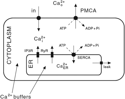Parts of the principle of intracellular Ca${}^{2+}$ signal transduction pathway are shown in Figure 1 [10].

Figure 1. The physiological mechanism of the flux balance of Ca${}^{2+}$.

Based on the biological principles of Ca${}^{2+}$ signals, the concept of Ca${}^{2+}$ ‘toolbox’ [11] can be used to understand Ca${}^{2+}$ oscillation in various cells. The common opinion is that the combination of IP${}_3$ and Ca${}^{2+}$ opening IP${}_3$R channels is the most important toolbox component, which is modulated to get kinds of Ca${}^{2+}$ signals with distinguished frequencies and patterns, presented as various nonlinear terms in the mathematical models [12–14]. As a result, the dynamic system theory is a powerful tool to discuss the behaviour of Ca${}^{2+}$ signals, especially the bifurcation theory can give the mechanism of different Ca${}^{2+}$ signal patterns [12,15,16]. Meanwhile, the change of intracellular Ca${}^{2+}$ inevitably causes the difference of membrane potential, forming a variety of spiking modes of neurons, in turn, the change of membrane potential also causes distinguished Ca${}^{2+}$ oscillation patterns. The motivation gives multiple mathematical models [17,18] describing the interaction between the membrane potential and Ca${}^{2+}$ oscillations. Because of the multiple timescales in the two parts, such models generally correspond to the slow–fast systems, with which the bifurcation analysis shows the mechanism to generate complex spiking patterns and Ca${}^{2+}$ oscillations. As typical examples, [19] has shown a complete topological classification of bursting about codimension-1 bifurcation, including 120 different topological types. Additionally, it is obtained that the neuron has multiple kinds of bursting: ‘fold/fold’, ‘Hopf/Hopf’, ‘Hopf/homoclinic’ and ‘fold cycle/homoclinic’ burstings by bifurcation analysis [18,20,21].

Li et al. [10,22] proposed a whole model including PM and ER parts in gonadotrophs in order to show the bursting caused by Ca${}^{2+}$ oscillations on the basis of the experimental description. The outstanding feature of the model is to consider Ca${}^{2+}$ signals in both the cytosol and ER, which together with the membrane potential give a system with a fast and two slow time scales, and the slow scales according to Ca${}^{2+}$ are not at the same time level. Such model extremely tends to declare chaotic bursting, discussed in the similar system in [17]. Our purpose is to investigate the model with two compartments containing only K${}^{+}$, Ca${}^{2+}$ and calcium dependent potassium currents in order to find the interesting spiking, bursting, mixed-mode bursting (MMB), chaotic bursting, behaviour like torus canard [23,24] and so on combined with bifurcation theory.

The paper is organized as follows. Section 2 introduces the form of the model to be investigated. In Section 3, the spiking patterns according to $[{\mathrm{C}\mathrm{a}}^{2+}{]}_i$ and time scale are explored. In Section 4, the spiking transition and MMB depending on the time scale are discussed. The dynamics of $[{\mathrm{C}\mathrm{a}}^{2+}{]}_i$ is studied in Section 5, which shows periodic solutions, torus and chaos. In Sections 6–7, hyperpolarizations related to $[{\mathrm{C}\mathrm{a}}^{2+}{]}_i$ and torus canard-like pattern are declared. The last part is the conclusion in Section 8.

2. System model

The paper is devoted to a whole-cell model containing electrical signalling and two-compartment Ca${}^{2+}$ signalling in gonadotrophs of the form: (1) $\begin{array}{rl}& C_m\frac{\mathrm{d}V}{\mathrm{d}t}=-I_{\mathrm{C}\mathrm{a}}-I_{\mathrm{K}}-I_{\mathrm{K}\mathrm{C}\mathrm{a}},\\ & \frac{\mathrm{d}\omega }{\mathrm{d}t}=\varphi \left({\omega }_{\mathrm{\infty }}\right(V)-\omega )/{\tau }_{\omega }\left(V\right),\end{array}$(1) where $\begin{array}{rl}& I_{\mathrm{C}\mathrm{a}}=g_{\mathrm{C}\mathrm{a}}{m}_{\mathrm{\infty }}\left(V\right)(V-V_{\mathrm{C}\mathrm{a}}),\\ & I_{\mathrm{K}}=g_K\omega (V-V_{\mathrm{K}}),\\ & I_{\mathrm{K}\mathrm{C}\mathrm{a}}=g_{\mathrm{K}\mathrm{C}\mathrm{a}}\frac{[C{a}^{2+}{]}_i^4}{[C{a}^{2+}{]}_i^4+K_{\mathrm{K}\mathrm{C}\mathrm{a}}^4}(V-V_{\mathrm{K}}),\end{array}$with $\begin{array}{rl}& m_{\mathrm{\infty }}\left(V\right)=0.5[1+\tanh ((V-v_1)/v_2\left)\right],\\ & {\omega }_{\mathrm{\infty }}\left(V\right)=0.5[1+\tanh ((V-v_3)/v_4\left)\right],\\ & {\tau }_{\omega }\left(V\right)=1/\cosh \left(\right(V-v_3\left)/\right(2v_4\left)\right).\end{array}$V is the membrane potential, ω is the gating variable for the voltage-gated potassium. The functions $I_{\mathrm{C}\mathrm{a}}$, $I_K$ and $I_{\mathrm{K}\mathrm{C}\mathrm{a}}$ represent Ca${}^{2+}$ current, K${}^{+}$ current and Ca${}^{2+}$ dependent K${}^{+}$ current, respectively.

The flux balance equations (see Figure 1) for ER and PM are shown as follows: (2) $\begin{array}{rl}& \frac{\mathrm{d}[{\mathrm{C}\mathrm{a}}^{2+}{]}_i}{\mathrm{d}t}=\frac{f_i}{v_i}[J_{\mathrm{E}\mathrm{R}}^{\mathrm{o}\mathrm{u}\mathrm{t}}-J_{\mathrm{E}\mathrm{R}}^{\mathrm{i}\mathrm{n}}+ϵ(J_{\mathrm{P}\mathrm{M}}^{\mathrm{i}\mathrm{n}}-J_{\mathrm{P}\mathrm{M}}^{\mathrm{o}\mathrm{u}\mathrm{t}}\left)\right],\\ & \frac{\mathrm{d}h}{\mathrm{d}t}=A[K_d-([{\mathrm{C}\mathrm{a}}^{2+}{]}_i+K_d)h],\\ & \frac{\mathrm{d}[{\mathrm{C}\mathrm{a}}^{2+}{]}_T}{\mathrm{d}t}=\frac{f_iϵ}{v_i}[J_{\mathrm{P}\mathrm{M}}^{\mathrm{i}\mathrm{n}}-J_{\mathrm{P}\mathrm{M}}^{\mathrm{o}\mathrm{u}\mathrm{t}}],\end{array}$(2) where $\begin{array}{rl}& J_{\mathrm{P}\mathrm{M}}^{\mathrm{i}\mathrm{n}}=-\alpha I_{\mathrm{C}\mathrm{a}},\\ & J_{\mathrm{P}\mathrm{M}}^{\mathrm{o}\mathrm{u}\mathrm{t}}=J_{\mathrm{P}\mathrm{M}\mathrm{C}\mathrm{A}}=\frac{V_{\mathrm{P}\mathrm{M}\mathrm{C}\mathrm{A}}[{\mathrm{C}\mathrm{a}}^{2+}{]}_i^2}{K_{\mathrm{P}\mathrm{M}\mathrm{C}\mathrm{A}}^2+[{\mathrm{C}\mathrm{a}}^{2+}{]}_i^2},\\ & J_{\mathrm{E}\mathrm{R}}^{\mathrm{i}\mathrm{n}}=J_{\mathrm{S}\mathrm{E}\mathrm{R}\mathrm{C}\mathrm{A}}=\frac{V_{\mathrm{S}\mathrm{E}\mathrm{R}\mathrm{C}\mathrm{A}}[{\mathrm{C}\mathrm{a}}^{2+}{]}_i^2}{K_{\mathrm{S}\mathrm{E}\mathrm{R}\mathrm{C}\mathrm{A}}^2+[{\mathrm{C}\mathrm{a}}^{2+}{]}_i^2},\\ & J_{\mathrm{E}\mathrm{R}}^{\mathrm{o}\mathrm{u}\mathrm{t}}=J_{\mathrm{L}\mathrm{E}\mathrm{A}\mathrm{K}}+J_{\mathrm{R}\mathrm{y}\mathrm{R}}=\left[L+P_{\mathrm{I}\mathrm{P}3\mathrm{R}}{\left(\frac{\left[{\mathrm{C}\mathrm{a}}^{2+}{]}_{i}h\right[{\mathrm{I}\mathrm{P}}_3]}{\left(\right[I{P}_3]+K_i)\left(\right[{\mathrm{C}\mathrm{a}}^{2+}{]}_i+K_a)}\right)}^3\right]\\ & \left(\right[{\mathrm{C}\mathrm{a}}^{2+}{]}_{\mathrm{E}\mathrm{R}}-\left[{\mathrm{C}\mathrm{a}}^{2+}{]}_i\right),\\ & [{\mathrm{C}\mathrm{a}}^{2+}{]}_{\mathrm{E}\mathrm{R}}=\frac{[{\mathrm{C}\mathrm{a}}^{2+}{]}_T-[{\mathrm{C}\mathrm{a}}^{2+}{]}_i}{\sigma }.\end{array}$$[{\mathrm{C}\mathrm{a}}^{2+}{]}_i$ is the free cytosolic Ca${}^{2+}$ between PM and ER. $[{\mathrm{C}\mathrm{a}}^{2+}{]}_T$ is the ‘total free Ca${}^{2+}$ ’ of the cell. $J_{\mathrm{P}\mathrm{M}\mathrm{C}\mathrm{A}}$ and $J_{\mathrm{S}\mathrm{E}\mathrm{R}\mathrm{C}\mathrm{A}}$ are pump fluxes, $J_{\mathrm{L}\mathrm{E}\mathrm{A}\mathrm{K}}$ is the unregulated leak conductance, and $J_{\mathrm{R}\mathrm{y}\mathrm{R}}$ is the RyR channel flux. h is the fraction of channels not inactivated by Ca${}^{2+}$.

Compared with the model in [22], the system (1(1) $\begin{array}{rl}& C_m\frac{\mathrm{d}V}{\mathrm{d}t}=-I_{\mathrm{C}\mathrm{a}}-I_{\mathrm{K}}-I_{\mathrm{K}\mathrm{C}\mathrm{a}},\\ & \frac{\mathrm{d}\omega }{\mathrm{d}t}=\varphi \left({\omega }_{\mathrm{\infty }}\right(V)-\omega )/{\tau }_{\omega }\left(V\right),\end{array}$(1) )–(2(2) $\begin{array}{rl}& \frac{\mathrm{d}[{\mathrm{C}\mathrm{a}}^{2+}{]}_i}{\mathrm{d}t}=\frac{f_i}{v_i}[J_{\mathrm{E}\mathrm{R}}^{\mathrm{o}\mathrm{u}\mathrm{t}}-J_{\mathrm{E}\mathrm{R}}^{\mathrm{i}\mathrm{n}}+ϵ(J_{\mathrm{P}\mathrm{M}}^{\mathrm{i}\mathrm{n}}-J_{\mathrm{P}\mathrm{M}}^{\mathrm{o}\mathrm{u}\mathrm{t}}\left)\right],\\ & \frac{\mathrm{d}h}{\mathrm{d}t}=A[K_d-([{\mathrm{C}\mathrm{a}}^{2+}{]}_i+K_d)h],\\ & \frac{\mathrm{d}[{\mathrm{C}\mathrm{a}}^{2+}{]}_T}{\mathrm{d}t}=\frac{f_iϵ}{v_i}[J_{\mathrm{P}\mathrm{M}}^{\mathrm{i}\mathrm{n}}-J_{\mathrm{P}\mathrm{M}}^{\mathrm{o}\mathrm{u}\mathrm{t}}],\end{array}$(2) ) ignores the external and leakage currents, and only considers the influence of $K^{+}$ and Ca${}^{2+}$ ions on the membrane potential. Without the evolution according to the space and emphasizing the different time scales, such a multi-scale model will produce complex dynamics. From a biological point of view, carrying signals in the form of Ca${}^{2+}$ oscillations can not only achieve intracellular signal transmission but also avoid the harm of high concentrations of Ca${}^{2+}$ to cells. Therefore, intracellular Ca${}^{2+}$ oscillations and the interaction mechanism with membrane potential is an invaluable subject.

3. Membrane potential oscillations related to Ca${}^{2+}$

3.1. Transition from spiking to bursting

We begin with the relationship between V and $[{\mathrm{C}\mathrm{a}}^{2+}{]}_i$. Figure 2 shows PM and ER oscillations where $\left[{\mathrm{I}\mathrm{P}}_3\right]=0.9\mu M,\varphi =12/s$ and other parameters can be found in Table A1. Figure 2(a) gives the oscillations of V and $[{\mathrm{C}\mathrm{a}}^{2+}{]}_i$. The red curve represents the time series of intracellular calcium concentration $[{\mathrm{C}\mathrm{a}}^{2+}{]}_i$ and the black curve indicates the trend of membrane potential V. While the concentration of free cytosolic Ca${}^{2+}$ between PM and ER oscillates, the membrane potential spikes and then bursts. For a clear description, we give a truncation from t = 0 to 20 in Figure 2(b) that combines the periodic spiking of V and the oscillation of $[{\mathrm{C}\mathrm{a}}^{2+}{]}_i$. During each of the up and down oscillations of $[{\mathrm{C}\mathrm{a}}^{2+}{]}_i$, the highest concentration leads to the wave valley of V corresponding to the hyperpolarization of the cell, however, the lowest one causes the spiking. On the other hand, the periodic change of action potential V affects the Ca${}^{2+}$ channel on the cell membrane, which is a remarkable reason for the $[{\mathrm{C}\mathrm{a}}^{2+}{]}_i$ oscillation.

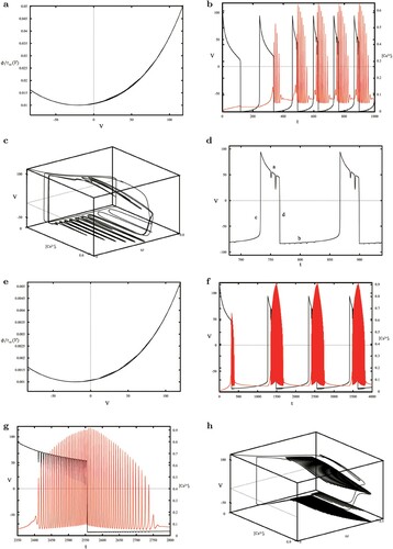
Figure 2. (a) The time series of V (the black curve) and $[{\mathrm{C}\mathrm{a}}^{2+}{]}_i$ (the red curve); (b–c) Enlargements of (a): a periodic spiking and a bursting of V; (d) the timescale curve of ω with the membrane potential V; (e) the combination of phase plot (the green curve) and bifurcation diagram on V-$[{\mathrm{C}\mathrm{a}}^{2+}{]}_i$ plane, where the equilibrium and limit cycle of the fast subsystem are shown in (f): the green and red curves indicate $V\mathrm{\&}\omega$ nullclines, intersecting at the equilibrium P surrounded by a stable limit cycle (the blue circle).

Figure 2(c) also explains the inhibitory effect of high concentration Ca${}^{2+}$ on V and the promoting effect of low concentration Ca${}^{2+}$. In other words, now calcium moves periodically after irregular oscillation. When $[{\mathrm{C}\mathrm{a}}^{2+}{]}_i$ rises upward, V falls back to the resting state, instead, the decreasing of $[{\mathrm{C}\mathrm{a}}^{2+}{]}_i$ gives the phenomenon of repetitive spiking. The results are consistent with the physiological mechanism.

The timescale curve of ω about the membrane potential V in Figure 2(d) tells us that ω is not a slow variable. Thus neglecting other system slow variables, Figure 2(e) is the projection of V and $[{\mathrm{C}\mathrm{a}}^{2+}{]}_i$ phase plot (the green curves) on the bifurcation diagram, indicating the rapid and repetitive spiking of the PM oscillator during the low concentration oscillation of Ca${}^{2+}$. HB represents the supercritical Hopf bifurcation point, corresponding to $[{\mathrm{C}\mathrm{a}}^{2+}{]}_i=0.3139$. With the increase of $[{\mathrm{C}\mathrm{a}}^{2+}{]}_i$, the equilibrium of the fast subsystem changes from the initial unstable node (the red curve) through the HB point to the stable (the black curve) and a stable limit cycle (SLC) appears on the left side of HB, forming a limit cycle of the whole system, as shown in Figure 2f, whose maximum and minimum amplitudes are denoted by the blue curve.

3.2. Relaxation oscillations caused by timescale changes

Next, we reduce the value of ϕ to 0.01 with the same other parameters in Figure 2. As a result, we get a system with one of fast variables changed into a slow one, as shown in Figure 3 (a). Figure 3(b) shows that when $[{\mathrm{C}\mathrm{a}}^{2+}{]}_i$ increases slowly, the PM goes through depolarization, overshoot and the membrane potential V decreases slightly. With the sudden increase of $[{\mathrm{C}\mathrm{a}}^{2+}{]}_i$, V begins to oscillate and continues to fall down, until $[{\mathrm{C}\mathrm{a}}^{2+}{]}_i$ reaches the maximum. After that, PM completes the repolarization and the hyperpolarization instantaneously. Finally, the oscillation decrease of $[{\mathrm{C}\mathrm{a}}^{2+}{]}_i$ pushes V into a slight hyperpolarization vibration. Therefore, a relaxation oscillation according to the shape of ‘a weak tip’ of $[{\mathrm{C}\mathrm{a}}^{2+}{]}_i$ becomes visible. The simulation in 3-d space (Figure 3c) shows that V has two parts of oscillation above and below the plane V = 0 with respect to $[{\mathrm{C}\mathrm{a}}^{2+}{]}_i$, corresponding to parts a and b in Figure 3d, while the two mutations across V = 0 correspond to c and d, respectively. When the time scale (Figure 3e) is reduced by 1/10, the relaxation oscillation phenomenon also appears, but ‘the strong tip shape’ of $[{\mathrm{C}\mathrm{a}}^{2+}{]}_i$, as shown in Figure 3f, makes the local oscillation of V stronger, enlarged in Figure 3 (g), and the concentrated oscillation of the two parts in the 3-d space is more obvious (Figure 3h). Choosing the plane $\omega =0.4$ as the Poincar$\acute{e}$ section, it can be seen from Figure 3(i) that the points on the section are stacked into two parts, where the small figure in the middle is the magnification of the upper part. There is a reason to consider that chaos occurs. In order to verify this conclusion, we calculate the maximum Lyapunov exponent of the system to find that its value is 4.28534.

Figure 3. (a) and (e) The timescale curves of ω about V indicate that ω is a slow variable at present at $\varphi =0.01$ and 0.001; (b) and (f) The relaxation vibrations with weak or strong local oscillations because of slow or fast frequency of $[{\mathrm{C}\mathrm{a}}^{2+}{]}_i$, where the red and black curves show the time series of $[{\mathrm{C}\mathrm{a}}^{2+}{]}_i$ and V, respectively; (c) and (h) The 3-d phase spaces consist of V, ω together with $[{\mathrm{C}\mathrm{a}}^{2+}{]}_i$ with $\varphi =0.01$ and 0.001, equipped by the partial enlargements (d) and (g); (i) Poincar$\acute{e}$ section $\omega =0.4$.

4. Chaotic and mixed-mode burstings according to ϕ

This section focuses on different forms of cell spiking as a result of variable ϕ. Figure 4 gives several solutions with regard to the membrane potential V. Using the parameters in Table A1 with $\varphi =0.7$, a bursting solution in Figure 4(a) consisting of one spiking and a subthreshold oscillation is generated, further, when $\varphi =0.8$, the number of spikes per burst has changed, ranging from 1 to 4, as shown in Figure 4 (b). When the value of ϕ is increased to 0.9, the stable bursting (Figure 4c) with 3 spikes is obtained, and then Figure 4(d) indicates that $\varphi =1$ leads to the increase and instability of spiking number. We also note that when the value of ϕ continues to increase, there is a stable periodic spiking solution. The process of spiking number increase is extremely complex, and one of attractive reasons for this transition is chaotic dynamics. Poincar$\acute{e}$ regression map can be used to analyse chaotic behaviour. Starting from the bursting orbit of $\varphi =1$, we draw the $(V_n,V_{n+3})$ plane (Figure 4e) and observe its intersection with the diagonal. It is seen that the points of period 3 exist, which indicates that chaos occurs.

Figure 4. (a–d) The solutions for V with regard to $\varphi =0.7,0.8,0.9,1$; (e) Poincar$\acute{e}$ map for V on $V_n-V_{n+3}$ plane.

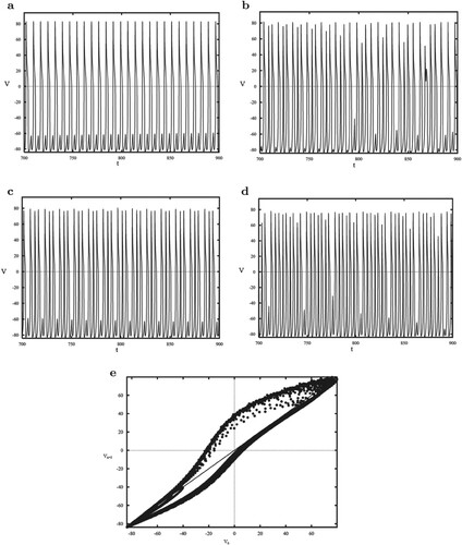
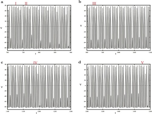
Re-examining the situation of $\varphi =1$, after some periodic spikes, the cell entered the bursting stage, including some small-amplitude slow oscillations (SAO) and a set of repetitive large-amplitude fast oscillations (LAO). As shown in Figure 5 (a), a bursting containing 9 spikes occurs after an SAO, and across another SAO, a 7-spiking bursting is found. Although the amplitude of the subsequent SAO has changed, the pattern of bursting with 7 spikes lasted 5 times, replaced by 5 continuous spikes, that remained for 13 times. Keep the time moving so that we get a new bursting with 7 spikes, followed by 5 LAOs between 2 SAOs, repeating 12 times. Finally, the time series ends with a 7-spike bursting when t is almost 1500. Thus it can be seen that the system has MMB with different number of LAOs.

Figure 5. Mixed-mode bursting at $\varphi =1$. The bursting part I contains 9 spikes and parts II, IV and V have 7 spikes. However, there are only 5 spikes in part III.

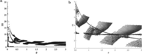
In general, ϕ has an important influence on the spiking transition. Figure 6 shows the bifurcations of the ISI series with respect to ϕ. It can be seen that in addition to the period-1 behaviour of the membrane potential, there also be multi-period behaviour.

Figure 6. (a) Bifurcations of the ISI series with increasing ϕ and (b) partial enlargement.

5. Dynamics of intracellular Ca${}^{2+}$

In addition to complex bursting, intracellular Ca${}^{2+}$ oscillation can also cause oscillatory hyperpolarization. As early as 1984, Ince et al. [25] declared that L cells (a mouse fibroblast cell line) and macrophages showed relatively low membrane potentials and slow oscillatory hyperpolarization. By injecting Ca${}^{2+}$ into P388D1 macrophages, Ca${}^{2+}$ -dependent oscillatory hyperpolarization of L cells and macrophages was reported, particularly, no oscillatory and single hyperpolarization reaction in Ca${}^{2+}$ -free medium, so it is deduced that Ca${}^{2+}$ was the activator of intracellular hyperpolarization.

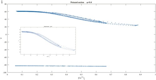
The last several sections of our paper mainly discuss the dynamic changes of $[{\mathrm{C}\mathrm{a}}^{2+}{]}_i$ and the induced hyperpolarization reaction based on the simulation and the parameters in Table A2. The $\left(\right[{\mathrm{I}\mathrm{P}}_3],A)$ bifurcation diagram is shown in Figure 7 (a), including bifurcation curves: the blue HB is for Hopf bifurcation, the green NS represents Neimark–Sacker bifurcation and the orange PD is period doubling bifurcation, where A is a variable to control the relative time scale between $[{\mathrm{C}\mathrm{a}}^{2+}{]}_i$ and h. It is obtained that the HB and NS bifurcation curves almost overlap for small A, and as $A\le 2$ PD bifurcation exists with the curve like a circle in $\left(\right[{\mathrm{I}\mathrm{P}}_3],A)$ plane. Figure 7(c) shows the one-parameter bifurcation diagram of $[{\mathrm{C}\mathrm{a}}^{2+}{]}_i$ oscillator depending on $\left[{\mathrm{I}\mathrm{P}}_3\right]$. The exact bifurcation points can be seen in the figure. The first Hopf bifurcation point (labelled by H) at $\left[{\mathrm{I}\mathrm{P}}_3\right]=0.153705$ is supercritical, bifurcating to a stable limit cycle whose period (Figure 7b) moves down according to $\left[{\mathrm{I}\mathrm{P}}_3\right]$. In the meantime a Neimark–Sacker (NS) point with parameter 0.1541724 and two period doubling (PD) points are seen in the figure, at $\left[{\mathrm{I}\mathrm{P}}_3\right]=0.1881808$ and 0.3962286 respectively. The limit point cycle (LPC) points declare a fold of the limit cycle manifold. A clearer display of 3-d space is shown in Figure 7 (d), where the coordinate h is the fraction of channels not inactivated by Ca${}^{2+}$.

Figure 7. Dynamics of $[{\mathrm{C}\mathrm{a}}^{2+}{]}_i$ oscillator. (a) $\left(\right[{\mathrm{I}\mathrm{P}}_3],A)$ bifurcation diagram includes HB (Hopf bifurcation), NS (Neimark-Sacker) and PD (period doubling) curves, represented by the blue, green and orange curves. (b) The period of the limit cycle bifurcating from Hopf bifurcation decreases with the increase of $\left[I{P}_3\right]$. (c-d) One-parameter bifurcation diagrams in 2-d and 3-d spaces, showing the bifurcation points: H ($\left[I{P}_3\right]=0.153705$), NS ($\left[I{P}_3\right]=0.1541724$) and PDs ($\left[I{P}_3\right]=0.1881808$ and 0.3962286). In the 3-d space, h is the fraction of channels not inactivated by Ca${}^{2+}$.

Choosing $\left[{\mathrm{I}\mathrm{P}}_3\right]=0.1539$ near the Hopf bifurcation, the trajectory of the model is located in the whirlpool caused by the stable limit cycle seen in Figure 8(a). Increasing $\left[{\mathrm{I}\mathrm{P}}_3\right]$ to 0.1542 crossing the NS bifurcation curve, a stable torus (Figure 8b) appears instead of the stable periodic orbit. When $\left[{\mathrm{I}\mathrm{P}}_3\right]=0.157$, the torus vanishes and more complex trajectories in Figure 8(c) arise standing for MMOs. Finally, for the PD bifurcation, we give the period-2 trajectory shown in Figure 8 (d), however, the period-3 orbit indicating the chaotic behaviour is not found, so we discuss the sensitive dependence of $[{\mathrm{C}\mathrm{a}}^{2+}{]}_i$ on the initial value, where the black and red orbits in Figure 7(e) demonstrate different initial value solutions with small disturbances. The distribution of the points on the Poincaré cross section h = 0.6 is also given in Figure 7 (f), forming a scatter plot of dispersion accumulation. These herald chaos.

Figure 8. (a–c) $\left(\right[{\mathrm{C}\mathrm{a}}^{2+}{]}_i,[{\mathrm{C}\mathrm{a}}^2+{]}_T)$ phase plot at $\left[{\mathrm{I}\mathrm{P}}_3\right]=0.1539,0.1542,0.157$: a whirlpool near the stable periodic solution, a stable torus and a complex solution corresponding to MMOs. (d) A period-2 solution near the PD bifurcation. (e–f) Chaotic characteristics checked by sensitive dependence on initial values and Poincaré cross section with the dispersion accumulation.

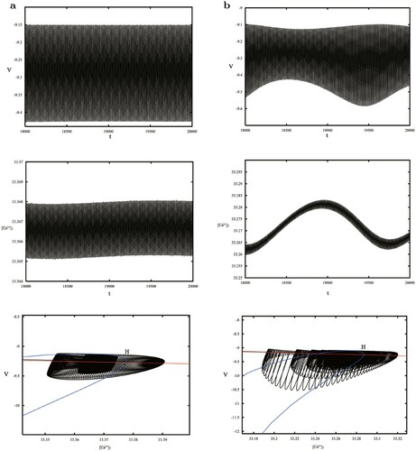
6. Hyperpolarizations related to $[{\mathrm{C}\mathrm{a}}^{2+}{]}_i$

Figure 8 has shown that the system has a stable $[{\mathrm{C}\mathrm{a}}^{2+}{]}_i$ periodic solution (the red curve in Figure 9a) at $\left[{\mathrm{I}\mathrm{P}}_3\right]=0.1539$. Again, the interaction of PM and ER oscillators comes out, whereas distinguished from the previous spiking or busting of PM oscillator, under the parameters in Table A2, the significantly low Ca${}^{2+}$ concentration is true and the oscillatory hyperpolarizations are evoked by periodic oscillation of $[{\mathrm{C}\mathrm{a}}^{2+}{]}_i$, that is, the membrane potential V is still negative for any time, the time series shown by the black curve in Figure 9 (a). The phase plots about V and $[{\mathrm{C}\mathrm{a}}^{2+}{]}_i$ with $\left[{\mathrm{I}\mathrm{P}}_3\right]=0.1539$ during different time periods are declared in Figure 9b–d, giving the change of periodic solutions in some time ranges.

Figure 9. (a) The periodic oscillation of $[{\mathrm{C}\mathrm{a}}^{2+}{]}_i$ (the red curve) and the oscillatory hyperpolarizations (the black curve) at $\left[{\mathrm{I}\mathrm{P}}_3\right]=0.1539$. (b–d) The phase plots during different time periods. (e) The pulse oscillation of $[{\mathrm{C}\mathrm{a}}^{2+}{]}_i$ (the red curve) and the peak-shaped solution of V (the black curve) with $\left[{\mathrm{I}\mathrm{P}}_3\right]=0.157$, local enlarged in (f). (g) The phase plot connecting oscillations with the different timescales.

Setting $\left[{\mathrm{I}\mathrm{P}}_3\right]=0.157$ demonstrates the periodic pulse oscillation of $[{\mathrm{C}\mathrm{a}}^{2+}{]}_i$ with the maximum concentration nearly up to 1, as shown in Figure 9(e) by the red curve, which leads to the peak-shaped hyperpolarizations (the black curve). The amplification of peak stage is shown in Figure 9(f) including the other two transient oscillations with large and small amplitudes, seen in Figure 9(g) combined with the pulse oscillation.

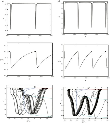
7. Torus canard-like behaviour

Canard refers to the solution of a singular perturbed system which contains both the attractive and repulsive parts. The one-dimensional isolated canard is also known as limit cycle canard [23], appearing in systems with Hopf bifurcation. In a singular perturbed system, canard passes through the fold point (or near the fold point) along the attraction part of the slow manifold, and then continues to form the periodic solution along the repulsive part of the slow manifold. Since the trajectories corresponding to these periodic solutions are similar in shape to canard in phase space in two-dimensional systems, these solutions are called canard solutions. According to the shape of periodic trajectory in phase space, it can be further divided into two cases: canard with head and without head. Similarly, a torus canard implies a family of attracting and repelling limit cycles of the fast system meets in a saddle-node, which is a quasiperiodic orbit from a torus bifurcation in the full system.

Changing the value of $\left[{\mathrm{I}\mathrm{P}}_3\right]$, the transition from the periodic hyperpolarization oscillation to the peak-shaped form is illustrated. Because of the restriction between $[{\mathrm{C}\mathrm{a}}^{2+}{]}_i$ and $[{\mathrm{C}\mathrm{a}}^{2+}{]}_T$, as well as the smallest timescale of $[{\mathrm{C}\mathrm{a}}^{2+}{]}_T$, we discuss the V oscillation with regard to $[{\mathrm{C}\mathrm{a}}^{2+}{]}_T$. With a description of the membrane potential, the periodic hyperpolarization orbits of V in Figure 10(a) at $\left[{\mathrm{I}\mathrm{P}}_3\right]=0.1539$ evolve depending on the small amplitude oscillation of $[{\mathrm{C}\mathrm{a}}^{2+}{]}_T$, embedded in a whirlpool in $\left(\right[{\mathrm{C}\mathrm{a}}^{2+}{]}_T,V)$ plane. $\left[{\mathrm{I}\mathrm{P}}_3\right]=0.1541$ close to the NS bifurcation point leads to the amplitude modulated (AM) oscillation, revealed in Figure 10(b), which tends to be like the headless torus canard. Continue to increase $\left[{\mathrm{I}\mathrm{P}}_3\right]$ to 0.157 and the peak-shaped solutions in Figure 10(c) appears analogous to a torus canard with head, whose transformation trend are similar to that of $[{\mathrm{C}\mathrm{a}}^{2+}{]}_T$, in other words, the peaks hold as a trough of $[{\mathrm{C}\mathrm{a}}^{2+}{]}_T$. At this time, the period of $[{\mathrm{C}\mathrm{a}}^{2+}{]}_T$ is slightly long, gives some sparse oscillation circles near H point. Further Figure 10(d) is the case at $\left[{\mathrm{I}\mathrm{P}}_3\right]=0.16$. The periods of V and $[{\mathrm{C}\mathrm{a}}^{2+}{]}_T$ decline in the meantime, forming a cluster of compact orbits.

Figure 10. (a) Periodic hyperpolarization oscillation at $\left[{\mathrm{I}\mathrm{P}}_3\right]=0.1539$; (b) AM oscillation similar to head less torus canard with $\left[{\mathrm{I}\mathrm{P}}_3\right]=0.1541$; (c) long-period peak-shaped orbit at $\left[{\mathrm{I}\mathrm{P}}_3\right]=0.157$ like torus canard; (d) short-period peak-shaped state at $\left[{\mathrm{I}\mathrm{P}}_3\right]=0.16$. Each subfigure contains three items: the wave plots of V and $[{\mathrm{C}\mathrm{a}}^{2+}{]}_T$, together with the trajectories of the whole system (the black curve) projected in $\left(\right[{\mathrm{C}\mathrm{a}}^{2+}{]}_T,V)$ space, where H is the Hopf bifurcation point, the red curve is the unstable equilibrium and the blue curves indicate the maximum and minimum of periodic orbits.

Taking $\left[{\mathrm{I}\mathrm{P}}_3\right]=0.16$ as an example, Figure 11(a) reveals the complete bifurcation diagram with stable (the black curves) and unstable (the red curve) equilibria, two Hopf bifurcation points ($[{\mathrm{C}\mathrm{a}}^{2+}{]}_T=30.78,67.17$ ), stable (the green curves) and unstable (the blue curves) periodic solutions. In detail, the upper H point bifurcates a periodic solution transforming from unstable one with large amplitude to stable one with small amplitude by the fold bifurcation of limit cycles, which meets the other limit cycle coming from the lower H point so that we can get a green closed curve in the middle of Figure 11 (a). We choose two different initial values of the full system close to the upper and lower H points respectively and find that the orbit with the initial value near the upper point fills about a half of the green circle, however, the second orbit is full of the circle, as shown in Figure 11 (b), that coincides with the time series in Figure 11(c), that is to say wherever the initial point is located at, the orbits distribute in the upper half of the circle.

Figure 11. (a) The complete bifurcation diagram of the system deleting $[{\mathrm{C}\mathrm{a}}^{2+}{]}_T$ dynamics at $\left[{\mathrm{I}\mathrm{P}}_3\right]=0.16$. There are two Hopf bifurcation points: $[{\mathrm{C}\mathrm{a}}^{2+}{]}_T=30.78,67.17$. The stable limit cycle from the upper point changed from a large-amplitude unstable one initially approaches the other orbit bifurcating from the lower point, forming a green circle. The black and red curves correspond to stable and unstable equilibrium. (b) The orbits of the whole system with initial values close to the two H points fill in the circle. (c) The orbits with different initial values go into the upper part of the circle.

8. Conclusion

The article focuses on a whole-cell model consisting of both membrane potential and Ca${}^{2+}$ oscillations. We show that the system has spiking and bursting behaviour as well as a transition from spiking to bursting. By adjusting the voltage gating of $K^{+}$, the relaxation oscillation and MMB can be exhibited. Changing the parameters, the variable $[{\mathrm{C}\mathrm{a}}^{2+}{]}_i$ presents the complex dynamics, generating the hyperpolarizations and torus canard-like pattern.

Specially, we first find that in the case of Table A1, whether or not ${\mathrm{I}\mathrm{P}}_3$ exists, the system always spikes, however, the status spiking to bursting happens when its concentration is not zero as Hopf bifurcation of V about $[{\mathrm{C}\mathrm{a}}^{2+}{]}_i$. The move of parameter ϕ results in the variety of solutions, i.e. bursting ($\varphi =12/s$), relaxation oscillation ($\varphi =0.01,0.001/s$), chaotic bursting ($\varphi =0.7$ to 1 with the step 0.1) and MMB ($\varphi =1$).

Parameters in Table A2 give the conclusion that Hopf, NS and PD bifurcations can be revealed according to $\left[{\mathrm{I}\mathrm{P}}_3\right]$, with a stable torus, period doubling solutions and chaos derived. In particular, taking specific values of $\left[{\mathrm{I}\mathrm{P}}_3\right]$ near the bifurcation points, it is shown that hyperpolarization oscillations and torus canard-like behaviour holds.

Mathematical models make it possible to study biological systems theoretically. We can use a relatively simple framework to guide experiments or verify hypotheses, and are not limited by experimental feasibility, cost, ethics and other factors. In the biological experiments of gonadotrophs, the dynamic behaviour of our model including bursting, relaxation oscillation, chaotic bursting and MMB has been found. Furthermore, for cardiomyocytes, it was found that Ca${}^{2+}$ oscillations would prolong the cells long action potential, leading to arrhythmia, and the dynamic mechanism of this phenomenon is canard [26]. Certainly, due to the complexity of the real biological system, the mathematical model cannot fully capture its characteristics or replace the biological experiment. The two should complement and confirm each other.

Authors' contributions

YL contributed to the conception of the study; XX performed the simulation; XX and YL contributed significantly to analysis and manuscript preparation; XX and DZ performed the data analyses and wrote the manuscript; YL and DZ helped perform the analysis with constructive discussions.

Acknowledgments

The authors want to thank G.B. Ermentrout, Lixia Duan and Qinghua Zhu for the helpful guidance of the manuscript.

Disclosure statement

No potential conflict of interest was reported by the author(s).

Additional information

Funding

The research is supported by National Natural Science Foundation of China (Nos. 11301263, 11701306, 11701275), the China Postdoctoral Science Foundation (No. 2018M630547), the Natural Science Fund Development Project by Nanjing Tech University, the Second Batch of High Level Demonstration Project for Sino-foreign Cooperative Education in Jiangsu, and the China Scholarship Council.

Appendix

Parameters in the paper are as follows:

Table

Parameter	Value	Parameter	Value	Parameter	Value
$C_m$	1 μM/${\mathrm{c}\mathrm{m}}^2$	$v_3$	$-20\mathrm{m}\mathrm{V}$	$K_d$	0.4 μM
$g_{\mathrm{C}\mathrm{a}}$	20 μS/${\mathrm{c}\mathrm{m}}^2$	$v_4$	30 mV	$K_{\mathrm{S}\mathrm{E}\mathrm{R}\mathrm{C}\mathrm{A}}$	0.2 μM
$g_K$	20 μS/${\mathrm{c}\mathrm{m}}^2$	$f_i$	0.01	$K_{\mathrm{P}\mathrm{M}\mathrm{C}\mathrm{A}}$	0.3 μM
$g_{\mathrm{K}\mathrm{C}\mathrm{a}}$	8 μS/${\mathrm{c}\mathrm{m}}^2$	$v_i$	4 pL	$V_{\mathrm{S}\mathrm{E}\mathrm{R}\mathrm{C}\mathrm{A}}$	480 aMol/s
$V_{\mathrm{C}\mathrm{a}}$	120 mV	L	1.48 pL/s	$V_{\mathrm{P}\mathrm{M}\mathrm{C}\mathrm{A}}$	400 aMol/s
$V_K$	$-85\mathrm{m}\mathrm{V}$	$P_{\mathrm{I}\mathrm{P}3\mathrm{R}}$	2960 pL/s	ϵ	0.01
$K_{\mathrm{K}\mathrm{C}\mathrm{a}}$	0.5 μM	$K_i$	0 μM	α	0.2(aMol$\cdot {\mathrm{c}\mathrm{m}}^2$)/nC
$v_1$	$-3\mathrm{m}\mathrm{V}$	$K_a$	0.4 μM	A	2/s
$v_2$	30 mV	σ	0.185

Table

Parameter	Value	Parameter	Value	Parameter	Value
$C_m$	20 μM/${\mathrm{c}\mathrm{m}}^2$	$v_3$	$-20\mathrm{m}\mathrm{V}$	$K_d$	0.4 μM
$g_{\mathrm{C}\mathrm{a}}$	20 μS/${\mathrm{c}\mathrm{m}}^2$	$v_4$	30 mV	$K_{\mathrm{S}\mathrm{E}\mathrm{R}\mathrm{C}\mathrm{A}}$	0.2 μM
$g_K$	20 μS/${\mathrm{c}\mathrm{m}}^2$	ϕ	12/s	$K_{\mathrm{P}\mathrm{M}\mathrm{C}\mathrm{A}}$	0.3 μM
$g_{\mathrm{K}\mathrm{C}\mathrm{a}}$	8.01 μS/${\mathrm{c}\mathrm{m}}^2$	$f_i$	0.01	$V_{\mathrm{S}\mathrm{E}\mathrm{R}\mathrm{C}\mathrm{A}}$	400 aMol/s
$V_{\mathrm{C}\mathrm{a}}$	120 mV	$v_i$	4 pL	$V_{\mathrm{P}\mathrm{M}\mathrm{C}\mathrm{A}}$	200 aMol/s
$V_{\mathrm{K}}$	-85 mV	L	0.37 pL/s	ϵ	0.01
$K_{\mathrm{K}\mathrm{C}\mathrm{a}}$	0.5μM	$P_{\mathrm{I}\mathrm{P}3\mathrm{R}}$	26640 pL/s	α	0.5 (aMol$\cdot {\mathrm{c}\mathrm{m}}^2$)/nC
$v_1$	$-3\mathrm{m}\mathrm{V}$	$K_i$	1 μM	A	0.5/s
$v_2$	30 mV	$K_a$	0.4 μM	σ	0.185

References

- M. Berridge, M. Bootman and P. Lipp, Calcium-a life and death signal, Nat. 395 (1998), pp. 645–648.
- P. Lipp, Nuclear calcium signalling by individual cytoplasmic calcium puffs, EMBO J. 16 (1997), pp. 7166–7173.
- L. Jaffe, Classes and mechanisms of calcium waves, Cell Calcium. 14 (1993), pp. 736–745.
- W. Li, J. Llopis, M. Whitney, G. Zlokarnik and R. Tsien, Cell-permeant caged insP3 ester shows that ca2+ spike frequency can optimize gene expression, Nat. 392 (1998), pp. 936–941.
- M. Berridge, Elementary and global aspects of calcium signalling, J. Physiol. 499 (1997), pp. 291–306.
- R. Dolmetsch, K. Xu and R. Lewis, Calcium oscillations increase the efficiency and specificity of gene expression, Nat. 392 (1998), pp. 933–936.
- A. Skupin and M. Falcke, Statistical analysis of calcium oscillations, Eur. Phys. J. Spec. Top. 187 (2010), pp. 231–240.
- G. Dupont, L. Combettes, G.S. Bird and J.W. Putney, Calcium oscillations, Cold Spring Harb. Perspectives Biol. 3 (2011), pp. a004226.
- A. Zhou, X. Liu and P. Yu, Bifurcation analysis on the effect of store-operated and receptor-operated calcium channels for calcium oscillations in astrocytes, Nonlin. Dyn. 97 (2019), pp. 1–16.
- C. Fall, Computational Cell Biology, Springer, New York, 2011.
- M. Berridge, P. Lipp and M. Bootman, The versatility and universality of calcium signalling, Nat. Rev. Mol. Cell Biol. 1 (2000), pp. 11–21.
- J. Sneyd, J.M. Han, L. Wang, J. Chen, X. Yang, A. Tanimura, M.J. Sanderson, V. Kirk and D.I. Yule, On the dynamical structure of calcium oscillations, Proc. Natl. Acad. Sci. 114 (2017), pp. 1456–1461.
- N. Pages, E. Vera-Sigenza, J. Rugis, V. Kirk, D.I. Yule and J. Sneyd, A model of Ca 2+ dynamics in an accurate reconstruction of parotid acinar cells, Bull. Math. Biol. 81 (2019), pp. 1394–1426.
- G Dupont, M Falcke, V Kirk and J Sneyd, Models of Calcium Signalling. Springer, Switzerland, 2016.
- S. Kingston and K. Thamilmaran, Bursting oscillations and mixed-mode oscillations in driven li e´nard system, Int. J. Bifurcat. Chaos. 27 (2017), pp. 1730025.
- Y. Sun, C. Ni, Y. Ge, H. Qian, Q. Ouyang and F. Li, Both cellular ATP level and ATP hydrolysis free energy determine energetically the calcium oscillation in pancreatic β-cell, 2018. arXiv:1811.11341.
- M. Falcke, R. Huerta, M.I. Rabinovich, H.D. Abarbanel, R.C. Elson and A.I. Selverston, Modeling observed chaotic oscillations in bursting neurons: the role of calcium dynamics and IP3, Biol. Cybern. 82 (2000), pp. 517–527.
- Z. L u¨, L. Chen and L. Duan, Bifurcation analysis of mixed bursting in the pre-B o¨tzinger complex, Appl. Math. Model. 67 (2019), pp. 234–251.
- E. Izhikevich, Neural excitability spiking and bursting, Int. J. Bifurcat. Chaos. 10 (2000), pp. 1171–1266.
- R. Straube, D. Flockerzi and M.J.B. Hauser, Sub-Hopf/fold-cycle bursting and its relation to (quasi-) periodic oscillations, J. Phys. Conf. Ser. 55 (2006), pp. 214–231.
- Z. Song and J. Xu, Bursting near bautin bifurcation in a neural network with delay coupling, Int. J. Neural Syst. 19 (2009), pp. 359–373.
- Y. Li, S. Stojilkovi c´, J. Keizer and J. Rinzel, Sensing and refilling calcium stores in an excitable cell, Biophys. J. 72 (1997), pp. 1080–1091.
- J. Burke, M. Desroches, A.M. Barry, T.J. Kaper and M.A. Kramer, A showcase of torus canards in neuronal bursters, J. Math. Neurosci. 2 (2012), pp. 3–32.
- H. Ju, A.B. Neiman and A.L. Shilnikov, Bottom-up approach to torus bifurcation in neuron models, Chaos: An Interdiscip. J. Nonlin. Sci. 28 (2018), pp. 106317.
- C. Ince, P.C. Leijh, J. Meijer, E. Van Bavel and D.L. Ypey, Oscillatory hyperpolarizations and resting membrane potentials of mouse fibroblast and macrophage cell lines, J. Physiol. 352 (1984), pp. 625–635.
- J. Kimrey, T. Vo and R. Bertram, Canard analysis reveals why a large Ca 2+ window current promotes early afterdepolarizations in cardiac myocytes, PLOS Comput. Biol. 16 (2020), pp. e1008341.