The state-dependent impulsive control for a general predator–prey model

Abstract

In this paper, a general predator–prey model with state-dependent impulse is considered. Based on the geometric analysis and Poincaré map or successor function, we construct three typical types of Bendixson domains to obtain some sufficient conditions for the existence of order-1 periodic solutions. At the same time, the existing domains are discussed with respect to the system parameters. Moreover, the Analogue of Poincaré Criterion is used to obtain the asymptotic stability of the periodic solutions. Finally, to illustrate the results, an example is presented and some numerical simulations are carried out.

Keywords:

• State-dependent impulse
• predator–prey model
• order-1 periodic solution
• Poincaré map
• successor function

2010 AMS Subject Classifications:

• 37N25
• 34A37
• 34C25

1. Introduction

Impulsive control is widely utilized in biology [6,7,25]. For instance, in the treatment of HIV-1 infection, the combination of vaccination and stimulation delays viral rebound following ART (Antiretroviral therapy) discontinuation [2,11,12]. Compared with the process of disease, the impact of taking drugs, vaccination and stimulation is short enough to be assumed that the therapy leads to an impulsive effect. Usually, from the economy point of view, the corresponding treatment is proposed to receive when the infected system reaches a critical state, on which the amount $CD{4}^{+}T$ decreases to 350 or 500 mm${}^{-3}$. Similarly, in the controlling of insects and other animals, to minimize damage to non-target organisms, and to preserve the environment, the integrated pest management (IPM) was introduced [3,17], which is a strategy that reduce pests to tolerable levels by releasing natural enemies, spraying pesticides, isolating or harvesting the pests when they reach a threshold. Likewise, in fishery industry, for the sake of ecological balance and maximum economic benefit, people usually take a sustainable strategy by harvesting and releasing according to the densities of certain species. For example, sometimes we need suppress the predator-fish by harvesting, and to stimulate the prey-fish by releasing, and other time it's just on the opposite purpose [9]. The discontinuity of human intervention leads to population changing very rapidly, which can be taken into account impulsive differential equations.

The impulsive differential equations have even been intensively studied in recent two decades, especially for state-dependent impulsive equations, which means the impulsive control takes place when a certain state is met [4,5,8,10–24,26]. However, because of the discontinuity of the system, the issue becomes more complicated but not less important than a continuous one. So it is still challenging to probe the dynamical properties of such systems.

In [21], Wang et al. consider an impulsive Kolmogorov predator–prey model with non-selective harvesting given by (1) $\left\{\begin{array}{ll}\left.\begin{array}{l}\frac{\mathrm{d}x}{\mathrm{d}t}=xF(x,y)\\ \frac{\mathrm{d}y}{\mathrm{d}t}=yG(x,y)\end{array}\right\},& x\ne h,\\ \left.\begin{array}{l}\mathrm{\Delta }x\left(t\right)=-px\left(t\right)\\ \mathrm{\Delta }y\left(t\right)=-qy\left(t\right)+\tau \end{array}\right\},& x=h,\end{array}\right.$(1) where $x\left(t\right)$ and $y\left(t\right)$ denote the densities of the prey and predator species at time t. Suppose one expects to perform an economical harvesting on the prey and predator (e.g. two kinds of food fish). When the density of prey increases to h, one harvests the prey and the predator at a rate p and q respectively. Because the reduction of prey may prevent predators from getting enough growth, and the harvesting on predator may also make it be on the verge of extinction, therefore to maintain the ecological balance among two populations and to obtain a sustainable economic benefit, one can release the predator on a scare of τ.

The authors incorporated two discriminants ${\mathrm{\Delta }}_1$ and ${\mathrm{\Delta }}_2$ to discuss the existence, non-existence and multiplicity as well as the stability of order-1 periodic solutions. Motivated by the work of [20,21], we consider the following state-dependent impulsive predator–prey population ecological model: (2) $\left\{\begin{array}{ll}\left.\begin{array}{l}\frac{\mathrm{d}x}{\mathrm{d}t}=xU(x,y)\\ \frac{\mathrm{d}y}{\mathrm{d}t}=yV\left(x\right)\end{array}\right\},& x\ne h,\\ \left.\begin{array}{l}\mathrm{\Delta }x\left(t\right)=-nx\left(t\right)\\ \mathrm{\Delta }y\left(t\right)=-my\left(t\right)+\tau \end{array}\right\},& x=h,\end{array}\right.$(2) where $x\left(t\right),y\left(t\right)$, h and τ are in the same meaning as those in (1(1) $\left\{\begin{array}{ll}\left.\begin{array}{l}\frac{\mathrm{d}x}{\mathrm{d}t}=xF(x,y)\\ \frac{\mathrm{d}y}{\mathrm{d}t}=yG(x,y)\end{array}\right\},& x\ne h,\\ \left.\begin{array}{l}\mathrm{\Delta }x\left(t\right)=-px\left(t\right)\\ \mathrm{\Delta }y\left(t\right)=-qy\left(t\right)+\tau \end{array}\right\},& x=h,\end{array}\right.$(1) ); n and m represent the rates at which the prey and the predator are harvested, respectively.

Assume that h is positive constant, and $n,m\in [0,1)$,$\tau \ge 0,F\in C^2({\mathbb{R}}^2,\mathbb{R}),G\in C(\mathbb{R},\mathbb{R})$. The initial value conditions satisfy (3) $0<x\left(0^{+}\right)=x_0^{+}<h,y\left(0^{+}\right)=y_0^{+}>0.$(3) Moreover, the following assumptions hold:

1. $U_x<0$, $U_y<0$, $V^{\prime }\left(x\right)>0$ for x>0.

2. There exist two positive numbers w<k such that $U(k,0)=0$ and $V\left(w\right)=0$, and $w>(1-n)h,k>h$.

In this paper, based on the theory of Bendixson domains established in [20,21], some results on the existence and stability of order-1 periodic solutions for system (2(2) $\left\{\begin{array}{ll}\left.\begin{array}{l}\frac{\mathrm{d}x}{\mathrm{d}t}=xU(x,y)\\ \frac{\mathrm{d}y}{\mathrm{d}t}=yV\left(x\right)\end{array}\right\},& x\ne h,\\ \left.\begin{array}{l}\mathrm{\Delta }x\left(t\right)=-nx\left(t\right)\\ \mathrm{\Delta }y\left(t\right)=-my\left(t\right)+\tau \end{array}\right\},& x=h,\end{array}\right.$(2) ) are established. Since the isolines of system (2(2) $\left\{\begin{array}{ll}\left.\begin{array}{l}\frac{\mathrm{d}x}{\mathrm{d}t}=xU(x,y)\\ \frac{\mathrm{d}y}{\mathrm{d}t}=yV\left(x\right)\end{array}\right\},& x\ne h,\\ \left.\begin{array}{l}\mathrm{\Delta }x\left(t\right)=-nx\left(t\right)\\ \mathrm{\Delta }y\left(t\right)=-my\left(t\right)+\tau \end{array}\right\},& x=h,\end{array}\right.$(2) ) are different from that of system (1(1) $\left\{\begin{array}{ll}\left.\begin{array}{l}\frac{\mathrm{d}x}{\mathrm{d}t}=xF(x,y)\\ \frac{\mathrm{d}y}{\mathrm{d}t}=yG(x,y)\end{array}\right\},& x\ne h,\\ \left.\begin{array}{l}\mathrm{\Delta }x\left(t\right)=-px\left(t\right)\\ \mathrm{\Delta }y\left(t\right)=-qy\left(t\right)+\tau \end{array}\right\},& x=h,\end{array}\right.$(1) ), the discriminants ${\mathrm{\Delta }}_1$ and ${\mathrm{\Delta }}_2$ are not always valid for system (2(2) $\left\{\begin{array}{ll}\left.\begin{array}{l}\frac{\mathrm{d}x}{\mathrm{d}t}=xU(x,y)\\ \frac{\mathrm{d}y}{\mathrm{d}t}=yV\left(x\right)\end{array}\right\},& x\ne h,\\ \left.\begin{array}{l}\mathrm{\Delta }x\left(t\right)=-nx\left(t\right)\\ \mathrm{\Delta }y\left(t\right)=-my\left(t\right)+\tau \end{array}\right\},& x=h,\end{array}\right.$(2) ). We classify the structure of Bendixson domains into three categories, and combine them with Poincaré maps and successor functions, which help us to obtain the existence and location of impulsive order-1 periodic solution(s). Further, by using the Analogue of Poincaré Criterion, the stability of the order-1 periodic solution for system (2(2) $\left\{\begin{array}{ll}\left.\begin{array}{l}\frac{\mathrm{d}x}{\mathrm{d}t}=xU(x,y)\\ \frac{\mathrm{d}y}{\mathrm{d}t}=yV\left(x\right)\end{array}\right\},& x\ne h,\\ \left.\begin{array}{l}\mathrm{\Delta }x\left(t\right)=-nx\left(t\right)\\ \mathrm{\Delta }y\left(t\right)=-my\left(t\right)+\tau \end{array}\right\},& x=h,\end{array}\right.$(2) ) is considered. In the last, we focus on the numerical simulations for the theory results.

2. Preliminaries

Let the impulse function be I, then $I(x,y)=\left(\right(1-n)x,(1-m)y+\tau )$. For the sake of simplicity, it is also denoted by $I\left(y\right)=(1-m)y+\tau$. Further, we denote the system without impulse that corresponding to (2(2) $\left\{\begin{array}{ll}\left.\begin{array}{l}\frac{\mathrm{d}x}{\mathrm{d}t}=xU(x,y)\\ \frac{\mathrm{d}y}{\mathrm{d}t}=yV\left(x\right)\end{array}\right\},& x\ne h,\\ \left.\begin{array}{l}\mathrm{\Delta }x\left(t\right)=-nx\left(t\right)\\ \mathrm{\Delta }y\left(t\right)=-my\left(t\right)+\tau \end{array}\right\},& x=h,\end{array}\right.$(2) ) by (4) $\left\{\begin{array}{l}\frac{\mathrm{d}x}{\mathrm{d}t}=xU(x,y),\\ \frac{\mathrm{d}y}{\mathrm{d}t}=yV\left(x\right).\end{array}\right.$(4) Let impulse set $M=\left\{\right(x,y)|y>0,x=h\}$ and image set $N=\left\{\right(x,y)|y>0,x=\underset{\_}{h}\}$, where $\underset{\_}{h}=(1-n)h+\tau$. Obviously $I\left(M\right)\subset N$. Let $O^{+}\left(Q\right)$ be the positive trajectory of the system (4(4) $\left\{\begin{array}{l}\frac{\mathrm{d}x}{\mathrm{d}t}=xU(x,y),\\ \frac{\mathrm{d}y}{\mathrm{d}t}=yV\left(x\right).\end{array}\right.$(4) ) starting from the point Q and let $O^{-}\left(Q\right)$ be a negative trajectory reaching the point Q. For any $Q(\underset{\_}{h},y)\in N$, if $O^{+}\left(Q\right)$ intersects with M for the first time at a point $\overline{Q}(h,\overline{y})$, and is consecutively mapped to $Q^{+}(\underset{\_}{h},y^{+})\in N$, then we define Poincaré map $P,P_N$ and successor function F as follows: (5) $P\left(Q\right)=\overline{Q},P_N\left(Q\right)=Q^{+},F\left(Q\right)=(I\circ P)\left(Q\right)-Q=Q^{+}-Q.$(5) where Q also represents its coordinate $y_Q$. For convenience, if a point A is above point B, that is $y_A>y_B$, then we write A>B. Obviously, $P_N=I^{o}P$, $F^{\mathrm{\prime }}\left(y\right)=(1-m)P^{\mathrm{\prime }}\left(y\right)-1.$

The geometric interpretation of Poincaré map $P,P_N$ and successor function F is shown in the Figure 1.

Figure 1. The geometric illustration for Poincaré maps P, $P_N$ and successor function F, where $P\left(Q\right)=\overline{Q},P_N\left(Q\right)=Q^{+},F\left(Q\right)=Q^{+}-Q$.

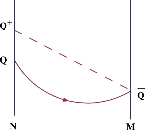
Definition 2.1

If $Q=Q^{+}$, that is $F\left(Q\right)=0$, then the ring formed by trajectory $Q\overline{Q}$ and line segment $\overline{Q}{Q}^{+}$ is called the order-1 periodic orbit.

It is known from the properties of U and V, for system (4(4) $\left\{\begin{array}{l}\frac{\mathrm{d}x}{\mathrm{d}t}=xU(x,y),\\ \frac{\mathrm{d}y}{\mathrm{d}t}=yV\left(x\right).\end{array}\right.$(4) ), that the existence and uniqueness of the solutions hold true, and the solutions are continuously dependent on and differentiable with respect to the initial value. It is also easy to verify that the solution of (4(4) $\left\{\begin{array}{l}\frac{\mathrm{d}x}{\mathrm{d}t}=xU(x,y),\\ \frac{\mathrm{d}y}{\mathrm{d}t}=yV\left(x\right).\end{array}\right.$(4) ) with a positive initial value must be positive.

Lemma 2.1

Under the Assumption $\left(A_1\right)$–$\left(A_2\right)$, the system (4(4) $\left\{\begin{array}{l}\frac{\mathrm{d}x}{\mathrm{d}t}=xU(x,y),\\ \frac{\mathrm{d}y}{\mathrm{d}t}=yV\left(x\right).\end{array}\right.$(4) ) has two unstable saddle points $E_0=(0,0)$, $E_1=(k,0)$ and an asymptotically stable node or focus $E_2=(w,y^{\ast })$, where $y^{\ast }$ is the solution of the equation $U(w,y)=0$. There is no positive periodic solution in the first quadrant for system (4(4) $\left\{\begin{array}{l}\frac{\mathrm{d}x}{\mathrm{d}t}=xU(x,y),\\ \frac{\mathrm{d}y}{\mathrm{d}t}=yV\left(x\right).\end{array}\right.$(4) ).

Proof.

Obviously, the point $(0,0)$ is an equilibrium. Since $U(k,0)=0$, the point $(k,0)$ is a boundary equilibrium of the system (4(4) $\left\{\begin{array}{l}\frac{\mathrm{d}x}{\mathrm{d}t}=xU(x,y),\\ \frac{\mathrm{d}y}{\mathrm{d}t}=yV\left(x\right).\end{array}\right.$(4) ). In addition, according to assumption $\left(A_1\right)$, the equation $U(x,y)=0$ determine an implicit function, named $y=\sigma \left(x\right)$. From the differential rule for implicit function, we have ${\sigma }^{\mathrm{\prime }}\left(x\right)=-\frac{U_x}{U_y}<0,$which means that the function $y=\sigma \left(x\right)$ is decreasing with x, and $\sigma \left(k\right)=0$ because of $U(k,0)=0$. Since $V\left(w\right)=0$ and w<k, so the curve of $y=\sigma \left(x\right)$ must intersect with the line x = w at the point $(w,y^{\ast })$, where $y^{\ast }$ is the solution of the equation $U(w,y)=0$. Hence $(w,y^{\ast })$ is a positive equilibrium of the system (4(4) $\left\{\begin{array}{l}\frac{\mathrm{d}x}{\mathrm{d}t}=xU(x,y),\\ \frac{\mathrm{d}y}{\mathrm{d}t}=yV\left(x\right).\end{array}\right.$(4) ).

The Jacobian matrix along the system (4(4) $\left\{\begin{array}{l}\frac{\mathrm{d}x}{\mathrm{d}t}=xU(x,y),\\ \frac{\mathrm{d}y}{\mathrm{d}t}=yV\left(x\right).\end{array}\right.$(4) ) is $J=\left[\begin{array}{ll}U(x,y)+x{U}_x& x{U}_y\\ y{V}^{\mathrm{\prime }}\left(x\right)& V\left(x\right)\end{array}\right].$Calculating the eigenvalues of the Jacobian matrix at $E_0=(0,0)$, $E_1=(k,0)$ and $E_2=(\omega ,y^{\ast })$, respectively, it is known that the equilibria $E_0$, $E_1$ are unstable saddle points and $E_2$ is an asymptotically stable node or focus.

Taking a Dulac function $D(x,y)=\frac{1}{xy}(x>0,y>0)$, we have $\frac{\mathrm{\partial }(D\cdot xU(x,y\left)\right)}{\mathrm{\partial }x}+\frac{\mathrm{\partial }(D\cdot yV(x\left)\right)}{\mathrm{\partial }y}=\frac{1}{y}{U}_x<0.$Therefore, the unique positive equilibrium point $E_2$ is globally asymptotically stable and there is no positive periodic solution in the first quadrant.

When $O^{+}\left(Q\right)\bigcap M\ne \mathrm{\Phi }$, we called the function P,$P_N$, F are well defined. Following the discussion in [21] and [20], we have

Lemma 2.2

If P,$P_N$, F are well defined on a non-tangent interval $[c,d]$(except the end point), then P, $P_N$, F are continuous on $[c,d]$.

Further similar analysis to Lemma 2.2 in [21] shows that the vector field of the system (4(4) $\left\{\begin{array}{l}\frac{\mathrm{d}x}{\mathrm{d}t}=xU(x,y),\\ \frac{\mathrm{d}y}{\mathrm{d}t}=yV\left(x\right).\end{array}\right.$(4) ) is counterclockwise.

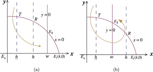
Let the isoline $y=\sigma \left(x\right)$ intersects with M and N at points $R=(h,y_R)$ and $T=(\underset{\_}{h},y_T)$ respectively. Then (6) $y_T=\sigma \left(\underset{\_}{h}\right),y_R=\sigma \left(h\right).$(6) Because of ${\sigma }^{\mathrm{\prime }}<0$ and $\underset{\_}{h}<h$, we have $y_R<y_T$. The possible location of impulse set, image set, isolines and related characterized points is shown in Figure 2.

Figure 2. The possible location of impulse section, image section, isoclines and some characterized points: (a)$\underset{\_}{h}<h<x^{\ast }=w$; (b) $\underset{\_}{h}<x^{\ast }<h$.

Definition 2.2

For system (2(2) $\left\{\begin{array}{ll}\left.\begin{array}{l}\frac{\mathrm{d}x}{\mathrm{d}t}=xU(x,y)\\ \frac{\mathrm{d}y}{\mathrm{d}t}=yV\left(x\right)\end{array}\right\},& x\ne h,\\ \left.\begin{array}{l}\mathrm{\Delta }x\left(t\right)=-nx\left(t\right)\\ \mathrm{\Delta }y\left(t\right)=-my\left(t\right)+\tau \end{array}\right\},& x=h,\end{array}\right.$(2) ), suppose a domain D is composed of impulse set M, image set N, trajectory $L_1$ and $L_2$, and satisfies

1. there is no singularity in D;

2. the trajectory $L_1$ intersects with N and M at A and $\overline{A}$ successively; the trajectory $L_2$ intersects with N, M at B and $\overline{B}$ successively;

3. line segments AB and $\overline{A}\overline{B}$ have no tangent points with the trajectory of the system (4(4) $\left\{\begin{array}{l}\frac{\mathrm{d}x}{\mathrm{d}t}=xU(x,y),\\ \frac{\mathrm{d}y}{\mathrm{d}t}=yV\left(x\right).\end{array}\right.$(4) ) except for the end points.

If $A>B\Rightarrow \overline{A}>\overline{B}$, then D is called a parallel rectangular domain (see Figure 3a).

Figure 3. The illustration for three categories of Bendexion domain: (a) parallel domain; (b) sub-parallel domain; (c) semi-ring domain.

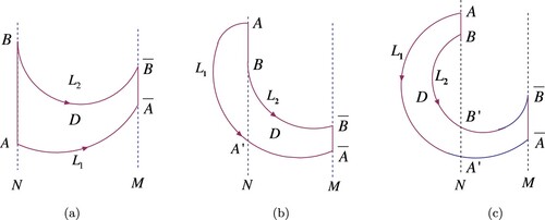
If $A>B\Rightarrow \overline{A}<\overline{B}$, and $L_2$ is tangent to N at B, then D is called a sub-parallel rectangular domain (see Figure 3b).

If $A>B\Rightarrow \overline{A}<\overline{B}$, $L_1$ intersects with N at A and $A^{\mathrm{\prime }}$ successively, and $L_2$ intersects with N at B and $B^{\mathrm{\prime }}$ successively, and $L_2$ is tangent to M at $B^{\mathrm{\prime }}$, then D is called a semi-circle domain (see Figure 3c).

Lemma 2.3

[20,21]

For parallel and sub-parallel domains, if F is defined on the non-tangent interval $[A,B]\subset N$ and such that $F\left(A\right)F\left(B\right)<0$, then there is an order-1 periodic solution starting from $C\in AB$. For semi-ring domains, if $P_N\left(AB\right)\subset AB$ or $P_N\left(A^{\mathrm{\prime }}{B}^{\mathrm{\prime }}\right)\subset AB$, then there is an order-1 periodic solution starting from AB. If $P_N\left(AB\right)\subset A^{\mathrm{\prime }}{B}^{\mathrm{\prime }}$ or $P_N\left(A^{\mathrm{\prime }}{B}^{\mathrm{\prime }}\right)\subset A^{\mathrm{\prime }}{B}^{\mathrm{\prime }}$, then there is an order-1 periodic solution starting from $A^{\mathrm{\prime }}{B}^{\mathrm{\prime }}$. If $P_N\left(AB\right)\subseteq B{B}^{\prime }$ or $P_N\left(A^{\prime }{B}^{\prime }\right)\subseteq B{B}^{\prime }$, then there is no order-1 periodic solution in D (see Figure 3).

3. Main results

Let $(\underset{\_}{h},\tau )\triangleq Q_{\tau }$, $(\underset{\_}{h},\frac{\tau }{m})\triangleq Q_m$.

Lemma 3.1

For any $\overline{Q}(h,\overline{y})\in M$, if $\overline{y}>\frac{\tau }{m}$, then $Q_m<I\left(\overline{Q}\right)<\overline{Q}$; if $\overline{y}<\frac{\tau }{m}$, then $\overline{Q}<I\left(\overline{Q}\right)<Q_m$.

Proof.

Obviously, $I\left(y\right)=(1-m)y+\tau \Rightarrow I\left(\frac{\tau }{m}\right)=\frac{\tau }{m}$. Assume that $\overline{y}>\frac{\tau }{m}$. On the one hand, we have $I\left(\overline{y}\right)=(1-m)\overline{y}+\tau >(1-m)\frac{\tau }{m}+\tau =\frac{\tau }{m}$. On the other hand, $I\left(\overline{y}\right)=(1-m)\overline{y}+\tau =\overline{y}+(\tau -m\overline{y})<\overline{y}$. Thus $\frac{\tau }{m}<I\left(\overline{y}\right)<\overline{y}$, which means $Q_m<I\left(\overline{Q}\right)<\overline{Q}$. Similarly, when $\overline{y}<\frac{\tau }{m}$, we have $\overline{y}<I\left(\overline{y}\right)<\frac{\tau }{m}$, that is $\overline{Q}<I\left(\overline{Q}\right)<Q_m$.

Further, if $F\left(Q_{\tau }\right)$ is well defined, then (7) $F\left(Q_{\tau }\right)=(1-m)y_{{\overline{Q}}_{\tau }}+\tau -\tau >0.$(7) Next, we discuss the existence and location of order-1 periodic solutions of the system (2(2) $\left\{\begin{array}{ll}\left.\begin{array}{l}\frac{\mathrm{d}x}{\mathrm{d}t}=xU(x,y)\\ \frac{\mathrm{d}y}{\mathrm{d}t}=yV\left(x\right)\end{array}\right\},& x\ne h,\\ \left.\begin{array}{l}\mathrm{\Delta }x\left(t\right)=-nx\left(t\right)\\ \mathrm{\Delta }y\left(t\right)=-my\left(t\right)+\tau \end{array}\right\},& x=h,\end{array}\right.$(2) ) under the case $\underset{\_}{h}<h<x^{\ast }=w$ and $\underset{\_}{h}<x^{\ast }<h$, respectively.

3.1. $\underset{\_}{h}<h<x^{\ast }=w$

In this case, for any $Q\in N$, $F\left(Q\right)$ is well defined since $E_2(w,y^{\ast })$ is globally asymptotically stable.

Theorem 3.1

Assume $\left(A_1\right)$–$\left(A_2\right)$ hold and $\tau >0$. Then there must exist a positive order-1 periodic solution for system (2(2) $\left\{\begin{array}{ll}\left.\begin{array}{l}\frac{\mathrm{d}x}{\mathrm{d}t}=xU(x,y)\\ \frac{\mathrm{d}y}{\mathrm{d}t}=yV\left(x\right)\end{array}\right\},& x\ne h,\\ \left.\begin{array}{l}\mathrm{\Delta }x\left(t\right)=-nx\left(t\right)\\ \mathrm{\Delta }y\left(t\right)=-my\left(t\right)+\tau \end{array}\right\},& x=h,\end{array}\right.$(2) ).

Proof.

To specify the structure and location of the order-1 periodic solution and probe the effect of parameter m and τ, we discuss case by case.

Case 1. $\frac{\tau }{m}>y_T$.

$\left(i\right)$ $F\left(T\right)>0$. The domain formed by trajectory $T\overline{T}$ and $T^{+}{\overline{T}}^{+}$, segments $T{T}^{+}$ and $\overline{T}{\overline{T}}^{+}$ is sub-parallel. It follows from the structure of the trajectories of system (2(2) $\left\{\begin{array}{ll}\left.\begin{array}{l}\frac{\mathrm{d}x}{\mathrm{d}t}=xU(x,y)\\ \frac{\mathrm{d}y}{\mathrm{d}t}=yV\left(x\right)\end{array}\right\},& x\ne h,\\ \left.\begin{array}{l}\mathrm{\Delta }x\left(t\right)=-nx\left(t\right)\\ \mathrm{\Delta }y\left(t\right)=-my\left(t\right)+\tau \end{array}\right\},& x=h,\end{array}\right.$(2) ) and the monotonic increasing of impulse function I that $F\left(T^{+}\right)<0$. Thus $F\left(T\right)F\left(T^{+}\right)<0$. According to Lemma 2.3, there is an order-1 periodic solution in this sub-parallel domain.

$\left(ii\right)$ $F\left(T\right)<0$. Because $F\left(Q_{\tau }\right)$ is well defined, the domain composed of trajectories $T\overline{T}$ and $Q_{\tau }{\overline{Q}}_{\tau }$, segments $T{Q}_{\tau }$ and $\overline{T}{\overline{Q}}_{\tau }$ is a parallel one. It follows from (7(7) $F\left(Q_{\tau }\right)=(1-m)y_{{\overline{Q}}_{\tau }}+\tau -\tau >0.$(7) ) that $F\left(T\right)F\left(Q_{\tau }\right)<0$, which implies that there is a positive order-1 periodic solution starting from the segment $T{Q}_{\tau }$.

Case 2. $0<\frac{\tau }{m}\le y_T$.

Take the trajectory as a graph of a function, then $O^{+}\left(T\right)$ is decreasing with respect to x for $x<x^{\ast }=w$. Therefore $\overline{T}<T$. It follows from Lemma 3.1 that $I\left(\overline{T}\right)<T$ no matter $\frac{\tau }{m}\le y_{\overline{T}}$ or $\frac{\tau }{m}>y_{\overline{T}}$, and hence $F\left(T\right)<0$. Moreover $F\left(Q_{\tau }\right)>0$, which leads to $F\left(T\right)F\left(Q_{\tau }\right)<0$. So in the parallel domain composed of trajectories $Q_{\tau }{\overline{Q}}_{\tau }$, $T\overline{T}$ and segments $Q_{\tau }T$ and $\overline{Q_{\tau }}\overline{T}$, there is a positive order-1 periodic solution initiating from the segment $Q_{\tau }T$.

Theorem 3.2

Suppose that $\tau =0$. Then there is a semi-trivial periodic solution $\left(X\right(t),0)$, where $\underset{\_}{h}\le X\left(t\right)\le h$.

Proof.

When $\underset{\_}{h}<x<h<w$, $O^{+}\left(Q\right)$ is decreasing for any Q<T, and it follows that $\overline{Q}<Q$. If $\tau =0$, then $F\left(Q\right)=(1-m)\overline{Q}-Q<0$ for Q<T. Moreover, similar to the discussion of Lemma 2.2 in [21], we have (8) $\begin{array}{rl}{F}^{\prime }\left(Y\right)& =(1-m)\exp \left({\int }_{\underset{\_}{h}}^h\frac{zU(z,y(z,Y\left)\right)V\left(z\right)-zV\left(z\right)y(z,Y)U_y(z,y(z,Y\left)\right)}{\left(zU\right(z,y(z,Y)){)}^2}\mathrm{d}z-1,\right.\\ & Y<y_T.\end{array}$(8) From the assumption $\left(A_1\right)$–$\left(A_2\right)$, it gives $F^{\prime }\left(Y\right)<0$ for $Y<y_T$. Thus for the successor function F, both $F\left(Q\right)<0$ and $F^{\prime }\left(Q\right)<0$ are satisfied for Q<T. Since 0<m<1 and the solutions of system (4(4) $\left\{\begin{array}{l}\frac{\mathrm{d}x}{\mathrm{d}t}=xU(x,y),\\ \frac{\mathrm{d}y}{\mathrm{d}t}=yV\left(x\right).\end{array}\right.$(4) ) are positive with positive initial value. Henceforth, $\underset{ϵ\to 0^{+}}{lim}F\left(ϵ\right)=0$ holds true because of the continuity of F.

Remark 3.1

In fact, even since $\underset{\_}{h}<x^{\ast }<h$, the inequality $F\left(T\right)<0$ is always true under the case that $F\left(T\right)$ is well defined and $\tau =0$. In view of the uniqueness of the solution, the trajectory $Q^{+}\left(T\right)$ intersects with the isoline on the right side of M, therefore $\overline{T}<T$ holds, which means $F\left(T\right)<0$.

When m = 0, the result is similar to the case $\frac{\tau }{m}>y_T$.

Corollary 3.1

Suppose m = 0. Then the following statements are true. (i) If $F\left(T\right)>0$, then there is an order-1 periodic solution initiating above T. (ii) If $F\left(T\right)<0$, then the order-1 periodic solution is starting from $Q_{\tau }T$, which is below T.

3.2. $\underset{\_}{h}<x^{\ast }<h$

In this case, $F\left(T\right)$ may be not well defined.

If $F\left(T\right)$ is well defined, $F\left(Q\right)$ is defined for any $Q\in N$. Similar to the proof of Theorem 3.1, there must exist an order-1 periodic solution for system (2(2) $\left\{\begin{array}{ll}\left.\begin{array}{l}\frac{\mathrm{d}x}{\mathrm{d}t}=xU(x,y)\\ \frac{\mathrm{d}y}{\mathrm{d}t}=yV\left(x\right)\end{array}\right\},& x\ne h,\\ \left.\begin{array}{l}\mathrm{\Delta }x\left(t\right)=-nx\left(t\right)\\ \mathrm{\Delta }y\left(t\right)=-my\left(t\right)+\tau \end{array}\right\},& x=h,\end{array}\right.$(2) ).

If $F\left(T\right)$ is not well defined (it is only possible when $\underset{\_}{h}<x^{\ast }<h$), we only consider the case that $O^{-}\left(R\right)\cap N\ne \mathrm{\Phi }$ and there are at least two intersection points, because the impulse control is hardly valid when there is unique or no intersection[20,21]. Let $\begin{array}{rl}{R}_{-}& =max\left\{R_k|O^{+}\right(R_k)\bigcap M=R,R_k<T\},\\ R^{-}& =min\left\{R_k|O^{+}\right(R_k)\bigcap M=R,R_k>T\}.\end{array}$From Lemma 2.3, we have the following theorems.

Theorem 3.3

Suppose that $\frac{\tau }{m}\ge y_{R^{-}}$, $I\left(R\right)>R^{-}$ and $P_N\left(R^{+}\right)>R^{-}$ hold. Then there is an order-1 periodic solution starting from segment $R^{-}{R}^{+}$, which lies in the semi-ring domain.

Proof.

Obviously, under the conditions given by the theorem, $P_N\left(R_{-}{R}^{+}\right)\subset R_{-}{R}^{+}$ holds true. It follows from Lemma 2.3 that there is an order-1 periodic solution in the semi-ring domain, which is composed of trajectories $R_{-}{\overline{R}}_{-}$, $R^{+}{\overline{R}}^{+}$ and segments $R_{-}{R}^{+}$ and ${\overline{R}}_{-}{\overline{R}}^{+}$.

Theorem 3.4

Suppose that $\tau \ge y_{R_{-}}$ and $\frac{\tau }{m}<y_{R^{-}}$ hold. Then the system (2(2) $\left\{\begin{array}{ll}\left.\begin{array}{l}\frac{\mathrm{d}x}{\mathrm{d}t}=xU(x,y)\\ \frac{\mathrm{d}y}{\mathrm{d}t}=yV\left(x\right)\end{array}\right\},& x\ne h,\\ \left.\begin{array}{l}\mathrm{\Delta }x\left(t\right)=-nx\left(t\right)\\ \mathrm{\Delta }y\left(t\right)=-my\left(t\right)+\tau \end{array}\right\},& x=h,\end{array}\right.$(2) ) has no positive periodic solution.

Proof.

Since $\tau \ge y_{R_{-}}$, we have $I\left(y_R\right)=(1-m)y_R+\tau >\tau \ge y_{R_{-}}$. From Lemma 3.1, no matter $\frac{\tau }{m}<y_R$ or $\frac{\tau }{m}>y_R$, the inequality $I\left(R\right)<R^{-}$ can be obtained from $\frac{\tau }{m}<y_{R^{-}}$ and $y_R<y_T<y_{R^{-}}$. The trajectories starting from the points below $R_{-}$ on N are all mapped onto segment $R_{-}{R}^{-}$ under the effect of impulse, so the trajectory initiating on $R_{-}{R}^{-}$ will no longer reach M, which are determined by system (4(4) $\left\{\begin{array}{l}\frac{\mathrm{d}x}{\mathrm{d}t}=xU(x,y),\\ \frac{\mathrm{d}y}{\mathrm{d}t}=yV\left(x\right).\end{array}\right.$(4) ). From Lemma 2.3, there is no positive periodic solution for system (4(4) $\left\{\begin{array}{l}\frac{\mathrm{d}x}{\mathrm{d}t}=xU(x,y),\\ \frac{\mathrm{d}y}{\mathrm{d}t}=yV\left(x\right).\end{array}\right.$(4) ), so does for system (2(2) $\left\{\begin{array}{ll}\left.\begin{array}{l}\frac{\mathrm{d}x}{\mathrm{d}t}=xU(x,y)\\ \frac{\mathrm{d}y}{\mathrm{d}t}=yV\left(x\right)\end{array}\right\},& x\ne h,\\ \left.\begin{array}{l}\mathrm{\Delta }x\left(t\right)=-nx\left(t\right)\\ \mathrm{\Delta }y\left(t\right)=-my\left(t\right)+\tau \end{array}\right\},& x=h,\end{array}\right.$(2) ).

Theorem 3.5

Suppose $0<\tau <y_{R_{-}}$ holds. If $I\left(R\right)<R_{-}$, then there is an order-1 periodic solution which departures from segment $Q_{\tau }{R}_{-}$. Specifically, if $F\left(Q_m\right)<0$, then there is an order-1 periodic solution initiating from segment $Q_{\tau }{Q}_m$.

Proof.

Equation (7(7) $F\left(Q_{\tau }\right)=(1-m)y_{{\overline{Q}}_{\tau }}+\tau -\tau >0.$(7) ) gives $F\left(Q_{\tau }\right)>0$. Since $I\left(R\right)<R_{-}$, that is $F\left(R\right)<0$, and hence $F\left(\tau \right)F\left(R\right)<0$ holds. It is known from Lemma 2.3 that there is an order-1 periodic solution initiating from the segment $Q_{\tau }{R}_{-}$. Specifically, if $F\left(Q_m\right)<0$, then $F\left(Q_{\tau }\right)F\left(Q_m\right)<0$. Therefore there is an positive order-1 periodic solution initiating from segment $Q_{\tau }{Q}_m$.

Remark 3.2

Theorems 3.2–3.4 present the sufficient conditions for the existence or non-existence of order-1 periodic solutions to system (2(2) $\left\{\begin{array}{ll}\left.\begin{array}{l}\frac{\mathrm{d}x}{\mathrm{d}t}=xU(x,y)\\ \frac{\mathrm{d}y}{\mathrm{d}t}=yV\left(x\right)\end{array}\right\},& x\ne h,\\ \left.\begin{array}{l}\mathrm{\Delta }x\left(t\right)=-nx\left(t\right)\\ \mathrm{\Delta }y\left(t\right)=-my\left(t\right)+\tau \end{array}\right\},& x=h,\end{array}\right.$(2) ). We have not established the existence conditions of order-1 periodic solution when $I\left(R\right)>R_{-}$ and $0<\tau <y_{R_{-}}$, the simulations show that there maybe exist or not exist a positive order-1 periodic solution.

Remark 3.3

When $F\left(T\right)$ is well defined, the results are the same as that under the case $\underset{\_}{h}<h<x^{\ast }$.

Theorem 3.6

Suppose $\tau =0$ and $F\left(T\right)$ be not well defined. Then there is a semi-trivial order-1 periodic solution under the case $I\left(R\right)<R_{-}$, and when $I\left(R\right)>R_{-}$, there maybe exist an positive order-1 periodic solution.

Proof.

Since $O^{-}\left(R\right)\cap N\ne set$, we have $F\left(ϵ\right)$ is well defined for $ϵ<R_{-}$. Further, $\underset{ϵ\to 0^{+}}{lim}F\left(ϵ\right)=0$ holds true, which means there exists a semi-trivial order-1 periodic solution. When $\underset{\_}{h}<x^{\ast }<h$, from Equation (8(8) $\begin{array}{rl}{F}^{\prime }\left(Y\right)& =(1-m)\exp \left({\int }_{\underset{\_}{h}}^h\frac{zU(z,y(z,Y\left)\right)V\left(z\right)-zV\left(z\right)y(z,Y)U_y(z,y(z,Y\left)\right)}{\left(zU\right(z,y(z,Y)){)}^2}\mathrm{d}z-1,\right.\\ & Y<y_T.\end{array}$(8) ), the inequality $F^{\prime }\left(Q\right)<0$ does not necessarily hold for $Q<R_{-}$. Therefore, when $I\left(R\right)>R_{-}$, there maybe exist an positive order-1 periodic solution besides the semi-trivial periodic solution.

Corollary 3.2

Suppose m = 0 and $F\left(T\right)$ be well defined. Then the following statements are true. (i) If $F\left(T\right)>0$, then there is an order-1 periodic solution initiating above T. (ii) If $F\left(T\right)<0$, the order-1 periodic solution is initiating from $Q_{\tau }T$, which is below T.

Corollary 3.3

Suppose that m = 0 and $F\left(T\right)$ be not well defined. (i) If $I\left(R\right)>R^{-}$ and $P_N\left(R^{+}\right)>R^{-}$, there is an order -1 periodic solution starting above $R^{-}$. (ii) If $I\left(R\right)<R^{-}$, there is an order -1 periodic solution starting from $Q_{\tau }{R}_{-}$.

Remark 3.4

When $\underset{\_}{h}<x^{\ast }<h$, $F\left(T\right)$ maybe or not well defined. If $F\left(T\right)$ is well defined, for any $Q<T\in N$,$F\left(Q\right)$ is well defined. If $F\left(T\right)$ is not well defined, for any $Q<R_{-}\in N$, $F\left(Q\right)$ is well defined. When $\underset{\_}{h}<h<x^{\ast }$, the trajectory $O^{+}\left(Q\right)$ is decreasing with x on $[\underset{\_}{h},h]$, however, it is not necessarily decreasing on $[\underset{\_}{h},h]$ under the case $\underset{\_}{h}<x^{\ast }<h$. Hence, it is still possible that there is a point Q such that $(1-m)y_{\overline{Q}}+\tau >y_Q$, that is, $F\left(Q\right)>0$. If $F\left(T\right)$ is well defined and $F\left(T\right)<0$, then it is still possible that there is a positive order-1 periodic solution starting from the segment QT. If $F\left(T\right)$ is not well defined and $I\left(R\right)<R_{-}$, that is, $F\left(R_{-}\right)<0$, then there may exist a positive order-1 periodic solution which initiating from the segment $Q{R}_{-}$.

Next, we summarize the results in two tables as follows, which are listed according to whether $F\left(T\right)$ is well defined, where the symbol ‘par.’ and ‘semi-tri.’ are the abbreviations of ‘parallel’ and ‘semi-trivial’. The check mark ‘$✓$’ indicates the claim is true(see Table 1 and Table 2).

Table 1. The existence and location of order-1 periodic solution when $F\left(T\right)$ is well defined.

${\displaystyle \frac{\mathit{\tau }}{\mathit{m}}}$	$\mathit{F}\mathbf{\left(}\mathit{T}\mathbf{\right)}$	Others	Initiating location	Existing domain
$\frac{\tau }{m}>y_T(m=0)$	$>0$	$/$	above T	Sub-par.
	$<0$	$F\left(\tau \right)>0\left(✓\right)$	segment $Q_{\tau }T$	Par.
$0<\frac{\tau }{m}\le y_T$	$<0\left(✓\right)$	$F\left(\tau \right)>0\left(✓\right)$	segment $Q_{\tau }T$	Par.
$\tau =0$	$<0$(✓)	$\underset{ϵ\to 0}{lim}F\left(ϵ\right)=0\left(✓\right)$	x-axis $(\underset{\_}{h},0)$	Semi-tri.

Table 2. The existence and location of order-1 periodic solution when $F\left(T\right)$ is not well defined.

$\tau ,m$	$I\left(R\right)$	Others	Initiating location	Existing domain
$\frac{\tau }{m}\ge y_{R^{-}}$ $(m=0)$	$I\left(R\right)>R^{-}$	$P_N\left(R^{+}\right)>R^{-}$	above $R^{-}$	Semi-ring
$\tau \ge y_{R_{-}}$ and $\frac{\tau }{m}<y_{R^{-}}$	$I\left(R\right)<R^{-}$ (✓)	$/$	$/$	None
$0<\tau <y_{R_{-}}$ $(m=0)$	$I\left(R\right)<R_{-}$	$F\left(\tau \right)>0$	segment $Q_{\tau }{R}_{-}$	Par.
$\tau =0$	$I\left(R\right)<R_{-}$	$\underset{ϵ\to 0}{lim}F\left(ϵ\right)=0$	x-axis $(\underset{\_}{h},0)$	Semi-tri.
	$I\left(R\right)>R_{-}$	$\mathrm{\exists }Q<R_{-}$,$F\left(Q\right)<0$	segment $Q{R}_{-}$	Par.

4. Stability of the order-1 positive periodic solution

Consider the general plane state-dependent impulsive differential system (9) $\left\{\begin{array}{lll}\frac{\mathrm{d}x}{\mathrm{d}t}=P(x,y),& \frac{\mathrm{d}y}{\mathrm{d}t}=Q(x,y),& \mathrm{i}\mathrm{f}\varphi (x,y)\ne 0,\\ \mathrm{\Delta }x=I_1(x,y),& \mathrm{\Delta }y=I_2(x,y),& \mathrm{i}\mathrm{f}\varphi (x,y)=0,\end{array}\right.$(9) where $P(x,y)$, $Q(x,y)$ is continuously differentiable, $\mathrm{\Phi }(x,y)$ is a smooth function and $\mathrm{\nabla }\mathrm{\Phi }\ne 0$.

Lemma 4.1

Analogue of Poincaré Criterion [1,8,15].

If $|{\mu }_1|<1$, then the order-1 periodic solution of system (9) is orbitally asymptotically stable, where (10) $\begin{array}{rl}{\mu }_1& =\prod _{j=1}^n{\kappa }_j\exp \left\{{\int }_0^{\omega }\left[\frac{\mathrm{\partial }P\left(\xi \left(t\right),\eta \left(t\right)\right)}{\mathrm{\partial }x}+\frac{\mathrm{\partial }Q\left(\xi \left(t\right),\eta \left(t\right)\right)}{\mathrm{\partial }y}\right]\mathrm{d}t\right\},\end{array}$(10) (11) $\begin{array}{rl}{\kappa }_j& =\frac{\left(\frac{\mathrm{\partial }{I}_2}{\mathrm{\partial }y}\frac{\mathrm{\partial }\varphi }{\mathrm{\partial }x}-\frac{\mathrm{\partial }{I}_2}{\mathrm{\partial }x}\frac{\mathrm{\partial }\varphi }{\mathrm{\partial }y}+\frac{\mathrm{\partial }\varphi }{\mathrm{\partial }x}\right)P_{+}+\left(\frac{\mathrm{\partial }{I}_1}{\mathrm{\partial }x}\frac{\mathrm{\partial }\varphi }{\mathrm{\partial }y}-\frac{\mathrm{\partial }{I}_1}{\mathrm{\partial }y}\frac{\mathrm{\partial }\varphi }{\mathrm{\partial }x}+\frac{\mathrm{\partial }\varphi }{\mathrm{\partial }y}\right)Q_{+}}{\frac{\mathrm{\partial }\varphi }{\mathrm{\partial }x}P+\frac{\mathrm{\partial }\varphi }{\mathrm{\partial }y}Q},\end{array}$(11) and $P,Q,\frac{\mathrm{\partial }{I}_1}{\mathrm{\partial }x},\frac{\mathrm{\partial }{I}_1}{\mathrm{\partial }y},\frac{\mathrm{\partial }{I}_2}{\mathrm{\partial }x},\frac{\mathrm{\partial }{I}_2}{\mathrm{\partial }y},\frac{\mathrm{\partial }\varphi }{\mathrm{\partial }x},\frac{\mathrm{\partial }\varphi }{\mathrm{\partial }y}$ are calculated at the point $\left(\xi \right({\tau }_j),\eta ({\tau }_j\left)\right)$, $P_{+},$ and $Q_{+}$ are calculated at the point $\left(\xi \right({\tau }_j^{+}),\eta ({\tau }_j^{+}\left)\right)$, and ${\tau }_j$ is the time of the jth jump.

Theorem 4.1

Let $\left(X\right(t),Y(t\left)\right)$ be an order-1 ω-periodic solution of the system (2(2) $\left\{\begin{array}{ll}\left.\begin{array}{l}\frac{\mathrm{d}x}{\mathrm{d}t}=xU(x,y)\\ \frac{\mathrm{d}y}{\mathrm{d}t}=yV\left(x\right)\end{array}\right\},& x\ne h,\\ \left.\begin{array}{l}\mathrm{\Delta }x\left(t\right)=-nx\left(t\right)\\ \mathrm{\Delta }y\left(t\right)=-my\left(t\right)+\tau \end{array}\right\},& x=h,\end{array}\right.$(2) ). If $|{\mu }_1|<1$, then $\left(X\right(t),Y(t\left)\right)$ is orbitally asymptotically stable, where (12) $|{\mu }_1|=\frac{(1-m)Y\left(\omega \right)}{(1-m)Y\left(\omega \right)+\tau }\cdot \exp \left\{{\int }_0^{\omega }\left[\frac{-Y{U}_{y}V}{U}\right]{|}_{\left(X\right(t),Y(t\left)\right)}\mathrm{d}t\right\}<1.$(12)

Proof.

Suppose $\left(X\right(t),Y(t\left)\right)$ intersects with M, N at the point $O(h,Y(\omega \left)\right)$ and $O^{+}(\underset{\_}{h},Y({\omega }^{+}\left)\right)$, respectively, where $Y\left({\omega }^{+}\right)=(1-m)Y\left(\omega \right)+\tau$. Corresponding to system (9(9) $\left\{\begin{array}{lll}\frac{\mathrm{d}x}{\mathrm{d}t}=P(x,y),& \frac{\mathrm{d}y}{\mathrm{d}t}=Q(x,y),& \mathrm{i}\mathrm{f}\varphi (x,y)\ne 0,\\ \mathrm{\Delta }x=I_1(x,y),& \mathrm{\Delta }y=I_2(x,y),& \mathrm{i}\mathrm{f}\varphi (x,y)=0,\end{array}\right.$(9) ), we have $P(x,y)=xU(x,y)$, $Q(x,y)=yV\left(x\right)$, $\mathrm{\Phi }(x,y)=x-h$, and $I_1(x,y)=-nx$ and $I_2(x,y)=-my+\tau$. Therefore $\begin{array}{rl}& \frac{\mathrm{\partial }P}{\mathrm{\partial }x}=U(x,y)+x{U}_x,\frac{\mathrm{\partial }Q}{\mathrm{\partial }y}=V\left(x\right),\frac{\mathrm{\partial }{I}_1}{\mathrm{\partial }x}=-n,\frac{\mathrm{\partial }{I}_2}{\mathrm{\partial }y}=-m,\\ & \frac{\mathrm{\partial }\varphi }{\mathrm{\partial }x}=1,\frac{\mathrm{\partial }{I}_1}{\mathrm{\partial }y}=\frac{\mathrm{\partial }{I}_2}{\mathrm{\partial }x}=\frac{\mathrm{\partial }\varphi }{\mathrm{\partial }y}=0.\end{array}$It follows that (13) $\begin{array}{rl}{\kappa }_1& =\frac{\left(\frac{\mathrm{\partial }{I}_2}{\mathrm{\partial }y}\frac{\mathrm{\partial }\varphi }{\mathrm{\partial }x}-\frac{\mathrm{\partial }{I}_2}{\mathrm{\partial }x}\frac{\mathrm{\partial }\varphi }{\mathrm{\partial }y}+\frac{\mathrm{\partial }\varphi }{\mathrm{\partial }x}\right)P_{+}+\left(\frac{\mathrm{\partial }{I}_1}{\mathrm{\partial }x}\frac{\mathrm{\partial }\varphi }{\mathrm{\partial }y}-\frac{\mathrm{\partial }{I}_1}{\mathrm{\partial }y}\frac{\mathrm{\partial }\varphi }{\mathrm{\partial }x}+\frac{\mathrm{\partial }\varphi }{\mathrm{\partial }y}\right)Q_{+}}{\frac{\mathrm{\partial }\varphi }{\mathrm{\partial }x}P+\frac{\mathrm{\partial }\varphi }{\mathrm{\partial }y}Q}\\ & =\frac{(1-m)P^{+}}{P}.\end{array}$(13) Moreover, we have (14) $\begin{array}{rl}{\int }_0^{\omega }\frac{\mathrm{\partial }P(X,Y)}{\mathrm{\partial }X}\mathrm{d}t& ={\int }_0^{\omega }\left[U\right(X,Y)+X{U}_x(X,Y\left)\right]\mathrm{d}t\\ & ={\int }_{\underset{\_}{h}}^h\frac{1}{X}\mathrm{d}X+{\int }_0^{\omega }X{U}_x(X,Y)\mathrm{d}t=\ln \frac{h}{\underset{\_}{h}}+{\int }_0^{\omega }X{U}_x(X,Y)\mathrm{d}t\end{array}$(14) and (15) ${\int }_0^{\omega }\frac{\mathrm{\partial }Q(X,Y)}{\mathrm{\partial }Y}\mathrm{d}t={\int }_0^{\omega }V\left(X\right)\mathrm{d}t={\int }_{Y\left({\omega }^{+}\right)}^{Y\left(\omega \right)}\frac{1}{Y}\mathrm{d}Y=\ln \frac{Y\left(\omega \right)}{Y\left({\omega }^{+}\right)}.$(15) Further, the last items of (14(14) $\begin{array}{rl}{\int }_0^{\omega }\frac{\mathrm{\partial }P(X,Y)}{\mathrm{\partial }X}\mathrm{d}t& ={\int }_0^{\omega }\left[U\right(X,Y)+X{U}_x(X,Y\left)\right]\mathrm{d}t\\ & ={\int }_{\underset{\_}{h}}^h\frac{1}{X}\mathrm{d}X+{\int }_0^{\omega }X{U}_x(X,Y)\mathrm{d}t=\ln \frac{h}{\underset{\_}{h}}+{\int }_0^{\omega }X{U}_x(X,Y)\mathrm{d}t\end{array}$(14) ) give (16) $\begin{array}{rl}{\int }_0^{\omega }X{U}_x(X,Y)\mathrm{d}t& ={\int }_0^{\omega }\frac{X\left[U_x\right(X,Y)+U_y(X,Y\left)\frac{\mathrm{d}Y}{\mathrm{d}X}\right]}{XU(X,Y)}\dot{X}\left(t\right)\mathrm{d}t-{\int }_0^{\omega }\frac{U_y(X,Y)}{U(X,Y)}\dot{Y}\left(t\right)\mathrm{d}t\\ & ={\int }_{\underset{\_}{h}}^h\frac{\mathrm{d}U(X,Y(X\left)\right)}{U(X,Y(X\left)\right)}-{\int }_0^{\omega }\frac{U_y(X,Y)}{U(X,Y)}YV\left(X\right)\mathrm{d}t\\ & =\ln \frac{U(h,Y(\omega \left)\right)}{U(\underset{\_}{h},Y({\omega }^{+})}-{\int }_0^{\omega }\frac{U_y(X,Y)}{U(X,Y)}YV\left(X\right)\mathrm{d}t.\end{array}$(16) Hence, it follows from (14(14) $\begin{array}{rl}{\int }_0^{\omega }\frac{\mathrm{\partial }P(X,Y)}{\mathrm{\partial }X}\mathrm{d}t& ={\int }_0^{\omega }\left[U\right(X,Y)+X{U}_x(X,Y\left)\right]\mathrm{d}t\\ & ={\int }_{\underset{\_}{h}}^h\frac{1}{X}\mathrm{d}X+{\int }_0^{\omega }X{U}_x(X,Y)\mathrm{d}t=\ln \frac{h}{\underset{\_}{h}}+{\int }_0^{\omega }X{U}_x(X,Y)\mathrm{d}t\end{array}$(14) )–(16(16) $\begin{array}{rl}{\int }_0^{\omega }X{U}_x(X,Y)\mathrm{d}t& ={\int }_0^{\omega }\frac{X\left[U_x\right(X,Y)+U_y(X,Y\left)\frac{\mathrm{d}Y}{\mathrm{d}X}\right]}{XU(X,Y)}\dot{X}\left(t\right)\mathrm{d}t-{\int }_0^{\omega }\frac{U_y(X,Y)}{U(X,Y)}\dot{Y}\left(t\right)\mathrm{d}t\\ & ={\int }_{\underset{\_}{h}}^h\frac{\mathrm{d}U(X,Y(X\left)\right)}{U(X,Y(X\left)\right)}-{\int }_0^{\omega }\frac{U_y(X,Y)}{U(X,Y)}YV\left(X\right)\mathrm{d}t\\ & =\ln \frac{U(h,Y(\omega \left)\right)}{U(\underset{\_}{h},Y({\omega }^{+})}-{\int }_0^{\omega }\frac{U_y(X,Y)}{U(X,Y)}YV\left(X\right)\mathrm{d}t.\end{array}$(16) ) that (17) $\begin{array}{rl}\exp \left\{{\int }_0^{\omega }\left[\frac{\mathrm{\partial }P\left(X,Y\right)}{\mathrm{\partial }X}+\frac{\mathrm{\partial }Q\left(X,Y\right)}{\mathrm{\partial }Y}\right]\mathrm{d}t\right\}& =\exp \left\{\ln \frac{h}{\underset{\_}{h}}+\ln \frac{U(h,Y(\omega \left)\right)}{U(\underset{\_}{h},Y({\omega }^{+}\left)\right)}+\ln \frac{Y\left(\omega \right)}{Y\left({\omega }^{+}\right)}\right.\\ & \left.-{\int }_0^{\omega }\frac{U_y(X,Y)}{U(X,Y)}YV\left(X\right)\mathrm{d}t\right\}\\ & =\frac{h}{\underset{\_}{h}}\cdot \frac{U(h,Y(\omega \left)\right)}{U(\underset{\_}{h},Y({\omega }^{+})}\\ & \cdot \exp \left\{-{\int }_0^{\omega }\left[\frac{U_y(X,Y)}{U(X,Y)}YV\left(X\right)\right]\mathrm{d}t\right\}.\end{array}$(17) Therefore, according to (12(12) $|{\mu }_1|=\frac{(1-m)Y\left(\omega \right)}{(1-m)Y\left(\omega \right)+\tau }\cdot \exp \left\{{\int }_0^{\omega }\left[\frac{-Y{U}_{y}V}{U}\right]{|}_{\left(X\right(t),Y(t\left)\right)}\mathrm{d}t\right\}<1.$(12) ), (13(13) $\begin{array}{rl}{\kappa }_1& =\frac{\left(\frac{\mathrm{\partial }{I}_2}{\mathrm{\partial }y}\frac{\mathrm{\partial }\varphi }{\mathrm{\partial }x}-\frac{\mathrm{\partial }{I}_2}{\mathrm{\partial }x}\frac{\mathrm{\partial }\varphi }{\mathrm{\partial }y}+\frac{\mathrm{\partial }\varphi }{\mathrm{\partial }x}\right)P_{+}+\left(\frac{\mathrm{\partial }{I}_1}{\mathrm{\partial }x}\frac{\mathrm{\partial }\varphi }{\mathrm{\partial }y}-\frac{\mathrm{\partial }{I}_1}{\mathrm{\partial }y}\frac{\mathrm{\partial }\varphi }{\mathrm{\partial }x}+\frac{\mathrm{\partial }\varphi }{\mathrm{\partial }y}\right)Q_{+}}{\frac{\mathrm{\partial }\varphi }{\mathrm{\partial }x}P+\frac{\mathrm{\partial }\varphi }{\mathrm{\partial }y}Q}\\ & =\frac{(1-m)P^{+}}{P}.\end{array}$(13) ), (14(14) $\begin{array}{rl}{\int }_0^{\omega }\frac{\mathrm{\partial }P(X,Y)}{\mathrm{\partial }X}\mathrm{d}t& ={\int }_0^{\omega }\left[U\right(X,Y)+X{U}_x(X,Y\left)\right]\mathrm{d}t\\ & ={\int }_{\underset{\_}{h}}^h\frac{1}{X}\mathrm{d}X+{\int }_0^{\omega }X{U}_x(X,Y)\mathrm{d}t=\ln \frac{h}{\underset{\_}{h}}+{\int }_0^{\omega }X{U}_x(X,Y)\mathrm{d}t\end{array}$(14) ) and (17(17) $\begin{array}{rl}\exp \left\{{\int }_0^{\omega }\left[\frac{\mathrm{\partial }P\left(X,Y\right)}{\mathrm{\partial }X}+\frac{\mathrm{\partial }Q\left(X,Y\right)}{\mathrm{\partial }Y}\right]\mathrm{d}t\right\}& =\exp \left\{\ln \frac{h}{\underset{\_}{h}}+\ln \frac{U(h,Y(\omega \left)\right)}{U(\underset{\_}{h},Y({\omega }^{+}\left)\right)}+\ln \frac{Y\left(\omega \right)}{Y\left({\omega }^{+}\right)}\right.\\ & \left.-{\int }_0^{\omega }\frac{U_y(X,Y)}{U(X,Y)}YV\left(X\right)\mathrm{d}t\right\}\\ & =\frac{h}{\underset{\_}{h}}\cdot \frac{U(h,Y(\omega \left)\right)}{U(\underset{\_}{h},Y({\omega }^{+})}\\ & \cdot \exp \left\{-{\int }_0^{\omega }\left[\frac{U_y(X,Y)}{U(X,Y)}YV\left(X\right)\right]\mathrm{d}t\right\}.\end{array}$(17) ), we have $\begin{array}{rl}|{\mu }_1|& =\frac{(1-m)P_{+}}{P}\cdot \frac{h}{\underset{\_}{h}}\frac{Y\left(\omega \right)}{Y\left({\omega }^{+}\right)}\frac{U(h,Y(\omega \left)\right)}{U(\underset{\_}{h},Y(\omega \left)\right)}\cdot \exp \left\{-{\int }_0^{\omega }\left[\frac{U_y(X,Y)}{U(X,Y)}YV\left(X\right)\right]\mathrm{d}t\right\}\\ & =\frac{(1-m)Y\left(\omega \right)}{(1-m)Y\left(\omega \right)+\tau }\cdot \exp \left\{-{\int }_0^{\omega }\left[\frac{U_{y}YV}{U}\right]{|}_{\left(X\right(t),Y(t\left)\right)}\mathrm{d}t\right\}<1.\end{array}$According to Lemma 4.1, the order-1 periodic solution $\left(X\right(t),Y(t\left)\right)$ is orbitally asymptotically stable.

Remark 4.1

If $h<x^{\ast }$ and $F\left(T\right)<0$, then there exists an order-1 periodic solution $\left(X\right(t),Y(t\left)\right)$, which must be orbitally asymptotically stable, in view of $U>0,U_y\le 0$ and V <0, Y >0 for $Y\left({\omega }^{+}\right)<y_T$, and hence $|{\mu }_1|<1$.

5. Example and simulations

Consider the state-dependent impulsive differential system (18) $\left\{\begin{array}{ll}\left.\begin{array}{l}\frac{\mathrm{d}x}{\mathrm{d}t}=rx\left(1-\frac{x}{k}\right)-\text{β}xy\\ \frac{\mathrm{d}y}{\mathrm{d}t}=y(\text{β}x-\alpha )\end{array}\right\},& x<h,\\ \left.\begin{array}{l}\mathrm{\Delta }x=-nx\left(t\right)\\ \mathrm{\Delta }y=-my\left(t\right)+\tau \end{array}\right\},& x=h.\end{array}\right.$(18) Obviously, corresponding to system (2(2) $\left\{\begin{array}{ll}\left.\begin{array}{l}\frac{\mathrm{d}x}{\mathrm{d}t}=xU(x,y)\\ \frac{\mathrm{d}y}{\mathrm{d}t}=yV\left(x\right)\end{array}\right\},& x\ne h,\\ \left.\begin{array}{l}\mathrm{\Delta }x\left(t\right)=-nx\left(t\right)\\ \mathrm{\Delta }y\left(t\right)=-my\left(t\right)+\tau \end{array}\right\},& x=h,\end{array}\right.$(2) ), we have $U(x,y)=r-\frac{r}{k}x-\text{β}y,V\left(x\right)=\text{β}x-\alpha ,U_x=-\frac{r}{k},U_y=-\text{β},V^{\prime }\left(x\right)=\text{β}.$From $V\left(x\right)=0$, it follows that $w=\frac{\mu }{\text{β}}$. It is not difficult to figure out $(x^{\ast },y^{\ast })=\left(\frac{\alpha }{\text{β}},\frac{r}{\text{β}}\left(1-\frac{\alpha }{k\text{β}}\right)\right),y_T=\frac{r}{\text{β}}\left(1-\frac{\underset{\_}{h}}{k}\right),y_R=\frac{r}{\text{β}}\left(1-\frac{h}{k}\right).$If k>h and $(1-n)h<\frac{\mu }{\text{β}}$, then the assumptions $\left(A_1\right)$ and $\left(A_2\right)$ hold.

In the following, some simulations are carried out by Matlab software, which are somewhat corresponding to Table 1 and Table 2.

5.1. $F\left(T\right)$ is well defined

Taking the parameters r = 1, k = 10, $\text{β}=0.025$, a = 0.188, n = 0.3 and h = 5.5, the computation shows that $(x^{\ast },y^{\ast })=(7.52,9.92)$, $\underset{\_}{h}=3.85$, $y_T=24.6$ and $y_{\overline{T}}=15.8055$, which means $\underset{\_}{h}<h<x^{\ast }$.

Let $\tau =15$ and m = 0. Then $\frac{\tau }{m}=150>y_T$ and $F\left(T\right)=5.73>0$ are satisfied. As can be seen from Figure 4(a) that there is an order-1 periodic solution in a sub-parallel domain. Let $\tau =7$ and m = 0.1. Then we have $\frac{\tau }{m}=70>y_T$ and $F\left(T\right)=-2.269<0$. There is an order-1 periodic solution initiating below T, which is in a parallel domain (Figure 4b). If $\tau =2$ and m = 0.1, then the condition $0<\frac{\tau }{m}=20<y_T$ holds true, it can be seen from Figure 4(c) that there exists an order-1 periodic solution in a parallel domain. Let $\tau =0$ and m = 0.1. It is known from Figure 4(d) that there is a semi-trivial periodic solution in the system.

Figure 4. The order-1 periodic solution of system (18(18) $\left\{\begin{array}{ll}\left.\begin{array}{l}\frac{\mathrm{d}x}{\mathrm{d}t}=rx\left(1-\frac{x}{k}\right)-\text{β}xy\\ \frac{\mathrm{d}y}{\mathrm{d}t}=y(\text{β}x-\alpha )\end{array}\right\},& x<h,\\ \left.\begin{array}{l}\mathrm{\Delta }x=-nx\left(t\right)\\ \mathrm{\Delta }y=-my\left(t\right)+\tau \end{array}\right\},& x=h.\end{array}\right.$(18) ) under the case $\underset{\_}{h}<h<x^{\ast }$, where r = 1, k = 10, $\text{β}=0.025$, a = 0.188, n = 0.3,h = 5.5. (a) m = 0, $\tau =15$ such that $\frac{\tau }{m}>y_T$ and $F\left(T\right)>0$; (b)m = 0.1, $\tau =7$ such that $\frac{\tau }{m}>y_T$ and $F\left(T\right)<0$; (c) m = 0.1, $\tau =2$ such that $0<\frac{\tau }{m}<y_T$ and $F\left(T\right)<0$; (d) when $\tau =0$ and m = 0.1, there is a semi-trivial periodic solution.

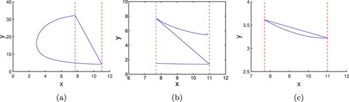
When $\underset{\_}{h}<x^{\ast }<h$, $F\left(T\right)$ may be well defined or not well defined.

Let r = 0.5, k = 15, $\text{β}=0.025$, a = 0.165, m = 0.03, n = 0.428, h = 7 be fixed, the calculation shows that $\underset{\_}{h}=4.004$, $y_T=14.661$ and $y_{\overline{T}}=9.9286$, which means $F\left(T\right)$ is well defined. Compared with Figure 1, Figure 2 illustrates the existence of the order-1 periodic solutions which are the same as $h<x^{\ast }$.

Figure 1 and Figure 2 show that there must exist an positive order-1 periodic solution for system (2(2) $\left\{\begin{array}{ll}\left.\begin{array}{l}\frac{\mathrm{d}x}{\mathrm{d}t}=xU(x,y)\\ \frac{\mathrm{d}y}{\mathrm{d}t}=yV\left(x\right)\end{array}\right\},& x\ne h,\\ \left.\begin{array}{l}\mathrm{\Delta }x\left(t\right)=-nx\left(t\right)\\ \mathrm{\Delta }y\left(t\right)=-my\left(t\right)+\tau \end{array}\right\},& x=h,\end{array}\right.$(2) ) under the case $F\left(T\right)$ is well defined and $\tau >0$.

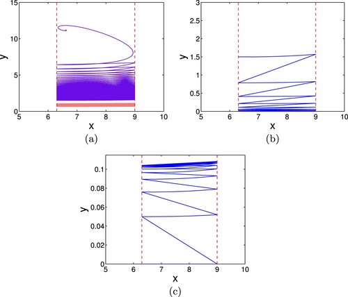
5.2. $F\left(T\right)$ is not well defined

If $F\left(T\right)$ is not well defined, then $\underset{\_}{h}<x^{\ast }<h$.

Taking r = 0.5, k = 15, $\text{β}=0.025$, a = 0.27, n = 0.3, m = 0.5 and h = 11, then $\underset{\_}{h}=7.7$, $(x^{\ast },y^{\ast })=(10.8,5.6)$, which means $\underset{\_}{h}<x^{\ast }<h$. The calculation gives $y_T=9.7333$, $y_R=5.333$ and $F\left(T\right)$ is not well defined. Further, $y_{R_{-}}=6.808$ and $y_{R^{-}}=18.875$ are obtained.

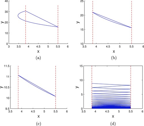
Let $\tau =30$. Then $\frac{\tau }{m}=60\ge y_{R^{-}}$, $I\left(R\right)=y_{R^{+}}=32.6665>y_{R^{-}}$ and $P_N\left(R^{+}\right)=32.089>y_{R^{-}}$ are satisfied. It can be seen from Figure 6(a) that there is an order-1 periodic solution which locates in a semi-ring domain. Take $\tau =7$, then $\tau >y_{R_{-}}$ and $\frac{\tau }{m}=14<y_{R^{-}}$ hold. As can be seen from Figure 6(b) that there does not exist periodic solution because the trajectories of the system ultimately approach the equilibrium $(x\ast ,y\ast )$. While $\tau =2$, we can verify that $0<\tau <y_{R_{-}}$, $I\left(y_R\right)=y_{R^{+}}=4.6665<y_{R_{-}}$ and $F\left(\tau \right)=0.91715>0$. We can see from Figure 6(c) that an order-1 periodic solution exists.

Figure 5. The existence of order-1 periodic solution of system (5.1) when $\underset{\_}{h}<x^{\ast }<h$ and $F\left(T\right)$ is well defined, where r = 0.5, k = 15, $\text{β}=0.025$, a = 0.165, m = 0.03, n = 0.428 and h = 7. (a) $\tau =7$ such that $\frac{\tau }{m}>y_T$ and $F\left(T\right)>0$; (b) $\tau =1$ such that $\frac{\tau }{m}>y_T$ and $F\left(T\right)<0$; (c) $\tau =0.05$ such that $0<\frac{\tau }{m}\le y_T$; (d) $\tau =0$.

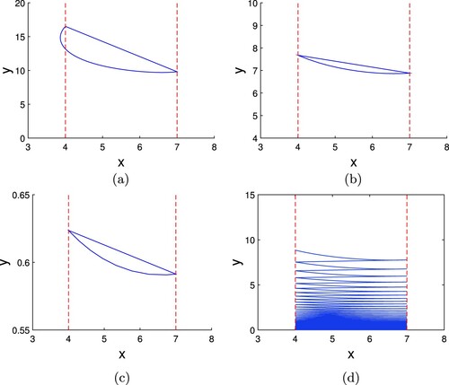
Figure 6. The existence of order-1 periodic solution of system (18(18) $\left\{\begin{array}{ll}\left.\begin{array}{l}\frac{\mathrm{d}x}{\mathrm{d}t}=rx\left(1-\frac{x}{k}\right)-\text{β}xy\\ \frac{\mathrm{d}y}{\mathrm{d}t}=y(\text{β}x-\alpha )\end{array}\right\},& x<h,\\ \left.\begin{array}{l}\mathrm{\Delta }x=-nx\left(t\right)\\ \mathrm{\Delta }y=-my\left(t\right)+\tau \end{array}\right\},& x=h.\end{array}\right.$(18) ) when $\underset{\_}{h}<x^{\ast }<h$ and $F\left(T\right)$ is not well defined, where r = 0.5,k = 15,$\text{β}=0.025$,a = 0.27, n = 0.3, m = 0.5 and h = 11. (a) $\tau =30$ such that $\frac{\tau }{m}\ge y_{R^{-}}$,$I\left(R\right)>R^{-}$ and $P_N\left(R^{+}\right)>R^{-}$; (b) $\tau =7$ such that $\tau \ge Y_{R_{-}}$ and $\frac{\tau }{m}<y_{R^{-}}$; (c) $\tau =2$ such that $0<\tau <Y_{R_{-}}$,$I\left(R\right)<R_{-}$.

Let r = 0.5, k = 15, $\text{β}=0.025$, a = 0.165, n = 0.3 and h = 9 be fixed. Then we have $\underset{\_}{h}=6.35$, $y_R=8$ and $y_{R_{-}}=6.325$. Take $\tau =0$ and m = 0.04, then $I\left(R\right)=7.68>6.3=R_{-}$. When $(x_0,y_0)=(6.3,0.5)$, it can be seen from Figure 7(a) that the system has a limit cycle. Changing the initial value $(x_0,y_0)=(6.3,1.5)$, the trajectory approaches the equilibrium $E_2$ after finite times of impulse impact. Let $\tau =0$ and m = 0.5. Then $I\left(R\right)=4<6.325=R_{-}$, and the system has a semi-trivial order-1 periodic solution (see Figure 7b). Given a small $\tau =0.05$, even since the initial value of y is zero, there is still a positive order-1 periodic solution (see Figure 7c).

Figure 7. The existence of periodic solution of system (18(18) $\left\{\begin{array}{ll}\left.\begin{array}{l}\frac{\mathrm{d}x}{\mathrm{d}t}=rx\left(1-\frac{x}{k}\right)-\text{β}xy\\ \frac{\mathrm{d}y}{\mathrm{d}t}=y(\text{β}x-\alpha )\end{array}\right\},& x<h,\\ \left.\begin{array}{l}\mathrm{\Delta }x=-nx\left(t\right)\\ \mathrm{\Delta }y=-my\left(t\right)+\tau \end{array}\right\},& x=h.\end{array}\right.$(18) ) when $\underset{\_}{h}<x^{\ast }<h$ and $F\left(T\right)$ is not well defined, where r = 0.5, k = 15, $\text{β}=0.025$, a = 0.165, n = 0.3 and h = 9. (a) $\tau =0$, m = 0.04, such that $I\left(R\right)>R_{-}$, $(x_0,y_0)$ is taken by $(6.3,5.5)$ and $(6.3,0.5)$,respectively; (b) $\tau =0$, m = 0.5, such that $I\left(R\right)<R_{-}$, $(x_0,y_0)=(6.3,1.5)$, and $\underset{ϵ\to 0^{+}}{lim}F\left(ϵ\right)=0$; (c) $\tau =0.05$, m = 0.5, such that $I\left(R\right)<R_{-}$, where $(x_0,y_0)=(6.3,0)$.

From Figure 7, it can be seen that the existence of periodic solutions depends on the initial values, parameters $m,\tau$ and the structure of the system without impulse. Moreover, Figure 7(b) and Figure 7(c) show that a small τ can stimulate a positive order-1 periodic solution.

5.3. Stability of the order-1 periodic solution

Let $\left(X\right(t),Y(t\left)\right)$ be an order-1 ω-periodic solution of the system (18(18) $\left\{\begin{array}{ll}\left.\begin{array}{l}\frac{\mathrm{d}x}{\mathrm{d}t}=rx\left(1-\frac{x}{k}\right)-\text{β}xy\\ \frac{\mathrm{d}y}{\mathrm{d}t}=y(\text{β}x-\alpha )\end{array}\right\},& x<h,\\ \left.\begin{array}{l}\mathrm{\Delta }x=-nx\left(t\right)\\ \mathrm{\Delta }y=-my\left(t\right)+\tau \end{array}\right\},& x=h.\end{array}\right.$(18) ). Corresponding to system (2(2) $\left\{\begin{array}{ll}\left.\begin{array}{l}\frac{\mathrm{d}x}{\mathrm{d}t}=xU(x,y)\\ \frac{\mathrm{d}y}{\mathrm{d}t}=yV\left(x\right)\end{array}\right\},& x\ne h,\\ \left.\begin{array}{l}\mathrm{\Delta }x\left(t\right)=-nx\left(t\right)\\ \mathrm{\Delta }y\left(t\right)=-my\left(t\right)+\tau \end{array}\right\},& x=h,\end{array}\right.$(2) ), we have (19) $\begin{array}{rl}|{\overline{\mu }}_1|& =\frac{(1-m)Y\left(\omega \right)}{(1-m)Y\left(\omega \right)+\tau }\cdot \exp \left({\int }_0^{\omega }\left[\frac{-Y{U}_{y}V}{U}\right]{|}_{\left(X\right(t),Y(t\left)\right)}\mathrm{d}t\right)\\ & =\frac{(1-m)Y\left(\omega \right)}{(1-m)Y\left(\omega \right)+\tau }\cdot \exp \left({\int }_0^{\omega }\left[\frac{{\text{β}}^{2}X\left(t\right)Y\left(t\right)-\text{β}aY\left(t\right)}{r-\frac{r}{k}X\left(t\right)-\text{β}Y\left(t\right)}\right]\mathrm{d}t\right)\end{array}$(19)

Proposition 5.1

Assume k>h and $(1-n)h<\frac{\mu }{\text{β}}$ hold. If $|{\overline{\mu }}_1|<1$, then the order-1 periodic solution $\left(X\right(t),Y(t\left)\right)$ is orbitally asymptotically stable, where $|{\overline{\mu }}_1|$ is defined in

Discretizing the above integral, (19(19) $\begin{array}{rl}|{\overline{\mu }}_1|& =\frac{(1-m)Y\left(\omega \right)}{(1-m)Y\left(\omega \right)+\tau }\cdot \exp \left({\int }_0^{\omega }\left[\frac{-Y{U}_{y}V}{U}\right]{|}_{\left(X\right(t),Y(t\left)\right)}\mathrm{d}t\right)\\ & =\frac{(1-m)Y\left(\omega \right)}{(1-m)Y\left(\omega \right)+\tau }\cdot \exp \left({\int }_0^{\omega }\left[\frac{{\text{β}}^{2}X\left(t\right)Y\left(t\right)-\text{β}aY\left(t\right)}{r-\frac{r}{k}X\left(t\right)-\text{β}Y\left(t\right)}\right]\mathrm{d}t\right)\end{array}$(19) ) becomes (20) $|{\overline{\mu }}_1|=\frac{(1-m)Y\left(\omega \right)}{(1-m)Y\left(\omega \right)+\tau }\cdot \exp \left({\sum }_{i=1}^N\left[\frac{{\text{β}}^{2}X\left(t_i\right)Y\left(t_i\right)-\text{β}aY\left(t_i\right)}{r-\frac{r}{k}X\left(t_i\right)-\text{β}Y\left(t_i\right)}\right]\mathrm{\Delta }{t}_i\right),$(20) where $\mathrm{\Delta }{t}_i=\frac{\omega }{N}$, which is the step size, dividing the interval $[0,\omega ]$ into N subintervals.

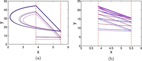
Let r = 1, k = 10, $\text{β}=0.025$, a = 0.188, n = 0.3, m = 0.03, h = 5.5, which means that $\underset{\_}{h}<h<x^{\ast }$ and $F\left(T\right)$ is well defined. According to Theorem 3.1, there exists an order-1 periodic solution $\left(X\right(t),Y(t\left)\right)$ for system (18(18) $\left\{\begin{array}{ll}\left.\begin{array}{l}\frac{\mathrm{d}x}{\mathrm{d}t}=rx\left(1-\frac{x}{k}\right)-\text{β}xy\\ \frac{\mathrm{d}y}{\mathrm{d}t}=y(\text{β}x-\alpha )\end{array}\right\},& x<h,\\ \left.\begin{array}{l}\mathrm{\Delta }x=-nx\left(t\right)\\ \mathrm{\Delta }y=-my\left(t\right)+\tau \end{array}\right\},& x=h.\end{array}\right.$(18) ). Take the uniform step size ${\mathrm{\Delta }}_{t_i}=0.05$. When $\tau =30$, the computation gives $\omega =10.348$, $Y\left(\omega \right)=14.8256$, $Y\left({\omega }^{+}\right)=44.3808$ and $N=\frac{\omega }{{\mathrm{\Delta }}_{t_i}}=207$. Following Equation (18(18) $\left\{\begin{array}{ll}\left.\begin{array}{l}\frac{\mathrm{d}x}{\mathrm{d}t}=rx\left(1-\frac{x}{k}\right)-\text{β}xy\\ \frac{\mathrm{d}y}{\mathrm{d}t}=y(\text{β}x-\alpha )\end{array}\right\},& x<h,\\ \left.\begin{array}{l}\mathrm{\Delta }x=-nx\left(t\right)\\ \mathrm{\Delta }y=-my\left(t\right)+\tau \end{array}\right\},& x=h.\end{array}\right.$(18) ), we have $|{\overline{\mu }}_1|=0.5223<1$. Therefore, the order-1 periodic solution is orbitally asymptotically stable(see Figure 8a). Let $\tau =7$. Then $\omega =4.84$, $Y\left(\omega \right)=15.7080$, $Y\left({\omega }^{+}\right)=22.2368$ and N = 97, and hence ${\overline{\mu }}_1=0.2222<1$, which can be seen from Figure 8(b) that the order-1 periodic solution is orbitally asymptotically stable.

Figure 8. The stability of order-1 periodic solution of system under the case that $\underset{\_}{h}<h<x^{\ast }$ and $F\left(T\right)$ is well defined, where r = 1, k = 10, $\text{β}=0.025$, a = 0.188, n = 0.3, m = 0.03, h = 5.5 and $\mathrm{\Delta }{t}_i=0.05$ such that $|{\overline{\mu }}_1|<1$: (a) $\tau =30$ such that $F\left(T\right)>0$; (b) $\tau =7$ such that $F\left(T\right)<0$.

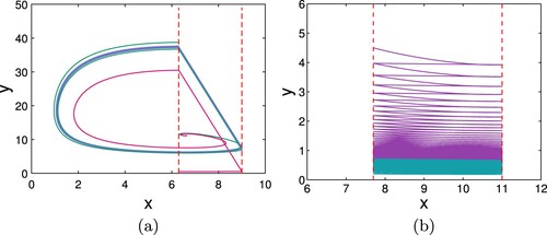
Fix r = 0.5, k = 15, $\text{β}=0.025$ and n = 0.3. Then $\underset{\_}{h}<x^{\ast }<h$. Let a = 0.165, m = 0.03, $\tau =30$, h = 9. Then $F\left(T\right)$ is not well defined, and $\omega =22.909$, $Y\left(\omega \right)=7.5269$, $Y\left({\omega }^{+}\right)=37.3011$. take $\mathrm{\Delta }{t}_i=0.25$. The calculation shows ${\overline{\mu }}_1=0.2956<1$. Further, let a = 0.27, m = 0, $\tau =0.05$, h = 11 and $\mathrm{\Delta }{t}_i=0.01$, the computation shows that $\omega =2.116$, $Y\left(\omega \right)=0.6663$, $Y\left({\omega }^{+}\right)=0.7163$ and N = 212, and hence $|{\overline{\mu }}_1|=0.9175<1$. Obviously, there is an orbitally asymptotically stable periodic solution of system, respectively, which can be seen from Figure 9(a) and Figure 9(b).

Figure 9. The stability of order-1 periodic solution of system when $\underset{\_}{h}<x^{\ast }<h$ and $F\left(T\right)$ is not well defined, where r = 0.5, k = 15, $\text{β}=0.025$ and n = 0.3 so that $|{\overline{\mu }}_1|<1$. (a) a = 0.165, m = 0.03, $\tau =30$, h = 9, and such that $I\left(R\right)>R^{-}$ and $P_N\left(R^{+}\right)>R^{-}$;(b) a = 0.27, m = 0, $\tau =0.05$, h = 11 and such that $I\left(R\right)<R_{-}$.

6. Conclusion and discussion

In the paper, the existence and existing domain, along with the stability of order-1 periodic solutions are considered. Further, we focus on the effects of parameters τ and m on the existence and stability of periodic solutions, which are performed theoretically and numerically. We construct three kinds of Bendixson domains with different structures, which overcome the difficulty, to some extent, that caused by the discontinuity of impulsive impact.

Our results show that the system (4(4) $\left\{\begin{array}{l}\frac{\mathrm{d}x}{\mathrm{d}t}=xU(x,y),\\ \frac{\mathrm{d}y}{\mathrm{d}t}=yV\left(x\right).\end{array}\right.$(4) ) without a positive periodic solution may have periodic oscillations under the effects of pulses. In this sense, the pulse action can ‘activate’ the state of periodic oscillation. When $h<x^{\ast }$, $F\left(T\right)$ must be well defined, and when $\underset{\_}{h}<x^{\ast }<h$, $F\left(T\right)$ is not necessarily well defined. If $F\left(T\right)$ is well defined, then system (2(2) $\left\{\begin{array}{ll}\left.\begin{array}{l}\frac{\mathrm{d}x}{\mathrm{d}t}=xU(x,y)\\ \frac{\mathrm{d}y}{\mathrm{d}t}=yV\left(x\right)\end{array}\right\},& x\ne h,\\ \left.\begin{array}{l}\mathrm{\Delta }x\left(t\right)=-nx\left(t\right)\\ \mathrm{\Delta }y\left(t\right)=-my\left(t\right)+\tau \end{array}\right\},& x=h,\end{array}\right.$(2) ) has an order-1 periodic solution, and when $\tau >0$, there must exist a positive order-1 periodic solution. If $F\left(T\right)$ is not well defined and the parameters τ and m are taken moderate values, the impulse effect will be invalid ultimately (see Theorem 3.4). If τ and $\frac{\tau }{m}$ are small enough, the population of the predator species, corresponding to y of the periodic solution, is also small. When $\frac{\tau }{m}$ is large enough, the periodic solutions locate in the sub-parallel domain (when $F\left(T\right)$ is well defined) or in the semi-ring domain (when $F\left(T\right)$ is not well defined), corresponding to a larger scale of predator species. When $\tau =0$, no matter $\underset{\_}{h}<h<x^{\ast }$ or $\underset{\_}{h}<x^{\ast }<h$ holds, there exist a semi-trivial periodic solution. However, when $\underset{\_}{h}<x^{\ast }<h$, there may still exist other positive order-1 periodic solutions (see Figure 7(a)).

From biological control point of view, when the density of the prey reaches a threshold h, the two species are harvested. When $\tau =0$, the system has a semi-trivial periodic solution, which means the predator becomes extinct, and the ecosystem is destroyed. Comparing Figure 4(c), Figure 5(c), Figure 7(b) with Figure 4(d), Figure 5(d), Figure 7(c), respectively, it can be seen that a small τ can ‘activate’ an positive order-1 periodic solution, which means the releasing of a small scale of predator can ‘stimulate’ an dynamic equilibrium of the ecosystem. When $|{\mu }_1|<1$, the dynamic equilibrium is stable, and we can implement the control of harvesting or releasing at every ω time, so as to maintain the ecological balance between the two species and to ensure the sustainable economic benefits.

Disclosure statement

No potential conflict of interest was reported by the author(s).

Additional information

Funding

This work was supported by The Natural Science Foundation of Hunan Province [2019JJ40240,2018JJ2319].

References

- D. Bainov and P. Simeonov, Impulsive Differential Equations: Periodic Solutions and Applications, Longman Scientific & Technical, England, 1993.
- E. Borducchi, C. Cabral, K. Stephenson, J. Liu, and H. Dan, Ad26/mva therapeutic vaccination with tlr7 stimulation in siv-infected rhesus monkeys, Nature 540 (2016), pp. 284–287.
- J. Chavez, D. Jungmann, and S. Siegmund, A comparative study of integrated pest management strategies based on impulsive control, J. Biological Dyn. 12 (2018), pp. 318–341.
- T. Cheng, S. Tang, and R.A. Cheke, Threshold dynamics and bifurcation of a state-dependent feedback nonlinear control SIR model, J. Comput. Nonlinear Dyn. 14 (2019), pp. 209.
- R. Hakl, M. Pinto, and V. Tkachenko, Almost periodic evolution systems with impulse action at state-dependent moments, J. Math. Anal. Appl. 446 (2017), pp. 1030–1045.
- Z. He, C. Li, L. Chen, and Zh. Cao, Dynamic behaviors of the FitzHugh–Nagumo neuron model with state-dependent impulsive effects, Neural Netw. 121 (2019), pp. 497–511.
- X. Hu, J. Li, and X. Feng, Threshold dynamics of a HCV model with virus to cell transmission in both liver with CTL immune response and the extrahepatic tissue, J. Biological Dyn. 15 (2021), pp. 19–34.
- G. Jiang, Q. Lu, and L. Qian, Complex dynamics of a Holling type II prey–predator system with state feedback control, Chaos Solit. Fract. 31 (2007), pp. 448–461.
- T. Kar and S. Chattopadhyay, A focus on long-run sustainability of a harvested prey predator system in the presence of alternative prey, Comp. Rend. Biol. 333 (2010), pp. 841–849.
- L. Li, Ch. Li, and W. Zhang, Existence of solution, pulse phenomena and stability criteria for state-dependent impulsive differential equations with saturation, Commun. Nonlinear Sci. Numer. Simul. 77 (2019), pp. 312–323.
- M. Liao, Y. Liu, Sh. Liu, and A. Meyad, Stability and Hopf bifurcation of HIV-1 model with Holling II infection rate and immune delay, J. Biological Dyn. (2021). Available at DOI:https://doi.org/10.1080/17513758.2021.1895334.
- L. Nie, J. Shen, and C. Yang, Dynamic behavior analysis of SIVS epidemic models with state-dependent pulse vaccination, Nonlinear Anal. Hybrid Syst. 27 (2018), pp. 258–270.
- L. Nie, Zh. Teng, H. Lin, and J. Peng, The dynamics of a Lotka-Volterra predator-prey model with state dependent impulsive harvest for predator, BioSystems 98 (2009), pp. 67–72.
- M. Nowak and R. May, Virus Dynamics: Mathematical Principles of Immunology and Virology, Oxford University Press, Oxford, 2000.
- P. Simeonov and D. Bainov, Orbital stability of periodic solutions of autonomous systems with impulse effect, Int. J. Syst. Sci.19 (1989), pp. 2561–2585.
- S. Tang and R. Cheke, State-dependent impulsive models of integrated pest management (IPM) strategies and their dynamic consequences, Math. Biol. 50 (2005), pp. 257–292.
- X. Tang and X. Fu, On period-k solution for a population system with state-dependent impulsive effect, J. Appl. Anal. Comput. 7 (2017), pp. 39–56.
- S. Tang, X. Tan, and J. Yang, Periodic solution bifurcation and spiking dynamics of impacting predator–prey dynamical model, Int. J. Bifurcation Chaos 28 (2018), pp. 1850147. Article ID 1850147.
- J. Wang, H. Chen, Y. Li, and X. Zhang, The geometrical analysis of a predator-prey model with multi-state dependent impulses, J. Appl. Anal. Comput. 8 (2018), pp. 427–442.
- H. Wang, B. Dai, and Q. Xiao, Existence of order-1 periodic solutions for a viral infection model with state-dependent impulsive control, Adv. Differ. Eq. 2019 (1) (2019). Available at https://doi.org/10.1186/s13662-019-1967-x.
- H. Wang, Ch. Ou, and B. Dai, The existence and stability of order-1 periodic solutions for an impulsive Kolmogorov predator–prey model with non-selective harvesting, J. Appl. Anal. Comput. 11(2021), pp. 1348–1370.
- A. Wang, Y. Xiao, and R. Smith, Using non-smooth models to determine thresholds for microbial pest management, J. Math. Biol. 78 (2019), pp. 1389–1424.
- Ch. Xu, M. Liao, P. Li, Y. Guo, Q. Xiao, and Sh. Yuan, Influence of multiple time delays on bifurcation of fractional-order neural networks, Appl. Math. Comput. 361 (2019), pp. 565–582.
- G. Zeng, L. Chen, and L. Sun, Existence of periodic solution of order one of planar impulsive autonomous system, J. Comput. Appl. Math. 186 (2006), pp. 466–481.
- Q. Zhang, B. Tang, and S. Tang, Vaccination threshold size and backward bifurcation of SIR model with state-dependent pulse control, J. Theoretical Biol. 455 (2018), pp. 75–85.
- Y. Zhou, Ch. Li, and H. Wang, Stability analysis on state-dependent impulsive hopfield neural networks via fixed-time impulsive comparison system method, Neurocomputing 316 (2018), pp. 20–29.