
 ?Mathematical formulae have been encoded as MathML and are displayed in this HTML version using MathJax in order to improve their display. Uncheck the box to turn MathJax off. This feature requires Javascript. Click on a formula to zoom.
Abstract
We propose two models inspired by the COVID-19 pandemic: a coupled disease-human behaviour (or disease-game theoretic), and a coupled disease-human behaviour-economic model, both of which account for the impact of social-distancing on disease control and economic growth. The models exhibit rich dynamical behaviour including multistable equilibria, a backward bifurcation, and sustained bounded periodic oscillations. Analyses of the first model suggests that the disease can be eliminated if everybody practices full social-distancing, but the most likely outcome is some level of disease coupled with some level of social-distancing. The same outcome is observed with the second model when the economy is weaker than the social norms to follow health directives. However, if the economy is stronger, it can support some level of social-distancing that can lead to disease elimination.
1. Introduction
Emerging infectious diseases, defined as new outbreaks triggered by unknown pathogens, or previously known infections which have spread to new geographic regions or whose incidence has increased dramatically within a geographic region in a short time have been on the rise within the past two decades [Citation6,Citation36,Citation41]. The pathogens that cause these infections can become efficiently human-to-human transmissible to generate large epidemics or pandemics. These epidemics or pandemics can have devastating public health and economic consequences to whole communities and countries, especially when there are limited or no immediate pharmaceutical mitigation and control measures at the time of emergence [Citation17,Citation24,Citation42]. An example of a pathogen that caused a global pandemic is SARS-CoV-2–the pathogen that is responsible for COVID-19. COVID-19 infected more than 107 million people, killed over 2.3 million people, and crippled the economies of many countries between late December 2020 and early February 2021 [Citation10,Citation24,Citation50].
The first line of defense against emerging influenza-like (respiratory) infections (which is generally aimed at slowing down the outbreak in order not to overwhelm healthcare systems or run down the economies of nations while pharmaceutical companies develop antiviral drugs and vaccines) are non-pharmaceutical interventions (NPIs) [Citation4,Citation8,Citation14,Citation21,Citation27,Citation28,Citation49]. These include quarantining of suspected cases, contact-tracing of the contacts of confirmed cases, isolation of confirmed cases, social-distancing, etc. Social-distancing entails limiting face-to-face contact with others in order to reduce disease spread [Citation5,Citation13,Citation16,Citation27]. In particular, social-distancing includes staying a certain distance (e.g. six feet in the case of COVID-19) apart in public, shelter-in-place mandates, partial or full lockdown of whole communities, businesses, schools, etc. These interventions are largely behavioural and from one side, if applied consistently and correctly can be instrumental for slowing down, and possibly stopping the outbreak, from another, they have the potential to cause significant hardship and economic loss. As observed with the COVID-19 pandemic, governments were faced with the trade-off between shutting down their economies (e.g. through strict large-scale shelter-in-place and lockdown mandates) in order to reduce the burden of the pandemic (e.g. the number of cases, hospitalizations, and deaths) and the stress on the healthcare systems or remaining open, i.e. easing these measures in order to save their economies from being paralyzed. Each option is associated with a positive and a negative outcome. For example, large-scale shelter-in-place and lockdowns will reduce the burden of the pandemic, but might drive the economy to depression. This will in turn reduce the amount of resources to be invested on healthcare. On the other hand, leaving the economy open will increase the burden of the pandemic, while increasing healthcare spending and reduced productivity associated with morbidity and mortality of members of the workforce. Nonetheless, the success of either option relies on human response to respect or not to respect the chosen measure. Human response whether to adopt a measure is determined by the risk associated with not adopting the measure and the payoff ensuing from adopting the measure. Thus, it is important to study the dynamics of these influenza-like diseases from a combined epidemiological, evolutionary game theory (or human-behavioural), and socio-economic perspective. Unfortunately, many infectious disease models fail to account for the joint contributions of these three components, let alone considering all three components in a single framework.
There has been significant interest in recent years in understanding the interaction between human behaviour and infectious diseases through multiple approaches including evolutionary game theory [Citation19]. In particular, Bauch [Citation1] and Poletti et al. [Citation39] have studied human behaviour change through imitation dynamics, while Breban [Citation3] used inductive games. Apart from a study by Reluga [Citation40] that used a game theory approach to investigate the impact of social-distancing on disease risk and another study by Ngonghala et al. [Citation26] that used a game theory approach in which human behaviour change is governed by three-state imitation dynamics to investigate the impact of social-isolation (e.g. self-quarantine and social-distancing) on the transmission dynamics and burden of COVID-19, the aforementioned approaches have been applied (1) mostly in the context of vaccination [Citation1,Citation18], (2) to understand the transmission dynamics of COVID-19 in Wuhan city of China [Citation52], (3) to assess the impact of the media on combating infectious diseases [Citation9], and (4) to assess the impact of human behaviour change and control measures to small pox [Citation45].
Coupled epidemiological-economic frameworks have been attracting attention within the scientific, public health, and economic communities. Specifically, coupled disease-economic models have been developed and used to assess feedbacks between disease and economic processes that can lead to vicious cycles of disease and poverty, as well as the impact of healthcare on breaking these vicious cycles [Citation2,Citation25,Citation29,Citation37,Citation38]. However, a single framework that accounts for the epidemiological component, evolutionary game theory component, i.e. the effects of human behavioural change in response to these diseases or control measures, and the economic component is missing from the literature.
Here, we develop a novel mathematical model framework (1) that is based on a coupled epidemiological-evolutionary game theory approach and use the framework to study the impact of human behaviour on the control of influenza-like illnesses, and (2) that incorporates an epidemiological, evolutionary game theory, and economic component and use the framework to study the interplay between human response to disease control measures, as well as the economic impact of diseases and human response to control measures. In both frameworks dynamic coupling of the separate components (i.e. the epidemiological, evolutionary game theory, and economic components) will be achieved through social-distancing. These novel models lead to new dynamics, new insights at the interface of disease-human behaviour-economics, and new conclusions. To our knowledge, this is the first study that couples models from three different areas (disease ecology, game theory, and economic growth) in a single framework and uses the framework to assess the impact of social-distancing in mitigating the epidemiological and economic burden of diseases.
In the next section we introduce a social-distancing coupled disease-human behaviour model which is inspired by the COVID-19 pandemic. We derive the model in the first subsection of the next section and analyse and simulate it in the second subsection. In the third subsection we consider the question of containing the disease when . In the first subsection of Section 3, we introduce a novel model at the interface of disease-human behaviour-economics, which we analyse and simulate in the second subsection (of this section). In the third subsection we address the problem of disease elimination when
in the context of social-distancing and economic growth. In the last section we discuss our results and present conclusions and limitations of the study.
2. A coupled disease-human behaviour model of social-distancing to control emerging diseases
Game theory is the study of mathematical (analytical) tools of strategic interaction among rational decision-makers. It has applications in many areas such as economics, philosophy and biology [Citation11,Citation32]. In the context of infectious diseases, evolutionary game theory has been applied mostly to study the impact of human behaviour or response to vaccination [Citation1,Citation51]. In this section we introduce a novel coupled disease-human behaviour model based on social-distancing. This is important because it can enhance our understanding of why some countries can eliminate a pandemic pathogen, while in other countries, the pathogen persists. Also, we develop the mathematical techniques, which will facilitate the study of evolutionary game theoretic models of social-distancing in general.
2.1. Deriving the coupled disease-human behaviour model of social-distancing
To link evolutionary game theory to social-distancing and hence disease dynamics, we assume that there are two strategies: Strategy A and Strategy B, where Strategy A involves keeping social-distancing strictly and contacting only family members in the same household, while Strategy B involves not respecting social-distancing strictly, i.e. contacting people who do not live in the same household. It should be mentioned that Strategy B includes both individuals who do not respect social-distancing at all, together with those who respect social-distancing but not in the strict sense. A possible extension of this work will be to split Strategy B into two separate strategies, i.e. those who do not respect social-distancing at all and those who do not respect social-distancing strictly. Let the proportion of individuals in the population, who adopt strategy A at time t, be and the proportion who adopt Strategy B at time t, be
. Then,
or
. In evolutionary game theory
and
are called replicators or players, who are producing their own strategies. As in [Citation18], the replicator equation is given by:
(1)
(1)
where the ‘
’ attached to
denotes differentiation with respect to time (t),
is the fitness of replicator i, and
is the average fitness in the system of replicators. With the replicator equation (Equation1
(1)
(1) ), the dynamics of the proportion of the population that is keeping social-distancing strictly is described by
As in [Citation1,Citation34], we assume that the fitness of keeping social-distancing strictly increases proportionally with the strength of social norms to follow health directives,
, weighted by the fraction of the population applying strategy A, and decreases by the cost,
, associated with applying strict social-distancing. That is, the fitness of replicator A is given by
. Similarly, the fitness of strategy B is given by
, where
is the fraction of individuals known to be infectious, and c is a proportionality constant. It should be mentioned that in this study, we are considering the case of strong selection, i.e. we are assuming that behaviour is completely determined by payoff/fitness, where the payoff matrix is given by:
To introduce a simple coupled disease-game theoretic model of social-distancing, we consider a generic susceptible-infectious-susceptible (SIS) model framework, with a constant human population. That is, we divide the total human population (which is assumed to be constant) into two mutually exclusive classes. Let
denote the number of susceptible individuals and
the number of infectious individuals in the population. Thus, the total circulating population at time t is
. We will denote by
and
the respective fractions of susceptible and infectious individuals, i.e.
and
, or
. Since we want to broaden the applicability of the framework, we incorporate vital dynamics, i.e. birth and death processes. We denote the daily recruitment rate by μ (all into the S class) and the daily natural death rate by μ. We assume that individuals recover at rate γ per day. The transmission rate for infectious individuals is β per day.
With the descriptions of the human behaviour and epidemiological models, the coupled disease-human behaviour model of social-distancing takes the following form:
(2)
(2)
where we have dropped the subscript A from x, i.e.
. The model is equipped with the initial conditions:
(3)
(3)
In system (Equation2
(2)
(2) ), we assume that social-distancing affects transmission and multiply the force of infection (
) by the proportion of individuals who practice only partial social-distancing or do not practice social-distancing at all,
. This is reasonable since social-distancing reduces the number of effective contacts, and hence the possibility of disease transmission.
2.2. Analytical and numerical results of Model (2)
Model (Equation2(2)
(2) ) is a simple framework with a unique infectious class, which appears to have relatively complex dynamics. The existence of equilibria depends on the parameters of the model, as well as the basic reproduction number of the disease system:
Considering the equilibria of the model (obtained by setting the left-hand sides of System (Equation2
(2)
(2) ) to zero and solving the resulting algebraic equations for the variables i and x), we have the following result:
Theorem 2.1
Model (Equation2(2)
(2) ) has five types of equilibria
| (1) | Disease-free, social-distancing free equilibrium | ||||
| (2) | Disease-free full social-distancing equilibrium | ||||
| (3) | Disease-free intermediate social-distancing | ||||
| (4) | A unique endemic equilibrium with no social-distancing | ||||
| (5) | One or more interior equilibria, e.g. | ||||
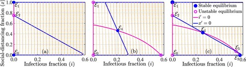
It should be noted that the trivial equilibrium represents the situation in which there is no disease and nobody is strictly social-distancing. Analytical results depicting the stability of the equilibrium points identified in Theorem 2.1 are presented in Theorem 2.2, while the number of equilibria and their stability are illustrated in Figure . For the parameter regime indicated in the caption of Figure , the disease-free social-distancing-free equilibrium
, is locally asymptotically stable since the disease reproduction number is
, the disease-free full social-distancing equilibrium
, is locally asymptotically stable since
, and the intermediate social-distancing equilibrium
is unstable (Figure (a)). In Figure (b), the unique interior equilibrium
, is locally asymptotically stable (or a spiral sink), while
,
, and
are unstable. Figure (c) shows that
is unstable (since
),
is locally asymptotically stable (since
), and
is locally asymptotically stable (since
). Also, the higher interior equilibrium
is locally asymptotically stable, while the lower interior equilibrium
and the intermediate social-distancing equilibrium
are unstable.
Figure 1. Phase plot of the coupled disease-game theory model (Equation2(2)
(2) ), illustrating various equilibria (i.e. the points of intersection of the blue and magenta curves denoted by filled blue and open magenta circles) for the parameter values (a)
per day and
per day, (b)
and
, and (c)
and
. The other parameter values used for the simulations are
per day,
per day,
per day and c = 1.
The presence of social-distancing in the population leads to a backward bifurcation of the interior equilibrium from a disease-free equilibrium with respect to the control reproduction number (Figure (c)–(d)). In such a case there are two interior equilibria for
(Figure (c)–(d)) and a unique interior equilibrium if
(red curves in Figure (a)–(b)). To derive the conditions for backward bifurcation, we consider the equations for the interior equilibria:
(4)
(4)
where we have divided both sides of the first equation by i, since i is non-zero at endemic or interior equilibria. From the second equation, we have
Since 0<x<1, we need i to satisfy
(5)
(5)
From the first equation, we have the following equation
(6)
(6)
The left-hand side of this equation is a parabola that opens down; the right-hand side is a horizontal line. If
, then the constant term in the i equation is negative, and the coefficient in front of i is positive, so there are 2 positive real solutions or no positive real solution by Descartes Rule of Signs. If
, then
is well-defined and two positive solutions exist if
through backward bifurcation (Figure (c)–(d)). Backward bifurcation with respect to
in this case occurs if and only if
. In both cases the two equilibria satisfy the condition
Then (Equation5
(5)
(5) ) is always satisfied if
and may or may not be satisfied if
.
Figure 2. Simulations of the coupled disease-game theory model (Equation2(2)
(2) ) depicting a forward bifurcation when
with
per day,
per day, c = 0.7 per day ((a) and (b)), and a backward bifurcation when
with
per day,
per day, c = 1.2 per day ((c) and (d)). The values of the other parameters used for the simulations are
per day and
per day. It should be mentioned that for these simulations, the disease transmission rate β is varied in the range
per day. The graphs illustrate typical stabilities of equilibria.
![Figure 2. Simulations of the coupled disease-game theory model (Equation2(2) i′=(1−x)βi(1−i)−(μ+γ)i,x′=x(1−x)(δ0x−rs+ci−δ0(1−x)),(2) ) depicting a forward bifurcation when δ0=rs+c with δ0=0.8 per day, rs=0.1 per day, c = 0.7 per day ((a) and (b)), and a backward bifurcation when δ0<rs+c with δ0=0.8 per day, rs=0.1 per day, c = 1.2 per day ((c) and (d)). The values of the other parameters used for the simulations are μ=0.01 per day and γ=0.4 per day. It should be mentioned that for these simulations, the disease transmission rate β is varied in the range [0,4] per day. The graphs illustrate typical stabilities of equilibria.](/cms/asset/cbead4bc-5216-4cd7-a098-7677e7528df8/tjbd_a_1946177_f0002_oc.jpg)
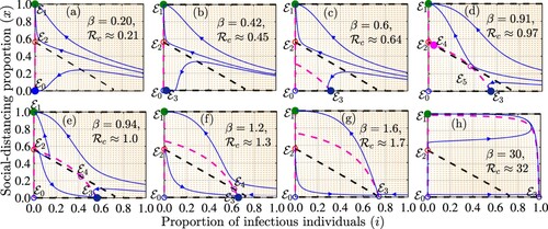
To better understand the emergence of the backward bifurcation, we simulated the model
(Equation2(2)
(2) ) when
for different values of the disease transmission rate (β). The results presented in Figure suggest that for a disease with low transmission, e.g. when
, both the disease-free social-distancing-free equilibrium (
) and the disease-free full social-distancing equilibrium (
) are locally asymptotically stable (Figure (a)). As the disease transmission rate increases (e.g. when
or
),
loses stability, while a stable infection social-distancing-free equilibrium (
) emerges Figure (b)–(c). Further increases in β (e.g. when
) lead to the emergence of two interior equilibria, one of which is locally asymptotically stable as long as the control reproduction number is less than unity (Figure (d)). Increasing β such that the control reproduction number is greater than or equal to one results to a scenario in which only
is stable as long as
.
Figure 3. Simulations of the coupled disease-game theory model (Equation2(2)
(2) ) depicting different equilibria (points of intersection of the dashed magenta and black curves denoted by filled blue and open magenta circles) and their stabilities for different values of the community transmission rate (β) and hence different control reproduction numbers (
). The dashed magenta and black curves are isoclines that correspond to the equations
and
, respectively. Sample solution trajectories are illustrated by blue curves. The values of the other parameters used for the simulations are
per day,
per day,
per day,
per day, and c = 1.2 per day. It should be mentioned that
for each graph.
Stability of equilibria to the model (Equation2(2)
(2) ) is somewhat unusual, particularly with regard to interior equilibria. In general, when a backward bifurcation occurs in epidemic models, the endemic equilibrium with a smaller proportion of infected individuals (i) is unstable, while the other endemic equilibrium with a larger proportion of infected individuals is stable [Citation23]. However, this is not the case here (Figure (c)). The replicator equation ‘switches’ the stability of interior equilibria and the interior endemic equilibrium with a smaller proportion of infected individuals is locally asymptotically stable or can lose stability through a Hopf bifurcation, while the other interior endemic equilibrium is unstable. We have the following Theorem concerning stability of equilibria:
Theorem 2.2
The equilibria of model (Equation2(2)
(2) ) have the following stabilities:
| (1) | The disease-free, social-distancing free equilibrium | ||||
| (2) | The disease-free full social-distancing equilibrium | ||||
| (3) | The disease-free intermediate social-distancing | ||||
| (4) | A unique no social-distancing endemic equilibrium | ||||
| (5) | The lower of the interior equilibria | ||||
Proof.
We prove 4 and 5. The Jacobian in its general form is given by
For the equilibrium
, we have
This equilibrium is locally asymptotically stable iff
or when
where
If
this equilibrium is unstable. Stability of
is given by the matrix
The characteristic equation corresponding to this Jacobian is given by
from where we obtain the following quadratic equation
The two interior equilibria differ by the sign of the slope at each equilibrium. Differentiating (Equation6
(6)
(6) ) we obtain that the lower equilibrium satisfies
The expression in the second parenthesis is 1−x, so we also have at the lower equilibrium
At the upper equilibrium, the opposite inequality holds:
Thus at the upper equilibrium we have for the constant term of the characteristic equation
Therefore, the characteristic equation at the upper equilibrium has a positive root and the upper equilibrium is always unstable. The constant term at the lower equilibrium is positive. Therefore, the lower equilibrium is locally asymptotically stable if
:
If
the equilibrium becomes unstable, with the stability lost through a Hopf bifurcation. The bifurcating periodic solution is stable (see Figure ).
Figure 4. Simulations of the model (Equation2(2)
(2) ) depicting the dynamics of the proportion of infectious individuals
as a function of time ((a) and (b)) and the proportion of individuals who are strictly socially-distancing
((c) and (d)) for different initial conditions. The dynamics for the first 50 days are illustrated in (a) and (c), while the remaining dynamics for days 50 to 250 are illustrated in (b) and (d). The parameter values used for the simulations are
per day,
per day,
per day,
per day,
per day, and c = 1.
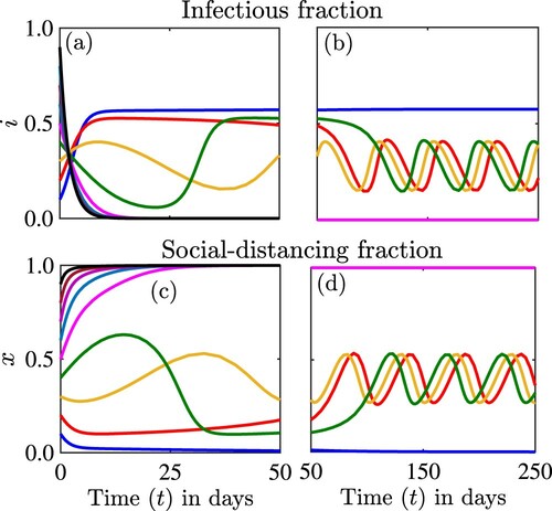
Figure shows that the solutions of the model can experience multiple stabilities. For this scenario two equilibria ,
, are locally asymptotically stable simultaneously. An interior equilibrium has lost stability through a Hopf bifurcation and we are observing sustained bounded periodic oscillations, which are also stable.
2.3. Can social-distancing lead to elimination of the disease?
Here, we address the question when . The short answer is – it depends; however, attaining and sustaining elimination with no strict social-distancing is not an option. This conclusion is supported by other authors including [Citation31]. If the social norms to follow health directives are stronger than the cost of strict social-distancing, that is
, then elimination is possible if all follow strict social-distancing. If the social norms to follow health directives are weaker than the cost of strict social-distancing, that is
, then elimination is not possible and the disease will persist at some level. The higher the proportion of the population following strict social-distancing, the lower the prevalence of the disease. The prevalence of the disease is highest if no one follows strict social-distancing. Because of the multi-stability, the end result also depends on the starting point. If the starting point has a high proportion following strict social-distancing, then the outcome is elimination of the disease; if the starting point has a low proportion of strictly socially distancing individuals, then the end result is disease persistence at a moderate or high level (Figure ).
3. A model at the disease-human behaviour-economic nexus
Now that we have a sound understanding of the interplay between social-distancing and disease, and that we have developed mathematical tools to study model (Equation2(2)
(2) ), we extend this knowledge to model the interplay between disease, social-distancing and economic growth. Hence, the next step towards modelling the complex disease-human behaviour-economic system is a coupled disease-human behaviour model of disease spread with an economic component. This study is inspired by the economic impact of COVID-19 and the measures taken to control the COVID-19 pandemic [Citation24,Citation30].
3.1. The disease-human behaviour-economic model
Mathematical models at the disease-economic nexus have been proposed and investigated in the literature, see, for example, [Citation25,Citation29]. Some of these models are based in part on the fact that socio-economic conditions are risk factors for infectious diseases [Citation22], while disease on the other hand can have a devastating impact on the economic status of individuals and communities. Many of these models have focused primarily on understanding feedbacks between poverty and ecological drivers of poverty such as infectious diseases and renewable resources in rural areas of resource challenged communities. However, the COVID-19 pandemic has demonstrated that infectious diseases may impact not only economically challenged rural communities, but also developed economies including world economic leaders [Citation10]. In particular, developed countries like the U.S., and many European countries bore the brunt of the burden of the COVID-19 pandemic, with containment or elimination prospects seemingly not dependent on the economic status of these countries [Citation10]. NPIs including border closures, quarantine of suspected COVID-19 cases, isolation of confirmed COVID-19 cases, and social-distancing, e.g. lockdown mandates implemented in an effort to fight the pandemic affected almost every economic sector of many countries around the world. Specifically, these measures slowed down economic activities in many countries through job losses, disruption of production, supply chains, consumption patterns, etc., [Citation24,Citation30,Citation33,Citation47]. School closures, for example, have a direct consequence on the accumulation of human capital (measured in terms of education or training of the workforce), which has the potential to influence future economic productivity [Citation25,Citation29]. Also, social-distancing, e.g. shelter-in-place and lockdown mandates, as well as COVID-related morbidities and mortalities impact economic productivity directly by reducing the workforce, especially in industries that require physical labour, e.g. agriculture. In the midst of this, the need for medical and personal protective equipment has been on the rise, while testing and managing COVID-19 infected cases require economic resources. This interdependence between disease and economic activities is not limited to COVID-19. Therefore, it is important to understand this interdependence, especially in the context of emerging respiratory infectious diseases and human response to NPIs against these diseases. The lack of economic perspective has been identified as a serious drawback of the multiple COVID-19 mathematical models that have emerged since the beginning of the pandemic [Citation46]. The question is so important that it has driven some preliminary studies with limited mathematical discussion [Citation12]. Our goal here is to develop mathematical model frameworks, as well as the mathematical techniques to study these types of frameworks (an aspect that has been hitherto omitted in some of the earlier models that considered coupled disease-economic dynamics), and then use the developed framework and tools to understand the interplay between infectious diseases, human response to disease control measures, and the associated economic impact.
We build our model on the basis of system (Equation2(2)
(2) ). To introduce the model, we first discuss the economic component. The economic model is based on the neoclassical (Solow-Swan) economic growth model [Citation43,Citation44], which emphasizes structural relationships between different factors of production such as capital (e.g. equipment, infrastructure, education, health, etc.), labour, and economic productivity. Specifically, the neoclassical growth model describes the change in capital with time according to the equation
(7)
(7)
where s is the capital accumulation rate per unit of time, σ is the capital depreciation rate, K is the stock of capital, Y is a production function or the total output obtained by combining various factors of production (e.g. capital and labour), sY is capital investment, i.e. the portion of the output that is reinvested into capital, and
is capital depreciation, i.e. the decline in the value of capital. It should be clarified that through a process called production, capital is converted into output Y, a proportion of this output cY, where 0<c<1 is consumed, while the rest, i.e.
is reinvested into capital. The fraction 1−c is commonly denoted by s. For simplicity, we use the Cobb-Douglas production function [Citation7]
(8)
(8)
where α is a the elasticity of the output with respect to the capital, A is the labour-augmenting technology, and L is the labour. It is commonly assumed that the inputs of the production function, e.g. capital, exhibit decreasing returns to scale (i.e. economic growth is accelerated for low input levels and falls in the long run as the inputs are increased) so that
[Citation20]. Unlike constant return to scale, where increases in inputs will trigger proportional increases in output, for decreasing (increasing) returns to scale increases in input will cause less than (more than) proportional increases in the output in the long run. Because of this decreasing returns to scale assumption, the investment curve intersects with the depreciation curve in the model (Equation7
(7)
(7) ) in the long run resulting in a single (non-trivial) stable equilibrium point given by
or
. It is also commonly assumed that labour and labour-augmented technology grow exponentially, i.e.
where the initial values
and
are given and n and g are the respective growth rates of labour and technological progress per unit of time.
Unlike the types of diseases considered in [Citation25,Citation29], where the economic status of an individual or a community has a strong impact on disease transmission and recovery from infection, transmission of, or recovery from diseases like COVID-19 do not necessarily depend on economic status. Hence, the main dynamic coupling between the types of diseases considered in this study, the behaviour model, and the economic model is through social-distancing. Specifically, the coupled disease-human behaviour (or disease-game theoretic) model is linked to the economic model through labour productivity in the production function, i.e. economic productivity and hence capital accumulation is a function of social-distancing. This is justified by the fact that social-distancing mandates reduction of the available labour force and hence economic productivity, especially in the context of the types of industries that require in-person or physical labour under consideration in this study. With the assumption that full social-distancing only reduces labour, the aggregated production function becomes
(9)
(9)
and equation (Equation7
(7)
(7) ) becomes
(10)
(10)
It should be mentioned that 1−x can also be regarded as the proportion of the population that is still able to work (regardless of social-distancing, or morbidity/mortality from disease). It should also be mentioned that in the context of this study, production refers to producing actual physical goods. This applies, for example, to agricultural workers (e.g. farmers and meat factory workers), grocery store workers, manufacturing industries, etc. This assumption will be relaxed in a later study to incorporate the service industry, where even individuals who respect social-distancing strictly can contribute to economic productivity and hence capital accumulation by working remotely. It is convenient to rescale the variables of the economic model in per capita terms by setting
and
. In this case, y and k are the respective per capita output and capital, i.e. the output and capital per effective worker (or effective unit of labour), since we are assuming that labour growth is proportional to the workforce. It should be noted that k can also be regarded as the capital intensity, i.e. the amount of available capital with reference to the other factors of production. This scaling simplifies Equation (Equation10
(10)
(10) ) to:
(11)
(11)
where
and n and g are assumed to be constant.
According to studies in [Citation35,Citation48], the wealthy are more likely to comply with social-distancing measures than the poor. It should be mentioned that many of the poor in developed countries such as the US double as essential workers in restaurants, the hospitality industry, retail stores, meat packaging industries, etc., who live from pay check to pay check. As observed during the COVID-19 period in the US, some low income earners who were pushed into earning unemployment benefits were reluctant to return to work because they earned more through unemployment benefits [Citation15]. This points to the fact that being wealthy, or providing capital or income facilitates social-distancing. Hence, we assume that increasing capital facilitates social-distancing at rate ρ. Putting together Equations (Equation2(2)
(2) ) and (Equation11
(11)
(11) ), we obtain the following coupled disease-human behaviour-economic model:
(12)
(12)
Under normal circumstances, disease and economic processes occur on different time scales, with the economic time scale as long as generations. However, in the case of a pandemic like COVID-19, economic changes as a function of disease can occur on a faster time scale than even the time scale of the disease.
3.2. Mathematical properties of the disease-human behaviour-economic model
In this section, we want to understand the dynamical behaviour of model (Equation12(12)
(12) ). For analytical tractability, we set
. With this value of α, the equilibria of the model (Equation12
(12)
(12) ) satisfy the following nonlinear system of algebraic equations:
(13)
(13)
In the case when x = 0, the second equation is trivially satisfied. From the first equation we have two possible equilibria i = 0 or
. From the last equation, we also have two possible equilibria:
Hence, there are four resulting equilibria:
,
,
and
. When x = 1, the second equation is again trivially satisfied. From the last equation we have k = 0. From the first equation, we have i = 0. The resulting equilibrium is
. Finally we consider the case 0<x<1. From the last equation we have either k = 0 or for interior equilibria we have
For k = 0, we have from the discussion in the previous section that there could be one or two equilibria of the form
. We also have a unique equilibrium of the form
. To find the interior equilibria, we use
and substitute into
(14)
(14)
Solving for x we have
Thus, this equilibrium exists iff
(15)
(15)
For the interior equilibria from the second equation and above we have
(16)
(16)
Expressing x in terms of i from the first equation, we get
In order for x>0 we need
(17)
(17)
Substituting in equation (Equation14
(14)
(14) ), we have
Simplifying, we have
(18)
(18)
The following results gives the existence of interior equilibria
Theorem 3.1
Assume .
| (1.) | If | ||||
| (2.) | If | ||||
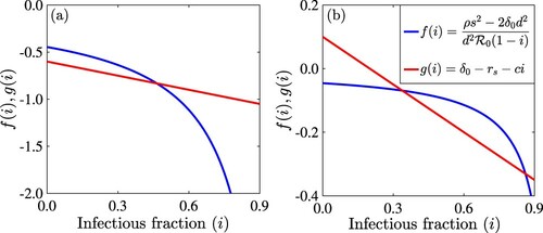
The possible number of interior equilibria from Theorem 3.1 are illustrated in Figure using the left- and right-hand sides of Equation (Equation18(18)
(18) ) (denoted by
and
). The model can have one interior equilibrium (Figure (a)) or two interior equilibria (Figure (b)).
Figure 5. Figure showing the intersection of the right-hand side (red line or ) and left-hand side (blue curve or
) of the equation (Equation18
(18)
(18) ) for (a)
and (b)
. The other parameter values used are
per day,
per day, s = 0.1 per day, d = 0.5 per day, c = 0.5, and q = 0.9. The value of the basic reproduction number is
.
To investigate the stability of the equilibria we compute the generic Jacobian.
For the stability of
we have
Thus, equilibrium
is always unstable. For the stability of
, we have
Thus equilibrium
is locally asymptotically stable if
and
, and unstable if
or
. The stability of equilibrium
is determined by the Jacobian:
Thus, equilibrium
is unstable if
. Because the last entry is undetermined, stability of this equilibrium in the case
cannot be determined from the Jacobian. The stability of equilibrium
is given by the Jacobian:
Thus, equilibrium
is locally asymptotically stable if
(19)
(19)
and unstable if
(20)
(20)
Just as the equilibrium
, the equilibrium
is always unstable. Next, we consider the stability of equilibria
. We have the following Jacobian for them.
Hence, equilibria
are unstable. The stability of
is given by
This equilibrium is stable if
(21)
(21)
The equilibrium is unstable if either inequality is reversed, that is, it is unstable if
(22)
(22)
The stability of interior equilibria is given by the generic Jacobian. We notice that at the interior equilibrium the generic Jacobian can be simplified as follows:
The characteristic equation is given by
We rewrite this as a cubic polynomial
where
From Equation (Equation18
(18)
(18) ) we see that the slopes at the lower equilibrium satisfy:
and the opposite inequality at the higher equilibrium. We can rewrite this inequality as
Thus, at the lower equilibrium, we have for the constant term
At the same time, at the upper equilibrium we have C<0 and we conclude that the upper equilibrium is unstable. At a unique equilibrium when
, we have
and therefore C<0 and such an equilibrium is unstable. At the unique equilibrium when
, we have
Hence, C>0 and such equilibrium has the potential to be stable but it may lose stability through a Hopf bifurcation. We summarize the results on the existence of equilibria and their local stability in Table .
Table 1. Existence and stability of equilibria.
3.3. Simulations of the disease-human behaviour-economic model
Table suggests that out of ten possible equilibria, only five have the potential to be locally stable. For the simulations, we consider the case , which leaves four equilibria as being possibly stable or losing stability to stable periodic orbits. Each of these equilibria can be reached through simulations. For example, Figure shows the stability of
where the disease persists without social-distancing and the economy is intact at equilibrium level. For the parameters in Figure we have
and
. Since
the stability of
is unclear from the analysis but the simulation suggests that
is stable.
Figure 6. Simulations of the model (Equation12(12)
(12) ) depicting the dynamics of the proportion of infectious individuals,
((a) and (d)), the proportion of individuals who are strictly social-distancing,
((b) and (e)), and the capital per effective worker,
((c) and (f)) as a function of time for different initial conditions. Dynamics for the first 20 days from (e)-(f) are illustrated in (a)–(c). The parameter values used for the simulations are
per day,
per day, c = 0.2,
per day,
per day,
per day,
per day, s = 0.1 per day, and d = 0.5 per day.
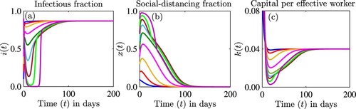
Figure shows the stability of the interior equilibrium. In this case the disease persists at a lower level, social-distancing is applied at about , and the economy is affected and persists at a lower level. In this case
, but
. We did not detect multi-stability in this case, although it is possible we did not explore all initial conditions. The simulations suggested that
may be unstable.
Figure 7. Simulations of the model (Equation12(12)
(12) ) showing the dynamics of (a) the proportion of infectious individuals
, (b) the proportion of individuals who are strictly social-distancing
, and (c) the capital per effective worker
as a function of time for different initial conditions. The parameter values used for the simulations are
per day,
per day, c = 0.4,
per day,
per day,
per day,
per day, s = 0.1 per day, d = 0.5 per day.
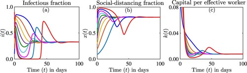
In Figure , we demonstrate several different concepts. First we show that the interior equilibrium can lose stability and that sustained oscillations are possible. Second, we show that multi-stability is possible in this model although it appears to be rare. As multi-stability occurs, we have two stable solutions – sustained oscillations around the interior equilibrium, and equilibrium . Third, we show that the equilibrium
may be stable, even though our analysis was inconclusive in this case.
Figure 8. Simulations of the model (Equation12(12)
(12) ) depicting the dynamics of the proportion of infectious individuals,
((a) and (d)), the proportion of individuals who are strictly social-distancing,
((b) and (e)), and the capital per effective worker,
((c) and (f)) as a function of time for different initial conditions. Dynamics for the first 20 days from (e)-(f) are illustrated in (a)–(c). The parameter values used for the simulations are
per day,
per day, c = 1,
per day,
per day,
per day,
per day, s = 0.1 per day, and d = 0.3 per day.

Figure is an extension of Figure to the disease-human behaviour-economic model. The reproduction number is . Compared to Figures and has only
stable. Thus, the presence of capital to be used in funding social-distancing makes the equilibrium
unstable and not attractive.
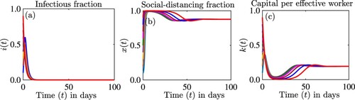
Figures – occur when . But, when
, the equilibrium
, can be stable and the disease can be eliminated with a high level of social-distancing maintained through capital infusions. We illustrate this in Figure . In this figure
, but we do not find bistability.
Figure 9. Simulations of the model (Equation12(12)
(12) ) showing the dynamics of (a) the proportion of infectious individuals
, (b) the proportion of individuals who are strictly social-distancing
, and (c) the capital per effective worker
as a function of time for different initial conditions. The parameter values used for the simulations are
per day,
per day, c = 2.7,
per day,
per day,
per day,
per day, s = 0.5 per day, d = 0.4 per day.
3.4. The disease-human behaviour-economic interplay
We address the question, ‘How does capital help with disease elimination when ?’ It turns out that elimination is possible both in the case when the economy is stronger than the social norms
and when it is weaker, i.e. when
. However, the long-term outlook for the economy is different and the proportion of individuals who engage in strict or full social-distancing is different. If the economy is weaker than the social norms, elimination of the disease is only possible when
of the population practices complete social-distancing. This leads to exhaustion and possible collapse of the economy. This scenario, although leading to disease-elimination is unlikely to be attainable or sustainable under realistic conditions. On the other hand, if the economy is stronger than the social norms, elimination of the disease is possible when only a potentially small fraction of the population practices complete social-distancing. This leads to, possibly, lower capital persistence but the economy does not collapse. This scenario leading to disease-elimination is attainable or sustainable under realistic conditions.
4. Discussion
This paper introduces two models: a coupled disease-human behaviour (or disease-game theoretic) model to study the impact of full social-distancing, and a coupled disease-human behaviour model with an economic component to study the interplay between infectious diseases, human behaviour, and economic growth. The first model can have five different kinds of equilibria: a disease-free social-distancing free equilibrium, which is stable if and unstable if
; a disease-free full social-distancing equilibrium, which is stable if social norms to follow health directives are stronger than the cost of full social-distancing, and unstable otherwise; a disease-free intermediate level of full social-distancing, which is always unstable; an endemic equilibrium without full social-distancing, which is stable if the replicator reproduction number is smaller than one, i.e.
and unstable otherwise; and one or two interior equilibria, one of which may be stable while the other is unstable. The stable interior equilibrium may lose stability via a Hopf bifurcation and sustained periodic oscillations are possible. When
, there are three possible outcomes: disease persistence without full social-distancing, disease persistence at a lower level of the fraction of the population practicing full social-distancing, and disease eradication with
of the population practicing full social-distancing.
Next, we introduced a model of social-distancing with an economic compartment. The second model has ten possible equilibria. These include an extinction equilibrium, with no disease, no strict social-distancing, and a possibility of the economy collapsing. This equilibrium is always unstable. There are three equilibria with only one non-trivial component: an equilibrium where the disease persists but there is no social-distancing and the economy collapses. This equilibrium is always unstable. There is also an equilibrium where everyone practices full social-distancing and there is no disease and the economy collapses. This equilibrium is always unstable. The third equilibrium occurs when there is no disease and no social-distancing, but the economy persists at its usual level. This equilibrium is stable under certain conditions. We also found another group of three equilibria in which one of the components is trivial, and the other two are non-trivial. The first of these three equilibria is an equilibrium in which there is no disease, but part of the population practices complete social-distancing and the economy is persisting at some level, another equilibrium when there is no complete social-distancing, the disease persists, and the economy is at some level. These two are stable under appropriate conditions. The last of these three equilibria is an equilibrium in which the disease persists, a portion of the population practices complete social-distancing, but the economy collapses. This equilibrium is unstable. The last equilibrium is the interior equilibrium. As in the first model the interior equilibrium can undergo backward bifurcation and multiple interior equilibria are possible. When multiple equilibria exist, the lower one (i.e. the one with a smaller proportion of infectious individuals) is locally stable, while the upper one (i.e. the one with a larger proportion of infectious individuals) is unstable. When a unique equilibrium exists it could be stable or unstable depending on additional conditions. A stable interior equilibrium can lose stability through a Hopf bifurcation accompanied by sustained oscillations.
We asked the question ‘When can the disease be eliminated in the case ?’. It turns out that disease elimination might be possible. According to the first model this is possible only if the entire population practices complete social-distancing. The second model, however, highlights the role of the economy. If the economy is weaker than the social norms, then elimination of the disease is only possible if the entire population practices complete social-distancing, a scenario that is potentially not very realistic. If however, the economy is stronger than the social norms, then elimination is possible with some portion of the population practicing complete social-distancing at the expense of the economy.
In both systems, we modelled disease transmission through a generic susceptible-infectious-susceptible (SIS) framework. Our goal in this manuscript was to understand the interplay between infectious diseases that can be controlled using NPIs such as social-distancing, human response to interventions against these diseases and economic growth from an analytical and numerical perspective. Hence, we used simplified models for analytical tractability. However, we used COVID-19 to motivate the study since it was ongoing at the time of the study and an intervention like social-distancing was instrumental in the fight against COVID-19. Although using a simple SIS model enabled us to be able to explore various properties and behaviours of the model analytically and numerically, it is restrictive and might not be applied directly to model COVID-19. An extension of the framework involving more realistic epidemiological features of COVID-19 such as pre-symptomatic infectious, asymptomatic infectious, hospitalized, and recovered classes, as well as COVID-19 related mortalities is currently under investigation. Another possible extension includes the role of testing and vaccines in the fight against the COVID-19 pandemic. It should also be mentioned that this study was performed with randomly selected parameter values since our goal was to illustrate the analytical results and to explore various dynamical behaviours. However, a future study will consider a more realistic framework in which disease, human behaviour, and economic data will be used to calibrate the parameters of the model. Another possible extension include considering economic processes that do not rely on the production of physical goods, where people can work remotely, while fully social-distancing. Furthermore, Strategy B can be broken into two other strategies involving individuals who do not adopt social-distancing at all and individuals who adopt social-distancing only partially.
Disclosure statement
No potential conflict of interest was reported by the author(s).
References
- C.T. Bauch, Imitation dynamics predict vaccinating behaviour, Proc. R. Soc. B: Biol. Sci. 272(1573) (2005), pp. 1669–1675.
- M.H. Bonds, D.C. Keenan, P. Rohani, and J.D. Sachs, Poverty trap formed by the ecology of infectious diseases, Proc. R. Soc. B: Biol. Sci. 277(1685) (2010), pp. 1185–1192.
- R. Breban, Health newscasts for increasing influenza vaccination coverage: An inductive reasoning game approach, PloS One 6(12) (2011), pp. e28300.
- Centers for Disease Control and Prevention, Nonpharmaceutical interventions (NPI), CDC Information, assessed on February 10, 2021.
- Centers for Disease Control and Prevention, Social distancing. Keep a safe distance to slow the spread, CDC Information, assessed on February 10, 2021.
- Centers for Disease Control and Prevention, Emerging infectious diseases, The National Institute for Occupational Safety and Health, assessed on January 18, 2021.
- C.W. Cobb and P.H. Douglas, A theory of production, Am. Econ. Rev. 18(1) (1928), pp. 139–165.
- B.J. Cowling, K.-H. Chan, V.J. Fang, C.K. Y Cheng, R.O. P Fung, W. Wai, J. Sin, W. Hong Seto, R. Yung, D.W.S. Chu, B.C.F. Chiu, P.W.Y. Lee, M.C. Chiu, H.C. Lee, T.M. Uyeki, P.M. Houck, J.S. Malik Peiris, and G.M. Leung, Facemasks and hand hygiene to prevent influenza transmission in households a cluster randomized trial, Ann. Inter. Med. 151(7) (2009), pp. 437–446.
- J. Cui, Y. Sun, and H. Zhu, The impact of media on the control of infectious diseases, J. Dyn. Differ. Equ. 20(1) (2008), pp. 31–53.
- E. Dong, H. Du and L. Gardner, An interactive web-based dashboard to track COVID-19 in real time, Lancet Infect. Dis. 20(5) (2020), pp. 533–534.
- R Gibbons, A Primer in Game Theory, Harvester Wheatsheaf, New York, 1992.
- U. Goldsztejn, D. Schwartzman, and A. Nehorai, Public policy and economic dynamics of COVID-19 spread: A mathematical modeling study, PloS One 15(12) (2020), pp. e0244174.
- M. Greenstone and V. Nigam, Does social distancing matter? University of Chicago, Becker Friedman Institute for Economics Working Paper, 2020.
- A.B. Gumel, E.A. Iboi, C.N. Ngonghala, and E.H. Elbasha, A primer on using mathematics to understand COVID-19 dynamics: Modeling, analysis and simulations, Infect. Dis. Model. 6 (2021), pp. 148–168.
- J. Kelly, Furloughed workers don't want to return to their jobs as they re earning more money with unemployment, Forbes, accessed on January 25, 2021
- J.A. Lewnard and N.C. Lo, Scientific and ethical basis for social-distancing interventions against COVID-19, Lancet Infect. Dis. 20(6) (2020), pp. 631–633.
- Q. Li, X. Guan, P. Wu, X. Wang, L. Zhou, Y. Tong, R. Ren, K.S. M Leung, E.H. Y Lau, J.Y. Wong, X. Xing, N. Xiang, Y. Wu, C. Li, Q. Chen, D. Li, T. Liu, J. Zhao, M. Liu, W. Tu, C. Chen, L. Jin, R. Yang, Q. Wang, S. Zhou, R. Wang, H. Liu, Y. Luo, Y. Liu, G. Shao, H. Li, Z. Tao, Y. Yang, Z. Deng, B. Liu, Z. Ma, Y. Zhang, G. Shi, T.T.Y. Lam, J.T. Wu, G.F. Gao, B.J. Cowling, B. Yang, G.M. Leung, and Z. Feng, Early transmission dynamics in Wuhan, China, of novel coronavirus-infected pneumonia, New England J. Med. 382 (2020), pp. 1199–1207.
- X.-Z. Li, J. Yang, and M. Martcheva, Age-structured epidemic models, in Age Structured Epidemic Modeling, X.-Z. Li, J. Yang, and M. Martcheva, eds., Springer, Cham, 2020, pp. 23–67.
- P. Manfredi and A. D'Onofrio, Modeling the Interplay Between Human Behavior and the Spread of Infectious Diseases, Springer Science & Business Media, New York, NY, 2013.
- N.G. Mankiw, D. Romer, and D.N. Weil, A contribution to the empirics of economic growth, Quart. J. Econ. 107(2) (1992), pp. 407–437.
- H. Markel, H.B. Lipman, J.A. Navarro, A. Sloan, J.R. Michalsen, A.M. Stern, and M.S. Cetron, Nonpharmaceutical interventions implemented by us cities during the 1918–1919 influenza pandemic, J. Am. Med. Assoc. 298(6) (2007), pp. 644–654.
- M. Marmot, Social determinants of health inequalities, Lancet 365(9464) (2005), pp. 1099–1104.
- M. Martcheva, Methods for deriving necessary and sufficient conditions for backward bifurcation, J. Biol. Dyn. 13(1) (2019), pp. 538–566.
- W. McKibbin and R. Fernando, The economic impact of COVID-19, Econ. Time COVID-19 45 (2020), pp. 45–51.
- C.N. Ngonghala, G.A. De Leo, M.M. Pascual, D.C. Keenan, A.P. Dobson, and M.H. Bonds, General ecological models for human subsistence, health and poverty, Nat. Ecol. Evol. 1(8) (2017), pp. 1153–1159.
- C.N. Ngonghala, P. Goel, D. Kutor, and S. Bhattacharyya, Human choice to self-isolate in the face of the COVID-19 pandemic: A game dynamic modelling approach, J. Theor. Biol. 521 (2021), pp. 110692.
- C.N. Ngonghala, E. Iboi, S. Eikenberry, M. Scotch, C.R. MacIntyre, M.H. Bonds, and Abba B Gumel, Mathematical assessment of the impact of non-pharmaceutical interventions on curtailing the 2019 novel coronavirus, Math. Biosci. 325 (2020), p. 108364.
- C.N. Ngonghala, E.A. Iboi, and A.B. Gumel, Could masks curtail the post-lockdown resurgence of COVID-19 in the US? Math. Biosci. 329 (2020), p. 108452.
- C.N. Ngonghala, M.M. Pluciński, M.B. Murray, P.E. Farmer, C.B. Barrett, D.C. Keenan, and M.H. Bonds, Poverty, disease, and the ecology of complex systems, PLoS Biol. 12(4) (2014), p. e1001827.
- M. Nicola, Z. Alsafi, C. Sohrabi, A. Kerwan, A. A-Jabir, C. Iosifidis, M. Agha, and R. Agha, The socio-economic implications of the coronavirus and COVID-19 pandemic: A review, Inter. J. Surg. 78 (2020), pp. 185–193.
- J.Y. Noh, H. Seong, J.G. Yoon, J.Y. Song, H.J. Cheong, and W.J. Kim, Social distancing against COVID-19: Implication for the control of influenza, J. Korean Med. Sci. 35(19) (2020), pp. e182.
- M.J. Osborne and A. Rubinstein, A Course in Game Theory, MIT Press, Cambridge, MA, 1994.
- P.K. Ozili and T. Arun, Spillover of COVID-19: Impact on the global economy, available at SSRN 3562570, 2020.
- A.D. Pananos, T.M. Bury, C. Wang, J. Schonfeld, S.P. Mohanty, B. Nyhan, M. Salathé, and C.T. Bauch, Critical dynamics in population vaccinating behavior, Proc. Natl. Acad. Sci. 114(52) (2017), pp. 13762–13767.
- N.W. Papageorge, M.V. Zahn, M. Belot, E. Van den Broek-Altenburg, S. Choi, J.C. Jamison, and E. Tripodi, Socio-demographic factors associated with self-protecting behavior during the COVID-19 pandemic, J. Popul. Econ. 34 (2020), pp. 691–738.
- J.A. Patz, P.R. Epstein, T.A. Burke, and J.M. Balbus, Global climate change and emerging infectious diseases, J. Am. Med. Assoc. 275(3) (1996), pp. 217–223.
- M.M. Pluciński, C.N. Ngonghala, and M.H. Bonds, Health safety nets can break cycles of poverty and disease: A stochastic ecological model, J. R. Soc. Interface 8(65) (2011), pp. 1796–1803.
- M.M. Pluciński, C.N. Ngonghala, W.M. Getz, and M.H. Bonds, Clusters of poverty and disease emerge from feedbacks on an epidemiological network, J. R. Soc. Interface 10(80) (2013), p. 20120656.
- P. Poletti, B. Caprile, M. Ajelli, A. Pugliese, and S. Merler, Spontaneous behavioural changes in response to epidemics, J. Theor. Biol. 260(1) (2009), pp. 31–40.
- T.C. Reluga, Game theory of social distancing in response to an epidemic, PLoS Comput. Biol. 6(5) (2010), p. e1000793.
- K.F. Smith, M. Goldberg, S. Rosenthal, L. Carlson, J. Chen, C. Chen, and S. Ramachandran, Global rise in human infectious disease outbreaks, J. R. Soc. Interface 11(101) (2014), p. 20140950.
- K.M. Smith, C.C. Machalaba, R. Seifman, Y. Feferholtz, and W.B. Karesh, Infectious disease and economics: The case for considering multi-sectoral impacts, One Health 7 (2019), p. 100080.
- R.M. Solow, A contribution to the theory of economic growth, Quart. J. Econ. 70(1) (1956), pp. 65–94.
- T.W. Swan, Economic growth and capital accumulation, Econ. Rec. 32(2) (1956), pp. 334–361.
- S.D. Valle, H. Hethcote, J.M. Hyman, and C. Castillo-Chavez, Effects of behavioral changes in a smallpox attack model, Math. Biosci. 195(2) (2005), pp. 228–251.
- J. Wang, Mathematical models for COVID-19: Applications, limitations, and potentials, J. Public Health Emer. 4 (2020), pp. 1–4.
- Q. Wang and M. Su, A preliminary assessment of the impact of COVID-19 on environment – a case study of China, Sci. Total Environ. 728 (2020), pp. 138915.
- J.A. Weill, M. Stigler, O. Deschenes, and M.R. Springborn, Social distancing responses to COVID-19 emergency declarations strongly differentiated by income, Proc. Natl. Acad. Sci. 117(33) (2020), pp. 19658–19660.
- World Health Organization Writing Group, Nonpharmaceutical interventions for pandemic influenza, national and community measures, Emerg. Infect. Dis. 12(1) (2006), p. 88.
- Worldometers, Coronavirus, Worldometers, assessed on February 10, 2020.
- J. Yang, M. Martcheva, and Y. Chen, Imitation dynamics of vaccine decision-making behaviours based on the game theory, J. Biol. Dyn. 10(1) (2016), pp. 31–58.
- S. Zhao, L. Stone, D. Gao, S.S. Musa, M.K. Chong, D. He, and M.H. Wang, Imitation dynamics in the mitigation of the novel coronavirus disease (COVID-19) outbreak in Wuhan, China from 2019 to 2020, Ann. Transl. Med. 8(7) (2020), pp. 448–462.