
 ?Mathematical formulae have been encoded as MathML and are displayed in this HTML version using MathJax in order to improve their display. Uncheck the box to turn MathJax off. This feature requires Javascript. Click on a formula to zoom.
Abstract
We study a population model where cells in one part of the cell cycle may affect the progress of cells in another part. If the influence, or feedback, from one part to another is negative, simulations of the model almost always result in multiple temporal clusters formed by groups of cells. We study regions in parameter space where periodic ‘k-cyclic’ solutions are stable. The regions of stability coincide with sub-triangles on which certain events occur in a fixed order. For boundary sub-triangles with order ‘’, we prove that the k-cyclic periodic solution is asymptotically stable if the index of the sub-triangle is relatively prime with respect to the number of clusters k and neutrally stable otherwise. For negative linear feedback, we prove that the interior of the parameter set is covered by stable sub-triangles, i.e. a stable k-cyclic solution always exists for some k. We observe numerically that the result also holds for many forms of nonlinear feedback, but may break down in extreme cases.
1. Introduction
1.1. Background
In biology, there are phenomena that may emerge when cells or other dynamical units are coupled and influence each other. One example is synchronization, a state in which units are progressing with identical or nearly identical coordinates. In this manuscript, we consider a related phenomenon, phase synchronization or temporal clustering, in which multiple groups (or clusters) of cells are synchronized. They have the same phase as the other cells in their group, but the phase differs from one group to another. Throughout this manuscript, ‘clustering’ will mean temporal clustering (not spatial clustering).
There is a huge literature about synchronization, but temporal clustering has been studied much less often. It was observed in models of connected neurons [Citation1,Citation14,Citation15,Citation20,Citation38] and models of coupled engineered biological oscillators [Citation11,Citation40]. Temporal clustering has been observed in some experiments, including coupled chemical oscillators based on the Belousov–Zhabotinski reaction [Citation34,Citation35] and engineered electrochemical arrays [Citation16,Citation17,Citation37].
Temporal clustering also has been observed in Yeast Metabolic Oscillations (YMO) experiments that exhibit stable periodic oscillations of budding yeast (Saccharomyces cerevisiae) between aerobic metabolism and anaerobic metabolism. These have been observed in experiments and studied for many years [Citation8,Citation12,Citation19,Citation21,Citation27,Citation31].
The Cell Division Cycle (CDC) of budding yeast is the cyclic process of cell growth and division. A correlation between YMO and bud index, fraction of cells budded, was presented very early [Citation19,Citation21], but the link between YMO and the CDC was unclear due to the fact that the periods of YMO were always shorter than the CDC times in the same experiments. The relationship between YMO and the CDC was mostly ignored until it was noted in genetic expression data [Citation18,Citation31] and investigators began calling such oscillations ‘cell cycle related’. Boczko et al. [Citation3] proposed that temporal clustering is the mechanism linking the metabolism and the CDC in these experiments. Temporal clustering with two clusters was observed in YMO experiments reported in Stowers et al. [Citation33] and Young et al. [Citation39] and it was postulated that cells are segregated into CDC synchronized clusters due to feedback effects on the CDC progression. They proposed that cells in some phase of the cell cycle might produce signalling agents or metabolic products and the levels of these chemicals may affect the growth rate of cells in some other parts of the cycle.
Population level models of the cell cycle that include the effect of such feedback between different parts of the cell cycle were proposed in Boczko et al. [Citation3] and Young et al. [Citation39]. It was observed in [Citation5] that clustering in these models is heavily related to a number theoretic relationship between the number of clusters k and other indices that characterize possible clustered solutions. The main goal of this manuscript is to prove a conjecture made in [Citation5] that for negative feedback, temporal clustering is universal, meaning that it happens for any parameters in the model.
1.2. A cell cycle population model, notations and previous results
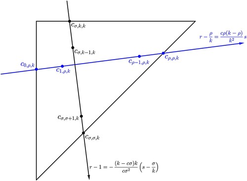
We will represent the progress of a cell by a variable (phase) ; 0 is the beginning of the cell division cycle and 1 is the end of the cycle. We will identify 0 with 1 and consider
as a normalized coordinate on the circle. We will let
and
where 0<s<r<1; see Figure . The model of progress of the ith cell in the cell cycle conceptualized in [Citation3] is as follows:
(1)
(1) where
,
(2)
(2) We will assume that f is a monotone function satisfying
and
. It is perhaps nonlinear.
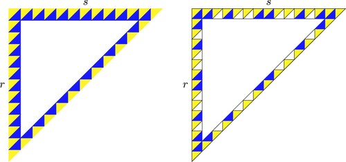
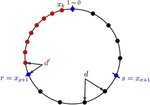
Figure 1. Schematic with 11 cells where 3 cells are in the S region and 7 cells are in (outside the R region). According to the model,
to
are progressing with rate 1 while
to
are progressing with rate
.
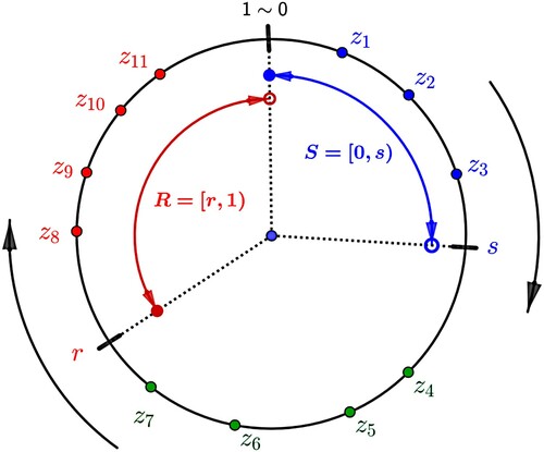
The key feature of the model is that cells in one part of the cycle (denoted by for signalling) influence the cells in another part (
for responsive). We postulate that the feedback is not direct from cell to cell, but is exerted through the influence of chemicals in the medium that are produced or perhaps consumed by cells in different regions of the cycle. The numbers 0<s<r<1 are fixed for a given application. We will treat them as parameters of the dynamical system. Previous work [Citation39] shows that the number of clusters in asymptotically stable solutions is strongly dependent on s and r.
We do not know how the coordinates of our model correspond to particular phases of the actual cell cycle and so it does not reflect specific biology. However, it is well established that different parts of the cell cycle produce, consume and react differently to different metabolites and other chemicals (see, e.g. [Citation7,Citation9,Citation13,Citation24–26,Citation36,Citation41]). A checkpoint, a phase of the cell cycle where progress may be arrested until sufficient conditions are satisfied [Citation13], is a natural candidate for a responsive phase (R in our model) with negative feedback. This particular mechanism was modelled and studied in [Citation22].
We note that the right-hand side of the differential equation (Equation1(1)
(1) ) is piecewise constant. Solutions fail to be differentiable at discrete points in time, and the definition of solution must be generalized to continuous, piece-wise smooth solutions. This was addressed in [Citation39].
Figure provides a visualization of the system in model (Equation1(1)
(1) ) for the case of n = 11 where 11 different locations of cells represent the state of each cell in the cycle.
Note that cells are identical in (Equation1(1)
(1) ) and so if two cells have the same coordinates at some time
, then they will coincide for all
. A cluster will mean a group of cells whose coordinates are equal and the integer k will be the number of clusters.
When the cells are grouped in k clusters it is sufficient to consider only the k coordinates, of the clusters rather than the coordinates of all individual cells. It follows trivially that the progress of clusters is given by
(3)
(3) for
, and I is again given by (Equation2
(2)
(2) ). If the k clusters all have the same number of cells, then the progress of evenly clustered solutions can be described by (Equation3
(3)
(3) ), with
(4)
(4) the fraction of clusters in the signalling region.
Next, we define a special class of periodic, evenly clustered solutions of the system (Equation3(3)
(3) )–(Equation4
(4)
(4) ) that will be the main object of our study.
Definition 1.1
Let n be the total number of cells in the cycle and be a divisor of n, with n/k cells in each cluster. Suppose that there exists a smallest positive number d such that
for all
and
. Then
is called a k-cyclic solution.
The existence of k-cyclic solutions was proved in [Citation6,Citation39]: For any and any pair
, if k is a divisor of n, then a k-cyclic solution exists consisting of n/k cells in each cluster. For negative f and a given pair
, the k-cyclic solution is unique, up to a translation in time.
The main result of this manuscript is that for negative linear feedback, given any pair of parameters , 0<s<r<1, there is a
such that the unique k-cyclic solution corresponding to
is (locally) asymptotically stable. In order to prove this result, we will first establish new results about stability of k-cyclic solutions for
in certain subsets. This will require the introduction of quite a bit of terminology.
Let denote the initial condition of
and let
. For a solution with an initial condition in
, let
be the shortest positive time required for
to return back to its starting position, 0; i.e. when the solution returns to
. The Poincaré map
for the flow (Equation3
(3)
(3) )-(Equation4
(4)
(4) ) is defined as follows:
(5)
(5) Because we have assumed that
, this Poincaré map is well defined.
Definition 1.2
We define a map F by
(6)
(6) where
is the shortest time required for
to reach 1.
It was noted that the map is conjugate to the Poincaré map Π [Citation39]. Further, if
is a fixed point of F, then
is the initial condition of a k-cyclic solution of (Equation3
(3)
(3) )–(Equation4
(4)
(4) ) and vice versa. Moses [Citation23] showed that for k even clusters, asymptotic stability in the k clustered phase space implies asymptotic stability in the full phase space of n cells, i.e. system (Equation1
(1)
(1) )–(Equation2
(2)
(2) ). Thus, to study the stability of any k-cyclic solution, it is sufficient to study the stability of the fixed points of F.
Note that can be considered as a (closed) simplex. The map F is defined on the interior of the simplex, i.e. on
. It was shown in [Citation39] that the map F can be extended continuously to the boundary of the simplex and that this continuously extended F permutes components of the boundary of the simplex.
Define σ to be the number of clusters in at the initial time and define ρ to be the number of clusters in
(outside of R) at the initial time. That is,
(7)
(7) According to Equations (Equation3
(3)
(3) )–(Equation4
(4)
(4) ), clusters may change their rate only when one of them reaches
or 1 which we call events s, r and 1, respectively.
Definition 1.3
Let be a solution whose initial condition satisfies (Equation7
(7)
(7) ). Then,
reaching s is called the event
,
reaching r is called the event
,
reaching 1 is called the event
. A sequence
means that the clusters progress with an order of events
,
and
, respectively. If two or three events happen at the same time, we say that the solution has simultaneous events.
The sequence of events followed by a cyclic solution is periodic and either or
or has simultaneous events [Citation5]. Thus, if we wish to study the stability of cyclic solutions, we need only to consider two periodic sequences of events,
or
.
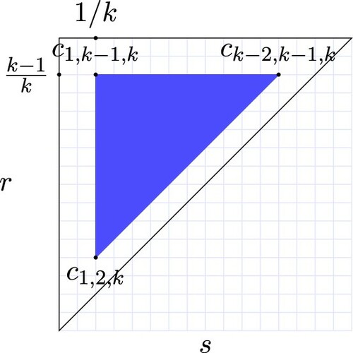
We will call the set of points the parameter triangle
.
Definition 1.4
A subset is called isosequential for k if the k-cyclic solution corresponding to each parameter pair in the interior of τ has the same σ and ρ and the same order of events:
,
That is, and
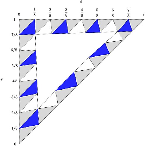
are regions on which the k-cyclic solutions have the order of events sr1 or rs1, respectively. Figure shows indices of isosequential regions for the case of k = 3. Isosequential regions are in fact sub-triangles [Citation5]. Figure illustrates that the relative positions of the parameters and the clusters of the cyclic solution determine the order of events.
Figure 2. Illustration of how sub-triangles are indexed for the case of k = 3 (and feedback function ). Each square corresponds to a pair
. Within squares, upper-left triangles
have cyclic solutions with the order of events
, while lower-right triangles
have the order of events
.
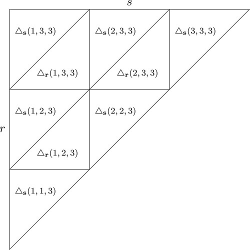
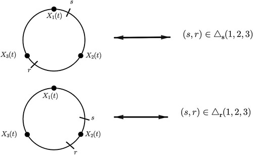
Figure 3. Top: will reach s before
reaches r, so the pair
. Bottom:
will reach r before
reaches s, so
.
Isosequential regions are important because it was shown in [Citation5] that all the k-cyclic solutions for in one of these sub-triangles have the same stability type. We will call a sub-triangle stable if all the k-cyclic solutions corresponding to points in the region are asymptotically stable. An isosequential region will be called unstable if all the k-cyclic solutions corresponding to points in the region are unstable. An isosequential region is called neutral if all the k-cyclic solutions corresponding to points in the region are neutrally stable (stable, but not asymptotically stable). In the context of k-cyclic solutions, stable means that initial conditions near the orbit of the periodic solution will remain near the orbit for all forward time. Asymptotic stability means that nearby solutions not only remain in a neighbourhood of the periodic orbit but also converge to the periodic orbit in forward time.
A point is called a simultaneous point if the k-cyclic solution has events
,
and
occurring simultaneously. Note that if
is a simultaneous point, then the initial condition (assumed to be in
) of the k-cyclic solution has one cluster located at s and another one at r. For any f and integer
isosequential regions are sub-triangles with simultaneous points at their corners [Citation5]. In the interior of each sub-triangle, all k-cyclic solutions have the same order of events and same stability.
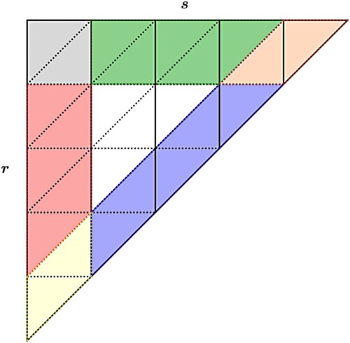
We define the following:
all the rest are called interior sub-triangles.
Figure 4. Boundary sub-triangles for the case of k = 5 and . The red sub-triangles are called vertical sub-triangles. The green sub-triangles are the horizontal sub-triangles. The purple sub-triangles are the oblique sub-triangles. The grey, yellow and orange sub-triangles are on two of the boundaries. The white sub-triangles are called interior sub-triangles.
Next we review previous results about the stability of cyclic solutions.
The vertical and horizontal boundary sub-triangles with order of events sr1, i.e. and
, were shown to be neutral for any
in [Citation5].
For horizontal and vertical sub-triangles with order , if
or
, respectively, the sub-triangle is stable for negative feedback. If
or
, then the sub-triangle is neutral.
For positive feedback, all interior sub-triangles are unstable and for negative feedback all interior sub-triangles with the order sr1 are unstable [Citation2,Citation23].
In conclusion, stability under negative and positive feedbacks of the vertical and horizontal sub-triangles was fully investigated in earlier works. However, stability of the oblique sub-triangles has not been previously analysed. The oblique sub-triangles are indexed by and
where
. All results that had been established previously are shown in Figure for the case of k = 8 where stability of the white sub-triangles has not been investigated before. In this manuscript, we prove that the stability of the oblique triangles follows a similar pattern as the vertical and horizontal sub-triangles.
Figure 5. An illustration of known results for k = 8. The grey regions are neutrally stable by results in [Citation5]. The left panel corresponds to a positive feedback: the red sub-triangles were shown to be unstable in [Citation2,Citation23], the green regions are unstable for large feedback [Citation23]. We will show that they are neutral for small feedback. The right panel corresponds to a negative feedback: the blue regions were shown to be asymptotically stable and the yellow areas neutrally stable in [Citation23], the red regions are unstable [Citation2].
![Figure 5. An illustration of known results for k = 8. The grey regions are neutrally stable by results in [Citation5]. The left panel corresponds to a positive feedback: the red sub-triangles were shown to be unstable in [Citation2,Citation23], the green regions are unstable for large feedback [Citation23]. We will show that they are neutral for small feedback. The right panel corresponds to a negative feedback: the blue regions were shown to be asymptotically stable and the yellow areas neutrally stable in [Citation23], the red regions are unstable [Citation2].](/cms/asset/43657521-15ef-45f1-8f81-5a1dfd39e7c4/tjbd_a_1971781_f0005_oc.jpg)
1.3. Main results
As discussed above, the stability of the vertical and horizontal sub-triangles was completely investigated, but the stability of the oblique sub-triangles was open. The ideas presented in Section 3 complete the study of stability of boundary sub-triangles. The stable sub-triangles are those with order of events rs1 and whose index is relatively prime with respect to the number of clusters k. Results in Section 3 can be combined into the following which was conjectured in [Citation5].
Theorem A
Consider the system (Equation3(3)
(3) )–(Equation2
(2)
(2) ) with any negative, non-increasing, feedback function
. For
, all triangles with edges on the boundary (order
) of
are neutral. Boundary triangles with order of events
are either neutral or stable. If we number them by an index i,
then a sub-triangle is stable if k and i are relatively prime and neutral otherwise.
This result is illustrated in Figure for k = 8. The grey (sr1) and white (rs1) areas in Figure are neutral. The blue shaded areas (rs1) in Figure are stable.
Figure 6. The boundary sub-triangles for the case of k = 8 under a negative feedback function. The blue sub-triangles rs1 are stable. The white rs1 and gray sr1 sub-triangles are neutral.
Our method not only clarifies the stability of oblique sub-triangles but also provides an alternative proof for the vertical and horizontal sub-triangles. We establish these results by analysing all eigenvalues of the Jacobian matrix of the map F corresponding to points in each isosequential region.
In Section 5, we prove our main result, which is the following.
Theorem B
For any negative linear feedback , c<1, and any pair
in the interior of the triangle 0<s<r<1, there is a positive integer k,
, such that the k-cyclic solution corresponding to
is stable.
This result is important because it means that negative linear feedback systems of this type will always possess an asymptotically stable clustered periodic solution, irrespective of the values of parameters.
This was conjectured more generally in [Citation5]. Numerically, this result appears to hold also for non-linear negative feedback, except possibly for some extreme cases. (See the last section for discussion.)
In Section 4. we prove a version of Theorem thmB in the case of the zero feedback limit where the main ideas are more clear.
These results appeared in expanded form in the dissertation of the first author [Citation28].
2. Some preliminaries
We introduce the following notations that will be used for the rest of this manuscript.
Note that for negative feedback,
.
2.1. Order of events rs1
Suppose that and let
be a solution of (Equation3
(3)
(3) )–(Equation4
(4)
(4) ) such that its initial condition (where
) satisfies (Equation7
(7)
(7) ) and
(8)
(8) This condition implies that the solution has order of events rs1.
Recall that as defined in (Equation6
(6)
(6) ). Formulas for F and its derivative DF were calculated in [Citation2]. Specifically,
is defined by the following.
The determinant of
was calculated to be
which is less than one in absolute value since
. For
, eigenvalues of
for sub-triangles
satisfy the equation
(9)
(9) and 1 is not an eigenvalue [Citation2].
2.2. Order of events sr1
Consider a k-clustered solution with order of events sr1. Then, its initial condition satisfies
(10)
(10) At the time
, [Citation2] obtained the solution
This defines the map
. The Jacobian matrix of the map DF for the order of events sr1 was shown in [Citation2] to be the following:
We note that this implies that k cyclic solutions with order
cannot be asymptotically stable. For
, eigenvalues of
for sub-triangles
satisfy the equation
(11)
(11) and 1 is not an eigenvalue [Citation2].
Recall that for a complex number, z = x + iy, an argument of z, , is a number
such that
and
, where
. Figure shows the general picture of
,
, and
for given
. The argument of
is the angle between the line from z to
and the horizontal line passing
.
Figure 7. The arguments of ,
, and
, where
.
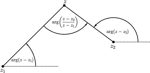
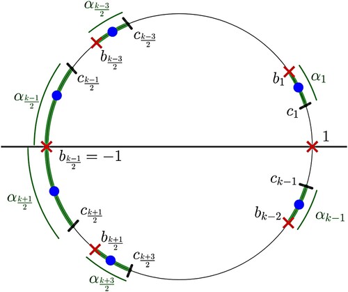
Figure 8. The blue dots are the zeros of and the red cross masks are the zeros of
. By the symmetry of zeros on the unit disc, each element of
has a complex conjugate in
for
. Note that
(
) and
(
).
The following lemma might be a known fact, but since we cannot find it in the literature, we state it here.
Lemma 2.1
Let A be the smaller open arc of bounded by
and
and θ be the angle of the arc A. Let
be the complex conjugates of a and b, respectively. If
,
(depending on the location of the arc A). If
,
(depending on the location of the arc A).
We will use the following theorem found in [Citation4] repeatedly.
Theorem 2.2
[Citation4]
All roots of the polynomial ,
and
for
, are in the interior of the unit ball if and only if
the zeros of
The following lemma will help us when we use Theorem 2.2.
Lemma 2.3
Let and
be real monic polynomials of even degree n with their zeros contained in
. Let
be zeros of
and
be zeros of
, where
(
) and
Let
be the smaller open arc of
bounded by
and
for
. Let θ be a real number such that
. If the arcs
are pairwise disjoint and each element of
has a complex conjugate in
(
), then there is exactly one zero of
(12)
(12) in each
for any positive real number
.
Proof.
The key idea of this proof is found in [Citation10].
First, let and
. Assume that the arcs
are disjoint and each element of
has a complex conjugate in
(
). Define a function
(13)
(13) For fixed
, we claim that
is a continuous real-valued function on each arc
. Let
. Consider
Let
be the angle of the arc
. By Lemma 2.1,
Thus
. This implies
is a negative real number. For
and
, Lemma 2.1 implies
Thus
. This implies
is a positive real number. Hence,
is a negative real number, so
for any
. Then,
is a continuous real-valued function of λ on the arc
. Since
has the values 0 and 1 at the endpoints of the arc
,
must take all values between 0 and 1 on the arc
. By the Intermediate Value Theorem, there exists
such that
. Then,
This implies that
so z is a zero of (Equation12
(12)
(12) ). This means that there exists a zero of (Equation12
(12)
(12) ) in each
for
. Since there are n different zeros of (Equation12
(12)
(12) ), there is exactly one zero of (Equation12
(12)
(12) ) in each
.
In the case that , we consider
instead of
in (Equation13
(13)
(13) ) and proceed with the same method.
3. Classification of sub-triangles for negative feedback
Note that for a positive integer k except at
. Recall also that we define
, where
and
. For a negative feedback system, we have
. For the reader's convenience, we provide a table of symbols in Appendix.
We now consider the stability of oblique sub-triangles.
Theorem 3.1
For negative feedback and , If
, then the sub-triangles
are asymptotically stable, where
.
Proof.
By substituting in Equation (Equation9
(9)
(9) ), eigenvalues of
for sub-triangle
satisfy
and 1 is not an eigenvalue. Let
. In a negative feedback system, we get
. Let
(14)
(14) Our claim is that all roots of
satisfy
. We will use Theorem 2.2 to obtain the claim. First, multiply both sides of (Equation14
(14)
(14) ) by
,
Thus
(15)
(15) Note that
is equal to a polynomial of degree k−1,
except at
. Since we consider
in (Equation15
(15)
(15) ), we have
, so we can refer to both as
. The constant term of
is 1 and the leading coefficient of
is
. Since
, we achieve the first condition of Theorem 2.2.
Let
(16)
(16) Then
(17)
(17) Next, we compute
and
. Since
we get
Hence,
(18)
(18) Similarly,
(19)
(19) To check the second condition of the theorem, we consider two cases of the integer k: it is an odd number and it is an even number.
Case I: k is an odd number.
In this case, can be either an odd or even number. Note that regardless of whether
is an odd number or an even number,
is a zero of
. If
is an odd number, then
is a zero of
since σ is must be an even number, see (Equation16
(16)
(16) ). If
is an even number,
is a zero of
, see (Equation16
(16)
(16) ). Since
and k is an odd number, we can write
where
,
and
are in
,
, and
for
and
. Let
be the smaller arc of
bounded by
and
for
. We use the following lemma which we will prove later.
Lemma 3.2
For every , the arc
contains at most one zero of
.
Since there are k−2 zeros of , by Lemma 3.2 each arc
contains exactly one zero of
. We obtain that
for each i. We may write
(20)
(20) Let
be the smaller open arc of
bounded by
Case II: k is an even number.
In this case, σ and are odd numbers and
Let
Note that
and
have no common zeros and they both have the same degree k−2, which is an even number. We write
where
,
, and
for
. Note that
and
. Let
be the smaller arc of
as follows:
Proof
Proof of Lemma 3.2
Let . Suppose that the arc
contains more than one zero of
, say
has two zeros inside the arc
. Note that the angle of the arc
is greater than the angle of the arc bounded by the two zeros. Then, one of the two zeros is a zero of
and another zero is a zero of
. Let
and
be the two zeros, say
is a zero of
and
is a zero of
. Then, there are
and
such that
Since
and
are contained in arc
,
This implies the following:
(21)
(21) These inequalities are equivalent to
(22)
(22) Adding the inequalities in (Equation22
(22)
(22) ), we get
(23)
(23) Then, l<q + r<l + 1 is a contradiction since q and r are integers.
Figure shows stable sub-triangles (blue shaded sub-triangles) for k = 12 with respect to feedback function . Since
the sub-triangles
,
, and
are asymptotically stable by Theorem 3.1, see Figure .
Figure 9. The boundary sub-triangles for the case of k = 12 and feedback function . The blue sub-triangles are stable.
The following theorem was proved in [Citation23] with a different method.
Theorem 3.3
For negative feedback and , If
, then sub-triangles
and
are asymptotically stable, where
.
Proof.
By substituting and
in (Equation9
(9)
(9) ), the eigenvalues of
for the region
satisfy
(24)
(24) where
. This is equivalent to
(25)
(25) Since
, no zero of Equation (Equation24
(24)
(24) ) lies on the unit circle; i.e.
. If
, then by (Equation25
(25)
(25) )
(26)
(26) a contradiction. Hence,
and then the region
are stable.
Next, the eigenvalues of for the sub-triangle
satisfy
By simplifying, we have
(27)
(27) This is equivalent to
(28)
(28) Note that since
, no solution of quation (Equation27
(27)
(27) ) lies on the unit circle; i.e.
. If
, then by (Equation28
(28)
(28) )
(29)
(29) a contradiction. Hence, the sub-triangle
is stable.
The next corollary is proved by similar ideas as in the proofs of Theorem 3.1. In this corollary, there are some eigenvalues of lying on the unit disc,
.
Corollary 3.4
For negative feedback with the order of events and
, the following statements hold.
If
If
Proof.
Note that (Equation24(24)
(24) ) and (Equation27
(27)
(27) ) are characteristic polynomials for
and
, respectively.
Since , there is a solution of (Equation24
(24)
(24) ) that lies on the unit circle. If
, we get a contradiction as shown in (Equation26
(26)
(26) ). Hence, all solutions of (Equation24
(24)
(24) ) satisfy
. Thus the regions
are neutrally stable.
Equation (Equation27(27)
(27) ) and the condition that
imply that there is a solution of (Equation27
(27)
(27) ) on the unit circle. If
, we get a contradiction as shown in (Equation29
(29)
(29) ). Hence, all solution of (Equation27
(27)
(27) ) satisfy
. We then obtain that
are neutrally stable.
Suppose that . We consider (Equation15
(15)
(15) ) in the proof of Theorem 3.1,
Since
, we have
and
Let
Then,
. We claim that all zeros of
lie in the unit disc. When the claim holds, it follows that no zero of
is outside the units disc, i.e.
. Therefore,
are neutrally stable. Since
, the function
is a polynomial function of degree k−n and
satisfies the first condition of Theorem 2.2. Let
Then,
(30)
(30) Next, we compute
and
defined in Theorem 2.2. Since
we get
Hence,
(31)
(31) Similarly,
(32)
(32) To check the second condition of Theorem 2.2, we consider three cases: k is an odd number, k is an even number and n is an odd number, and, k and n are both even.
Case I: k is an odd number.
This case implies that n is an odd number. Then k−n is an even number. Since σ and cannot be both odd numbers in this case,
is a zero of
. By our construction,
and
have no common zero. We can write
where
,
and
are in
,
, and
for
and
. Now, we write
Let
be the smaller open arc of
bounded by
Case II: k is an even number and n is an odd number.
In this case, σ and are odd numbers, k−n is an even number, and we have
Let
Note that
and
have no common zeros and they both have the same degree k−n−1, which is an even number. We write
where
,
, and
for
. Note that
and
. Let
be the smaller arc of
bounded by
and
for
. Lemma 2.3 implies
has exactly one zero in each
. Hence, all zeros of
lie on
and the zeros of
alternate with the zeros of
for all
. By Theorem 2.2, all zeros of
are in the interior of the unit disc for all
.
Case III: k and n are even numbers.
In this case, σ, , and k−n are even numbers, and we have
Let
Note that
and
have all zeros on
and they have no common zeros. Both
and
have the same degree k−n, which is an even number. We write
where
,
,
, and
for
. Now, let
be the smaller arc of
bounded by
and
for
. Then,
are disjoint and each element of
has a complex conjugate in
(
). Lemma 2.3 implies that
has exactly one zero in each
. Hence, all zeros of
lie on
and the zeros of
alternate with the zeros of
for all
. Therefore, all zeros of
are in the interior of the unit disc for all
.
We prove the following lemma to investigate stability of the boundary sub-triangles corresponding to order of events .
Lemma 3.5
Let k and σ be positive integer satisfying and let
and
, where k + 1−n−m is an even number. Let
If
and
have no common zeros and
are not their zeros, then the function
has all zeros on the unit disc for all
.
Proof.
We write
where
,
, and
for
. Now, let
be the smaller arc of
bounded by
and
for
. Then,
are disjoint and each element of
has a complex conjugate in
for
. If
, Lemma 2.3 implies that
has exactly one zero in each
for
. Hence, all zeros of
lie on
.
Theorem 3.6
For negative feedback with order of events and
, all boundary sub-triangles
,
and
,
are neutrally stable. In particular, all eigenvalues of
for these triangles lie on the unit circle,
.
Proof.
If we substitute or
in (Equation11
(11)
(11) ), the left-hand side of (Equation11
(11)
(11) ) becomes zero. Thus the eigenvalues of
for the regions
and
satisfy
Thus all eigenvalues of
for
and
lie on the unit circle. Hence,
and
are neutrally stable.
Next, let . By substituting
in (Equation11
(11)
(11) ), we obtain that the eigenvalues of
for sub-triangle
satisfy
(33)
(33) Then,
Let
and
. Then,
If
, then there are
such that
,
, and
. Then,
, so
. Thus q = 1. Hence,
. We claim that
has all zeros on the unit disc. There are three possible cases for the variables
and m as follows:
k is odd. This case n, m, σ and
k is even and n is odd. Since
k and n are even. Since
In this case, we obtain that k + 1−n−m is an even number. Moreover, and
have no common zeros and
are not their zeros. By Lemma 3.5, all zeros of
lie on
.
Case II: are even numbers and
are odd numbers.
By Lemma 3.5, all zeros of lie on
.
Case III: k and n are even numbers and are odd numbers.
By Lemma 3.5, all zeros of lie on
.
From this proof, we also get the following corollary:
Corollary 3.7
Let k and σ be positive integers satisfying and let
. The equation
has all solutions on the unit disc.
Thus we have neutrality of boundary triangles, not only for negative feedback but also for positive feedback, provided
.
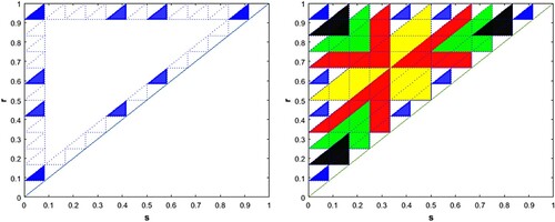
The results in this section identify the location of all asymptotically stable and neutrally stable regions for the boundary sub-triangles. See Figure for an illustration.
Figure 10. Isosequential regions for k = 13 (left) and k = 15 (right) in the limit as . The yellow sub-triangles are neutrally stable by Theorem 3.6. The white sub-triangles are neutrally stable by Corollary 3.4. The blue sub-triangles are asymptotically stable by Theorems 3.1 and 3.3.
We illustrate stability regions of the boundary sub-triangles under negative feedback in Figures and . For a given feedback function and a given k, a program computes vertices of each boundary sub-triangle and uses the results in the previous section to check stability of each sub-triangle. The vertices of each sub-triangle can be computed by a formula presented in the next section.
Figure 11. Illustrations of stability of the boundary sub-triangles for the case of k = 10 with different feedback functions. The first row: feedback functions are and
respectively from the left. The second row:
and
. The blue shaded sub-triangles are stable and the white sub-triangles are neutral.
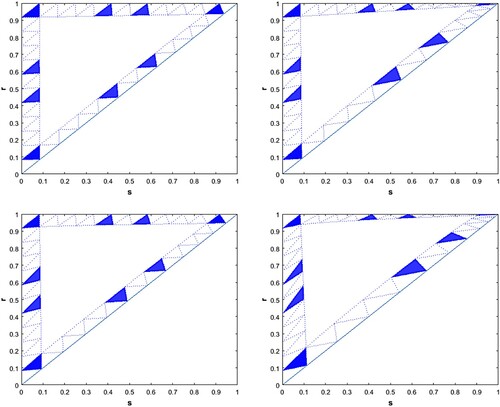
Figure 12. The left column: k = 23 (a prime number). The right column: k = 24 (a composite number). The feedback functions of the figures for each row are the same. The top row: . The middle row:
. The last row:
. The blue shaded sub-triangles are stable and the white sub-triangles are neutral.
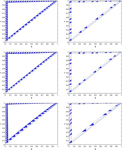
Figure shows the stability of boundary sub-triangles of for the case of k = 10 with different negative feedback functions.
In Figure , we show stability regions for the cases of k = 23 (prime) and k = 24 (composite) under the different negative feedback functions.
We see in these figures that for different feedback functions, the pattern of stability persists, while the sub-triangles become skewed.
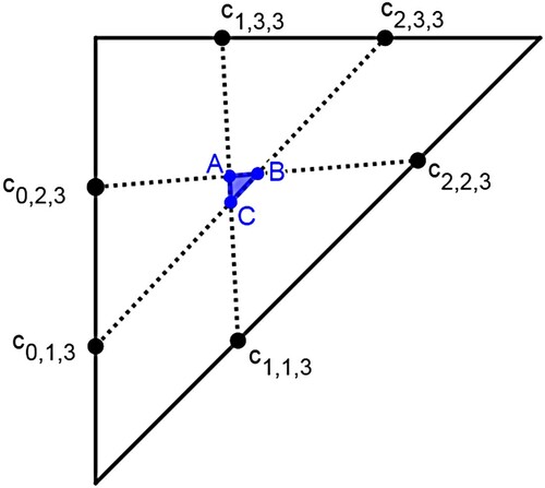
4. The universality of cyclic solutions
In the previous section, we identified which boundary sub-triangles are (asymptotically) stable and which are neutral. In this section, we study how the sub-triangles fit together. For a given linear negative feedback, we prove that the interior of the is covered by the asymptotically stable sub-triangles.
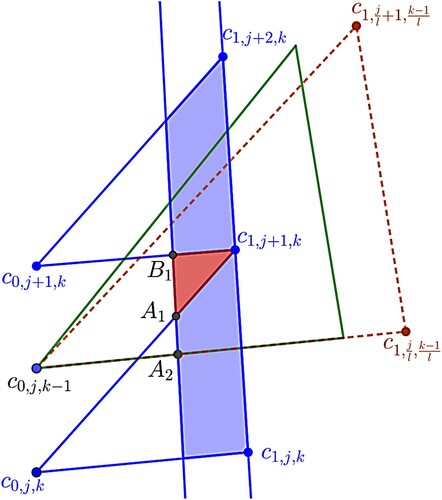
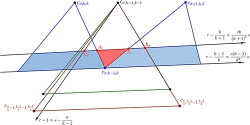
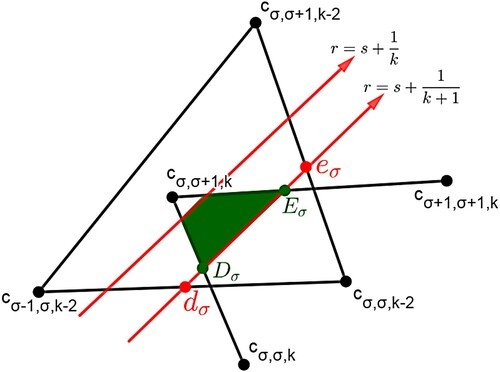
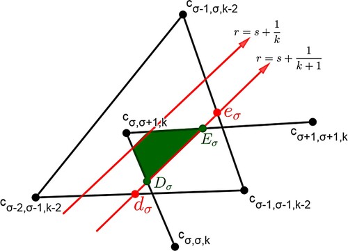
Previously, we saw that an isosequential region has a triangular shape inside and its vertices are simultaneous points [Citation5].
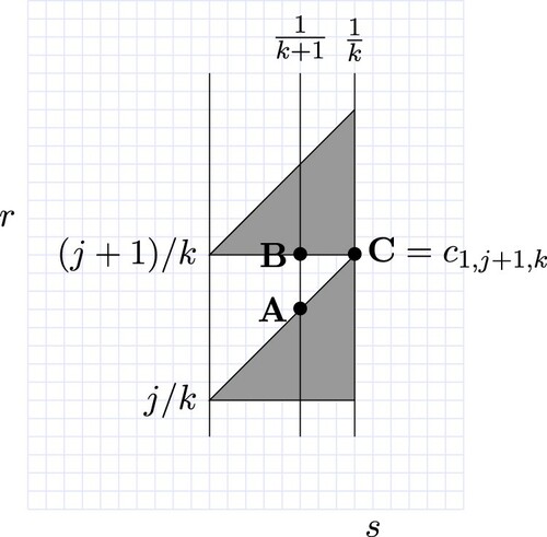
We first find the formula of each simultaneous point. A simultaneous point is a point
in
such that the k-cyclic solution corresponding to the point satisfies the following:
it has events s, r, and 1 occurring simultaneously,
the solution at the initial time has σ clusters in the S region and it has ρ clusters outside the R region.
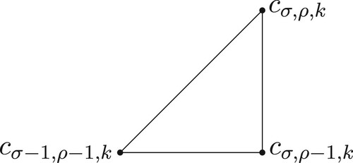
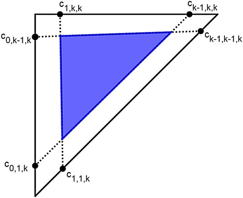
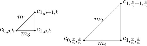
Figure 13. Numbering of the corners of a sub-triangle .
Let be the k-cyclic solution that corresponds to
. We will continue to use
. Then, the k-cyclic solution at the initial time satisfies that
and
. The clusters outside the R region are equally distributed by a distance d (as in Definition 1.1 of k-cyclic solution) and the clusters inside the R region are equally distributed by a distance called
, see Figure . It follows that
. Note that distances outside of R correspond directly to time. Let
be the time required for
to reach
and
be the time for
to reach 1. We will seek conditions for
. Recall that
. Thus
If we require
and since
, we have
Thus
(34)
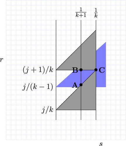
(34) We now consider the case of no feedback, i.e.
for all I. We include this section in order to illustrate some of the main ideas of the proof of Theorem B in a context that is more clear.
Figure 14. The initial location of the k-cyclic solution corresponding to . Here,
and
. The distance between any two adjacent clusters outside the R region is d from Definition 1.1. The distance between any two adjacent clusters inside the R region is
. Note that
because of negative feedback.
With zero feedback, events and isosequential regions are still defined. The formula of each simultaneous point, (Equation34(34)
(34) ), for
becomes simply
(35)
(35)
Definition 4.1
Let k, σ and ρ be positive integers such that and
. A sub-triangle
is a relatively prime sub-triangle if
. If
, sub-triangles
and
are also called relatively prime sub-triangles.
For nonzero negative feedback, relatively prime sub-triangles are the ones that are stable as shown in Theorems 3.1 and 3.3.
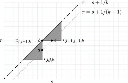
The next lemma is the main idea of the proof. It states that if a boundary triangle is not relatively stable, then it is included entirely inside a larger boundary triangle that is relatively prime. This idea is illustrated in Figure .
Figure 15. Left: , right:
, and
is the slope of each line.
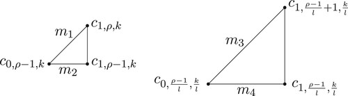
Figure 16. An illustration of Lemma 4.2 for the case k = 12. Left: The boundary sub-triangles for the case of k = 12, where the blue sub-triangles are relatively prime and the white rs1 sub-triangles are not relatively prime. Right: The overlay of relatively prime sub-triangles for k = 2 (yellow), 3 (red), 4 (green) and 6 (black) over k = 12 (blue). The key feature is that these relatively prime sub-triangles perfectly cover the white rs1 boundary sub-triangles on the left.
Lemma 4.2
Let and
. Let
,
,
, and
. Then
(36)
(36)
(37)
(37)
(38)
(38)
Proof.
First, we will prove (Equation36(36)
(36) ). By (Equation35
(35)
(35) ), it follows that
.
In Figure , since the slope and
, it follows that
. Similarly, we can show that
and
For the rest of this section, we assume zero feedback, .
Note that ,
and
are relatively prime sub-triangles. Figure illustrates that all boundary sub-triangles corresponding to order of events rs1 for the case of k = 12 are covered by the relatively prime sub-triangles for
. In the figure,
Let and let
be the triangle which has vertices
,
,
(see Figure ). Then, the following lemma is obvious.
Figure 17. The shaded triangle area is for
.
Lemma 4.3
Consider a zero feedback system. Let be a point in the parameter triangle
. Then there exist a positive integer
and
such that the point
is in the triangle
.
Note here that the following statements hold for :
The next lemma is the second important idea of the proof. We use induction on k to show that for each k, the ‘gap’ is covered by relatively prime sub-triangles. Specifically, the gap is covered by boundary triangles of the form
and
. While not all of these triangles are relatively prime, they are all included perfectly in a larger relatively prime sub-triangle by Lemma 4.2.
Lemma 4.4
Consider a zero feedback system. For a positive integer ,
is covered by relatively prime sub-triangles.
Proof.
We prove this lemma by induction on k. For k = 3, which is a relatively prime sub-triangle. Suppose that
is covered by relatively prime sub-triangles. It suffices to find a relatively prime covering of the gap between
and
, that is the region
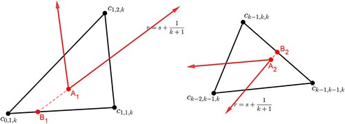
. The gap can be considered as composed of the vertical, horizontal and diagonal gaps. First, we consider the vertical gap between
and
. Let j be a positive integer such that
. Let A be the point on the lines
and
and B be the point on the lines
and
, and C be the point on the lines
and
. We will show below that
is covered by the triangle
. See Figure for a visualization of
.
Figure 18. The vertical gap between and
.
Note that,
(39)
(39) By the definition of points A, B and C, we get
Moreover, the following inequalities hold:
(40)
(40) This inequality implies that the r-coordinate of A is greater than or equal
. Since
(41)
(41) it follows that the slope of line passing
and B is less than or equal to 1. Hence, (Equation39
(39)
(39) ), (Equation40
(40)
(40) ), and (Equation41
(41)
(41) ) imply that
is covered by the sub-triangle
, see Figure . Since
is covered by relatively prime sub-triangle (see (Equation36
(36)
(36) ) in Lemma 4.2), the entire vertical gap between
and
is covered by relatively prime sub-triangles. A similar idea can be used for the horizontal gap.
Figure 19. is covered by the blue triangle
.
Next, we consider the oblique gap, the area inside bounded above by
and bounded below by
, see Figure . Let j be a positive integer such that
. Let a be the point on the lines
and
and b be the point on the lines
and
, and c be the point on the lines
and
. We claim that
is covered by triangle
. See Figure as a visualization of
. Note that
(42)
(42) We get the formulas for the point a, b, c as follows:
Inequality (Equation42
(42)
(42) ) implies that the s-coordinate of c is less than or equal to
. By inequality (Equation40
(40)
(40) ), we have that the r-coordinate of a is greater than or equal to
. Hence,
in Figure is covered by triangle
.
Figure 20. The oblique gap between and
.
Combining Lemmas 4.3 and 4.4, we get the following main theorem.
Theorem 4.5
Consider a zero feedback system. Let be a point in the parameter triangle
. Then there exist a positive integer
such that the point
is in the interior of a relatively prime sub-triangle with respect to the positive integer k.
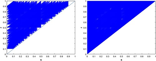
Figure shows that the union of all relatively prime boundary sub-triangles for (left panel) covers a large portion of the interior of
and for
nearly all of
is covered.
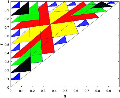
Figure 21. An overlay of all relatively prime sub-triangles for (left) and for
(right) with feedback function
.
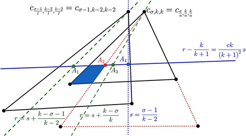
5. Covering under negative linear feedback
In this section, treat negative linear feedback function, for
.
In the previous section, we have proved under the zero feedback that the parameter triangle is covered by relatively prime sub-triangles. The main idea was that boundary sub-triangles that are not relatively prime are included perfectly in larger relatively prime sub-triangles. This fact was used to show that the gap between
and
is covered by a union of relatively prime sub-triangles.
The calculation here is more complicated since the right angle triangles in Section 4 become a scalene triangles under negative linear feedback and Equations (Equation36(36)
(36) ) and (Equation37
(37)
(37) ) in Lemma 4.2 no longer hold. Only the oblique boundary sub-triangles still have this property (Theorem 5.5). For vertical and horizontal sub-triangles, there are thin slices that are not covered by the same larger triangles as in the zero feedback case. The first technical difficulty is showing that these slices are in fact covered by other relatively prime sub-triangles (Lemma 5.9). The second difficulty is showing that these skewed sub-triangles fit together nicely to cover the gap, which is bounded by skewed lines (Lemma 5.10).
Using Equation (Equation34(34)
(34) ), the formula for a simultaneous point
is as follows:
(43)
(43) From this formula, we obtain the following four propositions.
Proposition 5.1
Consider a negative linear feedback system. Let σ and k be positive integers such that . A simultaneous point
for
is a point on the line
This proposition provides the fact that all simultaneous points lie on the same line for fixed σ and
, see Figure (the black line).
Figure 22. Black line: simultaneous points (
) lie on the same line. Blue line: simultaneous points
(
) lie on the same line.
Proposition 5.2
Consider a negative linear feedback system. Let ρ and k be positive integers such that . A simultaneous point
for
is a point on the line
This proposition provides the fact that all simultaneous points lie on the same line for fixed ρ and
, see Figure (the blue line).
Proposition 5.3
Consider a negative linear feedback system. Let ρ and k be positive integers such that . The slope of the line passing through
and
is greater than 1.
Proposition 5.4
Consider a negative linear feedback system. Let σ and k be positive integers such that . The slope of the line passing through
and
is less than 1.
The next result clarifies that any oblique sub-triangle corresponding to the order of events rs1 is covered by stable sub-triangles.
Theorem 5.5
Let f be a negative linear feedback function, where
. For any integer
and
,
where n is a divisor of σ and k.
Proof.
Let n be a positive divisor of σ and k. By (Equation43(43)
(43) ), we get
. Let
be the slope of the line connecting
and
,
be the slope of the line connecting
and
,
be the slope of the line connecting
and
, and
be the slope of the line connecting
and
, see Figure . Using (Equation43
(43)
(43) ), the slopes
,
,
and
are as follows:
and
Therefore,
Figure 23. Left: , right:
.
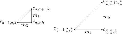
Figure is a visualization of Theorem 5.5 for the case of k = 12 and . The figure indicates that each oblique sub-triangle corresponding to the order of events rs1 for the case of k = 12 and
is exactly covered by a stable sub-triangle for some
.
Figure 24. An overlay of stable sub-triangles for k = 2 (yellow), 3 (red), 4 (green), 6 (black), 12 (blue) where the negative feedback . The oblique sub-triangles for the case of k = 12 are covered perfectly by stable sub-triangles of k = 2, 3, 4, 6. However, the vertical and horizontal sub-triangles for the case of k = 12 are only partially covered. Fully covering these missed slices is a main difficulty of the proof for non-zero feedback.
Definition 5.6
Let k be a positive integer such that . Define
to be the triangle bounded by three line segments defined as follows:
the line passing through
the line passing through
the line passing through
Figure is a visualization of . For a negative linear feedback function
with
, the bounding lines in the sr-plane of the triangle
satisfy:
Figure 25. The blue shaded area is .
The next lemma deals with the gap along the vertical boundary.
Lemma 5.7
Let f be a negative linear feedback function, where
. For
and
, the region
is covered by stable sub-triangles.
Proof.
If , then sub-triangle
is a stable sub-triangle by Theorem 3.3. Thus the theorem holds. Assume that
. Let
, and
be the lines as follows:
Figure 26. Left: , right:
.
Note that . By (Equation43
(43)
(43) ),
,
and
. Then
. Hence,
is partially covered by stable sub-triangle
. Specifically,
can be considered as having two distinct parts; the part that intersects
(the blue shaded area in Figure ) and the part that intersects
(the red shaded region in Figure ). The blue shaded area is covered by the stable triangle
. We claim that the red shaded area is covered by another stable sub-triangle. There are two cases depending on ρ to show that the red shaded area in Figure is covered by a stable sub-triangle.
Figure 27. Red triangle: , blue:
, black vertical line: the vertical boundary of
. The union of the blue- and red shaded regions is
.
Case I: .
Consider sub-triangle where
. We claim that the red shaded area is a subset of
.
Let and
be the following lines:
Figure 28. Sub-triangle . The upper black dot is point A and the lower black dot is B.
To get the claim, we need to show that and the r-coordinate of A is greater than the r-coordinate of B. By (Equation43
(43)
(43) ), the slopes of
,
and
are as follows:
It follows that
. The point A is the solution of the systems
Then, the r-coordinate of A is
(44)
(44) The point B is the solution of the systems
Then, the r-coordinate of B is
We claim that
. By simplification, it is equivalent to show that
(45)
(45) Since
and
, the inequality
(46)
(46) implies the inequality (Equation45
(45)
(45) ). Note that
, so
. Then,
(47)
(47) implies the previous inequality. The left-hand side of the inequality (Equation47
(47)
(47) ) can be considered as a quadratic polynomial
with variable c and fixed k. Then, the following properties hold:
coefficient of
slope of the polynomial is negative at c = 0 and 1,
the values of the function are positive at c = 0 and 1.
Case II: .
In this case, we construct a sub-triangle where
. We claim that the red shaded area is a subset of
. Let D be the line
and the line passing through
and
. Let
and
be slopes of the lines as follows:
Figure 29. Sub-triangle and three lineslopes, m9, m10 and m11. The upper blue dot is point A (same point as in Figure ). The lower black dot is point D, the crossing point between two lines: theline l5 and the line passing through
and
.
The following result addresses the gap along the horizontal boundary.
Lemma 5.8
Let f be a negative linear feedback function, where
. For
and
,
is covered by stable sub-triangles.
Proof.
Let ,
, and
. We consider
as having two distinct parts; the part that intersects
and the part that intersects
. Since
is stable by Theorem 3.3, we need to show that
(the blue shaded region in Figure ) is covered by a stable sub-triangle. The proof will be separated into two cases,
and
.
Figure 30. Case I: . Blue shaded region is
. The red triangle is
.
Case I: . Let
, and
be the following points:
By the definitions of the points and
, we get
It follows that
for
. Since
we get
Case II:
. In this case, we claim that the blue region in Figure is covered by
. Let
be the crossing point between
and the line passing through
and
. We claim that the s-coordinate of point
is less than the s-coordinate of point
. Figure is a visualization of this claim. By Proposition 5.1 and the definition of
, we get
Let
. Then,
Since A<0, it follows that
This inequality implies that
. Therefore, the blue regions covered by stable sub-triangles.
Combining the previous lemmas, we have that sub-triangles in all gaps are covered.
Lemma 5.9
Let f be a negative linear feedback function, where
. For
and
,
,
and
are covered by stable sub-triangles.
The following will confirm that (defined in Definition 5.6) is covered by stable sub-triangles.
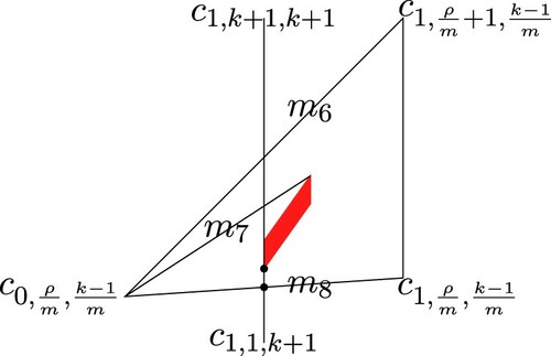
Lemma 5.10
Let f be a negative linear feedback function, where
. For
,
is covered by stable sub-triangles.
Proof.
This lemma will be proved by induction. For k = 3, is shown in Figure , where point A is
, point B is the solution of
and
, and point C is the solution of
and
. Then,
Thus the points A, B, C are in a stable sub-triangle
, i.e. the stable sub-triangle for k = 2.
Figure 31. Case II: . The integer q denotes the greatest common denominator of
and k−1.
Figure 32. The shaded area is . It is covered by the stable sub-triangle
, the largest (yellow) sub-triangle shown in Figure .
It suffices for the inductive step to show that the gap between and
, see Figure , is covered by stable sub-triangles. We separate the gap between
and
into three parts as follows:
The vertical gap is the area bounded by four lines: the line passing through
The horizontal gap is the area bounded by four lines: the line passing through
The oblique gap is the area bounded by four lines: the line passing through
First, we consider the vertical gap and let .Let
. Let
and
be lines as follows:
Figure 33. The gap between and
.
Figure 34. The vertical gap between and
. The blue shaded areas are covered by stable sub-triangles by Lemma 5.9. The green triangle is
. The brown triangle is
where
.
Claim 1
The slope of the line passing through and
is less than or equal 1.
Claim 2
The r-coordinate of is greater than the r-coordinate of
, i.e.
.
We first prove Claim 1. By (Equation43(43)
(43) ), it follows that
is the solution of
(50)
(50) Then, the r-coordinate of
is
(51)
(51) Let
be the s-coordinate of
. Since
, to prove Claim 1 we need to show that
This inequality is equivalent to
by using (Equation50
(50)
(50) ). It is the same as showing
(52)
(52) Since (Equation51
(51)
(51) ) provides the exact value of
, showing (Equation52
(52)
(52) ) is equivalent to prove
(53)
(53) It is equivalent to showing
(54)
(54) Since
and
, the inequality
(55)
(55) implies (Equation54
(54)
(54) ). By multiplying
to (Equation55
(55)
(55) ) and simplifying, we get
(56)
(56) This inequality holds for
. Hence, Claim 1 holds.
Next, we will prove Claim 2, i.e. the r-coordinate of is greater than the r-coordinate of
. Let
and
be the r-coordinates of
and
, respectively. By (Equation43
(43)
(43) ),
is the solution of
Then,
Point
is the solution of
Then,
Showing
is equivalent to prove the following inequality:
(57)
(57) This inequality is equivalent to
(58)
(58) The left-hand side of (Equation58
(58)
(58) ) is a quadratic polynomial function in variable c where
. The polynomial satisfies the following:
the coefficient of
the slopes at c = 0 and c = 1 are both negative,
its values at c = 0 and c = 1 are both positive.
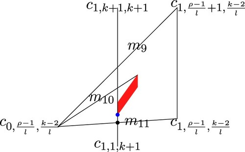
Next, we consider the horizontal gap and let . Let
. Let
, and
be lines as follows:
By Lemma 5.9, the regions and
(the blue shaded areas in Figure ) are covered by stable sub-triangles. We claim that the region bounded by
, and
(the red shaded triangle in Figure ) is covered by
. Let
be the crossing point between
and
,
be the crossing point between
and
,
be the crossing point between
and
, and
be the crossing point between
and
.Since the slope of the line passing through
and
is less than 1 by Proposition 5.4, it suffices to prove the claim by showing that
where
denote the s-coordinates of
,
,
and
, respectively. Figure is a visualization of this claim.
Figure 35. The horizontal gap between and
. The blue shaded areas are covered by stable sub-triangles by Lemma 5.9. The green triangle is
. The brown triangle is
where
.
Point is the solution of
Then,
Point
is the solution of
Then,
Since
is the solution of
we get
Point
is the solution of
Thus
Lemma 5.12 implies
and
. Hence, the red shaded triangle in Figure is covered by
which is a stable sub-triangle. Therefore, the entire horizontal gap between
and
is covered by stable sub-triangles.
Next, we consider the oblique gap between and
. There are four steps to prove how the oblique gap is covered by stable sub-triangles.
Step 1: We will show that the intersection of the vertical and oblique gaps and the intersection of the horizontal and oblique gaps are covered by and
. Let
be the lowest corner of the former intersection and
be the highest corner of the latter intersection. The two red shaded areas in Figure are a visualization of the intersections. We note that the slope of the line segment from
to
is greater than 1. To complete this step, we need to show that
and
. Point
is the solution of
and
Then,
Point
is the solution of
and
Then,
Let be the crossing point of
and the line passing through
and
and let
be the crossing point of
and the line passing through
and
. To show
and
, we need to show that
Figure is a visualization what we need to show. By the definition of
,
and Propositions 5.2 and 5.1, we get the s-coordinates of
and
as follows:
and
Since
we get
. Since
we obtain
This implies
.
Figure 36. The corners of oblique gap between and
where the four green shaded areas called
,
,
,
, respectively from the bottom corner.
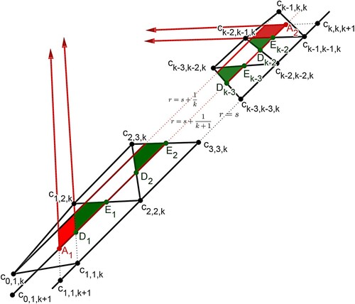
Figure 37. A visualization of the claim to show that and
.
For Steps 2, 3 and 4 below, we define the following:
Step 2: Let . The green regions shown in Figure are a visualization of
,
,
,
. In this step, we claim the following:
(59)
(59) and
(60)
(60)
We first prove (Equation59(59)
(59) ). Let
. Let
be the solution of
and
and let
be the solution of
and
. We claim that the points
and
are in
. Figure is a visualization of this claim. We will prove this by comparing the s-coordinates of the points
and
. Point
is the solution of
and
Then,
The s-coordinate of
is as follows:
By the formulas for
and
, we get
for
. Point
is the solution of
and
Then,
We get the s-coordinate of
as follows:
It is elementary to check that
for
. Then, (Equation59
(59)
(59) ) holds.
Figure 38. A part of the oblique gap between and
for
.
Next, we will prove (Equation60(60)
(60) ). Let
. Let
be the solution of
and
and let
be the solution of
and
.
The s-coordinates of the points are as follows:
Figure is a visualization of
for
. For
, we get
and
. Hence, we get (Equation60
(60)
(60) ).
Figure 39. A part of the oblique gap between and
for
.
Step 3: Let . In this step, we will show that
is covered by
for
. This step will be proved in Lemma 5.11 below.
Step 4: Let and
. In this step, we the proof will depend on the value of c. There are two cases to be considered;
and
.
Case I: . We claim that the points
are in
. Let
be the solution of
and
and let
be the solution of
and
. Figure is a visualization of
. The s-coordinates of
are the following:
(61)
(61)
(62)
(62)
(63)
(63)
(64)
(64) By Lemma 5.13 below, we get
and
. Then, we obtain that
Case II:
. We define the following:
Figure 40. A part of the oblique gap between and
for
and
. The blue shaded region is
.
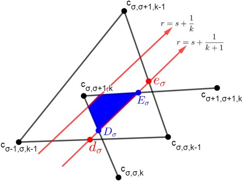
Figure 41. A part of the oblique gap between and
for
and
. The blue shaded region is
.

Point is the solution of
and
Then,
(65)
(65) The s-coordinate of
is as follows:
Point
is the solution of
and
Then,
(66)
(66) The s-coordinate of
is as follows:
By Lemma 5.14 below, we obtain
and
. Then,
By Steps 1-4, the entire oblique gap between
and
is covered by
(67)
(67) By Lemma 5.9, it follows that the set in (Equation67
(67)
(67) ) is covered by stable sub-triangles. Therefore, the entire oblique gap between
and
is covered stable sub-triangles.
We next state and prove the Lemmas 5.11, 5.12, 5.13, and 5.14 that were used above in the proof of Lemma 5.10.
Lemma 5.11
Let f be a negative linear feedback function, where
. Let k and σ be positive numbers,
,
. Then,
(the blue shaded regions in Figure ) defined at the end of Step 1 in the previous lemma is covered by
.
Proof.
By (Equation61(61)
(61) )–(Equation64
(64)
(64) ), the s-coordinates of
,
,
, and
are follows:
The cases
,
can be checked individually [Citation28].
For each case, it follows that and
for any
.
Lemma 5.12
Let k and σ be positive integers such that . Then, the following inequalities hold:
(68)
(68)
(69)
(69) for
.
Proof.
Let . The expression A can be rewritten as a quadratic polynomial in variable c for fixed k and σ:
The polynomial has the following properties:
the coefficient of
its values at c = 0 and c = 1 are both negative,
the slopes at c = 0 and c = 1 are both positive.
Next, we claim that
(70)
(70) Let
For fixed k and σ, B can be rewritten as a quadratic polynomial in variable c:
The polynomial has the following properties:
the coefficient of
its values at c = 0 and c = 1 are both negative,
the slopes at c = 0 and c = 1 are both positive.
Lemma 5.13
Let k and σ be positive integers such that and
. For
, the following inequalities hold:
(71)
(71)
(72)
(72)
Proof.
Let g, h, i be functions on such that
Note that
and
By using the conditions of k and c, it is obvious that
are negative and
are positive. Since
and
are positive,
on
. Since
and
are negative,
on
. Showing
on
is equivalent to showing (Equation71
(71)
(71) ).
Next, let . Then
Since
, we get (Equation72
(72)
(72) ).
Lemma 5.14
Let k and σ be positive integers such that and
. For
, the following inequalities hold:
(73)
(73)
(74)
(74)
Proof.
Let , then
Since
, inequality (Equation73
(73)
(73) ) holds. Let
. Then
Since
, it implies that inequality (Equation74
(74)
(74) ) holds.
Let a point . Then
for some k. By Lemma 5.10, it follows that the point
is covered by a stable sub-triangle. We have now proved Theorem B.
6. Conclusion and discussion
In Theorem thmA, we have fully characterized the stability k-cyclic solutions for in all boundary sub-triangles for any negative feedback. For the order of events sr1 they are always neutrally stable. For the order rs1, the stability is completely determined by the index
or
. Solutions are asymptotically stable if i and k are relatively prime and neutral otherwise.
We have shown in Theorem thmB that for linear negative feedback the stable boundary triangles completely cover the parameter triangle .
Thus the model predicts that there will always exist an asymptotically stable clustered solution regardless of parameter values. Numerics show that this is also true for many forms of nonlinear feedback. See Figures and . In [Citation39], it was shown that for any negative feedback the synchronized solution is unstable. In [Citation2], it was shown that the ‘uniform solution’, i.e. a steady-state periodic solution with cells spread out maximally around the circle is also unstable in most cases. Thus it appears that for negative feedback systems of this form and any parameter values, a k cluster solution will be the only stable periodic solution. This is what we always observe in simulations starting from random initial conditions -- a k cluster periodic solution emerges with roughly the same number of cells in each cluster (see [Citation5] and [Citation32]). The universality of this result is important because for these models, as with many biological systems, the parameter values are hard to estimate from first principles.
Figure 42. An overlay of all stable sub-triangles for (left) and for
(right) with feedback function
.
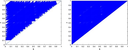
Figure 43. An overlay of all stable sub-triangles for (left) and for
(right) with feedback function
.
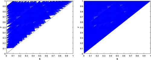
Figure 44. An overlay of all stable sub-triangles for (left) and for
(right) with feedback function
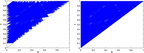
.
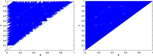
Figure 45. An overlay of all stable sub-triangles for (left) and for
(right) with feedback function
. Note that the graph of this function is S-shaped.
In the following figures, we show visualizations for overlays of stable sub-triangles. The figures were generated using a MATLAB program by the following process:
We first consider linear negative feedback functions and then some examples of nonlinear negative feedback functions.
For each k where
Then, the program displays in one plot all the constructed stable boundary sub-triangles.
For negative linear feedback functions and
, Figures and are overlays of stable regions for
and
.
In Figures and , we show overlays of stable regions for two nonlinear feedback functions and
. For both of these examples and many others that we examined, the parameter triangle is fully covered by stable sub-triangles. Thus we believe that the conclusion of Theorem thmB holds far beyond the linear case.
We note from Figures and and those in this section that most of the area of is already covered with stable sub-triangles with small k. While larger k are theoretically possible, they are expected to be of little consequence for three reasons: (1) the parameter sets where they exist grow small as k increases (they are on the boundary of
), (2) these sets are often overlapped by stability regions with fewer clusters and (3) the amount of feedback exerted by a single cluster would decrease like 1/k as k increases and at some point would be insufficient to overcome the noise in the system. The number of cells, n, in a bioreactor with a litre of fluid is on the order of
, so for practical purposes
.
We observe that there are some negative nonlinear feedback functions such that some points in are not covered by any stable boundary sub-triangle. By Theorems 3.1 and 3.3 and the vertex formula of sub-triangles (Equation34
(34)
(34) ), if there exist a positive integer
and a subset G of
(
is defined in Definition 5.6) such that G is not covered by stable boundary sub-triangles for
, then G is not covered by any stable boundary sub-triangle. For
, Figure suggests that there are regions in
that are not covered by any stable boundary sub-triangles. This feedback function has the features that it is not Lipschitz and it is not bounded below by the functions covered in Theorem thmB. We also observe in Figure that for a particular negative feedback function
that is Lipschitz and bounded below by the function
, the union of stable boundary sub-triangles for all
does not cover the interior of
.
Figure 46. An overlay of all stable sub-triangles for (left) and for
(right) with feedback function
. The white holes in the plot on the right show that for this function not every parameter point is covered by an asymptotically stable boundary sub-triangle.
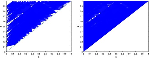
Figure 47. An overlay of all stable sub-triangles for with feedback function
. The white area inside the red circle is the set of points that cannot be covered by any stable boundary sub-triangle since the area is not covered by any stable boundary sub-triangle for
.
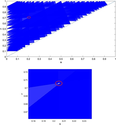
Whether Theorem thmB can be extended more generally is an open question. The numerical results shown in Figures and make it clear that for some non-linear negative feedback functions the stable boundary sub-triangles alone do not fully cover the parameter triangle. As discussed in [Citation2], there are a few exceptional interior sub-triangles that are stable. It is possible that these stable interior sub-triangles cover any holes. In [Citation29,Citation30], the stability of exceptional triangles was proved for k = 9 and . Further, they showed that for k prime, some interior sub-triangles can become stable for larger feedback. The indices of these sub-triangles satisfy certain number theoretic relations. Since the holes in the figures appear only for larger feedback, it is possible that these exceptional sub-triangles cover some or all of the holes.
Numerical simulations, i.e. running the model for some in the holes that appear show that even in the holes in the figures, the solutions always converge to some clustered solution.
In light of these considerations, settling the conjecture fully appears to be complicated.
Disclosure statement
No potential conflict of interest was reported by the author(s).
References
- S. Achuthan and C.C. Canavier, Phase-resetting curves determine synchronization, phase locking, and clustering in networks of neural oscillators, J. Neurosci. 29(16) (2009), pp. 5218–5233.
- B. Bàràny, G. Moses, and T.R. Young, Instability of the steady state solution in cell cycle population structure models with feedback, J. Math. Biol. 78(5) (2019), pp. 1365–1387.
- E.M. Boczko, T. Gedeon, C.C. Stowers, and T.R. Young, ODE, RDE and SDE models of cell cycle dynamics and clustering in yeast, J. Biol. Dyn. 4 (2010), pp. 328–345.
- N. Bose, Tests for Hurwitz and Schur properties of convex combination of complex polynomials, IEEE Trans. Circuits Syst. 36(9) (1989), pp. 1245–1247.
- N. Breitsch, G. Moses, E. Boczko, and T.R. Young, Cell cycle dynamics: Clustering is universal in negative feedback systems, J. Math. Biol. 70(5) (2014), pp. 1151–1175.
- R.L. Buckalew, Mathematical models in cell cycle biology and pulmonary immunity, Ph.D. dissertation, Ohio University, 2014. Available at http://rave.ohiolink.edu/etdc/view?acc_num=ohiou1395242276.
- L. Cai and B.P. Tu, Driving the cell cycle through metabolism, Annu. Rev. Cell Dev. Biol. 28 (2012), pp. 59–87.
- Z. Chen, E.A. Odstrcil, B.P. Tu, and S.L. McKnight, Restriction of DNA replication to the reductive phase of the metabolic cycle protects genome integrity, Science 316 (2007), pp. 1916–1919.
- P. Duboc, L. Marison, and U. von Stockar, Physiology of Saccharomyces cerevisiae during cell cycle oscillations, J. Biotechnol. 51 (1996), pp. 57–72.
- H.J. Fell, On the zeros of convex combinations of polynomials, Pac. J. Math. 89(1) (1980), pp. 43–50.
- B. Fernandez and L. Tsimring, Typical trajectories of coupled degrade-and-fire oscillators: From dispersed populations to massive clustering, J. Math. Biol. 68(7) (2014), pp. 1627–1652.
- R.K. Finn and R.E. Wilson, Population dynamic behavior of the chemostat system, J. Agric. Food Chem. 2 (1954), pp. 66–69.
- B. Futcher, Metabolic cycle, cell cycle and the finishing kick to start, Genome Biol. 7 (2006), pp. 107–111.
- D. Golomb and J. Rinzel, Clustering in globally coupled inhibitory neurons, Physica D 72(3) (1994), pp. 259–282.
- Z.P. Kilpatrick and B. Ermentrout, Sparse gamma rhythms arising through clustering in adapting neuronal networks, PLoS Comput. Biol. 7(11) (2011), p. e10022810.
- I.Z. Kiss, Y. Zhai, and J.L. Hudson, Predicting mutual entrainment of oscillators with experiment-based phase models, Phys. Rev. Lett. 94(24) (2005), p. 248301.
- I.Z. Kiss, C.G. Rusin, H. Kori, and J.L. Hudson, Engineering complex dynamical structures: Sequential patterns and desynchronization, Science 316(5833) (2007), pp. 1886–1889.
- R.R. Klevecz, J. Bolen, G. Forrest, and D.B. Murray, A genome-wide oscillation in transcription gates DNA replication and cell cycle, Proc. Natl. Acad. Sci. USA 101(5) (2004), pp. 1200–1205.
- M.T. Kuenzi and A. Fiechter, Changes in carbohydrate composition and trehalose activity during the budding cycle of Saccharomyces cerevisiae, Arch. Microbiol. 64 (1969), pp. 396–407.
- A. Mauroy and R. Sepulchre, Clustering behaviors in networks of integrate-and-fire oscillators, Chaos18(3) (2008), p. 037122.
- H.K. von Meyenburg, Energetics of the budding cycle of Saccharomyces cerevisiae during glucose limited aerobic growth, Arch. Mikrobiol. 66 (1969), pp. 289–303.
- L. Morgan, G. Moses, and T.R. Young, Coupling of the cell cycle and metabolism in yeast cell-cycle-related oscillations via resource criticality and checkpoint gating, Lett. Biomath. 5 (2018), pp. 113–128. doi:https://doi.org/10.1080/23737867.2018.1456366
- G. Moses, Dynamical systems in biological modeling: Clustering in the cell division cycle of yeast, Ph.D. dissertation, Ohio University, 2015. Available at http://rave.ohiolink.edu/etdc/view?acc_num=ohiou1438170442.
- D. Muller, S. Exler, L. Aguilera-Vazquez, E. Guerrero-Martin, and M. Reuss, Cyclic AMP mediates the cell cycle dynamics of energy metabolism in Saccharomyces cervisiae, Yeast 20 (2003), pp. 351–367.
- T. Munch, B. Sonnleitner, and A. Fiechter, The decisive role of the Saccharomyces cervisiae cell cycle behavior for dynamic growth characterization, J. Biotechnol. 22 (1992), pp. 329–352.
- L.L. Newcomb, J.A. Diderich, M.G. Slattery, and W. Heideman, Glucose regulation of Saccharomyces cerevisiae cell cycle genes, Eukaryot. Cell 2 (2003), pp. 143–149.
- P.R. Patnaik, Oscillatory metabolism of Saccharomyces cerevisiae: An overview of mechanisms and models, Biotech. Adv. 21 (2003), pp. 183–192.
- K. Prathom, Stability regions of cyclic solutions under negative feedback and uniqueness of periodic solutions for uneven cluster systems, Ph.D. dissertation, Ohio University, 2019. Available at https://etd.ohiolink.edu/etdc/view?acc_num=ohiou1562778288743268.
- K.C. Rabi, Study of some biologically relevant dynamical system models: (In)stability regions of cyclic solutions in cell cycle population structure model under negative feedback and random connectivities in multi-type neuronal network models, Ph.D. dissertation, Ohio University, 2020. Available at http://rave.ohiolink.edu/etdc/view?acc_num=ohiou16049254273607.
- K.C. Rabi, A. Algoud, and T.R. Young, Instability of k-cluster solutions in a cell cycle population model when k is prime, J. Appl. Nonlinear Dyn. 11(1) (2022), pp. 87–138.
- J.B. Robertson, C.C. Stowers, E.M. Boczko, and C.H. Johnson, Real-time luminescence monitoring of cell-cycle and respiratory oscillations in yeast, Proc. Natl. Acad. Sci. USA 105 (2008), pp. 17988–17993.
- J. Rombouts, K. Prathom, and T. Young, Clusters tend to be of equal size in a negative feedback population model of cell cycle dynamics, SIAM J. Appl. Dyn. Syst. 19(2) (2020), pp. 1540–1573. doi:https://doi.org/10.1137/19M129070X
- C. Stowers, T.R. Young, and E. Boczko, The structure of populations of budding yeast in response to feedback, Hypoth. Life Sci. 1(3) (2011), pp. 71–84.
- A.F. Taylor, P. Kapetanopoulos, B.J. Whitaker, R. Toth, L. Bull, and M.R. Tinsley, Clusters and switchers in globally coupled photochemical oscillators, Phys. Rev. Lett. 100(21) (2008), p. 214101.
- A. Taylor, M. Tinsley, and K. Showalter, Insights into collective cell behaviour from populations of coupled chemical oscillators, Phys. Chem. Chem. Phys. 17(31) (2015), pp. 20047–20055.
- K. Uchiyama, M. Morimoto, Y. Yokoyama, and S. Shioya, Cell cycle dependency of rice α-amylase production in a recombinant yeast, Biotechnol. Bioeng. 54 (1996), pp. 262–271.
- M. Wickramasinghe and I.Z. Kiss, Spatially organized dynamical states in chemical oscillator networks: Synchronization, dynamical differentiation, and chimera patterns, PLoS ONE 8(11) (2013), p. e80586.
- D. Wilson and J. Moehlis, Clustered desynchronization, from high-frequency deep brain stimulation, PLoS Comput. Biol. 11 (2015), p. e1004673.
- T.R. Young, B. Fernandez, R. Buckalew, G. Moses, and E.M. Boczko, Clustering in cell cycle dynamics with general response/signaling feedback, J. Theor. Biol. 292 (2012), pp. 103–115.
- J. Zhang, Z. Yuan, and T. Zhou, Synchronization and clustering of synthetic genetic networks: A role for CIS-regulatory modules, Phys. Rev. E 79 (2009), p. e041903.
- G. Zhao, Y. Chen, L. Carey, and B. Futcher, Cyclin-dependent kinase co-ordinates carbohydrate metabolism and cell cycle in S. cerevisiae, Mol. Cell 62 (2016), pp. 546–557.
Appendix. List of symbols
| = | coordinate of a cell | |
| = | coordinate of a cluster | |
| = | initial condition of a cluster, i.e. | |
| k | = | number of clusters in the cell cycle |
| S | = | interval |
| R | = | interval |
| σ | = | number of clusters inside S at the initial time |
| ρ | = | number of clusters in |
| = | feedback function | |
| = | a particular value of the feedback function when σ clusters are in the S region, from the total number of k clusters | |
| = | ||
| = | ||
| Π | = | Poincaré return map for the system with clusters |
| F | = | partial return map, a factor of Π |
| = | parameter triangle, set of points | |
| = | sub-triangle (isosequential region) corresponding to the k-cyclic solutions with order of events | |
| = | sub-triangle corresponding to the k-cyclic solutions with order of events | |
| = | triangle bounded by |