
 ?Mathematical formulae have been encoded as MathML and are displayed in this HTML version using MathJax in order to improve their display. Uncheck the box to turn MathJax off. This feature requires Javascript. Click on a formula to zoom.
Abstract
In a recent paper, Che et al. [5] used a continuous-time Ordinary Differential Equation (ODE) model with risk structure to study cholera infections in Cameroon. However, the population and the reported cholera cases in Cameroon are censored at discrete-time annual intervals. In this paper, unlike in [5], we introduce a discrete-time risk-structured cholera model with no spatial structure. We use our discrete-time demographic equation to ‘fit’ the annual population of Cameroon. Furthermore, we use our fitted discrete-time model to capture the annually reported cholera cases from 1987 to 2004 and to study the impact of vaccination, treatment and improved sanitation on the number of cholera infections from 2004 to 2019. Our discrete-time cholera model confirms the results of the ODE model in [5]. However, our discrete-time model predicts a decrease in the number of cholera cases in a shorter period of cholera intervention (2004–2019) as compared to the ODE model's period of intervention (2004–2022).
1. Introduction
According to the World Health Organization (WHO), cholera is an acute intestinal infection caused by ingestion of food or water contaminated with the bacterium Vibrio cholerae [Citation26]. In many parts of the world, cholera remains a significant threat to public health [Citation25]. It continues to devastate impoverished populations with limited access to medication, clean water and proper sanitation amenities [Citation16]. Annually, about 1.3 to 4.0 million cholera cases and 21, 000 to 143, 000 cholera-induced deaths are reported worldwide [Citation1,Citation26]. In recent years, there have been several reports of major cholera outbreaks. For example, in Haiti from 2010 to 2012 there were more than 530,000 reported cases [Citation16]. Major outbreaks were also reported in Sierra Leone (2012), Ghana (2011), Nigeria (2010), Vietnam (2009), Zimbabwe (2008), and India (2007). Cameroon, a cholera endemic African country experienced large cholera outbreaks in 1991, 1996, 1998, 2004, 2010 and 2011 [Citation19]. In 2017, 1,227,391 cases and 5,654 deaths of cholera were reported from34 countries [Citation24].
Transmission of cholera can be indirect, from water infected with the bacterium to susceptible humans, or direct, from infectious humans to susceptible humans [Citation18,Citation20,Citation23]. Several continuous-time mathematical ODE models have been developed, in an effort to gain a deeper understanding of cholera transmission dynamics, see [Citation23] and the citations therein. In a recent paper, Che et al. introduced a continuous-time ODE low–high risk-structured cholera model and used it to capture the annual reported cholera infections in Cameroon from 1987 to 2017 [Citation5].
The cholera census data used in [Citation5] were reported annually [Citation27]. Thus, unlike the ODE cholera model in [Citation5], to capture the annual census data in Cameroon, in this paper, we introduce a discrete-time low-high risk-structured cholera model of Cameroon. That is, as in the reported annual cholera data of Cameroon, we assume that the unit time interval is 1 year and we use the knowledge of the population sizes at time t to predict the population sizes at time . We will use our discrete-time model's demographic equation to ‘fit’ the population of Cameroon, and then use the fitted discrete-time cholera model to capture reported annual cholera cases in Cameroon from 1987 to 2004. Furthermore, as in [Citation5], we will use our model to study the impact of three cholera intervention strategies (vaccination, treatment, and sanitation) on the number of cholera infections in Cameroon from 2004. Also, we will use our model to predict future cholera cases in Cameroon.
Both the continuous-time and discrete-time cholera models of Cameroon are based on observations and assumptions of the cholera disease dynamics in Cameroon. However, unlike the continuous-time model, the discrete-time model is also based on the observation that the cholera cases in Cameroon are reported annually. Thus, the difference equations of our novel discrete-time model are a closer fit to the observed cholera cases in Cameroon than the ordinary differential equations of the continuous-time choleramodel.
Discrete-time disease epidemic models are ubiquitous in the literature [Citation4,Citation10,Citation13,Citation21,Citation22,Citation28]. For example, van den Driessche and Yakubu, in [Citation22], introduced a discrete-time SIR-B cholera model with direct and indirect cholera transmission pathways. Our discrete-time risk-structured cholera model, unlike the model in [Citation22], partitions the entire Cameroon population into two cholera risk groups; ‘low’ and ‘high’ cholera risk groups.
The rest of the paper is organized as follows: In Section 2, we identify the low and high cholera risk groups in Cameroon and then introduce our discrete-time risk-structured model with no disease intervention. We compute the discrete-time demographic threshold parameter, , and then use our model's discrete-time demographic equation to ‘fit’ the census data of the population of Cameroon. We compute the basic reproduction number,
, and then use the fitted discrete-time risk-structured model to capture reported cholera cases in Cameroon from 1987 to 2004. Also, in Section 2, we use sensitivity analysis to study the impact of our model parameters on
,
, and on the total number of our model's predicted cholera cases. In Section 3, we study the impact of vaccination, treatment and sanitation as cholera intervention strategies on the number of cholera infections in Cameroon from 2004 to 2019. We compute the effective reproduction number,
, and use sensitivity analysis to study the impact of our model parameters on
and on the total number of predicted cholera cases by our model with intervention. In Section 4, we compare the results of our discrete-time cholera model of Cameroon to that of the corresponding continuous-time ODE Cholera model in [Citation5]. Our conclusions are in Section 5.
2. Model formulation
In [Citation5], Che et al. partitioned the ten regions of Cameroon, shown in Figure , into ‘low’ and ‘high’ risk cholera regions, see Table . Unlike in [Citation5], we use the two risk groups to construct a discrete-time structured cholera model. Also, in [Citation5], Che et al. used their scaled cholera model to capture scaled values of the 1987–2017 Cameroon's yearly reported cholera cases from WHO [Citation27]. The scaled values are obtained by dividing the yearly reported cholera cases from [Citation27] by the Cameroon population census data [Citation17], see Figure . As in [Citation5], we will use our discrete-time model to capture the actual cholera cases. First, we introduce the discrete-time demographic equation and use it to capture the 1987–2017 Cameroon's population census data from the World Bank [Citation17].
Figure 1. Map of Cameroon showing the ten regions and neighbouring countries [Citation15].
![Figure 1. Map of Cameroon showing the ten regions and neighbouring countries [Citation15].](/cms/asset/7c81b06b-6106-491b-b8b6-ff1cb5e948b1/tjbd_a_1991497_f0001_oc.jpg)
Figure 2. Scaled values of the yearly reported cases of cholera in Cameroon from 1987 to 2017. The scaled values are obtained by dividing the yearly reported cholera cases from [Citation27] by the Cameroon population census data [Citation17].
![Figure 2. Scaled values of the yearly reported cases of cholera in Cameroon from 1987 to 2017. The scaled values are obtained by dividing the yearly reported cholera cases from [Citation27] by the Cameroon population census data [Citation17].](/cms/asset/81caeb19-a91f-4cdf-95ba-b46458a4fe87/tjbd_a_1991497_f0002_oc.jpg)
Table 1. Low- and high-risk regions of Cameroon.
2.1. Demographic equation and Cameroon population
To introduce the discrete-time demographic equation, we let denote the total population of Cameroon, at time
. The population of Cameroon is modelled by the difference equation
(1)
(1) where the parameters β, natural birth rate, and δ, natural death rate, are determined from the Cameroon's population census data [Citation17]. In Model (Equation1
(1)
(1) ), time is in years. The first term denotes the recruitment (birth) function of individuals into the population per year and the second time is the proportion of those that survive per year. We take t = 0 to correspond to 1987, t = 1 is 1988, and so on. Consequently, the initial condition
is the population of Cameroon in 1987, rounded to the nearest ten thousand (see [Citation17]). Model (Equation1
(1)
(1) ) has a dimensionless demographic threshold parameter
The total population goes extinct when
while it persists when
.
In [Citation5], Che et al. estimated that the birth rate per year, , and the death rate per year,
. Consequently, as in [Citation5],
. Hence,
and
imply that the population of Cameroon is experiencing exponential growth.
Let
Then
is the constant per capital growth rate.
A scatter plot of the Cameroon population census data in [Citation17] and a plot of the solution of (Equation1
(1)
(1) ) using the estimates of β and δ are shown in Figure . From Figure , the solution
of Model (Equation1
(1)
(1) ) fits the Cameroon population census data with relative error
, where as in [Citation5]
is the vector of the number of yearly population given by Model (Equation1
(1)
(1) ) and
is the vector of the actual number of the yearly population [Citation17]. The scalar value
is the square root of the sum of the squares of the differences between the model results and the actual population data at the corresponding times, and
is the square root of the sum of the squares of the actual population data for each year.
Figure 3. Scatterplot of Cameroon census data for years 1987–2017 [Citation17] versus ‘fitted’ Model (Equation1(1)
(1) ) solution. The model solution
is shown as asterisks, and the dots are the data.
fits the Cameroon population data with relative error
.
![Figure 3. Scatterplot of Cameroon census data for years 1987–2017 [Citation17] versus ‘fitted’ Model (Equation1(1) N(t+1)=βN(t)+(1−δ)N(t)=(β+(1−δ))N(t),(1) ) solution. The model solution N(t) is shown as asterisks, and the dots are the data. N(t) fits the Cameroon population data with relative error =8.2652×10⁻³.](/cms/asset/4fb47e7d-0723-4439-8e98-0a1c9ada03dd/tjbd_a_1991497_f0003_oc.jpg)
2.2. Low–high-risk structured cholera model
Based on the schematic diagram shown in Figure , we introduce a simple risk-stratified discrete-time model of cholera infections in Cameroon with no explicit spatial structure. The list of the model variables and their descriptions are in Table , while the parameters are in Table .
Figure 4. Flow diagram for the risk-structured model. Solid lines represent flow between compartments, the straight dashed line represents the infectious class shedding pathogen into the environment and the curved dashed line represents the source of infections resulting from susceptibles interacting with the pathogen.
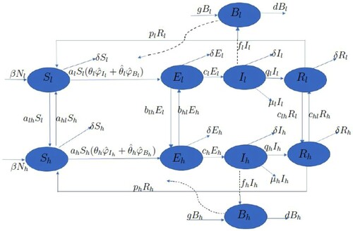
Table 2. Model variables, descriptions and units.
Table 3. Model parameters, descriptions and values.
At time we denote by
,
, and
the population sizes of the susceptible, exposed, infectious, and recovered low-risk individuals, respectively. The total population size of the low-risk subpopulation at time t is
Also, we denote by
,
, and
the population sizes of the susceptible, exposed, infectious, and recovered high-risk individuals at time
respectively. Similarly, the total population size of the high-risk subpopulation at time
is
The total population of individuals in the two risk groups at time
is
At time
we denote by
and
the concentration of pathogens in the contaminated water in the low-risk and high-risk environments, respectively.
In each risk group , we assume that a fraction
of susceptible individuals, become exposed via contact with infectious individuals (direct transmission) with probability
and a fraction
of susceptible individuals, become exposed via contact with contaminated water (indirect transmission) with probability
The ‘escape from direct infection’ and ‘escape from indirect infection’ functions are, respectively, the nonlinear decreasing smooth concave-up functions
and
where
. That is, for all
,
and
If, for example, the interactions between susceptible individuals and infectious individuals or susceptible individuals and the contaminated water are modelled as Poisson processes, then
(2)
(2) and
(3)
(3) where the parameters
and
are the transmission rates between susceptible individuals and infectious individuals, and susceptible individuals and contaminated water, respectively (see Table ).
For each unit time interval , and in each risk group
, the fraction of exposed individuals that can progress to the infectious class is
and the fraction that remains in the exposed class is
. Infectious individuals can contaminate the water by shedding the pathogen at a positive rate
per unit time interval
. We assume that in Cameroon, the number of cholera infections from cholera infected corpses is very small and can be ignored. Cholera is a treatable disease. In Cameroon cholera is usually treated with oral rehydration salt solutions and antibiotics. In our model, for each unit time interval
, the fraction of infectious individuals that can progress to the recovered class is
and the fraction that remains in the infectious class is
. The fraction of infectious individuals that can die from cholera infection is
. We assume that
, so that per unit time interval
, the fraction of infectious individuals that die from other causes does not exceed the fraction that do not die from cholera infection. Recovered individuals do not have permanent immunity, and so the fraction that can become susceptible to the infection is
. In the pathogen class, a fraction
of cholera pathogen is added (growth) and a fraction
is removed from the water (decay).
Our model allows for the movement of individuals between the two risk groups. For each unit time interval , the fraction of susceptible individuals that can move from the low-risk group to the high-risk group is
, and the fraction of susceptible individuals that can move from the high-risk group to the low-risk group is
. The fraction of exposed individuals that can move from the low-risk group to the high-risk group is
, and the fraction of exposed individuals that can move from the high-risk group to the low-risk group is
. We assume that
, so that the fraction of exposed individuals that can move from the low-risk group to the high-risk group does not exceed the fraction that does not become infectious in the low-risk group. Also, we assume that
, so that the fraction of exposed individuals that can move from the high-risk group to the low-risk group does not exceed the fraction that does not become infectious in the high-risk group. The fraction of recovered individuals that can move from the low-risk group to the high-risk group is
, and the fraction of exposed individuals that can move from the high-risk group to the low-risk group is
. We assume that
, so that the fraction of recovered individuals that can move from the low-risk group to the high-risk group does not exceed the fraction that does not lose their immunity in the low-risk group. We assume that
, so that the fraction of recovered individuals that can move from the high-risk group to the low-risk group does not exceed the fraction that does not lose their immunity in the high-risk group. However, we assume that infectious individuals are too sick to move and are confined to their respective risk groups. The simple mathematical model for the spread of the disease in the two risk groups with movements of non-infectious individuals between the groups is thus given by the following system of difference equations:
(4)
(4) with initial conditions:
and
In Figure , we have set
and
We note that all the terms in our structured Model (Equation4
(4)
(4) ) are nonnegative. In fact, starting with initial conditions
and
we have
and
for all
For each risk group , in the absence of shedding of the Vibrio cholerae, the pathogen equations in Model (Equation4
(4)
(4) ) reduce to the following difference equation
Consequently, when d<g then the pathogen maintains itself in the environment via geometric growth. In the absence of shedding, to exclude pathogen population explosion in the Cameroon environment, we assume that d>g. That is,
is the net decay rate of the pathogen. Summing the equations for
and
, we obtain
(5)
(5) In the absence of cholera infections,
, and (Equation5
(5)
(5) ) reduces to (Equation1
(1)
(1) ), the demographic equation of Cameroon. Let
To consider proportions,we let
and
for
Also, we let
for
Model (Equation4
(4)
(4) ) becomes
(6)
(6) where
and
for
.
We can rewrite Equation (Equation5(5)
(5) ) as
In Cameroon,
,
and
. So,
Moreover, in Cameroon, the population is growing exponentially. So,
for
. Thus,
. With
and
we see that in Model (Equation6
(6)
(6) ),
and
for
.
Since and
, for
the equation for
and
in Model (Equation6
(6)
(6) ) implies
and
To obtain the feasible region of solutions to Model (Equation6
(6)
(6) ), we consider the first-order linear difference equations
and
Recall that
. Let
and
For each risk group
, we let
Assuming
for all
, the feasible region of solutions of Model (Equation6
(6)
(6) ) is the compact set
2.3. Structured model: DFE and 
Model (Equation6(6)
(6) ) has a trivial disease-free equilibrium point (DFE),
and a non-trivial DFE,
For Cameroon,
and the trivial equilibrium,
, is unstable. Now, for
we use the next generation matrix (NGM) method to compute
, the basic reproduction number of Model (Equation6
(6)
(6) ) [Citation2,Citation22]. Assuming that
and
are not new infections, we obtain that F, the matrix of new infections, is
where
and T, the matrix of transition terms, is
Thus,
, the spectral radius of
, is
(7)
(7) where
In Model (Equation6
(6)
(6) )
implies the DFE,
, is locally asymptotically stable and cholera is eliminated in Cameroon. However,
implies
is unstable and cholera invades the Cameroon population.
In Cameroon, reported cholera interventions began in 2004 [Citation9]. To compute for Cameroon, in the next subsection, we use the scaled values of pre-intervention Cameroon's yearly reported cholera cases from 1987–2004 (see Figure ) to estimate the remaining Model (Equation6
(6)
(6) ) parameter values. We will use the fitted Model (Equation6
(6)
(6) ) to illustrate that in Cameroon,
and cholera is an endemic infectious disease.
2.4. Structured model: parameter estimation
As in Section 2.1, we take year
and
year
. For the transmission rate between susceptible and infectious individuals in the low-risk group,
[Citation22]. For the fraction of infectious individuals in the low-risk group who can die due to cholera infection, we multiply the cholera-related death rate per day in [Citation5] by 365 days to obtain
per year, that is
. For the fraction of infectious individuals in the high-risk group who can die due to cholera infection, we multiply the cholera-related death rate per day in [Citation5] by 365 days to obtain
per year, that
. For the fraction of recovered individuals that can transition from the low-risk group to the high-risk group, we multiply the transition rate per day in [Citation5] by 365 days to obtain
per year, that is
. For the fraction of recovered individuals that can transition from the high-risk group to the low-risk group, we multiply the transition rate per day in [Citation5] by 365 days to obtain
per year, that is
.
As in [Citation5], we estimate the remaining model parameters using the multistart algorithm with the fmincon function in the MATLAB optimization toolbox. The fmincon function takes an iterative approach to solving an optimization problem that includes our parameter values as unknowns with the scalar value to be minimized being the relative error,
(8)
(8) where
is the vector of the number of yearly new infections given by the structured Model (Equation6
(6)
(6) ) with parameter vector m, and
is the corresponding vector of the scaled values of the yearly reported cholera cases [Citation27]. The scaled values are obtained by dividing the yearly cholera cases by the yearly population data [Citation17].
There are more job, educational and trade opportunities in the high risk regions than the low-risk regions. Consequently, more people tend to move from the low-risk regions to the high-risk regions in search of those opportunities. To capture this movement pattern in the structured Model (Equation6(6)
(6) ), as in [Citation5], we choose
and
, (see Table ).
For the initial conditions, we take . As in [Citation5], we assume that the high-risk population is about three times that of the low-risk population. Consequently, for the low-risk population, we let
,
,
,
and
. Recall that
For the high-risk population, we let
,
,
,
and
. Similarly,
As noted in [Citation5],
percent of the total population of Cameroon in 1987 is high risk. To ensure that a higher fraction of individuals in the
class are infected than the individuals in the
class, as in [Citation5], we choose
,
,
and
so that
and
(see Table ).
We do not have data for the 1987 pathogen concentrations in the low and high-risk regions, and
, respectively. As in the continuous-time ODE model, we take
Also, we let
and
be defined as in (Equation2
(2)
(2) ) and (Equation3
(3)
(3) ). Using pre-intervention observations for Cameroon population, with
,
,
year
and
year
, we estimate the remaining parameter values for
(see Table ). Using these parameter values and Equation (Equation7
(7)
(7) ), we estimate that
. In [Citation5], Che et al. used their ODE model to obtain
for cholera disease in Cameroon. Thus, as in [Citation5], our discrete-time risk-structured cholera model correctly predicts cholera endemicity in Cameroon.
In [Citation5], we obtained that with a relative error of 0.8637, the continuous-time ODE structured model captures the known cholera endemicity in Cameroon, while predicting a decreasing trend from 1987 to 1994 and an increasing trend from 1995 to 2004 in the pre-intervention reported number of cholera cases in Cameroon from 1987 to 2004. Figure shows the resulting Model (Equation6(6)
(6) ) output values of the yearly number of new cholera infections predicted by the scaled structured model in comparison with the scaled values of the actual yearly cholera reported cases in Cameroon from 1987–2004, see Figure . From Figure , we see that unlike the continuous-time ODE model in [Citation5], with a relative error of 0.8441, our discrete-time risk-structured model captures the known cholera endemicity in Cameroon, and predicts an increasing trend from 1987 to 1989, 1990 to 1992, 1993 to 1995, 1997 to 1998 and 2003 to 2004, and a decreasing trend from 1989 to 1990, 1992 to 1993, 1995 to 1997 and 1998 to 2003.
Figure 5. Scatterplot of the yearly cholera disease cases in Cameroon for 1987-2004 from [Citation27] plotted against simulation output using estimated parameters. With a relative error of 0.8441, the structured model captures the known cholera endemicity in Cameroon, and predicts an increasing trend from 1987 to 1989, 1990 to 1992, 1993 to 1995, 1997 to 1998 and 2003 to 2004, and a decreasing trend from 1989 to 1990, 1992 to 1993, 1995 to 1997 and 1998 to 2003.
![Figure 5. Scatterplot of the yearly cholera disease cases in Cameroon for 1987-2004 from [Citation27] plotted against simulation output using estimated parameters. With a relative error of 0.8441, the structured model captures the known cholera endemicity in Cameroon, and predicts an increasing trend from 1987 to 1989, 1990 to 1992, 1993 to 1995, 1997 to 1998 and 2003 to 2004, and a decreasing trend from 1989 to 1990, 1992 to 1993, 1995 to 1997 and 1998 to 2003.](/cms/asset/c10b8619-f4b6-4f6f-8454-e3657e484f66/tjbd_a_1991497_f0005_oc.jpg)
2.5. Sensitivity analysis
In this section, we use sensitivity analysis to study the impact of each model parameter on the threshold parameters, and
and the number of model predicted cholera cases. For a variable v and a parameter p, the analytic sensitivity index to the parameter p is defined as
This index gives the proportional rate of change of v as p changes [Citation6]. A positive index will mean that an increase in the variable p will lead to a proportional increase in v, and a negative index will mean an increase in p will lead to a proportional decrease in v. We have
and
So, as in [Citation5], the sensitivity indices of
, the demographic threshold of Cameroon, do not depend on either β or δ, the parameters of (Equation1
(1)
(1) ).
2.5.1. Sensitivity indices of
Next, we compute the sensitivity indices for with respect to each of the 25 structured Model (Equation6
(6)
(6) ) parameters of Table . Most of the sensitivity indices are complicated algebraic expressions with no obvious structure. As in [Citation6], we evaluate the sensitivity indices at the baseline parameter values given in Table . Table summarizes our results with the parameters ordered from the most sensitive to the least sensitive. Unlike the ODE model in [Citation5], where the most sensitive parameter is
, the recovery rate of infectious individuals in the high-risk group, in our discrete-time model,
, and the most sensitive parameter is
, the contact rate between the susceptible individuals and the cholera pathogen in the high-risk group (see Table ). Thus, decreasing (or increasing) the most sensitive parameter
, by
decreases (or increases)
by
. Also, from Table ,
. So, another important parameter in our discrete-time model is
, the fraction of exposed individuals in the high-risk group that can progress to the infectious class. Thus, increasing (or decreasing)
by
increases (or decreases)
by
. The least sensitive parameters in our discrete-time model are
and
, the fraction of recovered individuals in the high-risk group who become susceptible, and
and
, the fraction of recovered individuals who transition from the low-risk group to the high-risk group and from the high-risk group to the low-risk groups, respectively. Because
decreasing (or increasing)
,
,
or
by
does not affect
.
Table 4. Sensitivity indices of with respect to the 25 structured Model (Equation6
(6)
(6) ) parameters, evaluated at the baseline parameter values given in Table .
2.5.2. Global sensitivity analysis
Next, as in the ODE model in [Citation5], we perform a global sensitivity analysis for our model using Latin Hypercube Sampling (LHS) to sample the parameter space and Partial Rank Correlation Coefficients (PRCC) to evaluate the sensitivity of the outcome variable, the total number of model predicted cholera cases, to uncertainty in the input variables [Citation3,Citation7,Citation12]. For parameter intervals, as in [Citation5], we pick values above and below the values in Table . Uniform probability distributions were used for each parameter interval. From the recommendation in [Citation14], we take
draws of the LHS design, where M, the number of input parameters is 25 and N, the number of LHS draws is 50.
Table gives the PRCCs and the p-values for each model parameter while Figure shows the sensitivity of the number of cholera cases to changes in parameters in Table as computed by the Latin Hypercube Sampling-Partial Rank Correlation Coefficient (LHS-PRCC) index. Based on the p-values, we observe that PRCC values for , 0.5440, for
, 0.7091 and for
, 0.7054 are statistically significant. As compared to the ODE model in [Citation5], where
, the scaled contact rate between susceptible individuals and the cholera pathogen in the high-risk group shows a significant positive correlation with the total number of cholera cases and
, the recovery rate of infectious individuals in the high-risk group shows a significant negative correlation with the total number of cholera cases, in our discrete-time model,
, the contact rate between susceptible individuals and the cholera pathogen in the high risk,
, the fraction of exposed individuals that can progress to the infectious class and
, the shedding rate of pathogens by infectious individuals in the high risk group show a significant positive correlation with the total number of cholera cases. This is in agreement with our discrete-time model predictions. In the next section, we explore the effects of the three cholera intervention strategies, vaccination, treatment and improved sanitation on the predictions of the fitted structured discrete-time model.
Figure 6. Sensitivity of the number of cholera cases to changes in parameters in Table as computed by the Latin Hypercube Sampling-Partial Rank Correlation Coefficient (LHS-PRCC) index.
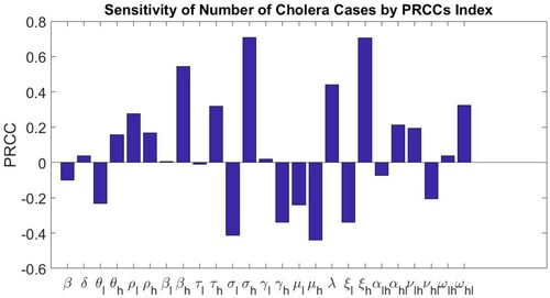
Table 5. Model parameters, corresponding PRCC and corresponding p-values resulting from the sensitivity analysis.
3. Discrete-time risk-structured model with vaccination, treatment and sanitation
As noted in Che et al., cholera intervention strategies such as vaccination, treatment and improved water sanitation have been used to reduce the number of cholera infections. In Cameroon, treatment and water sanitation were first reported in 2004, while vaccination was first reported in 2015 [Citation8,Citation9,Citation11]. In the next section, we introduce these three cholera intervention strategies in Model (Equation4(4)
(4) ).
3.1. Formulation of structured model with vaccination, treatment and sanitation
In Model (Equation4(4)
(4) ), we make the following assumptions in each unit time interval
.
The fractions of high- and low-risk susceptible populations that are vaccinated are
The fractions of susceptible individuals that are vaccinated do not exceed the fractions that do not transition to another risk group. That is,
The fractions of the high- and low-risk infectious populations that receive therapeutic treatment are
The fractions of infectious individuals that receive therapeutic treatment do not exceed the fractions that do not recover from the cholera infection. That is,
The fractions of vibrios in the high and low-risk groups that die due to improved water sanitation are
The fractions of vibrios that die due to improved water sanitation do not exceed the fraction that is not cleared. That is,
Our assumptions and notation lead to the following structured model with vaccination, treatment and sanitation:
(9)
(9) with initial conditions:
and
When there are no cholera interventions and
, then Model (Equation9
(9)
(9) ) reduces to Model (Equation4
(4)
(4) ). Note that Model (Equation4
(4)
(4) ) and Model (Equation9
(9)
(9) ) share the same equation for
, Equation (Equation5
(5)
(5) ). As in the scaling of Model (Equation4
(4)
(4) ), we let
and
for
Also, we let
for
In proportions, Model (Equation9
(9)
(9) ) becomes
(10)
(10) where
and
for
In the next section, we compute , the effective reproduction number for Model (Equation10
(10)
(10) ).
3.2. Discrete-time risk-structured model with vaccination, treatment and sanitation: DFE and
Model (Equation10(10)
(10) ) has a trivial DFE
and a non-trivial DFE
where
and
where
and
For Cameroon,
and the trivial DFE,
, is unstable. For the non-trivial DFE,
, as in the previous section, assuming that
and
are not new infections, we obtain that F, the matrix of new infections, is
where
and T, the matrix of transition terms, is
where
Thus,
, the spectral radius of
, is
(11)
(11) where
implies the DFE,
, is locally asymptotically stable and our intervention strategies have successfully eliminated cholera in Cameroon. However,
implies the DFE,
, is unstable, cholera invades and our intervention strategies have not succeeded in eliminating the disease in Cameroon population.
3.3. Numerical exploration
Pre-intervention Model (Equation6(6)
(6) ) and Model (Equation10
(10)
(10) ) share the common pre-intervention parameter values of Table . As in [Citation5], we use Model (Equation10
(10)
(10) ) to assess the impact of the seven cholera intervention strategies, described in Table , on the number of cholera infections in Cameroon. As in Section 2.4, using scaled values of the actual yearly reported cholera cases (as shown on Figure ) and the multistart algorithm with the fmincon function, we estimated that
(see Table ).
Table 6. Intervention parameters, their descriptions and values.
Table 7. Intervention strategies and their descriptions [Citation5].
From Table , intervention strategies 1, 2 and 3 are single policies of cholera vaccination only, treatment only or improved sanitation only, respectively. However, intervention strategies 4, 5 and 6 are double policies of 1 and 2 only, or 2 and 3 only, or 1 and 3 only, respectively, while intervention strategy 7 is a combination of all the three single policies.
Intervention Strategy 1: The fraction of the low-risk susceptible population that is vaccinated is less than the fraction of high-risk susceptible population that is vaccinated.
Cholera vaccination in Cameroon was first reported in 2015. To illustrate the implementation of strategy 1 only from 2015 to 2019, we let
in Model (Equation10
(10)
(10) ). Figure (a) shows that Model (Equation10
(10)
(10) ) captures the decreasing effect of the vaccination only intervention strategy. Furthermore, Model (Equation10
(10)
(10) ) predicted that in 2019, with vaccination only, the percentage decrease in the number of cholera cases is
. With vaccination only, the effective reproduction number
.
Figure 7. Single Intervention Strategies. (a) Impact of vaccination. , and the number of cholera infections is decreased by
. (b) Impact of treatment.
, and the number of cholera infections is decreased by
. (c) Impact of sanitation.
, and the number of cholera infections is decreased by
.
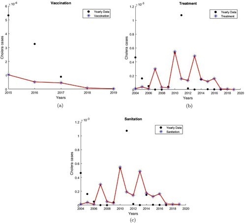
Intervention Strategy 2: The fraction of the low-risk infectious population that is treated is less than the fraction of high-risk infectious population that is treated.
Cholera treatment in Cameroon was first reported in 2004. To illustrate the implementation of strategy 2 only from 2004 to 2019, we let
in Model (Equation10
(10)
(10) ). Figure (b) shows that Model (Equation10
(10)
(10) ) captures the decreasing effect of the treatment only intervention strategy. Furthermore, Model (Equation10
(10)
(10) ) predicted that in 2019, with treatment only, the percentage decrease in the number of cholera cases is
. With treatment only, the effective reproduction number
.
Intervention Strategy 3: The fraction of the pathogen in low risk group that dies due to improved water sanitation is less than the fraction of pathogen in high-risk group that dies due to improved water sanitation.
Improved water sanitation in Cameroon was first reported in 2004. To illustrate the implementation of strategy 3 only from 2004 to 2019, we let
in Model (Equation10
(10)
(10) ). Figure (c) shows that Model (Equation10
(10)
(10) ) captures the decreasing effect of the improved water sanitation only strategy. Furthermore, Model (Equation10
(10)
(10) ) predicted that in 2019, with improved water sanitation only, the percentage decrease in the number of cholera cases is
. With improvement in water sanitation only, the effective reproduction number
.
In Cameroon, with our choice of parameters, none of the single intervention policies reduces to a value below 1. However, as in [Citation5], vaccination only policy decreases the number of cholera cases most and has the lowest single policy
value. Next, we consider dual policies, and the combined policy of all three strategies.
Intervention Strategy 4: The fraction of susceptible individuals that are vaccinated and the fraction of infectious individuals that are treated in the low-risk group are less than the fraction of susceptible individuals that are vaccinated and the fraction of infectious individuals that are treated in the high-risk group, respectively.
To illustrate the implementation of strategy 4 from 2015 to 2019, we let
and
in Model (Equation10
(10)
(10) ). Figure (a) shows that Model (Equation10
(10)
(10) ) captures the decreasing effect of the vaccination and treatment strategy. Furthermore, Model (Equation10
(10)
(10) ) predicted that in 2019, with vaccination and treatment, the percentage decrease in the number of cholera cases is
. With vaccination and treatment, the effective reproduction number
.
Figure 8. Double Intervention Strategies. (a) Impact of vaccination and treatment. , and the number of cholera infections is decreased by
. (b) Impact of treatment and sanitation.
, and the number of cholera infections is decreased by
. (c) Impact of vaccination and sanitation.
, and the number of cholera infections is decreased by
.
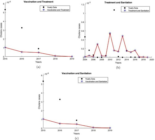
Intervention Strategy 5: The fraction of infectious individuals that are treated and the fraction of pathogen that die due to sanitation in the low-risk group are less than the fraction of infectious individuals that are treated and the fraction of pathogen that die due to sanitation in the high-risk group, respectively.
To illustrate the implementation of strategy 5 from 2004 to 2019, we let
in Model (Equation10
(10)
(10) ). Figure (b) shows that Model (Equation10
(10)
(10) ) captures the decreasing effect of the treatment and sanitation strategy. Furthermore, Model (Equation10
(10)
(10) ) predicted that in 2019, with treatment and improved water sanitation, the percentage decrease in the number of cholera cases is
. With treatment and sanitation, the effective reproduction number
.
Intervention Strategy 6: The fraction of susceptible individuals that are vaccinated and the fraction of pathogen that die due to improved water sanitation in the low-risk group are less than the fraction of susceptible individuals that are vaccinated and the fraction of pathogen that die due to improved water sanitation in the high-risk group,respectively.
To illustrate the implementation of strategy 6 from 2015 to 2019, we let
in Model (Equation10
(10)
(10) ). Figure (c) shows that Model (Equation10
(10)
(10) ) captures the decreasing effect of the vaccination and sanitation strategy. Furthermore, Model (Equation10
(10)
(10) ) predicts that by 2019, with vaccination and improved water sanitation, the percentage decrease in the number of cholera cases is
. With vaccination and sanitation, the effective reproduction number
. As in [Citation5], under the double policy, a vaccination and treatment policy can lead to a highest percentage decrease in the number of cholera cases and the smallest
.
Intervention Strategy 7: The fraction of susceptible individuals that are vaccinated, the fraction of infectious individuals that are treated and the fraction of pathogen that dies due to improved water sanitation in the low-risk group are less than the fraction of susceptible individuals that are vaccinated, the fraction of infectious individuals that are treated and the fraction of pathogen that dies due to improved water sanitation in the high risk group, respectively.
To implement strategy 7 from 2015 to 2019, we let
in Model (Equation10
(10)
(10) ). Figure shows that Model (Equation10
(10)
(10) ) captures the decreasing effect of the combined strategy. Furthermore, Model (Equation10
(10)
(10) ) predicted that in 2019, with the combined strategy, the percentage decrease in the number of cholera cases is
. With this strategy, the effective reproduction number
. Table summarizes estimates of the reproduction numbers and percentage decreases in cholera cases for the 7 different intervention strategies over the periods of intervention.
Figure 9. Impact of vaccination, treatment and sanitation. , and the number of cholera infections is decreased by
.
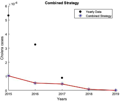
Table 8. Reproduction numbers and percentage decreases in cholera cases for the seven different intervention strategies over the periods of intervention.
In Table , we summarize the corresponding ODE cholera model results from [Citation5]. From Tables and , we see that the ODE and discrete-time cholera intervention strategies results are consistent. However, the discrete-time model predicts a decrease in the number of cholera cases in a shorter period of cholera intervention (2015–2019, see Table ) as compared to the ODE model's period of intervention (2015–2022, see Table ).
Table 9. Reproduction numbers and percentage decreases in cholera cases for the seven different intervention strategies over the periods of intervention [Citation5].
3.4. Sensitivity indices of
As before, we compute the sensitivity indices of with respect to each of the 31 Model (Equation10
(10)
(10) ) parameters, using the baseline parameter values given in Table and that of the estimated intervention parameters in Table (see Table ). From these results, unlike the ODE model in [Citation5], where the most sensitive parameter with the intervention model is
, the recovery rate of infectious individuals in the high-risk group, the most sensitive parameter with our discrete-time intervention model is
, the fraction of low-risk susceptible individuals that are vaccinated. From Table ,
. Thus, decreasing (or increasing)
by
increases (or decreases)
by
. Another important parameter is
, the fraction of susceptible individuals that transition from the low-risk group to the high-risk group. From Table ,
. Thus, decreasing (or increasing)
by
increases (or decreases)
by
. Unlike the ODE model in [Citation5], where the least sensitive parameter is
, the death rate of the cholera pathogen due to improved water sanitation in the low-risk group, the least sensitive parameter in our model with intervention is
, the transmission rate between susceptible individuals and infectious individuals in the high-risk group. From Table ,
. Thus, decreasing (or increasing)
by
decreases (or increases)
by
. Among the six intervention parameters, unlike in [Citation5], where the most sensitive parameter is
, the vaccination rate of susceptible individuals in the high-risk group, and the least sensitive parameter is
, the death rate of the cholera pathogen due to improved water sanitation in the low-risk group, the most sensitive intervention parameter in our discrete-time model is
, the fraction of susceptible individuals in the low-risk group that are vaccinated, and the least sensitive parameter is
, the fraction of the pathogen in the high-risk group that dies due to improved water sanitation.
Table 10. Sensitivity indices of with respect to the 31 parameters for the structured model with intervention, evaluated at the baseline parameter values in Table and that of the estimated intervention parameters in Table .
3.5. Global sensitivity analysis
As before, we perform a global sensitivity analysis for our discrete-time model with an intervention using LHS and PRCC. Now, our number of input parameters is 31 and the number of LHS draws is 80. Table gives the PRCCs and the p-values for each model parameter, while Figure shows the sensitivity of the number of model predicted cholera cases to changes in parameters of Tables and as computed by the LHS-PRCC index. Based on the p-values, we observe that PRCC values for and
are statistically significant. In the ODE model in [Citation5], the parameters
(scaled contact rate between susceptible individuals and cholera pathogen in the high-risk group),
(rate at which recovered individuals become susceptible individuals in the high-risk group) and
(transition rate of recovered individuals from low-risk group to high-risk group) show a significant positive correlation with the total number of model predicted cholera cases. Meanwhile,
and
(the rates at which infectious individuals become recovered individuals in the low and high-risk groups, respectively), λ (the net decay rate of the cholera pathogen) and
(transition rate of recovered individuals from high-risk group to low risk group) show a significant negative correlation with the total number of the ODE model predicted cholera cases. In our discrete-time model,
, the contact rate between susceptible individuals and the cholera pathogen in the low-risk group shows a significant positive correlation with the total number of our discrete-time model predicted cholera cases. On the other hand, λ, the net decay rate of pathogen shows a significant negative correlation with the total number of our discrete-time model predicted cholera cases. This is in agreement with our discrete-time model predictions. That is, increasing
increases the total number of model predicted cholera cases while increasing λ decreases the total number of model predicted cholera cases.
Figure 10. Sensitivity of the number of cholera cases to changes in parameters in Tables and as computed by the Latin Hypercube Sampling-Partial Rank Correlation Coefficient (LHS-PRCC) index.
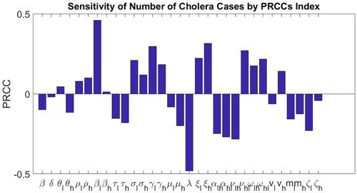
Table 11. Model parameters, corresponding PRCC and corresponding p-values resulting from the sensitivity analysis.
4. Discrete-time model versus the continuous-time ODE model
Both our discrete-time and continuous-time models are Cameroon data-driven parametrized models. However, unlike the continuous-time model, the discrete-time model is based on the discrete-time censoring of the population and cholera data of Cameroon. From Figure , we see that unlike the continuous-time ODE model in [Citation5] that captures the known cholera endemicity in Cameroon with a relative error of 0.8637, with a smaller relative error of 0.8441, our discrete-time risk-structured model also captures the known cholera endemicity in Cameroon. Moreover, unlike the continuous-time ODE model in [Citation5] that predicted a decreasing trend from 1987 to 1994 and an increasing trend from 1995 to 2004 in the pre-intervention reported number of cholera cases in Cameroon from 1987 to 2004, our discrete-time model predicts the observed oscillatory nature in the reported cholera cases in Cameroon.
From our sensitivity analysis, we obtain that, as in the ODE model in [Citation5], in our discrete-time model is not sensitive to changes to the parameters of the demographic equation. For
, unlike the ODE model in [Citation5], where the most sensitive parameter is
, the recovery rate of infectious individuals in the high-risk group, in our discrete-time model, the most sensitive parameter is
, the contact rate between the susceptible individuals and the cholera pathogen in the high-risk group. In [Citation5], the least sensitive parameters are
and
, the parameters associated with loss of immunity, and
and
, transition rates of recovered individuals between the two risk groups. In our discrete-time model, the least sensitive parameters are
and
, the fraction of recovered individuals in the high-risk group who become susceptible, and
and
, the fraction of recovered individuals who transition from the low-risk group to the high-risk group and from the high-risk group to the low-risk groups, respectively. Another important parameter that has a high impact on
in our discrete-time model is
, the fraction of exposed individuals in the high-risk group that can progress to the infectious class. In the ODE model in [Citation5],
, the scaled contact rate between susceptible individuals and the cholera pathogen in the high-risk group shows a significant positive correlation with the total number of cholera cases and
, the recovery rate of infectious individuals in the high-risk group shows a significant negative correlation with the total number of cholera cases. In our discrete-time model,
, the contact rate between susceptible individuals and the cholera pathogen in the high-risk,
, the fraction of exposed individuals that can progress to the infectious class and
, the shedding rate of pathogens by infectious individuals in the high-risk group show a significant positive correlation with the total number of cholera cases.
Under the single intervention policies of vaccination only or treatment only or improved sanitation only, in Table , we obtained that, as in [Citation5], a vaccination only policy has the smallest value of the effective reproduction number and the highest percentage decrease in the number of cholera cases. As in [Citation5], under the double intervention policies of vaccination and treatment only or treatment and improved sanitation only or vaccination and improved sanitation only, in Table we obtained that the double policy of vaccination and treatment has the smallest value for
and the highest percentage decrease in the number of cholera cases. As in [Citation5], each of the three strategies of either vaccination and treatment, or vaccination and improved sanitation, or the combined strategy of vaccination, treatment and improved sanitation is capable of eliminating cholera in Cameroon with the combined strategy having the lowest value for the effective reproduction number,
, and the highest percentage decrease in the number of cholera cases. As in [Citation5], the combined strategy of vaccination, treatment and improved sanitation lead to the smallest number of cholera infections in Cameroon. From Tables and , our discrete-time model results confirm that of the ODE model. However, since the discrete-time model is built on the discrete-time census data it predicts a decrease in the number of cholera cases in a shorter time interval of cholera intervention (2004–2019, see Table ) as compared to the ODE model's time interval of intervention (2004–2022, see Table ).
Again from our sensitivity analysis, we obtain that for , unlike the ODE model in [Citation5], where the most sensitive parameter with the intervention model is
, the recovery rate of infectious individuals in the high-risk group and the least sensitive parameter is
, the death rate of the cholera pathogen due to improved water sanitation in the low-risk group, in our discrete-time model with intervention, the most sensitive parameter is
, the fraction of susceptible individuals in the low-risk group that is vaccinated, while the least sensitive parameter is
, the transmission rate between susceptible individuals and infectious individuals in the high-risk group. Another important parameter is
, the fraction of susceptible individuals that transition from the low-risk group to the high-risk group. Among the six intervention parameters, unlike in [Citation5], where the most sensitive parameter is
, the vaccination rate of susceptible individuals in the high-risk group, and the least sensitive parameter is
, the death rate of the cholera pathogen due to improved water sanitation in the low-risk group, the most sensitive parameter in our discrete-time model is
, the fraction of susceptible individuals in the low-risk group that is vaccinated, and the least sensitive parameter is
, the fraction of the pathogen in the high-risk group that dies due to improved water sanitation.
In the ODE model in [Citation5], the parameters (scaled contact rate between susceptible individuals and cholera pathogen in the low-risk group),
(the rate at which recovered individuals become susceptible individuals in the high-risk group) and
(transition rate of recovered individuals from low-risk group to high-risk group) show a significant positive correlation with the total number of model predicted cholera cases. Meanwhile,
and
(the rates at which infectious individuals become recovered individuals in the low and high-risk groups, respectively), λ (the net decay rate of the cholera pathogen) and
(transition rate of recovered individuals from high-risk group to low-risk group) show a significant negative correlation with the total number of model predicted cholera cases. In our discrete-time model,
, the contact rate between susceptible individuals and the cholera pathogen in the low-risk group shows a significant positive correlation with the total number of our discrete-time model predicted cholera cases. On the other hand, λ, the net decay rate of the pathogen shows a significant negative correlation with the total number of our discrete-time model predicted cholera cases. These global sensitivity results are in agreement with our discrete-time model predictions.
In Table , we summarize the results for our discrete-time model and the continuous-time ODE models. Our results show that both models lead to different results even when they have almost the same . Both models are based on observations and assumptions of the cholera disease dynamics in Cameroon. However, unlike the continuous-time model, the discrete-time model is also based on the observation that the Cameroon data are reported annually (at discrete-time intervals). Thus, the difference equations of the discrete-time model are a closer fit to the observed cholera cases in Cameroon than the ordinary differential equations of the continuous-time cholera model.
Table 12. Results for discrete-time model and continuous-time ODE model.
5. Conclusion
Usually, populations are censored at discrete-time intervals. To capture this discrete censoring of populations in a disease model, we introduce a simple low-high-risk discrete-time structured parametric cholera model of Cameroon with no spatial structure but with direct (human-to-human) and indirect (contaminated water-to-human) infection pathways. We use the discrete-time demographic equation (disease-free equation) to fit the total annual population of Cameroon and then use the fitted discrete-time risk-structured model to capture the reported cholera cases in Cameroon from 1987–2004. In Figure , we obtain that, as in the ODE model in [Citation5], our demographic equation captures the observed exponential population growth of Cameroon. The demographic threshold for the fitted model, . The basic reproduction number for our discrete-time model is
, and that of the ODE cholera model in [Citation5] with a similar risk-structure is 1.1803. Thus, the two models have approximately the same value for
and both predict cholera endemicity in Cameroon. From Figure , unlike the ODE model that predicted a decreasing trend from 1987 to 1994 and an increasing trend from 1995 to 2004 in the pre-intervention reported number of cholera cases in Cameroon from 1987 to 2004, our fitted discrete-time risk-structured cholera model predicts an increasing trend from 1987 to 1989, 1990 to 1992, 1993 to 1995, 1997 to 1998 and 2003 to 2004, and a decreasing trend from 1989 to 1990, 1992 to 1993, 1995 to 1997 and 1998 to 2003, in the pre-intervention reported number of cholera cases in Cameroon from 1987 to 2004.
As in [Citation5], we perform sensitivity analysis to determine the impact of each model parameter on the threshold parameters and
and on the total number of our model's predicted cholera cases. As in the ODE model in [Citation5], we obtained that
is not sensitive to changes to the parameters of the demographic equation. For
, unlike the ODE model in [Citation5], where the most sensitive parameter is
, the recovery rate of infectious individuals in the high-risk group, in our discrete-time model, the most sensitive parameter is
, the contact rate between the susceptible individuals and the cholera pathogen in the high-risk group. In [Citation5], the least sensitive parameters are
and
, the parameters associated with loss of immunity, and
and
, transition rates of recovered individuals between the two risk groups. In our discrete-time model, the least sensitive parameters are
and
, the fraction of recovered individuals in the high-risk group who become susceptible, and
and
, the fraction of recovered individuals who transition from the low-risk group to the high risk group and from the high-risk group to the low-risk groups, respectively. Another important parameter that has a high impact on
in our discrete-time model is
, the fraction of exposed individuals in the high-risk group that can progress to the infectious class. In the ODE model in [Citation5],
, the scaled contact rate between susceptible individuals and the cholera pathogen in the high-risk group shows a significant positive correlation with the total number of cholera cases and
, the recovery rate of infectious individuals in the high risk group shows a significant negative correlation with the total number of cholera cases. In our discrete-time model,
, the contact rate between susceptible individuals and the cholera pathogen in the high risk,
, the fraction of exposed individuals that can progress to the infectious class and
, the shedding rate of pathogens by infectious individuals in the high risk group show a significant positive correlation with the total number of choleracases.
As in [Citation5], using our fitted low-high discrete-time risk-structured cholera model, we study the impact of the following seven cholera intervention strategies on the number of reported cholera cases in Cameroon:
Vaccination only
Treatment only
Improved Sanitation only
Vaccination and Treatment
Treatment and Improved Sanitation
Vaccination and Improved Sanitation
Vaccination, Treatment and Improved Sanitation
From Tables and , our discrete-time model results confirm that of the ODE model. However, since the discrete-time model is built on the discrete-time census data it predicts a decrease in the number of cholera cases in a shorter time interval of cholera intervention (2004–2019, see Table ) as compared to the ODE model's time interval of intervention (2004–2022, see Table ).
We perform sensitivity analysis to determine the impact of each model parameter on the threshold and on the total number of predicted cholera cases by our model with intervention. For
, unlike the ODE model in [Citation5], where the most sensitive parameter with the intervention model is
, the recovery rate of infectious individuals in the high-risk group and the least sensitive parameter is
, the death rate of the cholera pathogen due to improved water sanitation in the low-risk group, in our model the most sensitive parameter in our model is
, the fraction of susceptible individuals in the low-risk group that is vaccinated, while the least sensitive parameter is
, the transmission rate between susceptible individuals and infectious individuals in the high-risk group. Another important parameter is
, the fraction of susceptible individuals that transition from the low-risk group to the high-risk group. Among the six intervention parameters, unlike in [Citation5], where the most sensitive parameter is
, the vaccination rate of susceptible individuals in the high-risk group, and the least sensitive parameter is
, the death rate of the cholera pathogen due to improved water sanitation in the low-risk group, the most sensitive parameter in our discrete-time model is
, the fraction of susceptible individuals in the low-risk group that are vaccinated, and the least sensitive parameter is
, the fraction of the pathogen in the high-risk group that dies due to improved water sanitation.
In the ODE model in [Citation5], the parameters (scaled contact rate between susceptible individuals and cholera pathogen in the low-risk group),
(rate at which recovered individuals become susceptible individuals in the high-risk group) and
(transition rate of recovered individuals from low-risk group to high-risk group) show a significant positive correlation with the total number of model predicted cholera cases. Meanwhile,
and
(the rates at which infectious individuals become recovered individuals in the low and high-risk groups, respectively), λ (the net decay rate of the cholera pathogen) and
(transition rate of recovered individuals from high-risk group to low-risk group) show a significant negative correlation with the total number of model predicted cholera cases. In our discrete-time model,
, the contact rate between susceptible individuals and the cholera pathogen in the low-risk group shows a significant positive correlation with the total number of our discrete-time model predicted cholera cases. On the other hand, λ, the net decay rate of the pathogen shows a significant negative correlation with the total number of our discrete-time model predicted cholera cases. These global sensitivity results are in agreement with our discrete-time model predictions.
Our results show that using ODE and difference equations to model populations that are censored at discrete-time intervals can lead to different results even when the different models have almost the same . Both the continuous-time and discrete-time cholera models of Cameroon are based on observations and assumptions of the cholera disease dynamics in Cameroon. However, unlike the continuous-time model, the discrete-time model is also based on the observation that the cholera cases in Cameroon are reported annually. Thus, the difference equations of our novel discrete-time model are a closer fit to the observed cholera cases in Cameroon than the ordinary differential equations of the continuous-time cholera model. As in [Citation5], our discrete-time models are not spatially structured. When data become available and our model is fully parameterized, a study of a discrete-time spatially structured cholera model with cost analysis of intervention strategies in Cameroon will be an interesting extension of this work.
Acknowledgments
We also appreciate travel awards to support travel expenses from the Society of Industrial and Applied Mathematics, and Biology and Medicine through Mathematics. We thank the anonymous reviewers for a thorough reading and helpful suggestions that improved our exposition.
Disclosure statement
No potential conflict of interest was reported by the author(s).
Additional information
Funding
References
- M. Ali, A.R. Nelson, A.L. Lopez, and D.A. Sack, Updated global burden of cholera in endemic countries, PLoS Negl. Trop Dis. 9(6) (2015), p. e0003832.
- L. Allen and P. van den Driessche, The basic reproduction number in discrete-time epidemic models, J Differ. Equ. Appl 14(10–11) (2008), pp. 1127–1147.
- S.M. Blower and H. Dowlatabadi, Sensitivity and uncertainty analysis of complex models of disease transmission: An HIV model, as an example, Int. Statist. Rev. 62(2) (1994), pp. 229–243.
- F. Brauer, Z. Feng, and C. Castillo-Chavez, Discrete epidemic models, Math. Biosci. Eng. 7(1) (2010), pp. 1–15.
- E. Che, Y. Kang, and A. Yakubu, Risk structured model of cholera infections in Cameroon, Math. Biosci. 320 (2020), p. 108303.
- N. Chitnis, J.M. Hyman, and J.M. Cushing, Determining important parameters in the spread of malaria through the sensitivity analysis of a mathematical model, Bull. Math. Bio. 70(70) (2008), pp. 1272–1296.
- C. Edholm, B. Levy, A. Abebe, T. Marijani, S. Le Fevre, S. Lenhart, A. Yakubu, and F. Nyabadza, A Risk-Structured Mathematical Model of Buruli Ulcer Disease in Ghana, in Mathematics of Planet Earth, H. Kaper, F. Roberts, eds., Mathematics of Planet Earth, Vol. 5, Springer, Cham, 2019.
- Global Citizen, Cameroon: Using vaccines to combat cholera. Available at https://www.globalcitizen.org.
- C.J. Hemmer, J. Nöske, S. Finkbeiner, G. Kundt, and E.C. Reisinger, The cholera epidemic of 2004 in Douala, Cameroon: a lesson learned, Asian Pacific J. Tropical Med. 12(8) (2019), pp. 347–352.
- N. Hernandez-Ceron, Z. Feng, and C. Castillo-Chavez, Discrete epidemic models with arbitrary stage distributions and applications to disease control, Bull. Math. Biol. 75(10) (2013), pp. 1716–1746.
- International Medical Corps, Water Points Transform Cameroonian Villages, Prevent Spread of Cholera. Available at https://internationalmedicalcorps.org.
- S. Marino, I.B. Hogue, C.J. Ray, and D.E. Kirschner, A methodology for performing global uncertainty and sensitivity analysis in systems biology, J. Theoretical Bio. 254(1) (2008), pp. 178–196.
- M. Martcheva, Discrete Epidemic Models, in An Introduction to Mathematical Epidemiology, Texts in Applied Mathematics, Vol 61, Springer, Boston, MA, 2015.
- M.D. McKay, R.J. Beckman, and W.J. Conover, A comparison of three methods for selecting values of input variables in the analysis of output from a computer code, Technometrics 21 (1979), pp. 239–245.
- Political Map of Cameroon. Available at https://www.mapsofworld.com/cameroon/cameroon-political-map.html.
- D. Posny, C. Modnak, and J. Wang, A multigroup model for cholera dynamics and control, Int. J. Biomath. 9(1) (2016), p. 1650001.
- The World Bank, Data, Cameroon. The World Bank. Available at https://data.worldbank.org/country/cameroon?view=chart.
- J.H. Tien and D.J.D. Earn, Multiple transmission pathways and disease dynamics in a waterborne pathogen model, Bull. Math. Biol. 72 (2010), pp. 1502–1533.
- UNICEF, Cholera epidemiology and response factsheet Cameroon. Available at https://www.unicef.org/cholera/files/UNICEF-Factsheet-Cameroon-EN-FINAL.pdf.
- P. van den Driessche, Reproduction numbers of infectious disease models, Infectious Disease Model. 2 (2017), pp. 288–303. https://doi.org/https://doi.org/10.1016/j.idm.2017.06.002.
- P. van den Driessche and A. Yakubu, Demographic population cycles and R0 in discrete-time epidemic models, J. Biol. Dyn. 13(1) (2019), pp. 179–200.
- P. van den Driessche and A. Yakubu, Disease extinction versus persistence in discrete-time epidemic models, Bull. Math. Biol. 81 (2018), pp. 4412–4446. https://doi.org/https://doi.org/10.1007/s11538-018-0426-2.
- J. Wang and C. Modnak, Modeling Cholera dynamics with controls, Canadian Appl. Math. Q. 19(3) (2011), pp. 255–273.
- WHO, https://www.who.int/news-room/fact-sheets/detail/cholera.
- WHO, Weekly Epidemiological Record 92(36) (2017), pp. 521–536. http://www.who.int/wer.
- WHO, https://www.who.int/immunization/diseases/cholera/en/.
- World Health Organization, Global Health Observatory data repository by category, Cholera. Available at http://apps.who.int/gho/data/node.main.174?lang=en.
- A. Yakubu and N. Ziyadi, Discrete-time exploited fish epidemic models, N. Afr. Mat. 22(2) (2011), pp. 177–199.