Chimera and cluster collective states in a dispersal ecological network under state-dependent feedback control and complex habitat structure

Abstract

Pest control based on an economic threshold (ET) can effectively prevent excessive pest control measures such as pesticide abuse and overharvesting. The instinctive dispersal of pest populations in biological network patches for better survival poses challenges for pest management. As long as the pest density is controlled below the economic threshold and no pest outbreak occurs, the aim of pest management can be achieved and it is not necessary to completely remove the pests. This study focuses on the issues of chimera states and cluster solutions in regular bidirectional biological networks with state-dependent impulsive pest management. We consider the influence of two different control modes on the system states, namely global control and local control. Local control is found to be more likely to induce the chimera state. In addition, in the local coupling mode, a higher coupling strength is more likely to generate a coherent state, whereas a lower coupling strength is more likely to generate chimera and incoherent states. Furthermore, the cluster size is inversely related to the coupling strength under local coupling and global control.

Keywords:

• Chimera state
• cluster solution
• dispersal network
• state-dependent feedback control
• integrated pest management

1. Introduction

Integrated pest management (IPM) is defined as an effective pest control approach that usually combines chemical strategies (use of pesticides) with biological strategies (release of natural enemies) as well as other strategies (physical or mechanical control) to keep the pest population at a tolerable level in an ecosystem [2,3,9,11,16,19,29–31]. According to the pest control execution process, pest eradication can be mainly categorized into two types: time-related eradication and state-related eradication. In time-related eradication, pests are eradicated at discrete or fixed time [30,31]. However, even if the pest density is low, pest control measures may continue to be adopted. To prevent such inefficient pest management, in state-related eradication [14,33,35–37,42], only a few control strategies, such as releasing natural enemies, are adopted as long as the pest density does not reach the economic threshold (ET). However, when the pest density exceeds ET, multiple control strategies may be simultaneously adopted to prevent the pest density from reaching the economic injury level (EIL), which is the lowest pest density that will result in economic losses. Note that ET and EIL usually satisfy certain proportions, i.e. $ET\approx 80\mathrm{\%}$ or $85\mathrm{\%}$ EIL [3,20,24,30,34]. IPM is a type of long-term pest management approach that is beneficial for agricultural crops as well as the environment.

Although pests in an ecosystem generally inhabit a relatively fixed region, species often migrate from one region to another for better survival [10,13,40]. The moving behaviour forms a network structure consisting of nodes and edges from the perspective of graph theory, where the nodes are equivalent to patches of the population habitat and the edges indicate whether the population can move between a pair of patches. If there is an edge, the population can move from one patch to another, if there is no edge, the population cannot move directly from one patch to another. The process of population movement is referred to as dispersal. Through dispersal, individuals can move in or out of patches, thereby increasing or decreasing the population density in a certain patch. In many cases, population dispersal is a response to changes in food resources and the environment. Population dispersal is significant in many aspects. First, it can prevent the generation of bad offspring from long-term inbreeding and enable the population to adapt to unsuitable climates or environments. Second, it can expand the population distribution, facilitate the search for a suitable living environment, and prevent the destruction of the entire whole population under extreme local circumstances. Third, it is beneficial for maintaining the stability of the population structure as well as for reducing population pressure and aggressive behaviour. In recent decades, such dispersal ecological networks have attracted considerable attention [10,13,22,40]. For example, Holland and Hastings [13] verified that different dispersal networks (a regular network, a rewired network based on a regular network by replacing m edges at random, and a random network) have a significant impact on the ecological dynamics.

The number of cluster solutions of a regular network is smaller than that of an irregular network and increasing the randomness of the network will increase the size of the cluster solution. A heterogeneous network has a long asynchronous dynamic period, which usually leads to a smaller fluctuation amplitude and a higher risk of population extinction. Marleau et al. [22] highlighted the importance of considering finite-size ecosystems and found that the spatial structure and scale can be predicted on the basis of the eigenvalues and eigenvectors of the connectivity matrix. Guichard and Gouhier [10] investigated the non-equilibrium spatial dynamics of the Rosenzweig–MacArthur predator–prey model, and pointed out that irregular spatiotemporal variability is caused by environmental fluctuations. Asynchronous persistence can be achieved by limited parasitoid movement, and species can avoid extinction by increasing the abundance of local hosts through passive movement from other locations. Yuan et al. [40] studied the complex dynamics of a predator–prey network model for IPM. Cluster solutions can be categorized into two types: solutions with low amplitude fluctuations and solutions with high amplitude fluctuations. This duality contradicts the previous conclusion that heterogeneity in the initial population density generally produces a variety of cluster oscillations.

Population diffusion not only enables the interacting species to generate cluster solutions but also promotes chimera collective behaviour [26]. The chimera phenomenon is a spatiotemporal state in which synchrony and asynchrony can coexist [5–8,17,21,25,27,38,39,41]. Kuramoto and Battogtok [18] were the first researchers to observe the coexistence of coherence and incoherence in coupled oscillators with nonlocal coupling. Subsequently, this intriguing state was definitively designated as a chimera state [1]. In terms of ecological models, Hizanidis et al. [12] discovered that the presence of chimera states can account for different dynamical states, where individuals in some communities exhibit the same phase oscillation, whereas it may be incoherent for those in other communities. Chimera states were also observed in the Rosenzweig–MacArthur network model [4]. By tuning the power-law exponent of the long-range interaction, the coupling topology can be varied among local, nonlocal, and global coupling. The variation of the coupling structure induces transitions between spatial synchrony and various chimera patterns. In [8], collective behaviour among coupled dynamical units was observed in various forms as a result of different coupling topologies as well as different types of coupling functions. It was concluded that chimera states emerge in local, nonlocal, and global coupling topologies, as well as in modular, temporal and multilayer networks. Multicluster and chimera states have been observed as the addition of weighted mean-field dispersal of species to ecological networks with all-to-all connected patches and habitat complexity shrinks the synchrony region and expands the homogeneous steady state region [26]. In an ecological system, the dispersal process often brings spatial synchrony; if one species becomes extinct, all other species will be prone to extinction. Spatially asynchrony has been proven to enhance population persistence stability at a suitable metapopulation scale [28].

In the cluster states, the entire metapopulation is classified as several subgroups based on their synchronization characteristics, and in each subgroup, the patches follow the same synchronous rhythm while these patches are asynchronous among subgroups. In chimera states, the patches are divided into two groups; the patches are completely synchronous in one group, whereas the other patches are asynchronous in another group. In some cases, 1-cluster can be regarded as the coherent state, n-cluster can be regarded as the incoherent state, and 2-cluster to n-1- cluster can be regarded as the chimera states. In terms of pest management, the simultaneous extermination of pests in the patches is regarded as the best result. If such an ideal state cannot be achieved, the pests should be kept below the economic threshold, which is also a desirable result of pest management. Consequently, this study mainly considers the influence of the coupling strength, state-dependent impulse effect, and degree of distribution on the chimera and cluster states of the predator-prey network model, with the objective of providing a theoretical basis for pest management.

2. Mathematical model and preliminaries

2.1. Mathematical model

The classical Holling II predator–prey model was introduced in [32,34]: (1) $\{\begin{array}{l}{\displaystyle {\displaystyle \frac{\mathrm{d}x(t)}{\mathrm{d}t}}=rx(t)[1-{\displaystyle \frac{x(t)}{K}}]-{\displaystyle \frac{\beta x(t)y(t)}{1+\omega x(t)}},}\\ {\displaystyle {\displaystyle \frac{\mathrm{d}y(t)}{\mathrm{d}t}}={\displaystyle \frac{\eta \beta x(t)y(t)}{1+\omega x(t)}}-\delta y(t),}\end{array}$(1) where $x(t)$ represents the prey density (pest) and $y(t)$ denotes the predator density (natural enemy), r and K denote the intrinsic growth rate and the carrying capacity of the prey population, respectively, and $\frac{\eta \beta x(t)y(t)}{1+\omega x(t)}$ is the Holling II functional response, where η, β, and ω are positive constants. Specifically, η represents the rate at which predators digest or transform preys, β denotes the maximum rate at which a predator consumes per unit of prey, ω is the half-saturation constant of the predator population with regard to the prey population, and δ is the death rate of the predator population. Tang et al. proved that system (1(1) $\{\begin{array}{l}{\displaystyle {\displaystyle \frac{\mathrm{d}x(t)}{\mathrm{d}t}}=rx(t)[1-{\displaystyle \frac{x(t)}{K}}]-{\displaystyle \frac{\beta x(t)y(t)}{1+\omega x(t)}},}\\ {\displaystyle {\displaystyle \frac{\mathrm{d}y(t)}{\mathrm{d}t}}={\displaystyle \frac{\eta \beta x(t)y(t)}{1+\omega x(t)}}-\delta y(t),}\end{array}$(1) ) always has an unstable steady state $(0,0)$, a stable or unstable boundary equilibrium $(K,0)$, and a positive steady state $E^{\ast }=(\frac{\delta }{\eta \beta -\delta \omega },\frac{r\eta (K\eta \beta -K\delta \omega -\delta )}{K{(\eta \beta -\delta \omega )}^2})$. By incorporating an economic threshold in system (1(1) $\{\begin{array}{l}{\displaystyle {\displaystyle \frac{\mathrm{d}x(t)}{\mathrm{d}t}}=rx(t)[1-{\displaystyle \frac{x(t)}{K}}]-{\displaystyle \frac{\beta x(t)y(t)}{1+\omega x(t)}},}\\ {\displaystyle {\displaystyle \frac{\mathrm{d}y(t)}{\mathrm{d}t}}={\displaystyle \frac{\eta \beta x(t)y(t)}{1+\omega x(t)}}-\delta y(t),}\end{array}$(1) ), the predator–prey model can be rewritten as a state-dependent impulsive semi-dynamic system: (2) $\{\begin{array}{rl}& \begin{array}{l}{\displaystyle \frac{\mathrm{d}x(t)}{\mathrm{d}t}=rx(t)[1-\frac{x(t)}{K}]-\frac{\beta x(t)y(t)}{1+\omega x(t)},}\\ {\displaystyle \frac{\mathrm{d}y(t)}{\mathrm{d}t}=\frac{\eta \beta x(t)y(t)}{1+\omega x(t)}-\delta y(t),}\end{array}\}x(t)<\mathit{\text{ET}},\\ & \begin{array}{l}x(t^{+})=qx(t),\\ y(t^{+})=y(t)+\tau ,\end{array}\}x(t)=ET,\end{array}$(2) where ET is the economic threshold and $q\in [0,1)$ is the remaining proportion of pests removed by control measures such as spraying pesticides, artificial capture, or the release of natural enemies once the pest density reaches ET. Here, τ is the number of natural enemies released at time t. Further, by extending the predator–prey system with state-dependent feedback control to dispersal coupled networks, the following structure is considered in this study: (3) $\{\begin{array}{rl}& \begin{array}{l}{\displaystyle \frac{\mathrm{d}{x}_i(t)}{\mathrm{d}t}=r{x}_i(t)[1-\frac{x_i(t)}{K}]-\frac{\beta x_i(t)y_i(t)}{1+\omega x_i(t)}+\sum _{j=1}^N{x}_j{d}_{x_{ij}}{a}_{ij},}\\ {\displaystyle \frac{\mathrm{d}{y}_i(t)}{\mathrm{d}t}=\frac{\eta \beta x_i(t)y_i(t)}{1+\omega x_i(t)}-\delta y_i(t)+\sum _{j=1}^N{y}_j{d}_{y_{ij}}{a}_{ij},}\end{array}\}{x}_i(t)<ET,\\ & \begin{array}{l}{x}_i(t^{+})=q_i{x}_i(t),\\ y_i(t^{+})=y_i(t)+{\tau }_i,\end{array}\}{x}_i(t)=ET,\end{array}$(3) where $d_{x_{ij}}$ ($d_{y_{ij}}$) is the dispersal rate of the species from patch i to patch j $(i=1,2,\dots ,N;j=1,2,\dots ,N)$, $x_i(t)$ and $y_i(t)$ are the prey and predator densities of the ith patch, respectively. The number of patches for each species in the network is N. System (3(3) $\{\begin{array}{rl}& \begin{array}{l}{\displaystyle \frac{\mathrm{d}{x}_i(t)}{\mathrm{d}t}=r{x}_i(t)[1-\frac{x_i(t)}{K}]-\frac{\beta x_i(t)y_i(t)}{1+\omega x_i(t)}+\sum _{j=1}^N{x}_j{d}_{x_{ij}}{a}_{ij},}\\ {\displaystyle \frac{\mathrm{d}{y}_i(t)}{\mathrm{d}t}=\frac{\eta \beta x_i(t)y_i(t)}{1+\omega x_i(t)}-\delta y_i(t)+\sum _{j=1}^N{y}_j{d}_{y_{ij}}{a}_{ij},}\end{array}\}{x}_i(t)<ET,\\ & \begin{array}{l}{x}_i(t^{+})=q_i{x}_i(t),\\ y_i(t^{+})=y_i(t)+{\tau }_i,\end{array}\}{x}_i(t)=ET,\end{array}$(3) ) includes $2N$ coupled ordinary differential equations. Further, $a_{ij}$ is the matrix representing the permitted dispersal transitions, and $C\equiv a_{ij}=A-E$, where A is the adjacency matrix of the dispersal network. If $A_{ij}=1$, then the individuals can move from patch j to patch i. The diagonal matrix E denotes emigration, and $E_{ii}=\sum _{j=1}^N{A}_{ji}$ [13]. In this study, we assume that the two populations only flow within the system, i.e. no immigrants enter the system, and no emigrants leave the system. Note that $d_{x_{ij}}=d_{y_{ij}}=c$, $q_i=q$, and ${\tau }_i=\tau$ are also assumed. In terms of biological significance, if the pest density reaches the economic threshold, IPM is required to reduce the pest density and increase the number of natural enemies; thus, $0\le q<1$, $\tau >0$.

2.2. Preliminaries

2.2.1. Network types

Researchers have developed a variety of Internet, social and biological networks in recent years [23]. According to the direction between the network nodes (patches), networks can be categorized into two types: undirected networks (see Figure 1(a–c)) and directed networks (see Figure 1(d–f)). In Figure 1, each network has 10 patches, which are marked as $1,2,\dots ,10$. Figure 1(a,d) shows the two types of networks of degree 4. We use them to represent locally coupled networks. Figure 1(b,e) shows two random networks. The edges in these networks are randomly connected and the probability is 0.1. Figure 1(c,f) shows two networks of degree 9, which are called fully connected or globally coupled networks. Because the connection structure of each node is identical, the networks in Figure 1(a,c,d,f) are all regular networks.

Figure 1. (Colour online) Two types of networks for 10 nodes. (a,b,c) Undirected networks; (d,e,f) directed networks.

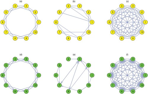
Different network structures are distinguished according to different connectivities, which can be determined by the adjacency matrix A. It has been verified that the connectivity of two populations can be depicted among various patches by coupled networks, with the two species migrating freely between a pair of connected patches [40]. Regular networks with different degrees based on a ring network are investigated in this study. In ecological networks, the nodes are also known as patches and the undirected network is bidirectional, which means that the species can move freely between two patches.

2.2.2. Standard deviation ${\sigma }_{\overline{CL}}$ for chimera measure

To investigate the effects of the coupling strength c and impulsive equation parameter q of system (3(3) $\{\begin{array}{rl}& \begin{array}{l}{\displaystyle \frac{\mathrm{d}{x}_i(t)}{\mathrm{d}t}=r{x}_i(t)[1-\frac{x_i(t)}{K}]-\frac{\beta x_i(t)y_i(t)}{1+\omega x_i(t)}+\sum _{j=1}^N{x}_j{d}_{x_{ij}}{a}_{ij},}\\ {\displaystyle \frac{\mathrm{d}{y}_i(t)}{\mathrm{d}t}=\frac{\eta \beta x_i(t)y_i(t)}{1+\omega x_i(t)}-\delta y_i(t)+\sum _{j=1}^N{y}_j{d}_{y_{ij}}{a}_{ij},}\end{array}\}{x}_i(t)<ET,\\ & \begin{array}{l}{x}_i(t^{+})=q_i{x}_i(t),\\ y_i(t^{+})=y_i(t)+{\tau }_i,\end{array}\}{x}_i(t)=ET,\end{array}$(3) ) on its dynamical behaviours, the standard deviation ${\sigma }_{\overline{CL}}$ is considered: (4) ${\sigma }_{\overline{CL}}={\left(\frac{1}{N}\sum _{i=1}^N{(C{L}_i-\overline{CL})}^2\right)}^{\frac{1}{2}},$(4) where $\overline{CL}$ is the mean value of the pulse interval (PI) for all the patches, which is given by (5) $\overline{CL}=\frac{1}{N}\sum _{i=1}^{N}C{L}_i.$(5) $C{L}_i$ is the coefficient of variation, (6) $C{L}_i=\frac{{\sigma }_{P{I}_i}}{\overline{P{I}_i}},$(6) where $P{I}_i$ is the time difference between two pulses, i.e. the time difference between the two instances in which the prey density of patch i reaches ET. $\overline{P{I}_i}$ is the mean value of $P{I}_i$ and ${\sigma }_{P{I}_i}$ is the standard deviation of $P{I}_i$.

According to the definition of ${\sigma }_{\overline{CL}}$, the closer $C{L}_i$ and $\overline{CL}$ are, the closer is ${\sigma }_{\overline{CL}}$ to zero. When ${\sigma }_{\overline{CL}}=0$, the oscillation patterns of all the patches are identical. This is known as the coherent state. Otherwise, the chimera state or incoherent state is generated.

2.2.3. Linear pairwise correlation coefficients ${\rho }_{ij}$ for cluster solution

Linear pairwise correlation coefficients are used to distinguish the different chimera dynamics [15]. These coefficients are given by (7) ${\rho }_{ij}=\frac{\sum _{i=1}^N\sum _{j=1}^N(x_i-{\overline{x}}_i)(x_j-{\overline{x}}_j)(y_i-{\overline{y}}_i)(y_j-{\overline{y}}_j)}{{(\sum _{i=1}^N{(x_i-{\overline{x}}_i)}^2{(y_i-{\overline{y}}_i)}^2)}^{\frac{1}{2}}{(\sum _{j=1}^N{(x_j-{\overline{x}}_j)}^2{(y_j-{\overline{y}}_j)}^2)}^{\frac{1}{2}}},$(7) where $x_i$, $x_j$ and $y_i$, $y_j$ are the time series of the two populations (i.e. prey and predator); their mean values are given by $\overline{x_i}$, $\overline{x_j}$ and $\overline{y_i}$, $\overline{y_j}$. Note that when $|{\rho }_{ij}|\approx 1$, two patches are considered to be linearly correlated. Thus, when $|{\rho }_{ij}|>0.99$, a ‘population cluster’ can be defined [40]. For instance, if the oscillation patterns of all the patches are identical (globally synchronous), this is the 1-cluster solution. If the oscillation patterns of all the patches are distinct (globally asynchronous), this is referred to as the N-cluster solution (the total number of patches is denoted by N). Solutions of 2-cluster to k-cluster of synchronous patches are defined similarly.

3. Spatiotemporal dynamics

3.1. Chimera state

Chimera states are spatiotemporal patterns characterized by the coexistence of coherent and incoherent domains. Multichimera states or clustered chimera imply that multiple domains of incoherence and coherence exist. In this subsection, incoherent, chimera and coherent states for system (3(3) $\{\begin{array}{rl}& \begin{array}{l}{\displaystyle \frac{\mathrm{d}{x}_i(t)}{\mathrm{d}t}=r{x}_i(t)[1-\frac{x_i(t)}{K}]-\frac{\beta x_i(t)y_i(t)}{1+\omega x_i(t)}+\sum _{j=1}^N{x}_j{d}_{x_{ij}}{a}_{ij},}\\ {\displaystyle \frac{\mathrm{d}{y}_i(t)}{\mathrm{d}t}=\frac{\eta \beta x_i(t)y_i(t)}{1+\omega x_i(t)}-\delta y_i(t)+\sum _{j=1}^N{y}_j{d}_{y_{ij}}{a}_{ij},}\end{array}\}{x}_i(t)<ET,\\ & \begin{array}{l}{x}_i(t^{+})=q_i{x}_i(t),\\ y_i(t^{+})=y_i(t)+{\tau }_i,\end{array}\}{x}_i(t)=ET,\end{array}$(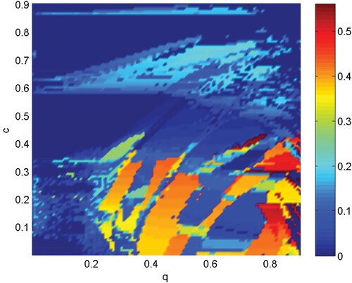3) ) are shown by different colours of parameter space q−c in Figure 2. If ${\sigma }_{\overline{CL}}$ (colour bar) is equal to zero, it indicates that the system stays in the coherent state, which means that every patch has the same oscillation pattern. The incoherent groups are marked in red. Incoherent states imply out-of-phase oscillations close to a limit cycle in the 2N-dimensional state-space or the existence of a chaotic attractor. The chimera state is a transient state between the incoherent state and the coherent state. The transitions from and to the chimera state are mediated by bifurcations, and the chimera is highly sensitive to the initial conditions. Note that the integration time of the numerical procedures employed in the simulations is fixed in the interval [0,320] and the initial values are pseudo-random numbers, where $x_i\in (1,2)$ and $y_i\in (2,3)$. When the coupling strength is high (such as $c\in (0.4,0.9)$), the coherent region occupies a large proportion. A high coupling strength indicates that the population moves between patches with high frequency and quantity. When the coupling strength is low (such as $c\in (0,0.4)$ ), there are more incoherent regions and chimera regions; in this scenario, the remaining proportion parameter q in system (3(3) $\{\begin{array}{rl}& \begin{array}{l}{\displaystyle \frac{\mathrm{d}{x}_i(t)}{\mathrm{d}t}=r{x}_i(t)[1-\frac{x_i(t)}{K}]-\frac{\beta x_i(t)y_i(t)}{1+\omega x_i(t)}+\sum _{j=1}^N{x}_j{d}_{x_{ij}}{a}_{ij},}\\ {\displaystyle \frac{\mathrm{d}{y}_i(t)}{\mathrm{d}t}=\frac{\eta \beta x_i(t)y_i(t)}{1+\omega x_i(t)}-\delta y_i(t)+\sum _{j=1}^N{y}_j{d}_{y_{ij}}{a}_{ij},}\end{array}\}{x}_i(t)<ET,\\ & \begin{array}{l}{x}_i(t^{+})=q_i{x}_i(t),\\ y_i(t^{+})=y_i(t)+{\tau }_i,\end{array}\}{x}_i(t)=ET,\end{array}$(3) ) plays an important role in system state switching.

Figure 2. (Colour online) System states for parameter space q−c, where q is the remaining proportion after removing some pests, and c is the coupling strength (the degree of 10-node network is 4). The colour bar represents the standard deviation ${\sigma }_{\overline{CV}}$; the value ranges from 0 to 0.5601. ${\sigma }_{\overline{CV}}=0$ represents the coherent state, the larger the value of ${\sigma }_{\overline{CV}}$, the more incoherent is the state in which the system tends to be. The other parameters are fixed: r = 2, K = 100, $\beta =0.2$, w = 0.1, $\eta =0.85$, $\delta =0.79$, $\tau =5.5$, and $ET=50$.

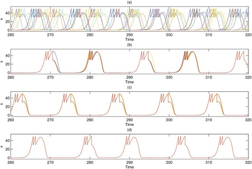
To verify the occurrence of the complex dynamics within this system, spatiotemporal diagrams for a 10-patch ring network of degree 4 are shown in Figure 3. We choose three different sets of parameters and adopt two pest control strategies. One strategy is to control all the patches when the density of pests reaches the ET. The other strategy is to control only some patches (such as odd patches) while the other patches are not controlled (i.e. no pulse control). As can be seen from Figure 3(a–c), three different states are observed under global control (controlling all the patches). The system is in a coherent state for q = 0.4 and c = 0.2 (Figure 3(a)). Adjust the parameters as q = 0.5 and c = 0.8, Figure 3(b) shows the chimera state where incoherent domains are comparatively subtle. The incoherent state can emerge in Figure 3(c) if we fix q = 0.5 and the coupling strength c decreases sharply to 0.001. We are also interested in the results of partial control, i.e. pest control strategies involving odd-numbered patches when the pest population density approach ET. Although Figure 3(d–f) have the same parameters as Figure 3(a–c), the system only generates chimera states different from the three states under global control. This result is attributed to the synchronization of controlled patches and the asynchrony of uncontrolled patches. Therefore, it is difficult for partial control to achieve global synchronization but it is more likely to produce the chimera state.

Figure 3. (Colour online) Spatiotemporal plots for 10-patch ring network of degree 4 under global control and local control. r = 2, K = 100, $\beta =0.2$, w = 0.1, $\eta =0.85$, $\delta =0.79$, $\tau =5.5$ and ET = 50. (a) q = 0.4, c = 0.2, global control, coherent state; (b) q = 0.5, c = 0.8, global control, chimera state (less incoherent areas); (c) q = 0.5, c = 0.001, global control, incoherent state; (d) q = 0.4, c = 0.2, local control, chimera state; (e) q = 0.5, c = 0.8, local control, chimera state; (f) q = 0.5, c = 0.001, local control, chimera state.

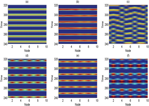
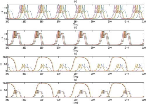
To further demonstrate and distinguish the various states of Figures 3, 4(a–f) presents time series for the pest population $x_i$ of every patch i in the network system corresponding to Figure 3(a–f). As shown in Figure 4(a), the oscillation patterns of the prey population in every patch are completely synchronous, where only the red curve is plotted. Meanwhile, the density of pests reaches ET twice in a period, which means that IPM should be carried out twice. The prey populations of each patch i have their respective oscillation patterns, shown by the 10 different coloured curves in Figure 4(c), which is consistent with the spatial-temporal diagram in Figure 3(c). As the time series curves of the synchronized patches coincide with each other while the curves of asynchronous patches are represented by several different coloured curves, the chimera states observed in Figure 3(b,d–f) are confirmed by Figure 4(b,d–f). Compared with Figures 4(a)–(c) and 4(d–f), we find that under partial control, the number of pests in uncontrolled patches can exceed the preset ET and an outbreak may occur. Thus, in terms of pest control, global control is verified to be better than local control and the effect of partial control is restricted. In addition, when the coupling strength c = 0, from Figure 5, it can be seen that it is difficult for the system to achieve a coherent state in the case of no coupling, regardless of whether it is under global control or local control, more incoherent regions exist. The time series for the pest population of every patch with global or local control corresponding to Figure 5 is shown in Figure 6. When the system is uncoupled, it is easier to produce incoherent and chimera states, whereas it is difficult to achieve a coherent state. When q is fixed, we should release natural enemies and spray insecticides among patches with the same intensity to control the pests. Compared with local control, global control can ensure that the density of pests is always below the ET in order to prevent economic losses.

Figure 4. (Colour online) Time series for the pest population $x_i$ of each patch i ($i=1,2,\dots ,10$) in the ring network corresponding to Figure 3(a–f). (a) q = 0.4, c = 0.2, global control, coherent state; (b) q = 0.5, c = 0.8, global control, chimera state; (c) q = 0.5, c = 0.001, global control, incoherent state; (d) q = 0.4, c = 0.2, local control, chimera state; (e) q = 0.5, c = 0.8, local control, chimera state; (f) q = 0.5, c = 0.001, local control, chimera state. The other parameters are the same as those in Figure 3.

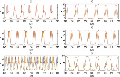
Figure 5. (Colour online) Spatiotemporal plots for 10-patch ring network of degree 4 when coupling strength c = 0. The coupling strength c = 0, and the other parameters are identical to those in Figure 3. r = 2, K = 100, $\beta =0.2$, w = 0.1, $\eta =0.85$, $\delta =0.79$, $\tau =5.5,$ and ET = 50. (a) q = 0.4, c = 0, global control, chimera state; (b) q = 0.5, c = 0, global control, chimera state; (c) q = 0.4, c = 0, local control, chimera state; (d) q = 0.5, c = 0, local control, chimera state.

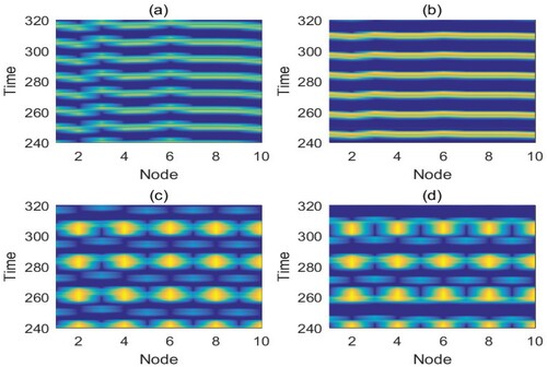
Figure 6. (Colour online) Time series for the pest population $x_i$ ($i=1,2,\dots ,10$) of each patch i in the ring network corresponding to Figure 5. The coupling strength c = 0, and the other parameters are identical to those in Figure 5. r = 2, K = 100, $\beta =0.2$, $w=0.1$, $\eta =0.85$, $\delta =0.79$, $\tau =5.5,$ and ET = 50. (a) q = 0.4, c = 0, global control, chimera state; (b) q = 0.5, c = 0, global control, chimera state; (c) q = 0.4, c = 0, local control, chimera state; (d) q = 0.5, c = 0, local control, chimera state.

3.2. Cluster solutions

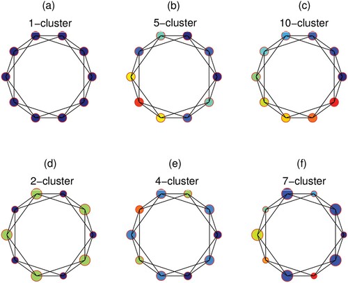
In this subsection, we focus on the effects of the control mode, coupling strength and degree of distribution on the cluster size of the system. According to the definition of the correlation coefficients ${\rho }_{ij}$, patches are considered to belong to the same cluster and possess identical dynamics when the correlation coefficient is close to 1. The spatial arrangement of the patches in the cluster solutions is shown in Figure 7, where patches with identical fluctuation are denoted by circular nodes of the same colour. For example, when all the patches are under global control, 1-cluster, 5-cluster, and 10-cluster solutions are generated (see Figure 7(a–c)). However, with the same parameters, if the patches are under local control, 2-cluster, 4-cluster, and 7-cluster solutions are generated (see Figure 7(d–f)), where the radius of the controlled nodes is smaller than that of the uncontrolled patches. In particular, the 1-cluster solution represents the coherent state through the clustering mechanism while the 10-cluster solution forms the incoherent state. Regardless of whether the nodes are under global control or local control, the cluster size does not necessarily decrease as the coupling strength increases, whereas it reaches the minimum value when the coupling strength is appropriate. Comparing Figures 7(b) and 7(e) with 7(c) and 7(f), we can conclude that global control does not necessarily result in a smaller cluster size faster than local control. When the parameters are the same, local control can sometimes achieve smaller cluster solutions than global control. If we need a smaller cluster solution, local control can sometimes achieve the effect of global control; thus, less time and resources would be required for the pest control of some patches.

Figure 7. (Colour online) Cluster solutions for ring networks of degree 4. The parameters are the same as those in Figure 3. (a) q = 0.4, c = 0.2, global control, 1-cluster; (b) q = 0.5, c = 0.8, global control, 5-cluster; (c) q = 0.5, c = 0.001, global control, 10-cluster; (d) q = 0.4, c = 0.2, local control, 2-cluster; (e) q = 0.5, c = 0.8, local control, 4-cluster; (f) q = 0.5, c = 0.001, local control, 7-cluster; global control: all circular nodes are controlled; local control: smaller circular nodes in (d), (e), (f) are controlled, i.e. part of the nodes are controlled.

However, when we fix q = 0.6 instead of varying it as shown in Figure 7 and set the node degree to 4, the cluster size is inversely related to the coupling strength, i.e. a higher coupling strength c produces fewer cluster solutions. 10-cluster, 6-cluster, 5-cluster, and 1-cluster solutions are identified in Figure 8(a–d) when c = 0.01, c = 0.1, c = 0.2, c = 0.8636, respectively. These solutions correspond to the incoherent state, chimera states, and coherent state, see Figure 8(e–h). The corresponding phase diagrams in Figure 8(i–l) are composed of coincident or non-coincident irregular limit cycles. Together with Figure 9, it is demonstrated that the pest density of each patch experiences periodic fluctuation; the maximum value cannot exceed ET and the minimum value is close to zero (i.e. extinction). Comparing the time series of Figures 6 and 9, we find that as the value of q increases, the actions become more impulsive; in other words, more cycles of pest management are required, which is logical as the number of pests killed each time is small and the pest control frequency is higher.

Figure 8. (Colour online) (a–d) The spatial arrangement of the patches in the cluster solutions for ring networks of degree 4. (e–h) The corresponding spatiotemporal diagrams. (i–l) The corresponding phase diagrams. The coupling strength c from left to right in each column is 0.01, 0.1, 0.2, and 0.8636; q is fixed as 0.6; the other parameters are r = 2, K = 100, $\beta =0.2$, w = 0.1, $\eta =0.85$, $\delta =0.79$, $\tau =5.5$, and ET = 50.

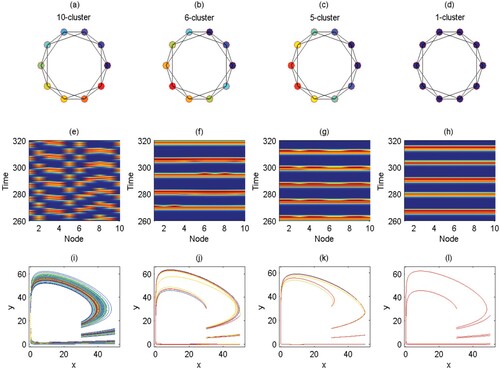
Figure 9. (Colour online) Time series for the pest population $x_i$ ($i=1,2,\dots ,10$) of each patch i corresponding to Figure 8. (a) q = 0.6, c = 0.01, 10-cluster; (b) q = 0.6, c = 0.1, 6-cluster; (c) q = 0.6, c = 0.2, 5-cluster; (d) q = 0.6, c = 0.8636, 1-cluster; the other parameters are r = 2, K = 100, $\beta =0.2$, w = 0.1, $\eta =0.85$, $\delta =0.79$, $\tau =5.5$, and ET = 50.

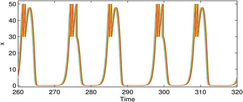
Furthermore, the influence of different coupling strengths on the cluster solutions of the dispersal network of degree 9 is shown in Figure 10. The corresponding time series diagrams are shown in Figure 11. From Figures 10 and 11, the cluster solution and coupling strength are neither in direct proportion nor in inverse proportion when the degree value is 9. The relationship between the cluster solution and the coupling strength is more complex. It seems unreasonable that when the coupling strength is low (c = 0.06365), the system can still produce a smaller 2-cluster solution on account of the large degree value (10 nodes, degree 9). Next, we consider an extreme case in which the coupling strength q = 0. Figure 12 shows the time series for the pest population of each patch in ring networks with degree 4, 6 and 9. Although the degrees are different, because the coupling strength is equal to 0, the time series graphs for the three degrees are identical, as there is no population exchange between patches.

Figure 10. (Colour online) (a–d) The spatial arrangement of the patches in the cluster solutions for ring networks of degree 9. (e–h) The corresponding spatiotemporal diagrams. (i–l) The corresponding phase diagrams. The coupling strength c from left to right in each column is 0.0005, 0.8818, 0.06365, 0.65; q is fixed as 0.6 and the other parameters are fixed as r = 2, K = 100, $\beta =0.2$, w = 0.1, $\eta =0.85$, $\delta =0.79$, $\tau =5.5$, and ET = 50.

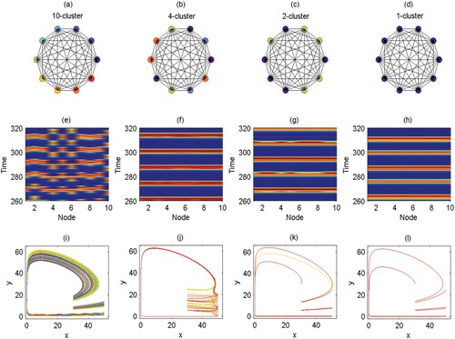
Figure 11. (Colour online) Time series for the pest population $x_i$ ($i=1,2,\dots ,10$) of each patch i corresponding to Figure 10. (a) q = 0.6, c = 0.0005, 10-cluster; (b) q = 0.6, c = 0.8818, 4-cluster; (c) q = 0.6, c = 0.06365, 2-cluster; (d) q = 0.6, c = 0.65, 1-cluster; the other parameters are fixed as $r=2,K=100,\beta =0.2,w=0.1,\eta =0.85,\delta =0.79,\tau =5.5$, and ET = 50.

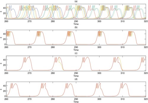
Figure 12. (Colour online) Time series for the pest population $x_i$ ($i=1,2,\dots ,10$) of each patch i with coupling strength c = 0 in the ring networks of degree 4, 6 and 9. q = 0.6, and the other parameters are r = 2, K = 100, $\beta =0.2$, w = 0.1, $\eta =0.85$, $\delta =0.79$, $\tau =5.5$, and ET = 50.

4. Conclusion

Pest management has undergone a transition from fixed time to variable time and further to state-dependent impulse management. In state-dependent impulsive control, pest control measures are adopted according to the system state variables such as pest density. As long as the ET is not reached, the number of pests is allowed to fluctuate in a certain range. Based on IPM, this study focused on a predator–prey dispersal network model with state-dependent feedback control. We investigated the chimera states and cluster solutions of the system in the case of bidirectional regular networks. Under local coupling and global control, the higher the coupling strength, the more obvious is the coherent trend of the network patches. By contrast, the lower the coupling strength, the higher is the probability of incoherent and chimera states. The parameter q plays a crucial role in the transition of system states. Thus, in the case of local coupling, in order to reach the coherent state as soon as possible, the populations must move frequently between patches. In addition to the coupling strength, we also considered the influence of global control (controlling all the network nodes) and local control (controlling odd network nodes) on the system states. With the same parameters, global control can produce three states of incoherence, chimera, and coherence, whereas local control can obtain only the chimera state. We found that it is difficult for the uncontrolled nodes to synchronize with the controlled nodes, and the pest populations in the uncontrolled patches present a periodic outbreakpattern.

For the network model, when the coupling strength is high, the number of clusters is often small, which is mainly due to the diffusion effect of the network. This diffusion effect drives the network nodes toward synchronization. However, in this study, regardless of global control or local control, the cluster size did not necessarily take a smaller value when the coupling strength was high, whereas it reached a smaller value when the coupling strength was appropriate. This is because the impulse effect changes the trajectory of the system, thereby affecting the cluster solution. In addition, the rate of decrease in the cluster size under global control was not higher than that under local control. In the case of local coupling (degree 4), the cluster size decreased as the coupling strength increased. In the case of global coupling (degree 9), the cluster size did not decrease as the coupling strength increased. Furthermore, we verified that when the coupling strength is zero, different degrees of the network nodes have the same influence on the systemstate.

Disclosure statement

No potential conflict of interest was reported by the author(s).

Additional information

Funding

This work was supported in part by the National Natural Science Foundation of China [grant numbers 11961024, 12026233 and 12026221], in part by Youth Project of Scientific and Technological Research Program of Chongqing Education Commission [grant number KJQN201901203], in part by Chongqing higher education reform research project [grant numbers 203443, 203447], in part by the Special Funds for ‘Double First-Class’ Construction in Hubei Province, and in part by Enshi State Science and Technology Planning Project [grant number ZZD19021].

References

- D.M. Abrams and S.H. Strogatz, Chimera states for coupled oscillators, Phys. Rev. Lett. 93 (2004), doi:https://doi.org/10.1103/PhysRevLett.93.174102.
- O. Akman, T.D. Comar, and D. Hrozencik, Model selection for integrated pest management with stochasticity, J. Theor. Biol. 442 (2017), pp. 110–122.
- O. Akman, T. Comar, and M. Henderson, An analysis of an impulsive stage structured integrated pest management model with refuge effect, Chaos Solitons Fractals. 111 (2018), pp. 44–54.
- T. Banerjee, P.S. Dutta, A. Zakharova, and E. Schöll, Chimera patterns induced by distance-dependent power-law coupling in ecological networks, Phys. Rev. E. 94 (2016), p. 032206.
- B.K. Bera and D. Ghosh, Chimera states in purely local delay-coupled oscillators, Phys. Rev. E. 93 (2016), p. 052223.
- B. Bera, D. Ghosh, and M. Lakshmanan, Chimera states in bursting neurons, Phys. Rev. E 93 (2016), p. 012205.
- B. Bera, D. Ghosh, and T. Banerjee, Imperfect traveling chimera states induced by local synaptic gradient coupling, Phys. Rev. E. 94 (2016), p. 012215.
- B.K. Bera, S. Majhi, D. Ghosh, and M. Perc, Chimera states: Effects of different coupling topologies, Europhys. Lett. 118 (2017), p. 10001.
- L.H. Blommers, Integrated pest management in European apple orchards, Annu. Rev. Entomol. 39 (1994), pp. 213–241.
- F. Guichard and T.C. Gouhier, Non-equilibrium spatial dynamics of ecosystems, Math. Biosci. 255 (2014), pp. 1–10.
- L.G. Higley and L.P. Pedigo, Economic Thresholds for Integrated Pest Management. University of Nebraska Press, 1996.
- J. Hizanidis, E. Panagakou, I. Omelchenko, E. Schöll, P. Hövel, and A. Provata, Chimera states in population dynamics: Networks with fragmented and hierarchical connectivities, Phys. Rev. E. 92 (2015), p. 012915.
- M.D. Holland and A. Hastings, Strong effect of dispersal network structure on ecological dynamics, Nature. 456 (2008), pp. 792–794.
- G. Jiang, Q. Lu, and L. Qian, Complex dynamics of a Holling type ii prey–predator system with state feedback control, Chaos Solitons Fractals. 31 (2007), pp. 448–461.
- F.P. Kemeth, S.W. Haugland, L. Schmidt, I.G. Kevrekidis, and K. Krischer, A classification scheme for chimera states, Chaos 26 (2016), p. 094815.
- M. Kogan, Integrated pest management: Historical perspectives and contemporary developments, Annu. Rev. Entomol. 43 (1998), pp. 243–270.
- S. Kundu, B. Bera, D. Ghosh, and M. Lakshmanan, Chimera patterns in three-dimensional locally coupled systems, Phys. Rev. E. 99 (2019), p. 022204.
- Y. Kuramoto and D. Battogtokh, Coexistence of coherence and incoherence in nonlocally coupled phase oscillators: A soluble case, preprint (2002). Available at arXiv:0210694.
- J.V. Lenteren and J. Woets, Biological and integrated pest control in greenhouses., Annu. Rev. Entomol. 33 (1988), pp. 239–269.
- L. Liu, C. Xiang, G. Tang, and Y. Fu, Sliding dynamics of a Filippov forest-pest model with threshold policy control, Complexity 2019 (2019), pp. 1–17.
- S. Majhi, B.K. Bera, D. Ghosh, and M. Perc, Chimera states in neuronal networks: A review, Phys. Life Rev. 28 (2019), pp. 100–121.
- J.N. Marleau, F. Guichard, and M. Loreau, Meta-ecosystem dynamics and functioning on finite spatial networks, Proc. R. Soc. B 281 (2014), p. 20132094.
- M.E. Newman, The structure and function of complex networks, SIAM Rev. 45 (2003), pp. 167–256.
- L. Nie, Z. Teng, L. Hu, and J. Peng, Existence and stability of periodic solution of a predator–prey model with state-dependent impulsive effects, Math. Comput. Simul. 79 (2009), pp. 2122–2134.
- I. Omelchenko, Y. Maistrenko, P. Hövel, and E. Schöll, Loss of coherence in dynamical networks: Spatial chaos and chimera states, Phys. Rev. Lett. 106 (2011), p. 234102.
- S. Saha, N. Bairagi, and S.K. Dana, Chimera states in ecological network under weighted mean-field dispersal of species, Front. Appl. Math. Stat. 5 (2019), p. 00015.
- I.A. Shepelev and T.E. Vadivasova, External localized harmonic influence on an incoherence cluster of chimera states, Chaos Solitons Fractals. 133 (2020), p. 109642.
- C.F. Steiner, R.D. Stockwell, V. Kalaimani, and Z. Aqel, Population synchrony and stability in environmentally forced metacommunities, Oikos 122 (2013), pp. 1195–1206.
- S. Tang and L. Chen, Modelling and analysis of integrated pest management strategy, Discrete Contin. Dyn. Syst. B. 4 (2004), pp. 759–768.
- S. Tang, Y. Xiao, and R.A. Cheke, Multiple attractors of host-parasitoid models with integrated pest management strategies: Eradication, persistence and outbreak, Theor. Popul. Biol. 73 (2008), pp. 181–197.
- S. Tang, J. Liang, Y. Tan, and R.A. Cheke, Threshold conditions for integrated pest management models with pesticides that have residual effects, J. Math. Biol. 66 (2013), pp. 1–35.
- G. Tang, S. Tang, and R.A. Cheke, Global analysis of a Holling type II predator–prey model with a constant prey refuge, Nonlinear Dyn. 76 (2014), pp. 635–647.
- S. Tang, W. Pang, R.A. Cheke, and J. Wu, Global dynamics of a state-dependent feedback control system, Adv. Differ. Equ. 2015 (2015), pp. 322–391.
- S. Tang, B. Tang, A. Wang, and Y. Xiao, Holling II predator–prey impulsive semi-dynamic model with complex Poincare map, Nonlinear Dyn. 81 (2015), pp. 1575–1596.
- S. Tang, C. Li, B. Tang, and X. Wang, Global dynamics of a nonlinear state-dependent feedback control ecological model with a multiple-hump discrete map, Commun. Nonlinear Sci. Numer. Simul.79 (2019), p. 104900.
- Y. Tian, K. Sun, and L. Chen, Modelling and qualitative analysis of a predator–prey system with state-dependent impulsive effects, Math. Comput. Simul. 82 (2011), pp. 318–331.
- Y. Tian, S. Tang, and R.A. Cheke, Nonlinear state-dependent feedback control of a pest-natural enemy system, Nonlinear Dyn. 94 (2018), pp. 2243–2263.
- M. Wildie and M. Shanahan, Metastability and chimera states in modular delay and pulse-coupled oscillator networks, Chaos 22 (2012), p. 043131.
- M. Yi and C. Yao, A chimera oscillatory state in a globally delay-coupled oscillator network, Complexity 2020 (2020), pp. 1–11.
- B. Yuan, S. Tang, and R.A. Cheke, Duality in phase space and complex dynamics of an integrated pest management network model, Int. J. Bifurc. Chaos 25 (2015), p. 1550103.
- F. Zahra, A. Zahra, P. Fatemeh, J. Sajad, P. Matjaz, and S. Mitja, Effects of different initial conditions on the emergence of chimera states, Chaos Solitons Fractals. 114 (2018), pp. 306–311.
- T. Zhang, W. Ma, X. Meng, and T. Zhang, Periodic solution of a prey–predator model with nonlinear state feedback control, Appl. Math. Comput. 266 (2015), pp. 95–107.