Homogenous mixing and network approximations in discrete-time formulation of a SIRS model

Abstract

A discrete-time deterministic epidemic model is proposed to better understand the contagious dynamics and the behaviour observed in the incidence of real infectious diseases. For this purpose, we analyse a SIRS model both in a random-mixing approach and in a small-world network formulation. The models include the basic parameters that characterize an epidemic: infection and recovery times, as well as mechanisms of contagion. Depending on the parameters, the random-mixing model has different types of behaviour of an epidemic: pathogen extinction; endemic infection; sustained oscillations and dynamic extinction. Spatial effects are included in our network-based approach, where each individual of a population is represented by a node of a small-world network. Our network-based approach includes rewiring connections to account for time-varying network structure, a consequence of the natural response to the emergence of an epidemic (e.g. avoiding contacts with infected individuals). Random and adaptive rewiring conditions are analysed and numerical simulation are made. A comparison of model predictions with the actual effects of COVID-19 infection on population that occurred in Italy and France is produced. Results of the time series of infected people show that our adaptive evolving networks represent effective strategies able to decrease the epidemic spreading.

KEYWORDS:

• SIRS epidemics
• temporal networks
• adaptive networks
• epidemiology

1. Introduction

The world population can be severely impacted from the emergence and spread of novel pathogens (as recently with COVID-19), or from a sudden change in the epidemiology of an existing pathogen. Mathematical methods are widely used for understanding mechanisms in the spread of pandemic infectious diseases. A classical mathematical approach is generally based on the SIRS models [1], wherein the host population is partitioned into categories containing susceptible (S), infectious (I) and recovered (R) individuals. The SIRS model applies to diseases against which, as a result of mutation pathogen, individuals lose immunity.

Generally, the transmission dynamics of an infectious disease is described by modelling the population movements among those epidemiological compartments, and assuming random-mixing interactions. When the population mixes at random, each individual has a small and equal chance of coming into contact with any other individual. Over the years, numerous approaches have been proposed. As a result, it is found that SIRS models have endemic asymptotically stable equilibria or an epidemic free equilibrium. In the deterministic framework, periodic solutions exist if the transmission rate is allowed to vary seasonally or spatial heterogeneity is included [11,17]. It is also suggested that non-linear incidence rate [16], temporary immunity (through which an individual’s return to susceptibility can be delayed) [8,4], the introduction of a quarantine class [9], are mechanisms that can induce oscillations in the occurrence of diseases. Periodic epidemic outbreaks can also be observed by properly modelling the transmission rate and the loss of immunity [20]. In the time-delay approach [6], individuals spend a fixed amount of time in a generalized immune class, and oscillations occur for specific ranges of immunity duration and infected individual exposure. When irregular behaviour is added to an oscillatory one, simulation patterns appear to behave in a qualitatively similar fashion to the real diseases (e.g. influenza) [21]. The results of these studies emphasize the importance of well understanding how the nature of the transition between the three different population classes affects the dynamics of an epidemic. To this end, in this paper we generalize the random-mixing approach of Girvan et al. [6] to include different values for the pathogen infection time.

In practice, the number of contacts each individual has is considerably smaller than the population size, as individuals tend to make contact with family members, work colleagues and friends. Therefore, social structure has an important impact on transmission dynamics.

The effects of the social structure on the evolution of epidemics can be described via networks modelling [12,5,31,33]. In fact, a second classical approach describes spatially extended populations such as elements in a network, whose nodes represent individuals and edges stand for interactions among them. Models that incorporate network structure avoid the random-mixing assumption by assigning to each individual a finite set of permanent contacts with people who share social life with them. In these papers, static networks are used to describe the spread of epidemics.

In real epidemiological networks, however, human movement has the consequence that contacts between individuals depend on time, and infectious disease propagation proceeds with concomitant changes in the underlying network structure, because of social network dynamics. Furthermore, individuals may change their behaviour over time in order to avoid infection. In fact, in the presence of an epidemics, both individual and collective reactions can significantly alter the social network structure: non-infected individuals may start avoiding contact with infected ones. Thus, the network structure can change as the connections between susceptible and infective individuals break and new edges are eventually formed with other individuals.

Based on these observations, and in contrast to the models based on static networks, a class of models based on temporal or adaptive networks has been introduced, and the effects of switching social contact have been investigated. The mean-field approaches provide a general theoretical picture of the behaviour of the SIS model in networks. The epidemic dynamics on adaptive or temporal networks is typically studied as an SIS (or SIR) model [2,7,10,15,26–28,32]. Also, a mean-field theory for a recurrent SIRS model on uncorrelated network is studied in [19], and an SIRS model on adaptive network is studied in [25], where mean field equations for the network dynamics are introduced. It is found that disease avoidance strategies can cause both the endemic and extinct states to be bi-stable [7,25]. All these theoretical studies of epidemic spreading rely mostly on the mean-field theory approaches for the node evolution [23].

In this paper, we investigate a different approach using a small-world network representation as introduced by Watts and Strogatz [29]. Small-world networks can be highly clustered, like regular lattices, yet have small characteristic path lengths, like random graphs. Their name derives from Milgram’s ‘six degrees of separation’ experiment [18]. A random procedure allows to interpolate between regular and random networks. Many biological, technological and social networks lie somewhere between these two extremes. In particular, infectious diseases spread more easily in small-world networks than in regular lattices. Our goal is to better understand epidemic processes and predict their behaviour [24].

We consider a small-world network, where a temporal variation of links between nodes is introduced. We follow the small word networks approach (that interpolates between an ordered finite-dimensional lattice and a random graph) [12], where, for a finite value of the disorder of the network (ranging from ordered lattices to random graphs), a transition from a stationary state (fixed point, with fluctuations) to self-sustained oscillations in the size of the infected population was found. In particular, we consider a double temporal variation of the network: one in which susceptible and partly infectious and recovered move randomly on the network (temporal network); another in which the susceptible statistically avoid contact with infected individuals (adaptive network). These random movements are carried out keeping the 2 K coordination number constant (the coordination number 2 K is the average number of links per node, that is the average degree).

We follow the evolution of each node through the various stages of the epidemic, as a more realistic model, rather than linking their dynamics according to a mean field model. Our formulation has the advantage of containing explicitly two significant parameters that characterize an epidemic: the incubation time and the immunity period.

In a preliminary phase, we consider a random-mixing SIRS approach, which includes both loss of immunity and infectious time steps (Section 2). We show that even a traditional mean-field model contains many interesting epidemic features. In Section 3 spatial effects are introduced within a small world network formulation. Simulations on a random temporal network are discussed in Section 4, while social distancing behaviour on an adaptive network is introduced in Section 5, where a comparison with epidemic data of COVID-19 infection in Italy and France is also performed. Conclusions are drawn in Section 6.

2. A random-mixing approach

We consider a population consisting of susceptible (S), infected (I) and recovered (R) individuals. As a consequence, the total population is $N=S_t+I_t+R_t$, and there are no births or deaths (i.e. N is constant).

Susceptible elements can move to the infected state through contagion by an infected one. Conversely infected elements can move to the recovered state, and recovered elements can return to the susceptible state by loss of immunity. This framework is usually referred to as SIRS, from the cycle that each element goes through. The contagion is possible only during the S phase, and only by an I element. During the R phase, the elements are immune and not infectious.

Upon infection, individuals spend${\tau }_I$time steps in the infective class, and the subsequent ${\tau }_R$ time steps in the immune class. After these ${\tau }_0={\tau }_I+{\tau }_R$ time steps, individuals return to the susceptible class.

At any given time step t, the population that is infected can be determined by adding to the infected individuals the fraction that has been infected in any of the previous ${\tau }_I-1$ time steps. The population that is immune at any given time t, can be determined by examining the fraction that has been infected in any of the previous time steps from $t-{\tau }_I$ to $t-{\tau }_0+1$. If at each time step, the I_t ${\text{I}}_{\text{t}}$ infected individuals make $\mu$ random exposures (contact rate), the probability of exposure is $q_t=1-e^{-\mu I_t/N}$ (in the large system limit$N\to \mathrm{\infty }$).

The dynamical system is described by the equations (1) $\begin{array}{rl}{i}_{t+1}& =q_t{S}_t\\ S_{t+1}& =(1-q_t)S_t+i_{t-{\tau }_0+1}\\ I_{t+1}& =\sum _{k=0}^{{\tau }_I-1}{i}_{t-k+1}\\ R_{t+1}& =\sum _{k={\tau }_I}^{{\tau }_0-1}{i}_{t-k+1}\end{array}$(1) where $i_t$ represents the individuals that are infected at each time t, and $i_{t-t_0}$ the individuals that, once infected, return to the susceptible state after a complete cycle $t_0$.

The equations above are redundant, since at each time step $S_t+I_t+R_t=N$. Without loss of generality in this section, we could set N=1. So $S_t$, $l_t$ and $R_t$ are standing for the fraction of individuals in each class (or represent the probability of being in each class).

In addition, the fraction of infected can be calculated explicitly. In fact, an individual is susceptible if it is simply neither infected nor immune, (2) $S_t=1-\sum _{k=0}^{{\tau }_I-1}{i}_{t-k}-\sum _{k={\tau }_I}^{{\tau }_0-1}{i}_{t-k}$(2)

This yields (3) $i_{t+1}=\left(1-e^{-\mu {\sum }_{k=0}^{{\tau }_I-1}{i}_{t-k}}\right)\left(1-\sum _{k=0}^{{\tau }_I-1}{i}_{t-k}-\sum _{k={\tau }_I}^{{\tau }_0-1}{i}_{t-k}\right)$(3)

This model constitutes a generalization of that proposed by Girvan et al. [6], where the particular case ${\tau }_I=1$ was considered. Depending on the parameters, this model has different types of behaviour: (i) pathogen extinction due to lack of contact between individuals; (ii) endemic infection, that is the average number of infected individuals became constant; (iii) the disease persists with sustained oscillations; and (iv) dynamic extinction of the epidemic.

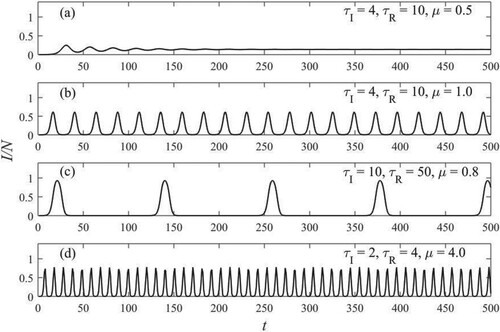
Figure 1 shows numerical iterations of I_t (Equation (1)) starting from the initial conditions $I_t=0$ for $t=1\dots {\tau }_0-1$ and $I_{{\tau }_0}={10}^{-4}$, for different values of the parameters $\mu$, ${\tau }_I$ and ${\tau }_R$ (reported in the insets of figure). Three different patterns of epidemic are represented: non-zero equilibrium [Figure 1(a)], sustained oscillations [Figure 1(b,c)], and quasiperiodic oscillations [Figure 1(d)].

Figure 1. Fraction of infected population versus time. Parameters are in the inset of figures. (a) $I_t$ relaxes to a fixed point. Oscillations of period (b) $T=24$ and (c) $T=120$. (d) Quasiperiodic oscillations.

The fixed points of Equation (3) satisfy (4) $i^{\ast }=(1-e^{-\mu {\tau }_I{i}^{\ast }})(1-{\tau }_0{i}^{\ast })$(4)

Linearizing the exponential about $i^{\ast }$ we obtain (5) $i^{\ast }\cong \mu {\tau }_I{i}^{\ast }(1-{\tau }_0{i}^{\ast })$(5)

The trivial solution $i^{\ast }=0$ always exists and is the only solution if the infection rate $\mu =0$. For $i^{\ast }\ne 0$ we obtain (6) $i^{\ast }\cong \frac{\mu {\tau }_I-1}{\mu {\tau }_I{\tau }_0}$(6) and because $i^{\ast }$ is positive, a stable non trivial fixed point is obtained only for $\mu \stackrel{>}{\sim \phantom{{}_x}}1/{\tau }_I$.

In Figure 2, the phase diagram of the different dynamical behaviours of infected people $I_t$ is shown, for a fixed value of the parameter ${\tau }_I=4$. The curve represents the location of the transitions between the trivial equilibrium, the non-zero steady state and oscillations. The curves that mark the transitions are generated numerically. The boundaries between the different dynamical behaviours are the same also for other values of ${\tau }_I$.

Figure 2. The boundary between persistence and extinction. Hopf and extinction curves are generated numerically.

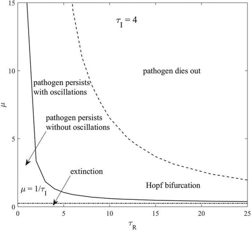
For fixed values of ${\tau }_I$ and ${\tau }_R$, the stability of the fixed points is determined by the parameter $\mu$. When $\mu \stackrel{<}{\sim \phantom{{}_x}}1/{\tau }_I$, $I_t$ approaches the trivial zero solution. As $\mu$ is increased through $1/{\tau }_I$, below the Hopf curve, the non-zero equilibrium becomes an attractor. Increasing $\mu$ through the Hopf curve the fixed point loses stability and the periodic or quasiperiodic orbits emerge. As $\mu$ is further increased the oscillations grow in amplitude, and the fraction of infected individuals $I_t$ gets so low that dynamical extinction occurs due to the population’s finite size. The boundaries between the different types of behaviour follow an inverse relation between contact rate $\mu$ and immunity duration ${\tau }_R$.

The oscillatory behaviours are qualitatively similar to epidemic diseases such as influenza. The period of the oscillations ranges between slightly larger values of ${\tau }_0$ to values approximately equal to $2{\tau }_0$. Once we fix the value of the parameters ${\tau }_I$ and ${\tau }_R$, it is almost always possible to find a range of $\mu$ where dynamical oscillations occur. For low values of $\mu$ susceptible peoples remain large and oscillations do not occur. For high values of $\mu$, large amplitude oscillations produce a number of infected so small that epidemic dies out. We observe from Figure 2 that the wide region of pathogen persistence resides at small values of ${\tau }_R$ and large values of $\mu$. Such a circumstance corresponds to a population with high contact rate and a pathogen that gives short period of immunity.

3. Epidemic model on a small-world network

The random-mixing approach can be easily generalized to include spatial effects. Each individual of the population is represented by a node of a small-world network described by one of the three stages, S, I and R. Interactions between elements of the population are described by the network connections, and infection can propagate through them. We take a ring lattice of N vertices and coordination number 2 K (node degree). Each edge is then rewired at random, with probability $p$, to any vertex of the system, and preserved with probability $1-p$. Self connections and multiple connections are prohibited.

The parameter $p$ controls the randomness of the resulting network, i.e. the transition between a regular lattice ($p=0$) and a random graph ($p=1$), by rewiring each edge at random with probability p. As $p$ increases, the clustering is maintained up to quite large values of $p$, while the short average path lengths already appear for quite modest values of $p$. As a result, there is a substantial range of intermediate values for which the model shows both effects simultaneously.

Each element i of the network is characterized by a time counter ${\tau }_i=0,1,\dots ,{\tau }_I+{\tau }_R\equiv {\tau }_0$ describing the phase of disease. A susceptible element S stays at ${\tau }_i=0$ until it can become infected if connected to infected individuals. Once infected (I), in the first ${\tau }_I$ time step it can potentially transmit the disease to its susceptible neighbours. In the following ${\tau }_R$ steps it remains in state R, where it is not contagious and also immune to disease. The cycle is completed after these ${\tau }_0$ time steps, when it return to the susceptible state [12].

The contagion of a susceptible by infected elements occur stochastically at a local level. If a susceptible element $i$ has $k_i$ neighbours, of which $k_{\text{inf}}$ are infected, then it will become infected with probability ${\mu }_{k_i}=k_{\text{inf}}/k_i$ (in the following we use also ${\mu }_{k_i}=\lambda k_{\text{inf}}/k_i$, where a node becomes infected with probability $\lambda$ if all of its neighbors are infected). This choice is not the only possible one. If we assume that a susceptible has a probability $0<\lambda \le 1$ of contagion with each infected neighbour, the probability that the individual is not infected is simply $(1-\lambda {)}^{k_{\text{inf}}}$ and the probability of infection is ${\mu }_{k_i}=1-(1-\lambda {)}^{k_{\text{inf}}}$. Nonetheless, we note that for values of λ ≤ 0.2 both these criteria give qualitatively the same results [12]. We use the first choice for the infection probability, which is the most frequently used in the literature [5,12,31].

We have performed numerical simulations on networks with the number of nodes ranging from $N={10}^3$ to ${10}^5$, with $K=3$. An initial fraction of infected nodes $I_0/N=0.1$, with the rest in susceptible state, was used almost everywhere. If the network is considered static, no individuals can change their links. This means that a population in which social contacts remain unchanged over time it is treated. Generally, in this case evolution over time of the fraction of infected individuals shows a different pattern as the disorder parameter changes: for low values of $p$ the stationary state is a fixed point with fluctuations; at high values of $p$ large amplitude, self-sustained oscillations develop [12]. In some cases, their amplitude is great enough to produce the infection of almost the whole population and after the period of immunity the infection could end at a fixed time $t$, with no further evolution. Unlike what stated in [12] (where, for large p only regular oscillations were observed), we found in the space of parameter $[{\tau }_I,{\tau }_{\text{R}}]$ regions where, although $p$ was large or $p=1$, the time series has irregular behaviour. This can happen for small values of ${\tau }_0$ (see Section 5).

4. Numerical simulations on a random temporal network

As social contacts can change over time, in real epidemiological networks the infectious propagation follows changes in the underlying network. To incorporate human behaviour in the dynamics of epidemic spread, we rewire the network during infectious disease propagation. The movements of people are regulated by the parameter $n_{\text{rew}}$, which determines the number of links rewired at each time step.

Rewiring is done by randomly taking two edges $n_{\text{rew}}$ times and exchanging randomly their links, and it is carried out keeping the 2 K coordination number constant.

We show in Figure 3 part of four time series of density of the infected nodes for different values of the disorder parameter $p$ and of the rewiring parameter $n_{\text{rew}}$. The curves correspond to systems with $N=5\cdot {10}^3$, $K=3$, ${\tau }_I=4$, ${\tau }_R=9$. For a static network ($n_{\text{rew}}=0$), at low values of the disorder parameter ($p=0.01$), the stationary state is a fixed point, with fluctuations [Figure 3(a)]. This case resembles to that of an endemic infection, with a low and recurrent fraction of infected people. In fact, the endemic infection describes a disease that is present at an approximately constant level in a region or population. For large values of the disorder parameter [Figure 3(d)], large amplitude self-sustained oscillations develop. Those are found to exist in many real epidemics. The oscillations are almost periodic with small fluctuation in amplitude. The time series of Figure 3(d) has a period $T=20$. This behaviour at $p=1$ resembles that of the mean field model [see Figure 1(d)].

Figure 3. Fraction of infected elements as a function of time, corresponding to different values of the disorder parameter $p$ and the rewiring parameter $n_{\text{rew}}$, as shown in the legends. Other parameters are $N=5\cdot {10}^3$, $K=3$, ${\tau }_I=4$, ${\tau }_R=9$, $I_0/N=0.1$.

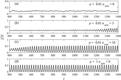
The curves in Figure 3(b) and 3(c) represent the state of the system at $p=0.01$, where $n_{\text{rew}}=3$ and $n_{\text{rew}}=10$ edge per time step are rewired. It is clearly seen that, as time has increased and the contemporary rewind has taken place, the fluctuations in the time series are attenuated and regular oscillations of increasing amplitude appear [Figure 3(b)]. This effect is even more evident in Figure 3(c), where at about $t>700$ the oscillations assume an amplitude equal to that seen in the time series of Figure 3(d), where $p=1$ and no rewiring was carried out. 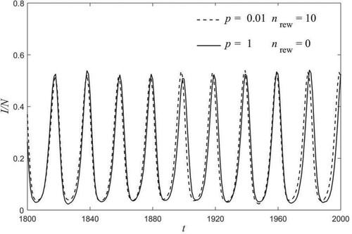For larger values of $t$ the curves are practically equal and in phase, as can be clearly seen in Figure 4.

Figure 4. Comparison between time series of infected nodes at p = 0.01 and n_rew = 10 (dashed line) with p = 1 and n_rew = 0 (solid line). Other parameters are as in Figure 3.

The formation of persistent oscillations on a static network corresponds to a spontaneous synchronization of a significant fraction of the elements in the system. Although the homogeneous mixing model of Section 2 predicts the presence of oscillations, it is capable of describing the dynamics of the network only at $p=1$, without being able to provide explanations at lower values of the parameter that regulates the disorder. Conversely, in a dynamic network this effect is attributed to the lower clustering due to large values of $p$ [12]. In practice, when $p$ is small, if an infected node is in a cluster, it remains there until the deterministic cycle was completed (except in cases where ${\tau }_0$ is large [5]). Rewinding increases the network disorder and has the consequence of gradually driving the system toward synchronization, smoothing out irregularities and gradually increasing the amplitude of the oscillations, until a state similar to that of a random network is reached.

Thus, the information that a given node is infected spreads faster, because the population is moving. This sharing of contacts leads to collective phenomena like oscillating excitations appearing spontaneously in the system.

5. Epidemic dynamics on an adaptive network

Humans tend to respond to the emergence of an epidemic by avoiding contacts with infected individuals, via social distancing or externally imposed policy interventions. The effect of avoiding infection is accounted for by eliminating existing connections and creating new ones (Figure 5). Such rewiring of the local connections can have a strong effect on the dynamics of the disease, which in turn influences the rewiring process. Thus, a mutual interaction between a time varying network topology and the dynamics of the nodes emerges.

Figure 5. Rules of the adaptive network model describing disease spread. (a) A susceptible individual becomes infected with probability ${\mu }_{k_i}=k_{\text{inf}}/k_i$, stays a time ${\tau }_I$ in the class I, then a time ${\tau }_R$ in the recovered class R, before returning to susceptible state. In an adaptive network, (b) two links I-S can change (rewire) to I-I and S-S or (c) links I-S and I-S (or R) in can change (rewire) to I-I and S-S (or R), in order to avoiding the infection.

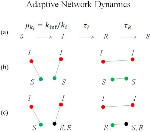
When there are contacts between S and I, to avoid the disease the contacts between people are selectively rewired, replacing them with contacts between S and S (or R). In our model, an S-I (i.e. between a susceptible and an infected) edge is randomly sampled. Therefore, a second edge is chosen randomly from those not connected to the previous one. It is observed if this second edge connects an infected and an uninfected node (S-I) (case (b), later marked with the initials SS) or an infected and recovered node (R-I) (case (c) later marked with the initials SR). This condition is sought for at least 100 times. If this condition becomes true, these two edges are finally changed so as to connect the two infected nodes to each other (I-I, and the remaining two between non-infected, S-S or S-R). Double connections and self-connections are not allowed to form. At each time step this procedure is repeated $n_{\text{rew}}$ times, keeping the connectivity 2 K constant.

The dynamical evolution of the system is the consequence of the competition between the rate of infection and the amount of human interactions breaking. At each time step, a new number of infections occur, part of the infected recovers, and part of recovered becomes susceptible. At the same time, a number of $n_{\text{rew}}$ pairs of infected nodes disconnect from susceptible nodes and connect to each other, and similarly makes the pairs of susceptible disconnected. If the breaking of connections is slow relative to the timescale of the pathogen, the dynamical behaviour is induced basically by the network structure $p$ (rewiring increases $p$) and the infection features (${\tau }_I$, ${\tau }_R$). Conversely, when the breaking of infectious links is large, infected peoples are mostly connected between them, as if they were confined, and epidemic can break off.

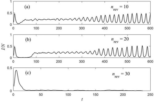
This behaviour is illustrated in Figure 6, where the fraction of infected peoples versus time is shown for three different values of $n_{\text{rew}}$. In Figure 6(a) after an initial outbreak and an irregular steady-state value, a low amplitude periodic pattern in a background of fluctuations is observed, then the time series converge to oscillatory behaviour (with a mean value around $I/N\cong 0.21$). The same happens in Figure 6(b), with the difference that after the outbreak there is a time interval ($25\stackrel{<}{\sim \phantom{{}_x}}t\stackrel{<}{\sim \phantom{{}_x}}65$), where the fraction of infected people has a very low steady state value ($I/N\cong 0.08$). In both cases, avoiding infection has only the effect of postponing the oscillatory behaviour at large values of $t$. When rewiring is sufficiently high [$n_{\text{rew}}=30$ in Figure 6(c)], the adaptive behaviour is predominant. After the outbreak, infection decays toward a steady-state behaviour (at $t\cong 22$) surrounded by stochastic noise.

Figure 6. Fraction of population infected versus the number of time steps for different values of $n_{\text{rew}}$, as shown in the legends. Other parameters are $N=2\cdot {10}^3$, $K=3$, ${\tau }_I=4$, ${\tau }_R=9$, $p=0.01$, $I_0/N=0.1$. Dynamics evolve on an adaptive network as described in Figure 5(b).

The behavioural adaptations and the consequent confinement of infected individuals drastically lowers the intensity of the epidemic. The latter however remains active due to the new susceptible nodes that come from a recovered state and are subject to being infected again. The system stays for a long time in the state that corresponds to that of an endemic infection, with a low and persistent fraction of infected individuals (on average $I/N=0.0021$). The epidemic ends when the last confined infective nodes become immune (here at $t=235$). The reason why the infection continues to sustain itself for a long time, at a minimum value, is due to adaptive rewiring of SS, stricter with respect to the choice of SR. However, this is not always the case, as dynamics are also determined by random processes.

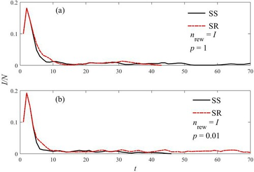
This aspect is clearly exemplified in Figure 7, where the epidemic ends at t = 92 and t = 39 for the SS and SR cases, respectively.

Figure 7. Fraction of infected versus time. The plots refer to the different rules of rewiring shown in Figure 5. Parameters are as in Figure 6, with the exception of n_rew = 60.

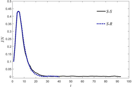
Figure 8. Fraction of infected people for ${\tau }_I=2$, ${\tau }_R=4$, $N=2\cdot {10}^3$, $K=3$, $I_0/N=0.1$. (a) For p = 1, dynamics shows irregular behaviour both for n_rew = 0 (dotted curve). At $n_{\text{rew}}=60$, rewiring keeps well under control the epidemics both for SR (dashed curve) and SS rule (solid curve). (b) For $p=0.01$ clustering alone is adequate to control the spread of the epidemics. Rewiring with both SR and SS rules the infection ends before.

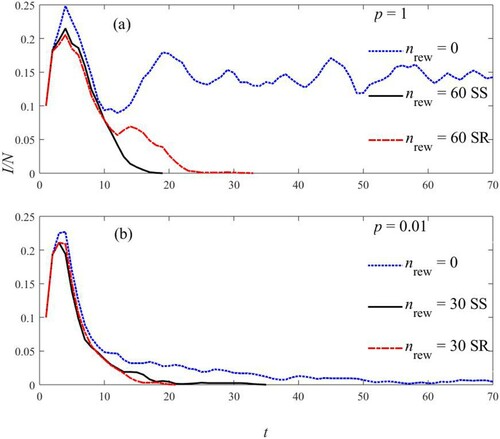
The time step where the epidemic fade out depends greatly on the relative values of ${\tau }_I$, ${\tau }_R$ and $p$. In Figure 8(a) (dotted line) we show an example for ${\tau }_I=2$, ${\tau }_R=4$ of non-typical behaviour of the system, as mentioned at end of Section 3. We observe in the figure that even for $p=1$ there is no regular oscillation, and a pattern of small amplitude oscillations is mixed with a background of high fluctuations. To quantify the synchronization behaviour, we can use the order parameter [12] (7) $\sigma (t)=\left|\frac{1}{N}\sum _{j=1}^N{e}^{i{\phi }_j(t)}\right|$(7) where ${\varphi }_j=2\pi ({\tau }_j-1)/{\tau }_0$ is a geometrical phase corresponding to ${\tau }_j$. The state $\tau =0$ have been left out in the sum in Equation (7). We find, averaging over 10 realizations, the value $\sigma =0.42$, according to the observed temporal pattern.

Even with $n_{\text{rew}}=30$ this behaviour remains unchanged (not shown in the figure), with only a lowering of the mean value of $I$ (for $n_{\text{rew}}=0$, $I/N=0.142$; for $n_{\text{rew}}=30$, $I/N=0.119$ for SS rewiring and $I/N=0.124$ for SR rewiring). $n_{\text{rew}}=60$ must be reached to find the control of rewiring over to infection, which ends at $t=19$ for SS and a $t=33$ for SR rewiring, respectively [Figure 8(b)].

The situation is different for $p=0.01$, where the network is highly clustered. This prevents that the epidemic spreads over a long time, and it ends at $t=97$. With adaptive rewiring the epidemic end at $t=35$ for SS and at $t=21$ for SR, facilitating the fade out of the infection.

So far, we have examined the dynamics with a value of $n_{\text{rew}}=$ constant for all the lifetime of epidemic. In a more realistic model the control strategy varies as function of the epidemic: individuals are more careful to avoid infection when the number of infective people is large (that means the epidemic curve is almost near the peak), and conversely are less cautious when the infectivity is low. Thus, the changes to the network structure are made in response to the epidemic spread and how people evaluate the associated dangers. To do this we can pose $n_{\text{rew}}(t)=I(t)$. The resultant time series of fraction of infected nodes (for ${\tau }_I=2$, ${\tau }_R=4$) with disorder parameter $p=1$ [Figure 9(a)] and $p=0.01$ [Figure 9(b)] shows a more rapid decrease of the epidemics peak, but with a very low an persistent fraction of infected individuals which continues for a little longer, simulating a period of endemic infection before the extinction. This is more similar to what happens in real cases.

Figure 9. Infected nodes over time with $n_{\text{rew}}=I$. Relevant parameters are shown in the insets. The other parameters are as in Figure 8. For $p=1$ epidemics end at $t=358$ (SS) or at $t=43$ (SR). For $p=0.01$ epidemics end at $t=46$ (SS) or at $t=109$ (SR).

Finally, in Figure 10 the model’s results are compared with the actual effects of COVID-19 infection on population that occurred in Italy and France up to 31 July 2020 [30]. The parameter ${\tau }_I=15$ was chosen on the basis of median incubation period for COVID-19 estimated in 11.5 days of infection [13]: a larger value was chosen because there can be a delay to symptom appearance resulting from the incubation period. In fact, guidelines for stopping COVID-19 patient isolation are mainly symptom-based, with isolation for 10–20 days depending on their condition. [3]

Figure 10. Model predictions for active cases (solid line) are compared with the real epidemic cases of Italy (dash-dot line) and France (dot line). Model parameters are $N=2\cdot {10}^3$, $K=3$, ${\tau }_I=15$, ${\tau }_R=200$, $p=0.01$, $I_0/N=0.01$ and ${\mu }_{k_i}=0.4\cdot k_{\text{inf}}/k_i$. Rewiring is $n_{\text{rew}}(t)=0.5\cdot I(t)$ and starts after the first 100 time steps. The height of the model prediction has been adapted to allow comparison.

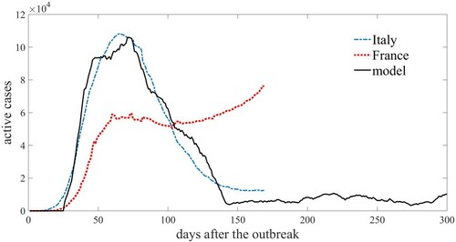
In general, researcher are still learning more about COVID-19 reinfections. Some studies recently concluded that immune responses from past infection reduce the risk of catching the virus again for at least 5 months [14]. As a consequence, the refractory period was chosen as ${\tau }_R=200$ days, consistent with what is known in the literature until today.

The network is supposed adaptive, that is individuals can change their links in response to the epidemic spread, as $n_{\text{rew}}(t)=0.5\cdot I(t)$, starting after the first 100 time steps.

As can be seen from the figure, the model follows qualitatively very well the real data of the epidemic observed in Italy, where social distancing and intervention policies have the effect of reducing active cases. Instead, the corresponding French case seems to suggest that the containment policies are either not effective enough or the people have not applied them with enough care.

6. Conclusions

We considered a classical SIRS model of epidemic spreading that explicitly accounts for the important elements that characterize epidemic spread, the infection and immunity periods as well as the strength of infection. We studied both a random-mixing model and a model based on a small-world network, where an adaptive behaviour is introduced so that susceptible individuals can avoid the infection. In our model, infected individuals transmit infection stochastically according to a fixed transmission probability or to their contact structure in the network. Then, the system evolves deterministically over a cycle that lasts ${\tau }_0$ time steps. Infected individuals move to the refractory state after an infection time ${\tau }_I$ and refractory individuals return to the susceptible state after immunity time ${\tau }_R$.

The random-mixing approach includes the main features of the epidemic, that is: pathogen extinction, endemic infection, persistence of disease with sustained oscillations, and dynamic extinction of the epidemic. These happen in different regions of the parameter space. However, in real life people change their social behaviour, both independently and in response to pathogen spreading. We accounted for these dynamics within a small-world network model, where individuals (nodes) adapt according to the state of their contacts. A susceptible individual who has the tie with an infected one, reconnects to a randomly chosen member of the remaining population, or to a randomly chosen member of the susceptible compartment. In this case, suppression of the endemic state happens when the isolated infected population becomes susceptible. Numerical simulations show the effects of adaptive evolving network as an useful strategy to decrease and/or controlling epidemic spreading.

Competing interests

The authors declare that they have no competing interests.

Disclosure statement

No potential conflict of interest was reported by the author(s).

References

- R.M. Anderson, and R.M. May, Infectious Diseases of Humans: Dynamics and Control, Oxford University Press, Oxford, 1991. https://doi.org/https://doi.org/10.1017/S0950268800059896
- M. Boguñá, C. Castellano, and R. Pastor-Satorras, Nature of the epidemic threshold for the susceptible-infected-susceptible dynamics in networks. Phys. Rev. Lett 111 (2013), pp. 068701.
- CDC (Centers for Disease Control and Prevention) “Interim Guidance on Duration of Isolation and Precautions for Adults with COVID-19” As of 13 February 2021; dataset available at https://www.cdc.gov/coronavirus/2019-ncov/hcp/duration-isolation.html
- A. D’Innocenzo, F. Paladini, and L. Renna, A numerical investigation of discrete oscillating epidemic models. Physica A 364 (2006), pp. 497–512.
- P.M. Gade, and S. Sinha, Dynamic transitions in small world networks: approach to equilibrium limit. Phys. Rev. E 72 (2005), pp. 052903.
- M. Girvan, D.S. Callaway, M.E.J. Newman, and S.H. Strogatz, A simple model of epidemics with pathogen mutation. Phys. Rev. E 65 (2002), pp. 031915–1.
- T. Goss, C.J. DommarD’Lima, and B. Blasius, Epidemic dynamics on an adaptive network. Phys. Rev. Lett 96 (2006), pp. 208701.
- H.W. Hethcote, H.W. Stech, and P. van den Driessche, Periodicity and stability in epidemic models: a survey, in Differential Equations and Applications in Ecology, Epidemics and Populations Problems, S. Busenberg, K.L. Cooke, ed., Academic Press, New York, 1981. pp. 65–82.
- H.W. Hethcote, M.A. Zhien, and L. Shengbing, Effects of quarantine in six endemic models for infectious diseases. Math. Biosc 180 (2002), pp. 141–160.
- S. Jolad, W. Liu, B. Schmittmann, and R.K.P. Zia, Epidemic spreading on preferred degree adaptive networks. PLoS ONE 7(11) (2012), pp. e48686.
- M. Kamo, and A. Sasaki, The effect of cross-immunity and seasonal forcing in a multi-strain epidemic model. Physica D 165 (2002), pp. 228–241.
- M. Kuperman, and G. Abramson, Small world effect in an epidemiological model. Phys. Rev.Lett 86 (2001), pp. 2909–2912.
- S.A. Lauer, K.H. Grantz, Q. Bi, F.K. Jones, Q. Zheng, H.R. Meredith, A.S. Azman, N.G. Reich, and J. Lessler, The incubation period of coronavirus disease 2019 (COVID-19) from publicly reported confirmed cases: estimation and application. Ann. Intern. Med 172 (2020), pp. 577–582.
- H. Ledford “COVID reinfections are unusual — but could still help the virus to spread” 14 JANUARY 2021; dataset available at https://www.nature.com/articles/d41586-021-00071-6.
- J. Li, Z. Jin, and Y. Yuan, Effect of adaptive rewiring delay in an SIS network epidemic model. Math. Biosc. Eng 16 (2019), pp. 8092–8108.
- W.M. Liu, H.W. Hethcote, and S.A. Levin, Dynamical behavior of epidemiological models with nonlinear incidence rates. J. Math. Biol 25 (1987), pp. 359–380.
- A.L. Lloyd, and R.M. May, Spatial heterogeneity in epidemic models. J. Theor. Biol 179 (1996), pp. 1–11.
- S. Milgram, The small world problem. Psychol. Today 2 (1967), pp. 60– 651.
- V. Nagy, Mean-field theory of a recurrent epidemiological model. Phys. Rev. E 79 (2009), pp. 066105.
- F. Paladini, I. Renna, and L. Renna, A discrete SIRS model with kicked loss of immunity and infection probability. J. Phys.: Conf. Ser 285 (2011), pp. 012018.
- F. Paladini, I. Renna, and L. Renna, A kiked epidemic SIRS model. Int. J. Bifurcation Chaos 22(10) (2012), pp. 1250251. 1-11.
- R. Pastor-Satorras, and A. Vespignani, Epidemic spreading in scale-free networks. Phys. Rev. Lett 86 (2001), pp. 3200–3203.
- R. Pastor-Satorras, C. Castellano, P. Van Mieghem, and A. Vespignani, Epidemic processes in complex networks. Rev. Mod. Phys. 87(3) (2015), pp. 925–979.
- I. Renna, When will the covid-19 epidemic fade out? medRxiv Preprint (2020). https://doi.org/https://doi.org/10.1101/2020.03.27.200451.
- L.B. Shaw, and I.B. Schwarz, Fluctuating epidemics on adaptive networks. Phys. Rev. E 77 (2008), pp. 066101.
- M.J. Silk, D.J. Hodgson, C. Rozins, D.P. Croft, R.J. Delahay, M. Boots, and R.A. McDonald, Integrating social behaviour, demography and disease dynamics in network models: applications to disease management in declining wildlife populations. Phil Trans R Soc B 374(1781) (2019), pp. 20180211. https://doi.org/https://doi.org/10.1098/rstb.2018.0211.
- M. Taylor, T.J. Taylor, and I.Z. Kiss, Epidemic threshold and control in a dynamic network. Phys. Rev. E 85 (2012), pp. 016103.
- I. Tunc, and L.B. Shaw, Effects of community structure on epidemic spread in an adaptive network. Phys. Rev. E 90 (2014), pp. 022801.
- D.J. Watts, and S.H. Strogatz, Collective dynamics of ‘small-world’ networks. Nature 393(6684) (1998), pp. 440–442.
- WORLDOMETERS (2020) https://www.worldometers.info/coronavirus/#countries (accessed 1 August 2020).
- G. Yan, Z.-Q. Fu, J. Ren, and W. Yang, Collective synchronization induced by epidemic dynamics on complex networks with communities. Phys. Rev. E 75 (2007), pp. 016108.
- D.H. Zanette, and S. Risau-Gusmán, Infection spreading in a population with evolving contacts. J. Biol. Phys 34 (2008), pp. 135–148.
- H. Zhao, and Z. Gao, Modular effects on epidemic dynamics in small-world networks. Europhys. Lett. 79(3) (2007), pp. 38002.